Detecting Road Intersections from GPS Traces Using Longest Common Subsequence Algorithm

Abstract

Intersections are important components of road networks, which are critical to both route planning and path optimization. Most existing methods define the intersections as locations where the road users change their moving directions and identify the intersections from GPS traces through analyzing the road users’ turning behaviors. However, these methods suffer from finding an appropriate threshold for the moving direction change, leading to true intersections being undetected or spurious intersections being falsely detected. In this paper, the intersections are defined as locations that connect three or more road segments in different directions. We propose to detect the intersections under this definition by finding the common sub-tracks of the GPS traces. We first detect the Longest Common Subsequences (LCSS) between each pair of GPS traces using the dynamic programming approach. Second, we partition the longest nonconsecutive subsequences into consecutive sub-tracks. The starting and ending points of the common sub-tracks are collected as connecting points. At last, intersections are detected from the connecting points through Kernel Density Estimation (KDE). Experimental results show that our proposed method outperforms the turning point-based methods in terms of the F-score.

1. Introduction

A road network is a system of interconnecting lines that represent the interconnecting roads in a given area [1,2,3]. Traditionally, the road networks are constructed from geographic surveying through devices, such as telescopes and sextants. These mapping devices are very expensive, and doing such surveys requires a huge amount of time and effort. As a result, such maps cannot be updated frequently [4]. With the development of Global Positioning System (GPS) technology in the last few decades, mobile mapping campaigns with GPS devices have replaced the surveying devices in urban areas and reduced the labor cost for the road map generation. Although, it is still time consuming for the campaigns to cover all streets on the map; thus, the map updates lag behind road construction substantially. Thanks to the ubiquitous use of hand-held GPS units, now we can easily obtain massive GPS trace data from a variety of road users, such as vehicle drivers, cyclists and pedestrians. This has simulated the development of automatic road network inference [5,6,7,8,9,10,11,12].

Road intersections play an important role in road networks. They can provide very useful information, such as connectivity, topology and allowable moving direction, which are not only beneficial to build the topology of the road network, but also helpful to generate the geometric representation of the road segments in the network. Based on the generated road network, we can further analyze the preferences of the travelers on route selection [13], the transition between different transportation modes [14], traffic density on the roads [15,16,17], the delays due to traffic jams [9,14,18,19], etc.

In the literature, some indirect methods have been proposed to detect the intersections by examining the moving direction changes of the road users on their trajectories. Karagiorgou and Pfoser detected turn samples from GPS traces by thresholding the moving speed and moving direction change [10]. The vector from the current point to its next adjacent point was used to describe the moving direction at this point. An agglomerative hierarchical clustering method was applied to cluster the turn samples into intersection nodes Wu et al. first found turning points from coarse-gained GPS traces by thresholding the moving direction changes [20]. To improve the concentration of the turning points, they collected the intersecting points, where the turning points converged. The X-means algorithm was applied in their work to cluster the converging points to intersections [21]. Wang et al. first detected the conflict points, where two or more traces cross, diverge or converge, through thresholding the road users’ moving direction change [22]. They then computed the spatial position and boundary circle of each road intersection from the conflict points. In our earlier work [23], we calculated the moving direction at each GPS point using the point ahead of it with a fixed distance to it, instead of the next point, and clustered the turning points with moving direction changes into intersection candidates. We finally checked the turn patterns to remove misdetected bends.

Although the researchers mentioned above have applied different techniques to detect the intersections, their algorithmic foundation is the same: an intersection is defined as a location or an area where the road users change their moving directions often. A limitation of these approaches is that it is difficult to determine an appropriate threshold for the moving direction change. A low threshold will lead to more spurious intersections being falsely detected, and a high threshold will result in more true intersections being undetected.

Different from the methods above, Fathi and Krumm designed a shape descriptor representing the distribution of GPS traces around a point and trained a classifier over the descriptor so as to distinguish intersection points from non-intersection points [24]. Their results showed that the detected intersections matched their ground-truth closely. However, they need to train a new shape descriptor for each new type of intersection, which is not suitable for automatic road map updating.

In this work, an intersection is defined by its own property as a location connecting three or more road segments in different directions. Based on this definition, a novel method is proposed to detect intersections from GPS traces based on the Longest Common Subsequence (LCSS) algorithm. First, pairwise GPS traces are aligned to find the longest common subsequences between them. The nonconsecutive subsequences are then partitioned into consecutive sub-tracks. Second, the starting and ending points of the common sub-tracks are collected as connecting points, if neither of the GPS traces start or end there. The density of the connecting points are estimated, and the local maximums on the density map are detected as intersections. At last, the pattern of the GPS traces converging or diverging at the connecting points around each intersection is checked to remove the false positive detections.

The initial results were written in a four-page paper and published in the 2016 IEEE International Geo-science and Remote Sensing Symposium [25]. In this paper, we elaborate our algorithm of intersection detection in more depth. Except the common sub-tracks in the same direction, we also find the common sub-tracks in the opposite directions by reversing one of the GPS traces and applying the LCSS algorithm to them. We improve the robustness of our algorithm against GPS errors, by checking patterns of the GPS traces meeting at the intersections and removing the intersections that are detected from one single GPS trace converging or diverging with all other traces. In addition, we evaluate the accuracy of the detected intersections thoroughly using the F-score measure, which considers both precision and recall.

The remainder of this paper is structured as follows. In the next section, we present the problem of intersection detection from GPS traces given the new intersection definition, followed by Section 3, which elaborates how to detect the common sub-tracks between pairwise traces and utilize the starting and ending points of these sub-tracks to identify intersections. Section 4 shows our experimental results. Lastly, the conclusion is drawn in Section 5.

2. Problem Statement

In this work, we define a road segment as a sequence of non-intersection geographical locations that connect two intersections. The road users often traverse a sequence of road segments, instead of a single road segment, to arrive at their destinations. On their journeys, they may traverse the same road segment and then split to different road segments; or they may traverse from different road segments to the same road segment. As a result, the generated GPS traces may converge from different road segments to the shared road segment or diverge from the shared road segment to different road segments. The converging and diverging points on the GPS traces are located at the intersections. Therefore, the intersections can be detected through finding the common sub-tracks of the GPS traces recorded on the same road segments. A common sub-track is a sequence of points that appears in the same relative order and occupies consecutive positions in both GPS traces. Each common sub-track corresponds to a shared road segment.

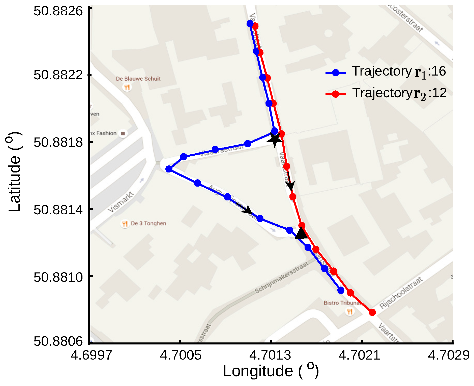
Figure 1 shows an example of two GPS traces diverging at one intersection and then converging at another intersection. The first GPS trace, which contains 16 points, is shown using blue lines with blue dots, indicating the point locations. There are 12 points in the second trace, shown in red lines with dots. The arrows show that the road users move from a higher latitude area to a lower latitude area in both traces. Both of the road users start their journeys on the same road segment, split to different road segments at the first intersection indicated using a black star, come together to another road segment at the second intersection indicated using a black triangle and end their journeys on this road segment. The generated GPS traces diverge at the first intersection and converge at the second intersection. We aim to find the common sub-tracks of the GPS traces, which correspond to the shared road segments both road users traverse, and identify the intersections from the starting and ending points of these sub-tracks.

3. Proposed Method

In this section, we first find the longest common subsequences between pairwise GPS traces, then segment them into common sub-tracks. The starting and ending points of the common sub-tracks, i.e., the converging and diverging points of the traces, are collected as connecting points. We then identify the intersections from the connecting points through KDE. Lastly, we examine the patterns of the GPS traces meeting at the intersections, so as to remove the false-positive intersections detected from one single trace converging or diverging with all other traces.

3.1. Longest Common Subsequence

A trace subsequence is a sequence of data points that appears in the same relative order within the original trace as a sub-track does, but does not necessarily occupy consecutive positions as a sub-track does. A common subsequence of two GPS traces is a subsequence present in both of them. A longest common subsequence is a common subsequence of maximal length. The most naive approach to find the longest subsequence would be to enumerate all subsequences common to both GPS traces and select the one of maximal length. However, it is very time consuming to apply this approach. To overcome this challenge, dynamic programming is employed to find the longest subsequence efficiently [26].

Dynamic programming is an algorithm for breaking a complex problem into a collection of simpler subproblems, solving each of those subproblems firstly and then using them to find the solution to the complex problem [27,28,29]. In our case, rather than finding the LCSS between two whole traces, we first find the LCSS between smaller prefixes of the traces and use them to find the LCSS between larger prefixes, until we find the LCSS between the whole traces.

We adopt the following notations. Suppose we have two GPS traces ${\mathbf{r}}^{\left(1\right)}$ and ${\mathbf{r}}^{\left(2\right)}$. Let ${\mathbf{r}}^{\left(1\right)}\left(t_1\right)$, $t_1=1,\dots ,T_1$ and ${\mathbf{r}}^{\left(2\right)}\left(t_2\right)$, $t_2=1,\dots ,T_2$ be points of ${\mathbf{r}}^{\left(1\right)}$ and ${\mathbf{r}}^{\left(2\right)}$, where $T_1$ and $T_2$ are the numbers of points in each trace, respectively. The first stage of implementing dynamic programming is to create a two-dimensional (2D) $T_1\times T_2$ length matrix L. The value at each cell, $L(t_1,t_2)$, represents the length of the longest common subsequences between the prefixes of the given traces, ${\mathbf{r}}^{\left(1\right)}\left(i\right)$, $i=1,\dots ,t_1$ and ${\mathbf{r}}^{\left(2\right)}\left(j\right)$, $j=1,\dots ,t_2$. It depends on the similarity of the points ${\mathbf{r}}^{\left(1\right)}\left(t_1\right)$ and ${\mathbf{r}}^{\left(2\right)}\left(t_2\right)$ and the values of its adjacent cells $\{L(t_1,t_2-1),L(t_1-1,t_2),L(t_1-1,t_2-1)\}$. We also create a 2D $T_1\times T_2$ arrow matrix B. The arrow at each cell, $B(t_1,t_2)$, indicates which of the adjacent cells $L(t_1,t_2)$ is calculated from, as shown Equation (2).

$$L(t_1,t_2)\stackrel{▵}{=}\{\begin{array}{ll}0,& \mathrm{if}{t}_1=0\mathrm{or}{t}_2=0\\ L(t_1-1,t_2-1)+1,& \mathrm{if}{t}_1,t_2>0\mathrm{and}d({\mathbf{r}}_1\left(t_1\right),{\mathbf{r}}_2\left(t_2\right))\le d_{thre}\\ max(L(t_1,t_2-1),L(t_1-1,t_2)),& \mathrm{if}{t}_1,t_2>0\mathrm{and}d({\mathbf{r}}_1\left(t_1\right),{\mathbf{r}}_2\left(t_2\right))>d_{thre}\end{array}$$

(1)

where $t_1\in [0,T_1]$ and $t_2\in [0,T_2]$. The geographical distance between two points, $d({\mathbf{r}}^{\left(1\right)}\left(t_1\right),{\mathbf{r}}^{\left(2\right)}\left(t_2\right))$, is used to measure their local dissimilarity. The distance threshold $d_{thre}$ should be chosen based on the road width and the expected GPS error.

$$B(t_1,t_2)\stackrel{▵}{=}\{\begin{array}{ll}\uparrow ,& \mathrm{if}L(t_1,t_2)=L(t_1-1,t_2)\mathrm{and}L(t_1-1,t_2)\le L(t_1,t_2-1)\\ \leftarrow ,& \mathrm{if}L(t_1,t_2)=L(t_1,t_2-1)\mathrm{and}L(t_1-1,t_2)<L(t_1,t_2-1)\\ \nwarrow ,& \mathrm{if}L(t_1,t_2)=L(t_1-1,t_2-1)+1,\end{array}$$

(2)

where $t_1\in [1,T_1]$ and $t_2\in [1,T_2]$.

Algorithm 1 FindPath.

Input: L, B

Output: ${\mathbf{g}}_1\left(k\right)$, ${\mathbf{g}}_2\left(k\right)$, $w_2\left(k\right)$, $w_2\left(k\right)$, $k=1\dots K$

Initialization $t_1\leftarrow T_1$, $t_2\leftarrow T_2$, $k\leftarrow 1$

2:  while $t_1+t_2>2$ do

if $t_1=1$ then

4:     $t_2\leftarrow t_2-1$

else if $t_2=1$ then

6:     $t_1\leftarrow t_1-1$

else

8:     switch $B(t_1,t_2)$ do

case $“\nwarrow ”$

10:        ${\mathbf{g}}_1\left(k\right)={\mathbf{r}}^{\left(1\right)}\left(t_1\right)$, ${\mathbf{g}}_2\left(k\right)={\mathbf{r}}^{\left(2\right)}\left(t_2\right)$

$w_1\left(k\right)=t_1$,$w_2\left(k\right)=t_2$

12:        $k\leftarrow k+1$

$t_1\leftarrow t_2-1$, $t_2\leftarrow t_2-1$

14:     case $“\uparrow ”$

$t_1\leftarrow t_1-1$

16:     case $“\leftarrow ”$

$t_2\leftarrow t_2-1$

18:    end if

20:  end while

if $L(1,1)=L(t_1,t_2)-1$ then

22:    ${\mathbf{g}}_1\left(k\right)={\mathbf{r}}^{\left(1\right)}\left(1\right)$, ${\mathbf{g}}_2\left(k\right)={\mathbf{r}}^{\left(2\right)}\left(1\right)$

$w_1\left(k\right)=1$,$w_2\left(k\right)=1$

24:  end if

${\mathbf{g}}_1\leftarrow \mathrm{reverse}\left({\mathbf{g}}_1\right)$, ${\mathbf{g}}_2\leftarrow \mathrm{reverse}\left({\mathbf{g}}_2\right)$

26:  $w_1\leftarrow \mathrm{reverse}\left(w_1\right)$, $w_2\leftarrow \mathrm{reverse}\left(w_2\right)$

Once the length matrix L and direction matrix B are built, the longest common subsequences are deduced by following the arrows backwards through matrix B. It starts from the last cell $(T_1,T_2)$ and ends at the first cell $(1,1)$. If the length decreases, the traces must have had similar data points. These two data points are added to the longest subsequences, ${\mathbf{g}}_1$ and ${\mathbf{g}}_2$, for each trace, respectively, and their time indexes in the original traces are added to $w_1$ and $w_2$, i.e., ${\mathbf{g}}_1\left(k\right)={\mathbf{r}}^{\left(1\right)}\left(w_1\left(k\right)\right)$ and ${\mathbf{g}}_2\left(k\right)={\mathbf{r}}^{\left(2\right)}\left(w_2\left(k\right)\right)$. Algorithm 1 elaborates the procedure.

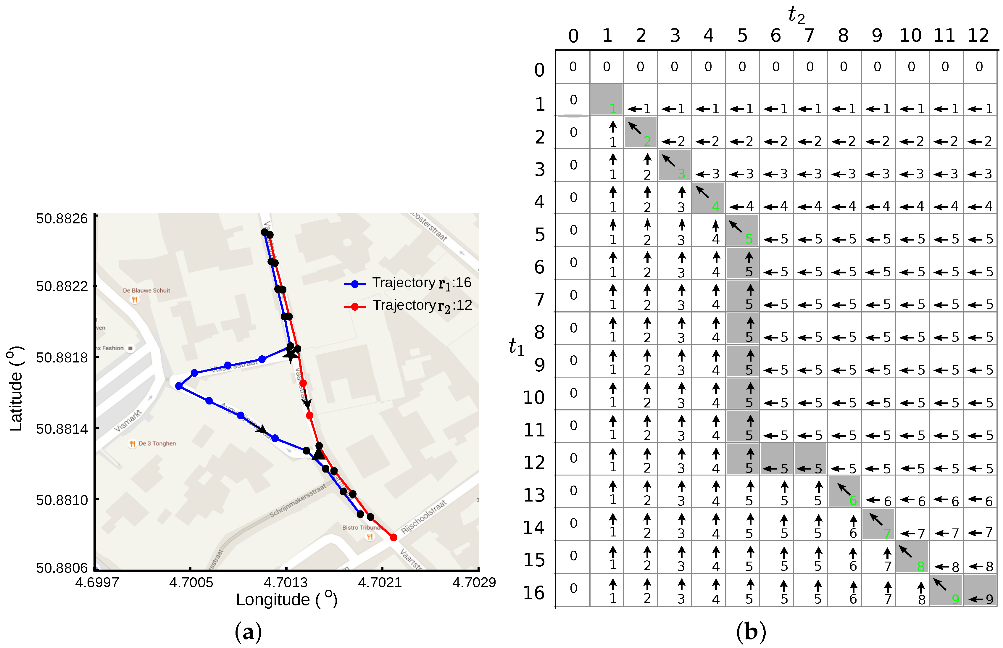
Figure 2 illustrates the procedure of finding the LCSSs between two GPS traces. Figure 2a shows the LCSS for each GPS trace using blue lines with black dots and red lines with black dots, respectively. In total, there are nine points in the LCSS for each trace. The LCSS for the first trace is expressed as ${\mathbf{r}}^{\left(1\right)}\left(t_1\right)$, $t_1=1,2,3,4,5,13,14,15,16$, and ${\mathbf{r}}^{\left(2\right)}\left(t_2\right)$, $t_2=1,2,3,4,5,9,10,11,12$ is for the second one.

Figure 2b shows the length matrix L and arrow matrix B in grids. The “backtrack” procedure starts at cell $(16,12)$ and follows the direction of the arrows to the first cell at $(1,1)$. The path through the matrix is indicated using cells with a gray background. Only the corresponding points to the cells with decreasing length are saved for the LCSS. The lengths of these cells are shown in green numbers.

3.2. Connecting Point Collection

A subsequence is a sequence of points that appear in the same relative order and do not have to occupy consecutive positions in the original trace. The longest common subsequence may correspond to more than one road segment. However, we are more interested in the common sub-tracks to both GPS traces, whose points do occupy consecutive positions in the original traces. Each common sub-track corresponds to one road segment that the road users traverse in both traces. Therefore, the starting and ending points of the sub-track correspond to the two ends of the road segment, i.e., intersections. The common sub-tracks between two GPS traces can be obtained by partitioning the longest common subsequences.

We first check the consecutiveness of the points of the longest common subsequences. Given the k-th points of the LCSSs for both traces, ${\mathbf{g}}_1\left(k\right)$ and ${\mathbf{g}}_2\left(k\right)$, and their time indexes in the original traces $w_1\left(k\right)$ and $w_2\left(k\right)$, they are nonconsecutive points if the next points ${\mathbf{g}}_1(k+1)$ and ${\mathbf{g}}_2(k+1)$ occupy positions far ahead of them in the original traces, i.e., $w_1(k+1)-w_1\left(k\right)>\xi$ and $w_2(k+1)-w_2\left(k\right)>\xi$, where ξ is a predefined threshold. In this work, we set ξ larger than one to avoid the deviating points on the trace, which are caused by GPS errors, being falsely detected as nonconsecutive points.

The longest common subsequence is segmented by these nonconsecutive points into common sub-tracks. If all points of the LCSSs are consecutive, we directly take the starting and ending points of the LCSSs as connecting points if they are not the starting and ending points of these two GPS traces.

As shown in Figure 2, the fifth points of the LCSSs are not consecutive in the original traces. For trace ${\mathbf{r}}^{\left(1\right)}$, the sixth point of its LCSS occupies the thirteenth position in ${\mathbf{r}}^{\left(1\right)}$. The fifth and sixth points of the LCSS are separated by seven blue dots. For trace ${\mathbf{r}}^{\left(2\right)}$, the sixth point of its LCSS occupies the eighth position in ${\mathbf{r}}^{\left(2\right)}$. The fifth and sixth points of the LCSS are separated by two red dots. Therefore, each LCSS is partitioned into two sub-tracks by the fifth point: the first sub-track containing five points and the second one containing four points. For the first trace, the detected common sub-tracks are ${\mathbf{r}}^{\left(1\right)}\left(t_1\right)$, $t_1=1,2,3,4,5$ and ${\mathbf{r}}^{\left(1\right)}\left(t_1\right)$, $t_1=13,14,15,16$. The common sub-tracks for the second trace are ${\mathbf{r}}^{\left(2\right)}\left(t_2\right)$, $t_2=1,2,3,4,5$ and ${\mathbf{r}}^{\left(2\right)}\left(t_2\right)$, $t_2=8,9,10,11$. The ending points of the first common sub-track for each trace, ${\mathbf{r}}^{\left(1\right)}\left(5\right)$ and ${\mathbf{r}}^{\left(2\right)}\left(5\right)$, are connecting points, and the starting points of the second sub-track for each trace, ${\mathbf{r}}^{\left(1\right)}\left(13\right)$ and ${\mathbf{r}}^{\left(2\right)}\left(8\right)$, are also connecting points. The starting points of the first common sub-track for each trace, ${\mathbf{r}}^{\left(1\right)}\left(1\right)$ and ${\mathbf{r}}^{\left(2\right)}\left(1\right)$, are not connecting points because they are also the starting points of the GPS traces. The ending points of the second sub-track for each trace, ${\mathbf{r}}^{\left(1\right)}\left(16\right)$ and ${\mathbf{r}}^{\left(2\right)}\left(11\right)$, are not connecting points because ${\mathbf{r}}^{\left(1\right)}\left(16\right)$ is the ending point of trace ${\mathbf{r}}^{\left(1\right)}$.

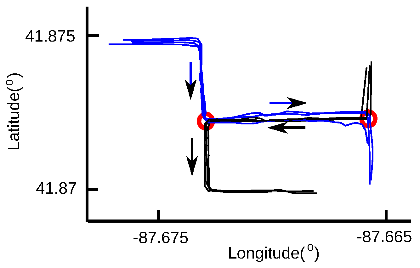
The procedure of detecting the LCSSs processes two GPS traces directionally, which start from the beginning of both traces and end at the ending of both traces. Therefore, only the common sub-tracks in the same direction can be detected. If the road users traverse the same road segment, producing two traces, but in the opposite directions, no common sub-tracks will be found between them. As shown in Figure 3, all of the GPS traces share the same road segment between two intersections, which are indicated by red circles. On this road segment, the road users travel from left to right in the blue traces, but from right to left in the black traces. No common sub-tracks will be found between the blue and black traces, although they do share the same road segment. Therefore, the connecting points at the ends of the common sub-tracks in the opposite directions will not be detected, leading to intersection detection being inaccurate. This can be solved by reversing the data points of the black traces.

Given a dataset of N GPS traces, we first find the common sub-tracks between each pair of GPS traces as elaborated above and collect the starting and ending points of the common sub-tracks as connecting points, if they are not the starting and ending points of these two GPS traces. We then reverse one trace in the each pair of the GPS traces and repeat the procedure again to find more connecting points.

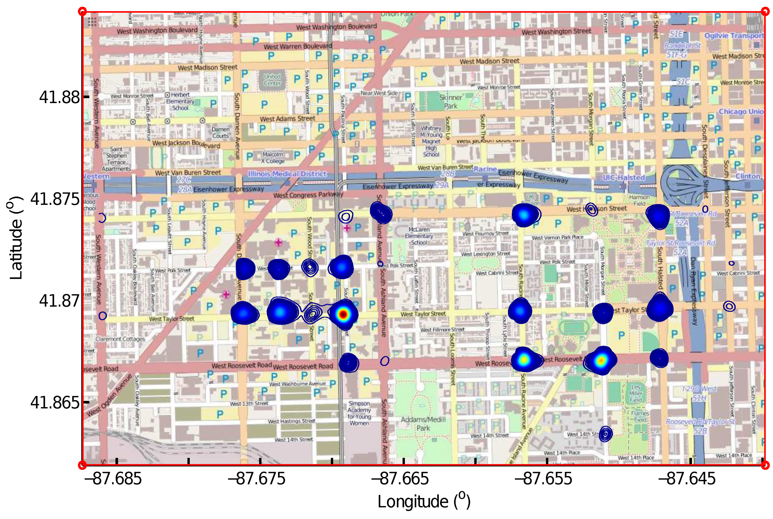
3.3. Intersection Extraction from Connecting Points

In this section, intersections are detected using the connecting points by estimating their density over the area covered by the GPS traces. We first discretize the geographical area into a two-dimensional (2D) grid of cells and count the number of the connecting points in each cell, producing a 2D histogram [5,30]. We then convolve this 2D histogram with a Gaussian smoothing function $N(0,{\sigma }^2)$, resulting in an approximation of the Kernel Density Estimation (KDE). The parameter σ exhibits a strong influence on the resulting estimate. A small σ can cause the 2D histogram to be undersmoothed, resulting in more than one intersection detected at the location of one true intersection. A big σ may lead to oversmoothing, then two adjacent intersections merge together on the density map. Therefore, the choice of σ should be made depending on the intersection size and the minimum distance between adjacent intersections.

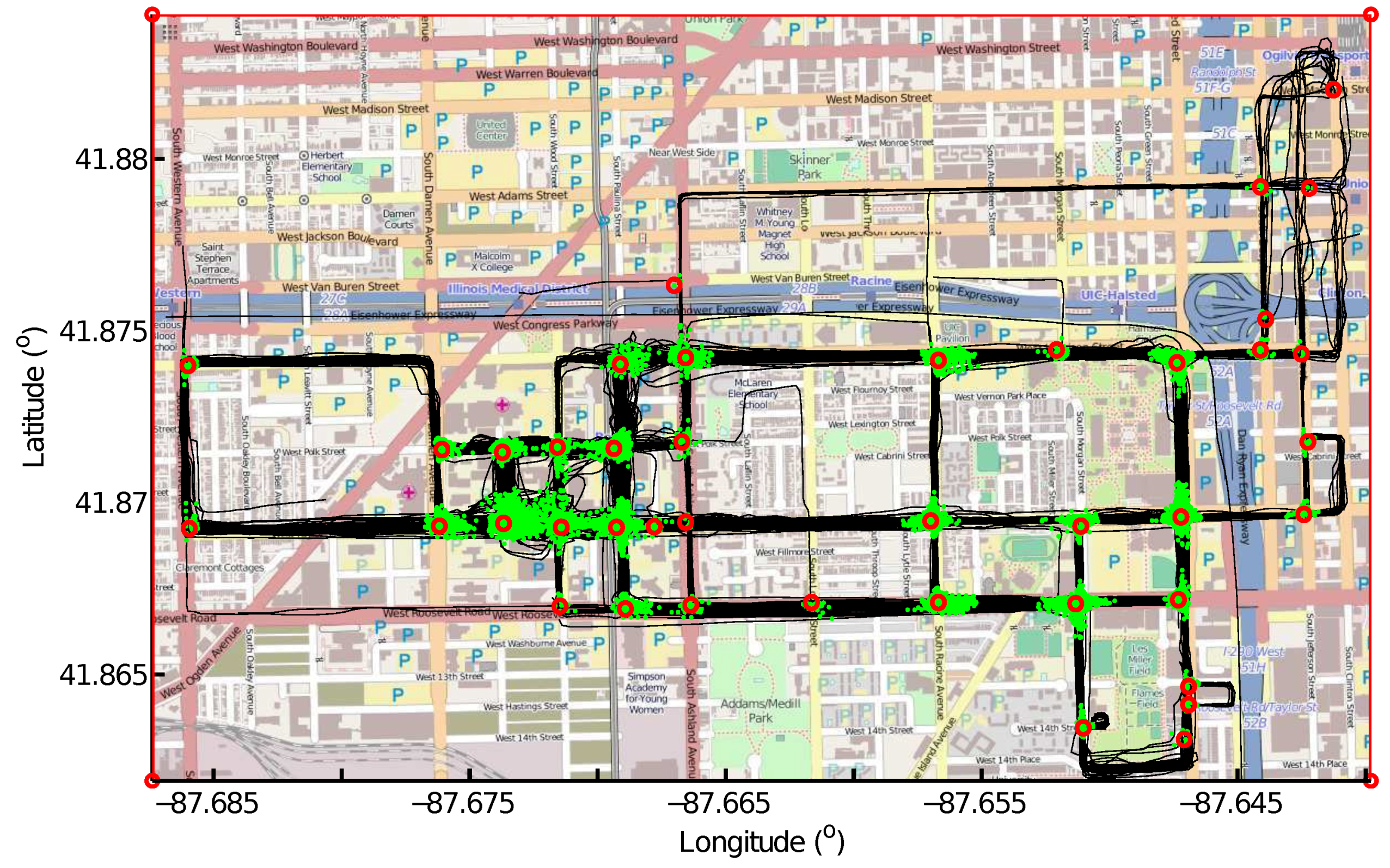
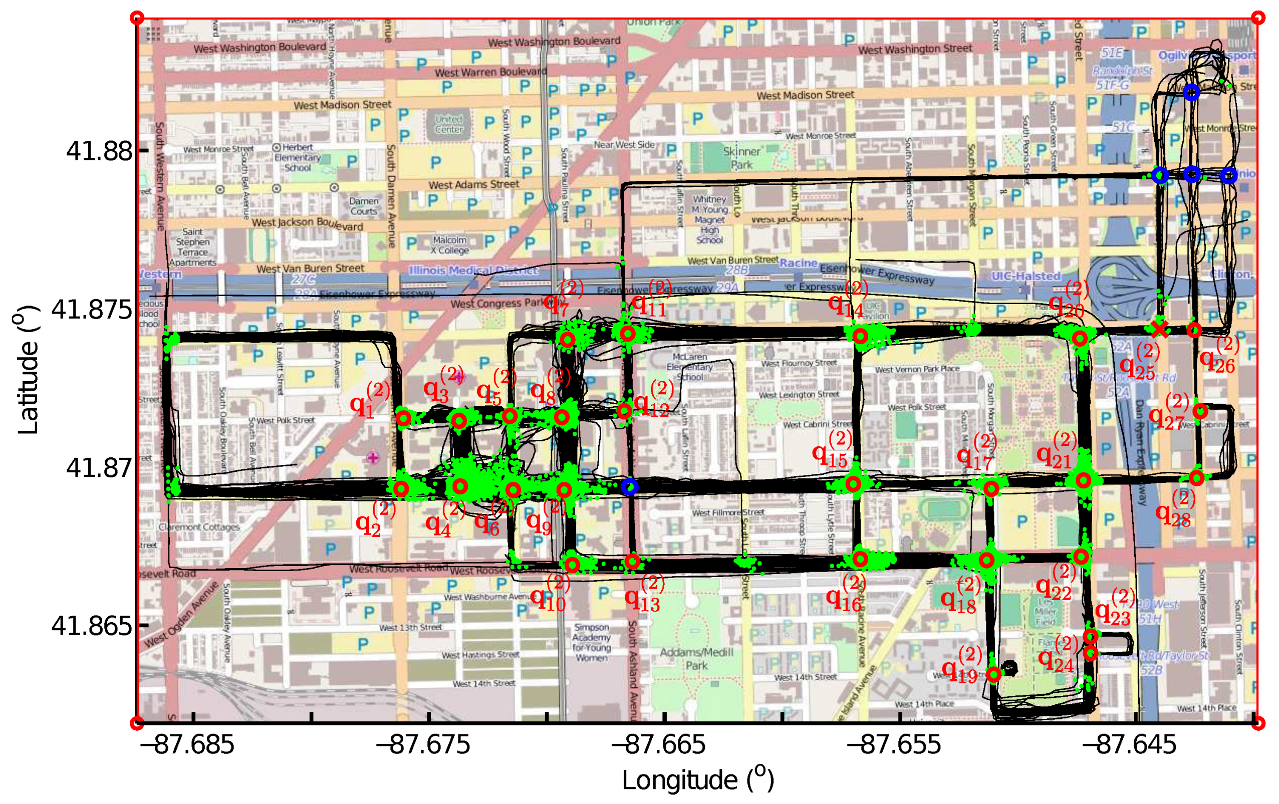
The local maximums on the density map, i.e., the cells that have greater values than their neighbors, are detected as intersections. The outputs of this step are the geographical locations of the detected intersections and the connecting points that belong to each intersection.

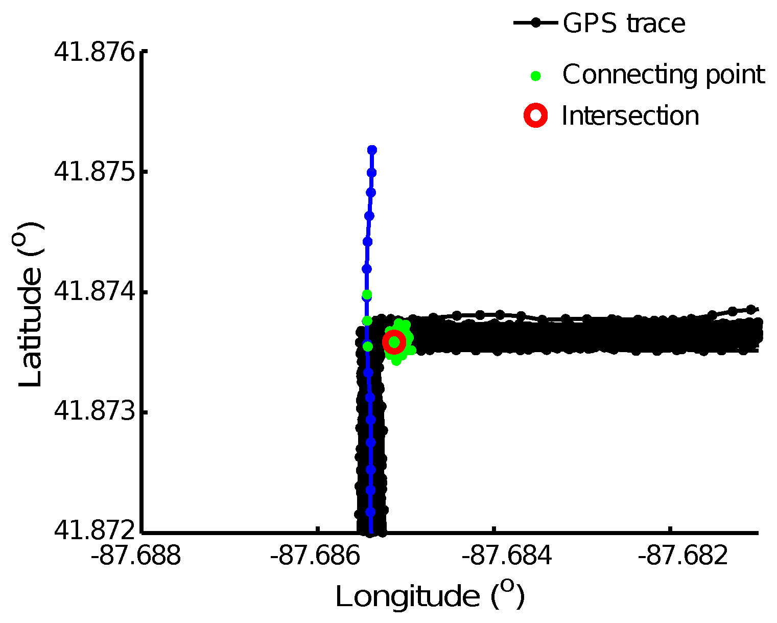
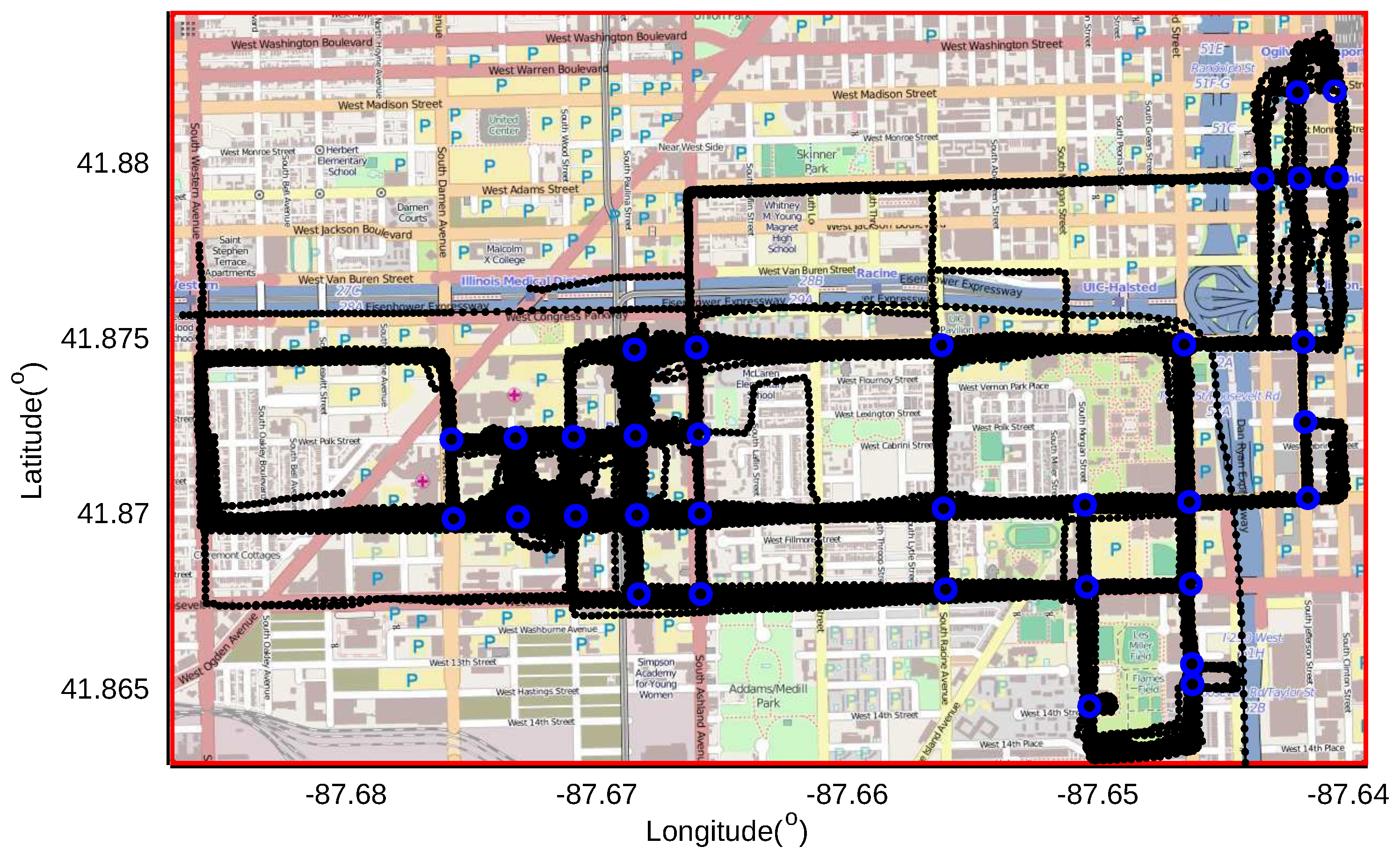
The connecting points are detected from GPS trace alignment using the LCSS algorithm. One single trace meeting with many other similar GPS traces at the same location can produce a large number of connecting points, resulting in a local maximum on the density map. However, this GPS trace can be an abnormal trace that deviates from the road because of GPS errors. An example is shown in Figure 4. This will lead to an intersection being falsely detected. Therefore, we need to check the patterns of the GPS traces meeting at one intersection and remove this kind of misdetected intersection, so as to make our algorithm more robust to GPS errors.

Given an intersection candidate $\mathbf{q}$, there are M connecting points belonging to this intersection ${\mathbf{r}}^{\left(i\right(m\left)\right)}\left(t_{i\left(m\right)}\right)$ and ${\mathbf{r}}^{\left(j\right(m\left)\right)}\left(t_{j\left(m\right)}\right)$, $i\left(m\right)\in [1,N]$, $j\left(m\right)\in [1,N]$, $t_{i\left(m\right)}\in [1,T_{i\left(m\right)}]$, $t_{j\left(m\right)}\in [1,T_{j\left(m\right)}]$, $m=1,\dots ,M$, where N is the number of the GPS traces in the dataset and $i\left(m\right)$ and $j\left(m\right)$ are the indexes of the traces producing the connecting points ${\mathbf{r}}^{\left(i\right(m\left)\right)}\left(t_{i\left(m\right)}\right)$ and ${\mathbf{r}}^{\left(j\right(m\left)\right)}\left(t_{j\left(m\right)}\right)$. Let $p_n$ be the number of connecting points that are detected by aligning trace ${\mathbf{r}}^{\left(n\right)}\left(t_n\right)$ with other traces using LCSS, $p_n={\sum }_{m=1}^{M}1\{i\left(m\right)=n\}+{\sum }_{m=1}^{M}1\{j\left(m\right)=n\}$. The connecting points are detected in pairs, one from ${\mathbf{r}}^{\left(n\right)}\left(t_n\right)$ and the other one from the other trace. Every connecting point is detected by aligning two traces; therefore ${\sum }_{n=1}^N{p}_n=2M$, where $p_n\le M$. If all connecting points are detected from aligning trace ${\mathbf{r}}^{\left(n\right)}\left(t_n\right)$ with every other trace, $p_n=M$. In this case, an intersection will be falsely detected from these connecting points if trace ${\mathbf{r}}^{\left(n\right)}\left(t_n\right)$ is an abnormal trace. For each GPS trace, we calculate $p_n$, $n=1,\dots ,N$, and remove this intersection candidate if any of $p_n$ equals M.

As shown in Figure 4, the intersection candidate shown in the red circle is removed from the true intersections because all of its connecting points shown in green dots are detected from aligning the GPS trace, indicated using blue lines with dots, with every of the other 152 GPS traces shown in black lines with dots. We admit that we will also remove true intersections connecting three road segments, in which the road users traverse two of the road segments very frequently, but through the third road segment only once. This detected intersection candidate will be removed until we have more GPS traces to confirm the existence of this third road segment.

3.4. Accuracy Measure

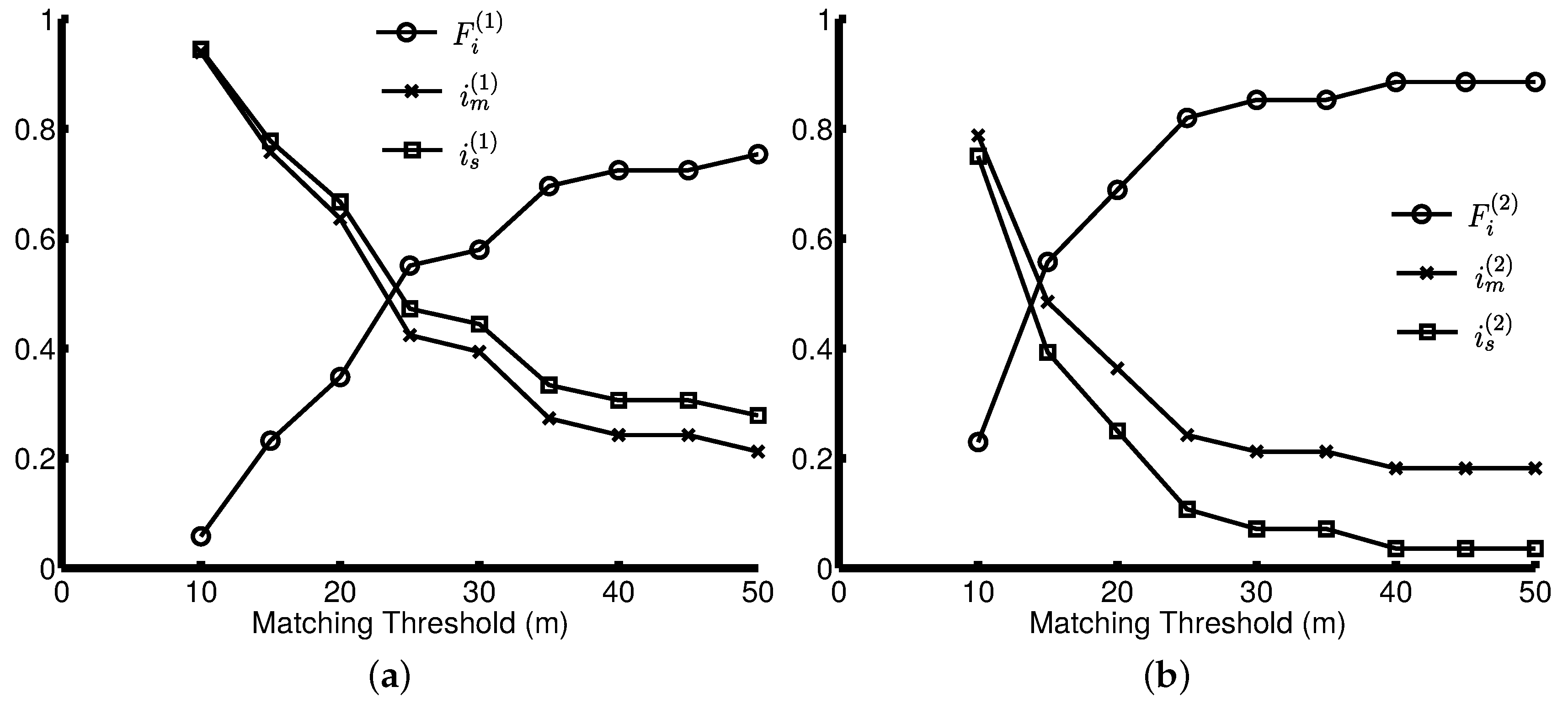
Because of the limited accuracy of the GPS traces, we may detect “spurious” intersections that are not matched to any intersection on the ground-truth map. Due to the low coverage of the GPS traces in some area, we may not detect all of the ground-truth intersections. An efficient intersection detection method is supposed to identify as many ground-truth intersections as possible and as few “spurious” and “missing” intersections as possible. Therefore, we measure recall, precision and the F-score of the intersection detection methods. The recall represents the proportion of the “matched” intersections among the “matched” intersections and the “missing” intersections, i.e., $\mathrm{recall}=I_c/(I_m+I_c)$, where $I_m$ and $I_c$ are the number of “missing” intersections and the number of “matched” intersections, respectively. The precision specifies the proportion of the “matched” intersections among all detected intersections, i.e., $\mathrm{precision}=I_c/(I_s+I_c)$, where $I_s$ is the number of “spurious” intersections. We use the well-known F-score [31,32], calculated using both precision and recall, as an overall accuracy measure:

$$\mathrm{F}-\mathrm{score}=\frac{2\times \mathrm{recall}\times \mathrm{precision}}{\mathrm{recall}+\mathrm{precision}}$$

(3)

4. Experimental Results

To evaluate the performance of our proposed method, we have applied it on a dataset of 889 GPS traces from the University of Illinois campus shuttles [33]. This dataset consists of 889 GPS traces and covers an area of $7\times 4.5$ km${}^2$. The traces are recorded at a sampling rate of 1 s to 29 s (average: 3.61 s). Figure 5 shows the GPS traces using black lines with dots indicating the point locations. OpenStreetMap is used as the ground-truth to measure the accuracy of the detected intersections. On the streets that were traversed by the shuttles, there are 33 ground-truth intersections, as indicated using blue circles in Figure 5.

4.1. Results of the Proposed Method

Because of GPS errors, some points deviate from the main trace. These points will break the common sub-sequences into more sub-tracks with a small $d_{thre}$ in Equation (1), leading to false connecting points detected on the road. With a big $d_{thre}$, the connecting points for adjacent intersections may be overlapped, resulting in these adjacent intersections being indistinguishable. Considering the maximum road width of 20 m and the GPS errors, we chose $d_{thre}$ as 40 m for this dataset.

Figure 6 shows the connecting points in green dots. Most of the connecting points are gathered at the intersections. At the top-right corner of the map, only a few connecting points are detected because of insufficient coverage from the shuttle. Some of connecting points are found on the road segments instead of at the intersections because of GPS errors. An example is shown in the red rectangle. One GPS trace deviates from the main road. Common sub-tracks between this GPS trace and other traces start in the middle of the road segment, rather than at one end of the road segment, resulting in false positive connecting points.

Figure 7 shows the kernel density estimation of the connecting points. The map is discretized into $1\times 1$ square meters cells. A 2D histogram is produced from the connecting points, and convolved with a normal distribution function $N(0,{\sigma }^2)$. We chose $\sigma =15$ meters depending on the size of the intersections and the minimum distance between two adjacent intersections. The density estimate shows clear peaks at the intersections on the map.

Figure 8 shows 41 intersection candidates in red circles, which are local maximums on the density map. Figure 9 shows the true intersections after checking the patterns of traces meeting at the intersection candidates. If all of the connecting points around one intersection candidate are obtained by one GPS trace intersecting with a number of other traces, it is removed because the existence of a road segment should be confirmed by more traces. In total, 13 candidates are removed, and 28 intersections are kept, including 27 true intersections shown in red circles and one spurious intersection ${\mathbf{q}}_{25}^{\left(2\right)}$ shown in a red cross. ${\mathbf{q}}_{25}^{\left(2\right)}$ is not matched to any intersection on the ground-truth map. The blue circles indicate the intersections we failed to detect.

Although no intersection is found at the location of ${\mathbf{q}}_{25}^{\left(2\right)}$ on the ground-truth map, the shuttles do pass by this location from three road segments in different directions. Because OpenStreetMap was downloaded as ground-truth map in August 2014, but this dataset was recorded in April 2011, the missing intersection ${\mathbf{q}}_{25}^{\left(2\right)}$ on the ground truth map could be caused by temporary traffic control or road construction. To confirm this, we checked the Google street view of this location on dates closest to the access dates and found that the road segment between the intersection ${\mathbf{q}}_{20}^{\left(2\right)}$ and ${\mathbf{q}}_{25}^{\left(2\right)}$ was under construction and impassable in October 2014. Therefore, there is a bend connecting two road segments existing at the location of ${\mathbf{q}}_{25}^{\left(2\right)}$ on the ground truth map, but an intersection of three road segments interconnecting is detected using our method.

4.2. Comparisons

In this section, we compare our proposed method with the turning point-based method in our earlier work directly [23]. Figure 10 shows the turning points in green dots and the intersections detected from turning points in red markers. The bends, which connect two road segments only, are removed through checking the shuttles’ turning patterns at these locations. In total, 36 intersections are detected after the bend removal, including 29 true intersections shown in red circles and seven spurious intersections shown in red crosses. Five of the ground-truth intersections, which are indicated using blue circles, are undetected using the turning point-based method.

Figure 11a,b shows the accuracy of the intersections detected from two different methods separately: Figure 11a is for the turning point-based method and Figure 11b for the proposed method. The matching threshold is defined as the allowable distance between the detected intersections and their positions on the ground-truth map. An intersection is considered as spurious if there is no ground-truth intersection within the allowable distance. With the lowest matching threshold of five meters, there are no true intersections on the ground-truth map matched to the intersections detected using the turning point-based method, neither using the proposed method. More intersections are correctly detected, as the matching threshold gets bigger. Therefore, the proportion of missing intersections gets lower, and the proportion of spurious intersections drops, as well, resulting in higher F-scores $F_i^{\left(1\right)}$ and $F_i^{\left(2\right)}$.

The turning point-based method detects more spurious intersections than our proposed method, resulting in higher $i_s^{\left(1\right)}$, but lower $F_i^{\left(1\right)}$ in Figure 11a, compared to $i_s^{\left(2\right)}$ and $F_i^{\left(2\right)}$ in Figure 11b. Figure 11a shows that the turning point-based method reaches an F-score of around $0.8$ with a matching threshold of 40 m. However, the F-score value of our proposed method reaches $0.85$ with a threshold of 30 m. It demonstrates that our proposed method has higher detection accuracy compared to the methods based on moving direction change. The average distance between the detected intersections and their ground-truth positions is $14.90$ m for our proposed method and $22.69$ m for the turning point-based method. This also confirms that the proposed method outperforms the other method.

5. Conclusions

We have presented a novel approach to identify intersections from GPS traces by detecting the common sub-tracks between pairwise traces using LCSS. The starting and ending points of these consecutive sub-tracks are collected as connecting points and used to find the intersections through KDE. The patterns of the GPS traces meeting at the intersections are checked so as to remove the false positive detections. Experimental results show that our proposed method achieves higher accuracy than the turning point-based method. Especially, we successfully differentiate true intersections from bends.

A drawback of our proposed method is the computational cost. Given N GPS traces, $\frac{(N-1)N}{2}$ pairwise traces are processed to detect the common sub-tracks using our method, while N traces are processed separately to find the turning points using the turning point-based method. Therefore, our computational cost is more expensive. In the future, we will pre-process the GPS traces to reduce the computational cost. For instance, the pairwise GPS traces will not go to the LCSS procedure if there are no overlapping points found between them. Additionally, we will work on inferring the existence and coverage of intersections statistically using a probabilistic method, instead of the two-valued logic in our current method. We will also test our algorithm in road networks with non-orthogonal road segments.

References

1. Shi, W.; Shen, S.; Liu, Y. Automatic generation of road network map from massive GPS, vehicle trajectories. In Proceedings of the 12th International IEEE Conference on Intelligent Transportation Systems, St. Louis, MO, USA, 4–7 October 2009.
2. Ahmed, M.; Karagiorgou, S.; Pfoser, D.; Wenk, C. A comparison and evaluation of map construction algorithms using vehicle tracking data. GeoInformatica 2014, 19, 601–632. [Google Scholar] [CrossRef]
3. Agamennoni, G.; Nieto, J.I.; Nebot, E.M. Robust inference of principal road paths for intelligent transportation systems. IEEE Trans. Intell. Transp. Syst. 2011, 12, 298–308. [Google Scholar] [CrossRef]
4. Schroedl, S.; Wagstaff, K.; Rogers, S.; Langley, P.; Wilson, C. Mining GPS traces for map refinement. Data Min. Knowl. Discov. 2004, 9, 59–87. [Google Scholar] [CrossRef]
5. Biagioni, J.; Eriksson, J. Inferring road maps from global positioning system traces. Transp. Res. Rec. 2012, 2291, 61–71. [Google Scholar] [CrossRef]
6. Edelkamp, S.; Schrödl, S. Route planning and map inference with global positioning traces. In Computer Science in Perspective; Springer: Berlin/Heidelberg, Germany, 2003; pp. 128–151. [Google Scholar]
7. Cao, L.; Krumm, J. From GPS traces to a routable road map. In Proceedings of the 17th ACM SIGSPATIAL International Conference on Advances in Geographic Information Systems, Washington, DC, USA, 4–6 November 2009.
8. Worrall, S.; Nebot, E. Automated process for generating digitised maps through GPS data compression. In Proceedings of the Australasian Conference on Robotics and Automation, Brisbane, Australia, 10–12 December 2007.
9. Niehoefer, B.; Burda, R.; Wietfeld, C.; Bauer, F.; Lueert, O. GPS community map generation for enhanced routing methods based on trace-collection by mobile phones. In Proceedings of the 1st International Conference on Advances in Satellite and Space Communications, Colmar, France, 20–25 July 2009.
10. Karagiorgou, S.; Pfoser, D. On vehicle tracking data-based road network generation. In Proceedings of the 20th International Conference on Advances in Geographic Information Systems, Redondo Beach, CA, USA, 7–9 November 2012.
11. Davics, J.; Beresford, A.R.; Hopper, A. Scalable, distributed, real-time map generation. IEEE Pervasive Comput. 2006, 5, 47–54. [Google Scholar]
12. Xie, X.; Philips, W.; Veelaert, P.; Aghajan, H. Road network inference from GPS traces using DTW algorithm. In Proceedings of the 17th IEEE International Conference on Intelligent Transportation Systems, Qingdao, China, 8–11 October 2014.
13. Zheng, Y.; Zhang, L.; Xie, X.; Ma, W.Y. Mining interesting locations and travel sequences from GPS trajectories. In Proceedings of the 18th International Conference on World Wide Web, Madrid, Spain, 20–24 April 2009.
14. You, Q.; Krumm, J. Transit tomography using probabilistic time geography: Planning routes without a road map. J. Locat. Based Serv. 2014, 8, 211–228. [Google Scholar] [CrossRef]
15. Vlahogianni, E.I.; Karlaftis, M.G.; Golias, J.C. Optimized and meta-optimized neural networks for short-term traffic flow prediction: A genetic approach. Transp. Res. Part C 2005, 13, 211–234. [Google Scholar] [CrossRef]
16. Herrera, J.C.; Work, D.B.; Herring, R.; Ban, X.J.; Jacobson, Q.; Bayen, A.M. Evaluation of traffic data obtained via GPS-enabled mobile phones: The Mobile Century field experiment. Transp. Res. Part C 2010, 18, 568–583. [Google Scholar] [CrossRef]
17. Xie, X.; Wong, K.; Aghajan, H.; Philips, W. Analyzing cyclists’ behaviors and exploring the environments from cycling tracks. In Proceedings of the Cycling Data Challenge 2013 Workshop, Leuven, Belgium, 14 May 2013.
18. Syberfeldt, A.; Persson, L. Using heuristic search for initiating the genetic population in simulation-based optimization of vehicle routing problems. In Proceedings of the Industrial Simulation Conference 2009, Loughborough, UK, 1–3 June 2009.
19. Xie, X.; Wong, K.; Aghajan, H.; Philips, W. Smart route recommendations based on historical GPS trajectories and weather information. In Proceedings of the Mobile Ghent, 2013, Ghent, Belgium, 23–25 October 2013.
20. Wu, J.; Zhu, Y.; Ku, T.; Wang, L. Detecting road intersections from coarse-gained GPS traces based on clustering. J. Comput. 2013, 8, 2959–2965. [Google Scholar] [CrossRef]
21. Pelleg, D.; Moore, A.W. X-means: Extending K-means with efficient estimation of the number of clusters. In Proceedings of the Seventeenth International Conference on Machine Learning (ICML ’00), Stanford, CA, USA, 29 June–2 July 2000.
22. Wang, J.; Rui, X.; Song, X.; Tan, X.; Wang, C.; Raghavan, V. A novel approach for generating routable road maps from vehicle GPS traces. Int. J. Geogr. Inf. Sci. 2015, 29, 69–91. [Google Scholar] [CrossRef]
23. Xie, X.; Wong, K.; Aghajan, H.; Veelaert, P.; Philips, W. Inferring directed road networks from GPS traces by Track Alignment. Int. J. Geo-Inf. 2015, 4, 2446–2471. [Google Scholar] [CrossRef] [Green Version]
24. Fathi, A.; Krumm, J. Detecting road intersections from GPS traces. In Proceedings of the Geographic Information Science, Zurich, Switzerland, 14–17 September 2010.
25. Xie, X.; Liao, W.; Aghajan, H.; Veelaert, P.; Philips, W. A novel approach for inferring intersections from GPS traces. In Proceedings of the 2016 IEEE International Symposium on Geoscience and Remote Sensing, Beijing, China, 10–15 July 2016.
26. Hirschberg, D.S. Algorithms for the longest common subsequence problem. J. ACM 1977, 24, 664–675. [Google Scholar] [CrossRef]
27. Denardo, E.V. Dynamic Programming: Models and Applications; Courier Corporation: North Chelmsford, MA, USA, 2012. [Google Scholar]
28. Sniedovich, M. Dynamic Programming: Foundations and Principles; CRC Press: Boca Raton, FL, USA, 2010. [Google Scholar]
29. Keogh, E.J.; Pazzani, M.J. Derivative dynamic time warping. In Proceedings of the First SIAM International Conference on Data Mining (SDM’2001), Chicago, IL, USA, 5–7 April 2001.
30. Scott, D.W. Multivariate Density Estimation: Theory, Practice, and Visualization; John Wiley & Sons: Hoboken, NJ, USA, 2015. [Google Scholar]
31. Yang, Y. An evaluation of statistical approaches to text categorization. Inf. Retr. 1999, 1, 69–90. [Google Scholar] [CrossRef]
32. Liu, B. Web Data Mining; Springer: Berlin/Heidelberg, Germany, 2007. [Google Scholar]
33. Laboratory, B.N.S. Available online: http://bits.cs.uic.edu/ (accessed on 21 December 2016).
Figure 1. An example of two GPS traces sharing roads. Two GPS traces diverge from one common road segment to different road segments at the first intersection, which is indicated using a black star, and then converge to another common road segment at the second intersection indicated using a black triangle.
Ijgi 06 00001 g001
Figure 2. LCSS problem of two GPS traces. (a) The longest common subsequences between trace r 1 and r 2 using black markers. There are nine points in the longest common subsequence for each trace. (b) The “backtrack” procedure of finding the optimal warp path of these two traces by following the arrows. The longest common subsequences are indicated using cells with green numbers.
Ijgi 06 00001 g002
Figure 3. GPS traces in opposite directions. On the road segment between two intersections indicated by red circles, no common sub-tracks can be found between the blue and black traces, because the road users traverse from left to right in the blue traces, whereas from right to left in the black traces.
Ijgi 06 00001 g003
Figure 4. A false positive intersection. One intersection candidate in the red circle is detected from the connecting points in green dots. It is a false positive because all of the connecting points are produced from 152 traces interconnecting with one single trace.
Ijgi 06 00001 g004
Figure 5. Chicago GPS traces and the ground-truth intersections. Eight hundred eighty nine GPS traces over 118 h are shown in black lines with dots that indicate the positions of GPS recordings. Thirty three ground-truth intersections are indicated using blue circles.
Ijgi 06 00001 g005
Figure 6. Connecting points. The connecting points are shown in green dots.
Ijgi 06 00001 g006
Figure 7. KDE of the connecting points. Peaks of the KDE are located at the intersections.
Ijgi 06 00001 g007
Figure 8. Intersection candidates. The intersection candidates are extracted from the connecting points by finding local maximums on the density map. In total, 41 candidates are detected.
Ijgi 06 00001 g008
Figure 9. Intersections detected from connecting points. By checking the patterns of the traces meeting at the intersections, 13 intersection candidates are removed, resulting in 28 true intersections shown in red circles.
Ijgi 06 00001 g009
Figure 10. Intersections detected from turning points. Thirty six intersection are identified, including 29 true intersections in red circles and seven spurious intersections in red crosses. Five intersections on the ground-truth map are undetected, which are indicated using blue circles.
Ijgi 06 00001 g010
Figure 11. Intersections’ accuracy analysis. (a) The accuracy of the intersections detected from turning points; (b) the proposed method based on connecting point detection.
Ijgi 06 00001 g011