


Remote Sensing-Based Yield Estimation of Winter Wheat Using Vegetation and Soil Indices in Jalilabad, Azerbaijan

1
Department of Satellite Communication and Remote Sensing, Institute of Graduate School, Istanbul Technical University, Istanbul 34469, Turkey
2
Department of Geomatics Engineering, Faculty of Civil Engineering, Istanbul Technical University, Istanbul 34469, Turkey
*
Author to whom correspondence should be addressed.
ISPRS Int. J. Geo-Inf. 2023, 12(3), 124; https://doi.org/10.3390/ijgi12030124
Submission received: 18 January 2023
/
Revised: 7 March 2023
/
Accepted: 9 March 2023
/
Published: 13 March 2023
(This article belongs to the Special Issue Geomatics in Forestry and Agriculture: New Advances and Perspectives)
Abstract
:Concerns about the expanding human population’s adequate supply of food draw attention to the field of Food Security. Future-focused analysis and processing of agricultural data not only improve planning capabilities in this field but also enables the required precautions to be taken beforehand. However, given the breadth and number of these regions, field research would be an expensive and time-consuming endeavour. With the advent of remote sensing and optical sensors, it is now possible to acquire diverse data remotely, quickly, and inexpensively. This study investigated the limitations and capabilities of remote sensing data application in the field of planning Food Security. As a result, Sentinel 2 and Shuttle Radar Topography Mission (SRTM) data were used to estimate winter wheat yields with a high degree of accuracy (98.03%) using the Mamatkulov technique and the MEDALUS model, which was both free and widely available. This method can make it possible to make predictions about the productivity of newly created crop fields or for which we do not have information about the productivity of previous years, without the need to wait for building regression models or any field studies. Considering the outcome, wide-range and larger analyses on this topic can be carried through.
1. Introduction
Satellite-based Remote Sensing (RS) data is now a fundamental aspect of cartography. RS satellites are used to collect these types of Earth Observation (EO) data from space. The growth of satellite technologies and RS systems has led to the creation of programmes that analyse RS data. These are known as RS and Geographic Information Systems (GIS). GIS is a technology that integrates hardware, software, and data to generate graphical representations of RS data and do spatial analysis.
Today, GIS is an essential and widely employed tool for the agricultural sector. These technologies specify new and improved analysis and evaluation methods, especially in agriculture. As the data have a geographic component, they can represent practically anything imaginable. Locally and globally, GIS applications play an essential role in agriculture. GIS has become a more valuable resource over the past decade as it has assisted farmers in improving production, reducing expenses, and providing an efficient tool for managing land resources [1].
Complex spatial analyses for agriculture can compare variables such as soil type, wind direction, rainfall, slope, aspect, terrain, or elevation to reduce flooding, drought, erosion, and disease risks to improve crop management, site suitability, and drainage planning. Using Unmanned Aerial Vehicle (UAV) data to identify areas of need and the underlying causes of food shortage, as well as land use and primary food crop statistics, GIS also contributes to global food security.
Providing the necessary food supply to support continuing population increase has become a growing challenge for today’s executive organisations. It is anticipated that agricultural production will have to double by 2050 to fulfil future food demands. GIS is utilised not just for real-time analysis but also for comparing previous data for those objectives above. Satellite visuals can be used to evaluate previous agricultural land use trends. This can assist in predicting and planning arable lands required to maintain future populations [2].
Planning for the food security of a region’s or even a country’s population places a significant emphasis on determining the efficiency of food production. As the foundation of many emerging economies, agriculture contributes significantly to the Gross Domestic Product (GDP). Therefore, the ability to acquire somewhat accurate yield estimations prior to harvest is crucial, so appropriate interventions can be implemented if poor yields are anticipated.
Winter wheat is one of the main staples in human consumption worldwide, as it has high nutritional value, multi-purpose usage, and affordability. Adding to its convenient, cost-efficient planting and irrigation, winter wheat has become one of the most important crops globally [3]. Therefore, yield estimation of winter wheat is an important topic for food security. In 2022, wheat accounted for 1 million 736.1 thousand tons (54.9 percent) of cereals and legumes produced in Azerbaijan. In addition, winter wheat also accounts for the largest share of total winter crop production at 62 percent [4]. As a result, advancement of the crop yield prediction is highly important for winter wheat, which can help organisations and individuals to manage and plan agriculture [5].
The estimation of productivity is crucial to economic progress [6]. These projections warn decision-makers about the possibility of crop yield losses and enable prompt importing and exporting decisions. As can be seen, yield estimation methods are a crucial component of these processes. Obtaining yield estimations with GIS is a crucial application for reducing costs and automating processes.
There are two standard traditional techniques for calculating crop yield: empirical-statistical and crop growth models [7]. These techniques are derived from field reporting.
The first is the classic method used in many regions, which is based on traditional data collection procedures for crops and yield estimation based on field reports from the ground [8].
Some empirical-statistical models consider long-term crop yields and factors that influence crop production in a certain region. The yield of the crop is then linked to the effective parameter using an empirical equation, and the coefficient of each factor is determined [9]. Nowadays, the crop yield is estimated using these coefficients. Each collection of empirical models ties several parameters to crop yield. Models of crop growth anticipate crop production as a function of the complicated interaction between many physiological processes and the environment. These models predict the potential for biomass output using a daily crop growth simulator. There are significant operational challenges associated with these approaches, including the need for too many ground factors, proper data gathering, and expensive costs.
RS techniques concurrently eliminate the drawbacks of conventional procedures [10]. 1970 marked the beginning of crop yield estimation techniques based on satellite imagery and the use of satellite imagery in agriculture for EO. Previously, these technologies were not commonly used since satellite photos were costly and lacked spatial resolution. By eliminating the mentioned disadvantages, high spatial and spectral resolution images have been produced since 1990, and many studies have employed these techniques.
Analysis of RS data alone or in conjunction with other ancillary data (such as soil moisture) permits the estimation of crop productivity prior to harvest [11]. The capability of RS to offer information on crop status and health is a significant factor in estimating potential crop production.
In a recent study conducted in China for the crop growth model of the simple algorithm for yield estimate (SAFY) of wheat, researchers incorporated the leaf area collected from Sentinel-2 remote sensing data. Several SAFY parameters, including the Emergence Date (D0), the Effective Light energy utilization rate (ELUE), etc. are fine-tuned using the Shuffled Complex Evolution Optimization with Principal Component Analysis (SP-UCI) optimization method. This crop growth model was developed using multiple data including RS of a certain time period [12].
Crop yield growth models are usually developed using machine learning technologies and require a significant time period for a machine to observe the trends and reports [13]. These RS data-based analyses make the applicability of many methods possible. For instance, in a previous study conducted in Türkiye, the relationship between soil quality data such as productivity and salinity was proven by employing GIS and RS technologies [14]. The findings demonstrated that rising Electrical Conductivity (EC) values resulted in lower cotton and wheat yields. Crop yields decreased linearly when salinity rose beyond the threshold for cotton and wheat. According to the research, RS and GIS techniques are practical approaches for predicting agricultural productivity.
In a study carried out by Arab and Tokhi in 2020, Landsat 8 earth imagery visuals from 2017, 2018, and 2019 were used in order to map the RS-based NDVI, LAI, and NDWI on grape yields to determine their correlation with grape yield estimation [15]. Different stages of growth were observed, and different methods were used to develop yield estimation models based on an automatic model using RS-based time-series imagery. The results indicated that of all the vegetation indices, NDVI had the highest correlation with yield prediction. According to the results obtained, we can conclude that vegetation indices, especially NDVI can be used for forecasting yields. Time series based on satellite imagery can achieve reliable results on yield prediction models.
A study conducted for determining suitable landmass for agricultural purposes in Egypt used the MEDALUS methodology for developing the Soil Quality Index (SQI) formula. The equation was changed to be adjustable so that it may take into account various soil characteristics that can have an impact on soil quality and hence alter the outcome of Soil Quality (SQ) [16].
Additionally, many research papers had determined that the result range of the SQI is changeable depending on the laboratory and RS-derived sub-parameters [17,18].
Another study addressed the topic by using multiple components such as vegetation, and Soil Quality and applied the MEDALUS method on which our study also took its basis: in research that was carried out for near real-time yield forecasting on cotton areas of Jarkurgan district, Uzbekistan, during the timeline from April through August 2019, used geospatial analyses of RS-based multi-temporal vegetation and multi-source SQ indices such as soil salinity, soil texture, slope gradient, soil depth, drainage condition, the content of total calcium carbonate in soil, and soil organic matter rate [19,20]. For this exact purpose, the MEDALUS method for indicating the SQI was used, which consisted of both RS and laboratory data. As a result, the correlation between those indices and crop yield had been confirmed with a 96% validity rate. Although the method suggested by the researchers was relatively simpler and more apprehensible to apply for yield forecasting purposes, it was not quite accessible due to the need for field information such as laboratory results for indicating SQI.
However, unlike the Mamatkulov approach, we estimated those indices only using RS data and GIS methods without applying any field information such as laboratory-derived SQI indicators. In this context, the main purpose of the study is to forecast the yield of the cropland which we lack information on the productivity of prior years, without the need for any field research or regression models.
Unlike the other RS-based empirical-statistical yield estimation methods which require multiple-year trends and RS data to develop regression models, in this method, only the combination of bare soil, sprouted field, and elevation frames are needed. In addition to that, contrary to the other RS-based Yield estimation methods, in this article possibility of estimating yield forecast without the need for the regression models based on the previous yield reports was tested. To conclude everything that has been stated so far, for this research, the applicability of the satellite-based data and calculations on indicating SQI elements and Yield forecasts were tested.
The study paper is organized as follows: Section 2 describes the study area and several experimental data such as Sentinel 2 mosaic datasets and SRTM Digital Elevation Model (DEM) data. Section 3 describes the methodology used in this study. Section 4 discusses the test results and discussion. Section 4 presents the major conclusions of the study.
2. Data Description
For this study, a 5.384 sq. kilometres test area belonging to the State Reserve Fund was selected in the village of Privolnoye, which is located within the 48.5′ E 39.2′ N provincial borders of Jalilabad, Republic of Azerbaijan as shown in Figure 1a,b,d. The low-mountainous semi-arid area is planted with durum winter wheat.
Durum wheat differs from soft wheat in signs, appearance, and other signs. The spikes of durum wheat are very thick and tough. The grains vary in different colours such as white, red, light, or dark amber. The bays are long as the spike, upright. The grains do not fall on the ground when they are ripe as they are tightly covered with external and internal flower scales. the number of chromosomes in the plant is 28. Because durum wheat flour has better quality than flour of soft wheat, it is used in pasta production more [21].
The atmospheric factors demanded for the first period of the development of winter wheat crops are different from spring wheat. Winter wheat has a longer vernalization period [21].
Winter wheat in Azerbaijan is mainly planted during the period of late September to early November and then harvested by the end of May or the beginning of June of the next year. Winter durum wheat usually is not irrigated in semi-arid high-productivity areas, thus, the water consumption balance model for yield estimation is applicable based on the soil moisture [21].
Vegetation analysis was applied to imagery, which was ingested during the springtime, April 2022, while soil quality indices such as Soil Texture Index (STI), Normalized Difference Moisture Index (NDMI), Total Inorganic Carbon Index (TICI), Soil Salinity Index (SI) were calculated based on the previous timeline, August 2021.
Time Series Analysis of the NDVI values during a year retrieved from GEE. Using the information mentioned in Figure 1c, bare soil and high vegetation periods were defined. Between the time periods of early August 2021 and late September 2021, the vegetation trends are following the lowest stable values.
Optic and radar data combinations such as Sentinel 2 and SRTM were applied. Two level-2 Sentinel 2 products covering bare soil before planting from 23 August 2021, and green fields of the tillering winter wheat from 15 April 2022, were obtained as shown in Figure 2.
30 m-resolution SRTM DEM data (N39E048) was obtained using the SRTM Downloader plugin in Quantum Geographic Information System (QGIS) as shown in Figure 3.
3. Methodology
3.1. Mamatkulov’s Approach to Yield Estimation
Agriculture monitoring based on RS and GIS is a vital component of the food safety information system, which provides accurate and timely crop area estimates and crop output projections on a national, regional, and global scale.
Multiple methodological approaches for measuring crop efficiency with RS data have been improved so far. Some of these procedures are straightforward, while others are more complicated.
There are numerous methods for estimating crop yields using satellite data and GIS. These techniques fall into three classes:
- RS techniques which are founded on empirical-statistical models.
- RS approaches which are based on an equilibrium model of water use.
- RS approaches that utilise biomass estimating models.
Mamatkulov’s approach is suitable for determining the yield’s main elements as indices, and unlike other methods, it does not need previous years’ yield results and data, which makes it relatively more time efficient [19].
In the Mamatkulov technique [19], which is based on Monteith and the biomass estimating model, the Yield Gradient Index (YGI) of the product is computed according to the level of the soil site as follows:
Here, A represents the vegetated area of the region, computed using the Normalized Difference Vegetation Index (NDVI), The range of B’s SQI is 0 to 100, and C is the crop coefficient for calculating efficiency which is estimated using evapotranspiration.
This study used geospatial analysis of multitemporal satellite data, groundwater conditions, soil salinity, and ground truth data to monitor crops in real-time and forecasted yields in low- and high-productive cottonfield areas of Jarkurgan district of Surkhandarya region, Uzbekistan.
False Color, NDVI, and SI analyses of areas were performed utilising multi-temporal Sentinel 2 data from April and August 2019 to track the phenology of cotton vegetation and predict its crop yield.
In our approach, the formula is therefore modified as follows:
where Kc is the special Kappa crop coefficient we are using as a crop coefficient based on the crop growth model.
In Mamatkulov’s approach, results are calculated by centners, and in 0 to 100 scale to determine YGI. However, in our study, we used tonnes. Therefore, the formula was also modified according to the desired measurement unit.
Indicators derived from spatial-temporal Sentinel 2 imagery, together with other auxiliary environmental data such as groundwater status, soil quality (SQ), and expert knowledge, can provide more accurate crop growth and production predictions.
3.1.1. Normalized Difference Vegetation Index
RS data is widely utilised for vegetation mapping and monitoring. Due to the structure of ‘green’ leaves, healthy vegetation exhibits the greatest reflection at near-infrared wavelengths and the greatest absorption at red wavelengths due to the presence of chlorophyll [22]. NDVI is generated from satellite data combinations and calculated using the formula below.
Here, NIR refers to light reflected in the near-infrared spectrum, and R refers to light reflected in the red region of the spectrum.
In general, NDVI values range from −1 to 1 [22]. Negative values indicate water bodies such as clouds, water, and snow, positive values close to 0 indicate rocks, bare land, buildings, and roads, and values greater than 0.2, depending on the region, indicate green areas. Large values (0.6 to 0.8) reflect temperate and tropical woods, whereas medium values (0.2 to 0.3) represent shrubs and meadows. Areas of empty rock, sand, or snow correspond to NDVI values of less than 0.1 [22].
3.1.2. Crop Coefficient
The Kappa coefficient for crops (Kc) is a specific coefficient for a particular plant crop. Typically, the Kc is calculated experimentally on fields. This value represents multiple changes in the effects of the soil, crop, climate conditions, and crop-management techniques. Every crop field has a set of specific crop coefficients based on the climate and the chlorophyll rates. This method is based on research on wheat fields in Egypt [23]. In that exact research, it had been determined that there is a correlation between the NDVI index and Kc.
According to the experimental data, usually is equal to 1.2, while is 0.1 [23].
The final approach that we are taking into consideration is the Kc calculation method based on Leaf Area Index (LAI). The research was applied to two vineyards located in Israel, using optical and SAR RS imagery [24]. As a result, the quadratic correlation between Kc and the LAI in that research was confirmed.
LAI—as one of the most significant biophysical variables used to track plant development and production, is an index that is defined as leaf area per unit of ground area. For large agricultural areas, determining LAI by field surveys is time-consuming and challenging. Since they can offer reliable, up-to-date, and consistent spatial and temporal coverage and resolution, as well as usability and ease of use, indirect approaches, such as the utilization of geographic data gathered by RS, have grown popular. Furthermore, LAI cannot be measured over a vast area. Because of this, it is thought that using satellite data to calculate LAI values quickly and precisely is the most appropriate approach [25].
3.1.3. Soil Quality Index
SQ is one of the most prevalent notions to have arisen in recent years, and it is used to analyse soil in many systems. In practice, soil quality is evaluated based on soil effects on crop yield, erosion, surface and ground, food, and air quality [26].
Maintaining good agricultural yields requires the evaluation of management-induced changes in SQ. Based on relative soil properties and crop output, a wide variety of cultivated soils must be properly identified using the SQI. Numerous attempts have been made to estimate SQI for vast soils around the world, but there is no defined standard approach. Therefore, there is an urgent need to produce a user-friendly and trustworthy SQI by comparing the various methodologies now available.
It can be utilised as a standard in the yield estimation calculations of the SQI result regardless of the product type. The SQI varies among soil types in the study and spans from 0 to 1. (1 is the maximum SQI). Using the Mamatkulov approach, these signs were later evaluated on a scale ranging from 0 to 100.
The relationship between crop yield and SQ is undeniable, yet SQ in different tiers may not be the same, influencing crop yield. However, a stronger correlation coefficient was discovered in the 0–20 cm soil layer than in the deeper soil profile, most likely due to the greater plant root density in the topsoil [27].
Traditionally, the MEDALUS approach is calculated using different SQ indices by rooting the multiplied indices by n-degree which n is the number of indices [28]. However, these calculations usually include indices obtained from laboratory results.
In the MEDALUS approach [28], in which we choose to calculate the SQI variable utilised in the formula using only RS data, we evaluate the SQ based on the physical, chemical, and biological soil qualities, RS data, and GIS methodology. In our approach, different SQ parameters were re-evaluated by being calculated via RS data.
Using DEM and Sentinel-2 data, physiographic units were identified in order to meet the research objective:
- field report data to verify the physiographic outputs.
- construction of the spatial model for the SQI evaluation
- estimating the Yield gradient index including validation percentage using the field capacity and observed values of the survey area.
SQ calculation we developed based on the MEDALUS method is based on the following formula [19].
Here, the SGI slope gradient index, SDI soil depth index, and NDMI is showing drainage status.
Soil Texture Index
Many physical and chemical properties and behaviours of soil, such as water storage, cation exchange capacity, soil fertility, internal drainage, and absorption capabilities, are believed to be influenced by soil texture [29,30].
It is much simpler to collect RS data for detailed descriptions of expansive regions. Therefore, RS data can serve as valuable supplementary variables for estimating surface soil texture. Using laboratory soil reflection data and satellite RS data [31], numerous researchers have focused on the GIS estimation of STI [32].
Soil Depth Index
Topsoil is the soil’s uppermost layer. It consists of mineral particles and biological stuff and often spans between 13 and 25 centimetres deep. Together, they provide a substrate capable of retaining water and air, so fostering biological activity.
As plants derive the majority of their important nutrients from the topsoil, it typically contains a high root density. It also harbours extensive bacterial, fungal, and insect activity, where SQ degrades and becomes less accessible to plants. A healthy topsoil layer is home to a diverse community of microorganisms. As a strong correlation was discovered in the 0–20 cm soil layer with the SQ than in the deeper soil profile, soil depth is essential for agriculture, more precisely, yield estimation methods [33]. According to current statistics, the average soil depth in agricultural areas should range between 20 and 30 centimetres [33].
Normalized Difference Moisture Index
The Normalized Difference Moisture Index (NDMI) has supplied information on forest health and is particularly effective for detecting damaged forests and forest recovery following epidemics (individual stages of degradation and recovery mode).
NDMI is determined as the ratio between the difference and the sum of the refracted radiations in the NIR and Shortwave infrared (SWIR) areas to determine the crop or soil water stress level.
The interpretation of NDMI’s absolute value enables the rapid identification of farm or field regions with water stress issues. NDMI is straightforward to interpret: its values range from −1 to 1, and each number corresponds to a distinct agricultural condition, irrespective of the crop. NDMI is computed with the following formula [35]:
Total Inorganic Carbon Index
Calcite is the most stable polymorph of calcium carbonate, a carbonate mineral (CaCO3). It is a prevalent inorganic mineral, particularly as a component of limestone. Calcite has a hardness of 3 based on scratch resistance on the Mohs scale of mineral hardness. Large calcite crystals are utilised in optical equipment, and calcite-rich limestone has several applications [36].
According to research for estimating inorganic carbon rate in water bodies [37], the Total Inorganic Carbon Index (TICI) is calculated using Coloration Index (CoI) on MODIS data:
This approach is alterable with the Sentinel-2 data. Thus, TICI becomes:
Salinity Index
In dry and semi-arid places where precipitation exceeds evaporation, salinization of the soil is one of the most prevalent land degradation processes. Under such climatic conditions, soil-soluble salts build and degrade soil characteristics, causing a loss in soil production. Soil salinization is the enrichment of soil with soluble salts that provide information on the soil’s response to the salt. Soil salinity in irrigated areas is becoming a severe problem for agriculture. Globally significant land areas have decreased in value and production due to the salinization of their soils [38]. Salinity is widespread in irrigated soils as a result of the accumulation of soluble salts from the continual use of irrigation waters containing high or moderate concentrations of dissolved salts [39].
The combination of RS and GIS is utilised to characterise various salt-affected soil data. The most used technique for calculating salinity index is the calculation of distinct index and ratio imagery utilising infrared and visible spectral bands. In general, dry soil has a higher reflectivity, and no red-zone absorption was considered in the construction of vegetation indices. Satellite photos and false colour combinations are visually interpreted to identify places damaged by salt. RS and GIS tools are used to examine digital RS data. The formula for the SI has been constructed for the Sentinel 2 products using Blue, Green and Red bands with ρ492.4, ρ559.8, and ρ664.6 wavelengths [19,38,39].
During the dry season, white or bluish-white salt crusts on the surface are excellent signals for the detection and correlation of saltiness. Satellite RS data provide real-time information regarding these soils, proving to be a powerful analytical tool for predicting salt-affected regions and crops affected by salinity.
Slope Gradient Index
DEM is a digital cartography dataset representing a continuous topographic elevation surface through a sequence of cells. Each cell indicates the Z height of a feature at certain X and Y locations. DEMs are a representation of the “bare earth” since they incorporate elevation data for geological ground features such as valleys, mountains, and landslides, to mention a few. They lack elevation information for non-ground elements such as flora and structures [40].
DEMs are typically derived using RS-collected radar data, although they can also be derived by field research. DEMs are the most popular base for digitally created relief maps and are frequently utilised in GIS.
Using DEM and GIS, this article intends to construct a method to derive and map the Slope Gradient (SG) index. “Slope” characterizes the change rate of DEM in every pixel. The spatial distributions of SG collected reveal regions with abnormally high SG levels [40].
Several algorithms exist to calculate SGI from DEM. QGIS uses a planar method for this reason. In this approach, the rate of change (delta) of the surface in the horizontal (dz/dx) and vertical (dz/dy) directions between each neighbouring cell and the centre cell is used to calculate the slope.
3.2. Root Mean Squared Percentage Error
Mean Squared Error (RMSE) or Mean Squared Deviation (RMSD) is a regularly employed measure of the difference between values predicted by a model or estimator (sample or population values) and observed values. The RMSD is the square root of the second moment of the differences between the anticipated and observed values, or the quadratic mean of these differences. When computed on the data sample used for the prediction, these deviations are known as residuals, and when calculated out of the sample, they are known as errors (or prediction errors). RMSD aggregates the magnitudes of mistakes in predictions for different data points into a single measure of predictive ability. RMSD is a scale-dependent measure of accuracy for comparing the prediction errors of different models inside a particular dataset, not between datasets [41].
Here, Zp is the predicted value, Za is the actual value. Since RMSE is error data, its ideal value should be 0 (if Zp = Za). Therefore, we can say that the larger the squared mean error is as a result of the calculation, the greater the error.
The performance of the Zp estimators was measured with percent root mean square error (RMSPE). For each estimator, RMSPE is calculated as follows:
4. Results and Discussion
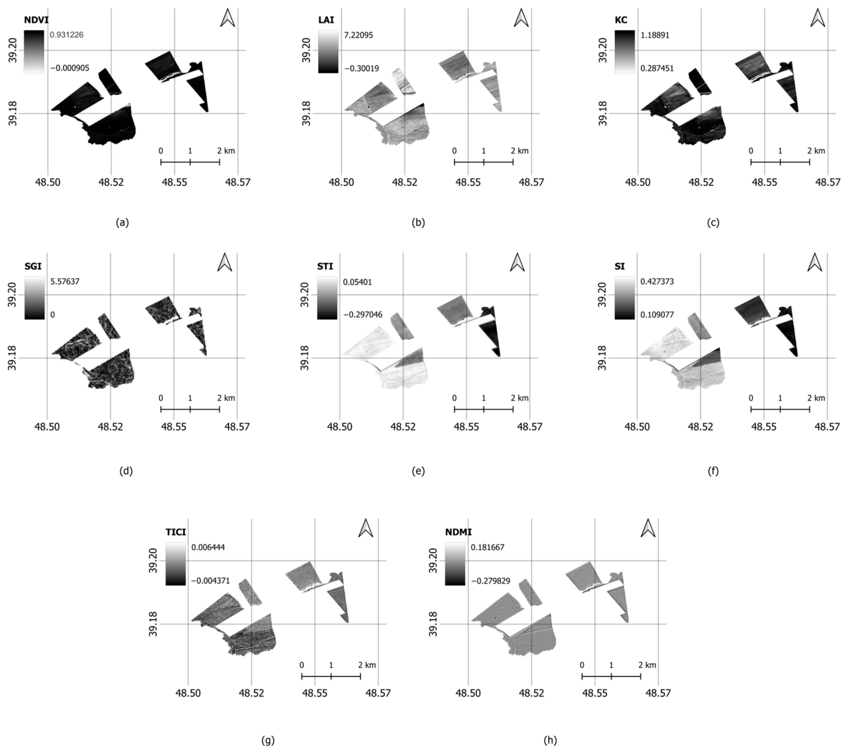
Two Sentinel 2 mosaic raster datasets containing green field and bare land imageries, also the SRTM DEM raster data were used to calculate several indices for this study.Green field imagery was used for calculating NDVI and LAI. Results are shown in Figure 4a,b. By using Sentinel 2 raster data, several SQ indices were calculated as shown in Figure 4e–h. SRTM data is used for calculating SGI (Figure 4d). The index results obtained from the calculations with various intervals are shown below.
In this study, NDVI results were obtained in the range of ~0 to ~1. Usually, NDVI values range from −1 to 1 [22]. As seen in Figure 4a, the NDVI values of AOI generally show a high trend.
LAI index usually ranges between ~0 and 10 [25]. Near 0 values indicate bare ground, while green leaves per area increase as the index value rises to ~10. As shown in Figure 4b, the green area of the AOI in this research was obtained in the range of ~−0.3 to ~7. Negative results can be considered as 0. KC index is calculated from the LAI, thus, its’ values start from [23].
The slope gradient is obtained from 0 to ~5 percent in this study. Usually, it ranges between 0 to 100. Variations between 0 to 3 indicate little or no slope, while 4 to 9 are accepted as gentle slopes [42].
The coefficient for the STI usually ranges between −1 (very poor) to 1 (excellent) [32]. Band 10 with a 1373.5 nm wavelength and Band 11 with a 1613.7 nm wavelength were obtained by correcting Sentinel 2 Level 1 data using the SNAP ESA Sen2Cor algorithm. As shown in Figure 4e, soil texture for the AOI in this study has moderate values.
Figure 4f shows high concentrations of saline soils for the AOI, as values above 0.2 indicate salinity in bare soils. Values between 0 to 0.19 show low or no salinity, while the maximum salinity value for this index is 1 [39].
As a result of calculations for determining total inorganic carbon compounds, we obtained moderate to low values in AOI as shown in Figure 4g as this index ranges from −1 (low) to 1 (high) [37].
The NDMI values range from −1 (low) to 1 (high), where the negative values correspond to low, while the positive values indicate high water/drainage content [35]. As shown in Figure 4h, soil moisture for the AOI in this study has low to moderate values.
Following the results shown in Figure 4, soil quality indices were later included in SQI calculation approaches. For this, indices multiplied with each other and were later calculated by the sixth root.
Using the Data plotting algorithm in QGIS, the correlation between the SQI and NDVI values has been visualized.
As shown in Figure 5, a non-linear scattered positive correlation between NDVI and SQI has been detected.
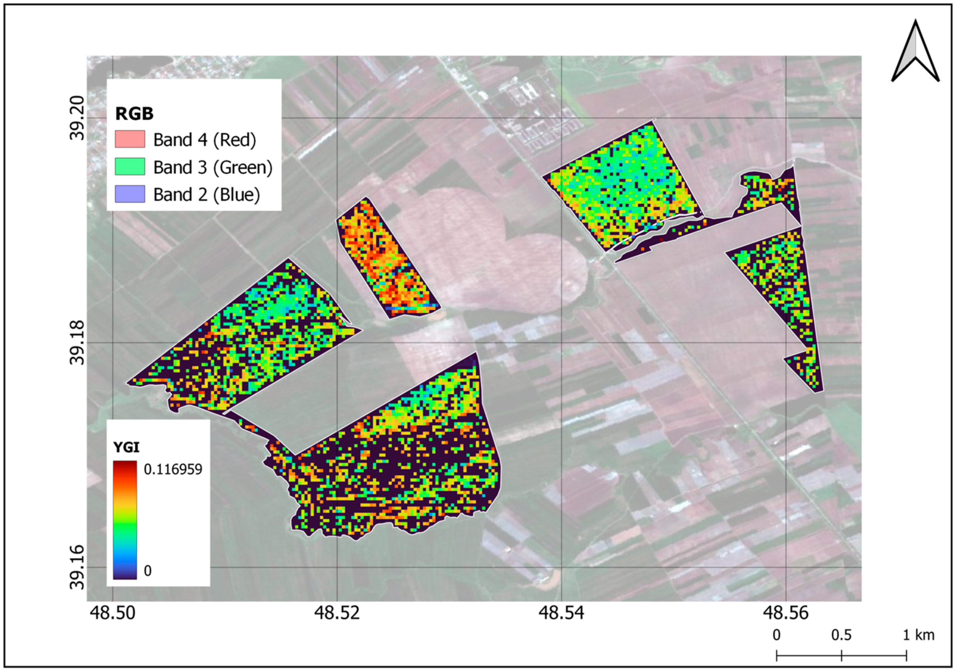
According to the results, the SQI rate varied between 0 to 1. Considerately, the Total Yield was calculated using the values shown in Figure 6. The yield gradient obtained using the MEDALUS method by multiplying SQI, NDVI, and the Kc indices is shown below.
To estimate the Total Yield of the given AOI, the mean value of the Yield gradient rate was multiplied by the total pixel count. Thus, unique value index reports were obtained with the total pixel count of 3637 using QGIS processing tools. Actual data reported by the official sources were 1103.2 tonnes. The indications are shown in Table 1.
On crop production, Mamatkulov’s approach accounted for the effects of crop coefficient, photosynthesis, and SQ based on the MEDALUS method. According to numerous study sources, these two models have been applied with all parameters derived from satellite data. This method is also applicable to a large-scale dataset. Nevertheless, the rate of validity is highly dependent on field productivity [19].
Using indices such as SQI, Kc, and NDVI, the YGI formula was calculated and the Mean Value was multiplied by the area to estimate Total Yield in tonnes, as shown in Formula (2).
As a result of the calculations, ~1081.3 total yields in tonnes were estimated. The total yield we acquired from the official sources reported a yield of roughly around 1103.2 tonnes. The model we developed acquired low RMSPE (0.01985) by only using RS data and GIS applications.
In contrast, the Mamatkulov study’s findings showed that the formula for harvest calculation applied to highly productive farmland had a high accuracy of 96% by using RS data only for calculating NDVI and SI indices [19]. The accuracy of yield estimations was still high (85%) but significantly lower for low-productive agriculture with this method [19]. The remaining data were obtained from laboratory analyses.
Consequently, using only RS data and GIS methods, Mamatkulov’s approach this research is based on, and the MEDALUS model we modified—forecasted agricultural yield with the greatest of ease, considering high accuracy (98.03%), low cost, and high availability.
A non-linear positive correlation between NDVI and SQI has been detected. Thus, if SQI in the soil is showing high trends before the plantation, NDVI and therefore, LAI values are also going to be high.
Considering the approach in this article as an option, more detailed analyses in this field can be conducted using a wide range of data.
GIS and RS technologies can be valuable tools for addressing complex agricultural concerns. The primary reason for development is that modern techniques such as GIS and RS can contribute significantly to the management of timely, accurate, cost-effective, and repetitious agricultural data [43]. Modern agriculture can benefit greatly from the application of GIS and RS technologies for monitoring crop development, detecting afflicted areas, assessing soil quality status, estimating yields, and visualizing the actual topography of crop fields, among other spatial analyses.
5. Conclusions
Climate change and global warming are the main threats to our planet. It can cause several natural hazards such as sea level rise, flooding, wildfire, and drought which are the main reasons for the decrease in natural resources, migration, and unexpected economical loss. The sustainable development goals aim for climate resilience nature to increase the living standard of the human being. From this perspective, this study has aimed for reliable, low cost and accurate crop estimation based on field survey free and only based on open access remotely sensed imageries.
Conventional approaches relied on reports from the field. Those were time-consuming, infeasible in the field, and prone to substantial inaccuracies due to insufficient ground observations, resulting in inaccurate crop yield and crop area estimations. Methods of RS based on empirical-statistical models should be calibrated in other regions since factor weights vary by location and those that cannot be operated on a broad scale disregard the effect of other factors. On a wide scale, RS techniques based on the water-consuming equilibrium model can be implemented, but they disregard the influence of numerous aspects, such as solar radiation, soil content, and photosynthetic intensity.
Crop growth models were comprehensive models that considered the most influential parameters. They could be operated on a big scale but had plenty of agronomic specifics and various criteria. Consequently, it was expensive and time-consuming. The expectation is that the new approaches to be implemented based on the conclusions investigated within the scope of this article will lead to applications that can play a significant role in many aspects of our lives, including agriculture, ecology, and urban planning.
As a future study, we aim to exploit deep learning-based approaches to improve our results and to make ideas scalable for different areas. Deep learning-based approaches have shown promising results in various fields, including image recognition, natural language processing, and computer vision. In the field of remote sensing and agriculture, deep learning methods have been applied to crop classification and yield prediction, achieving high accuracy and reducing the need for ground observations. Deep learning methods can be applied to any open-source or automated data-source-based model for large-scale datasets and near the real-time automatically updated results.
As our method consists of only open-source Remote Sensing data, deep learning automated models can apply side factors such as Crop health, Global evapotranspiration, Normalized Difference Burned Ratio Index, etc. Therefore, future research in this field could explore the potential of deep learning-based approaches for improving crop estimation and expanding their scalability to different regions.
Author Contributions
Conceptualization, Nilufar Karimli and Mahmut Oğuz Selbesoğlu; methodology, Nilufar Karimli; software, N.K.; validation, Mahmut Oğuz Selbesoğlu and Nilufar Karimli; formal analysis, Nilufar Karimli; investigation, Nilufar Karimli; resources, Nilufar Karimli and Mahmut Oğuz Selbesoğlu; data curation, Nilufar Karimli; writing—original draft preparation, Nilufar Karimli; writing—review and editing, Mahmut Oğuz Selbesoğlu and Nilufar Karimli; visualization, Nilufar Karimli; supervision, Mahmut Oğuz Selbesoğlu; project administration, Mahmut Oğuz Selbesoğlu; funding acquisition, Mahmut Oğuz Selbesoğlu and Nilufar Karimli. All authors have read and agreed to the published version of the manuscript.
Funding
This research received no external funding.
Data Availability Statement
Datasets used in this research are fully available in open-source portals. Sentinel-2 data was obtained from Copernicus Open Access Hub (www.scihub.copernicus.eu accessed on 21 February 2023) while DEM was downloaded from the Open Access Earth Science Data Systems (ESDS) Program (www.urs.earthdata.nasa.gov accessed on 21 February 2023). Processes and calculations have been carried out only using community and open-source software such as SNAP ESA and QGIS. GEE academic login was used for non-commercial purposes to analyse NDVI Time Series.
Acknowledgments
The research presented in this paper is based on the original MSc. thesis study of the first author, conducted at Istanbul Technical University, Institute of Graduate School, supervised by Mahmut Oğuz Selbesoğlu. The field data report for yield results had been provided by the Ministry of Agriculture of the Republic of Azerbaijan. Special thanks to Leading scientist at Azerbaijan National Academy of Sciences Institute of Geology and Geophysics, Bahruz Ahadov and representative of the Agricultural Economics Research Centre under the Ministry of Agriculture of the Republic of Azerbaijan, Konul Mammadova for reviews, feedback, and data provide support.
Conflicts of Interest
The authors declare no conflict of interest.
References
- Ghosh, P.; Kumpatla, S. GIS Applications in Agriculture. In Geographic Information Systems and Applications in Coastal Studies, 1st ed.; Zhang, Y., Cheng, Q., Eds.; IntechOpen: London, UK, 2022. [Google Scholar] [CrossRef]
- Bao, K.; Padsala, R.; Coors, V.; Thrän, D.; Schröter, B. A GIS-Based Simulation Method for Regional Food Potential and Demand. Land 2021, 10, 880. [Google Scholar] [CrossRef]
- Jin, X.; Liu, S.; Baret, F.; Hemerlé, M.; Comar, A. Estimates of plant density of wheat crops at emergence from very low altitude UAV imagery. Remote Sens. Environ. 2017, 198, 105–114. [Google Scholar] [CrossRef] [Green Version]
- Ölkədə Kənd Təsərrüfatı Məhsullarının Yığımı Başa Çatıb. Azerbaijan-News. 2023. Available online: https://www.azerbaijan-news.az/az/posts/detail/olkede-kend-teserrufati-mehsullarinin-yigimi-basa-catib-1675119441 (accessed on 21 February 2023).
- Panda, S.S.; Ames, D.P.; Panigrahi, S. Application of vegetation indices for agricultural crop yield prediction using neural network techniques. Remote Sens. 2010, 2, 673–696. [Google Scholar] [CrossRef] [Green Version]
- Cachia, F. Guidelines for the Measurement of Productivity and Efficiency in Agriculture; FAO: Rome, Italy, 2018. [Google Scholar] [CrossRef]
- Jørgensen, S.E. Models as Instruments for Combination of Ecological Theory and Environmental Practice. Ecol. Model. 1994, 75–76, 5–20. [Google Scholar] [CrossRef]
- Reynolds, M.P.; Ginkel, M.; Ribaut, J.M. Avenues for Genetic Modification of Radiation Use Efficiency in Wheat. J. Exp. Bot. 2000, 51, 459–473. [Google Scholar] [CrossRef] [PubMed] [Green Version]
- Jayne, T.; Xu, Z.; Guan, Z.; Black, R. Factors influencing the profitability of fertilizer use on maize in Zambia. Agric. Econ. 2009, 40, 437–446. [Google Scholar] [CrossRef] [Green Version]
- Mo, X.; Liu, S.; Lin, Z.; Xu, Y.; Xiang, Y.; McVicar, T.R. Prediction of Crop Yield, Water Consumption and Water Use Efficiency with a Svat-Crop Growth Model Using Remotely Sensed Data on the North China Plain. Ecol. Model. 2005, 183, 301–322. [Google Scholar] [CrossRef]
- Morel, J.; Todoroff, P.; Bégué, A.; Bury, A.; Martiné, J.-F.; Petit, M. Toward a Satellite-Based System of Sugarcane Yield Estimation and Forecasting in Smallholder Farming Conditions: A Case Study on Reunion Island. Remote Sens. 2014, 6, 6620–6635. [Google Scholar] [CrossRef] [Green Version]
- Ma, C.; Liu, M.; Ding, F.; Li, C.; Cui, Y.; Chen, W.; Wang, Y. Wheat growth monitoring and yield estimation based on remote sensing data assimilation into the SAFY crop growth model. Sci. Rep. 2022, 12, 5473. [Google Scholar] [CrossRef]
- Meraj, G.; Kanga, S.; Ambadkar, A.; Kumar, P.; Singh, S.K.; Farooq, M.; Johnson, B.A.; Rai, A.; Sahu, N. Assessing the Yield of Wheat Using Satellite Remote Sensing-Based Machine Learning Algorithms and Simulation Modeling. Remote Sens. 2022, 14, 3005. [Google Scholar] [CrossRef]
- Chullu, M. Estimation of the effect of soil salinity on crop yield using remote sensing and geographic information system. Turk. J. Agric. For. 2003, 27, 23–28. [Google Scholar]
- Arab, S.T.; Noguchi, R.; Matsushita, S.; Ahamed, T. Prediction of Grape Yields from Time-Series Vegetation Indices Using Satellite Remote Sensing and a Machine-Learning Approach. Remote Sens. Appl. Soc. Environ. 2021, 22, 100485. [Google Scholar] [CrossRef]
- AbdelRahman, M.A.E.; Saleh, A.M.; Arafat, S.M. Assessment of land suitability using a soil-indicator-based approach in a geomatics environment. Sci. Rep. 2022, 12, 18113. [Google Scholar] [CrossRef] [PubMed]
- Abbas, J. Assessment of land sensitivity to desertification for Al Mussaib project using MEDALUS approach. Casp. J. Environ. Sci. 2022, 20, 177–196. [Google Scholar] [CrossRef]
- Afzali, S.F.; Khanamani, A.; Maskooni, E.K.; Berndtsson, R. Quantitative Assessment of Environmental Sensitivity to Desertification Using the Modified MEDALUS Model in a Semi-arid Area. Sustainability 2021, 13, 7817. [Google Scholar] [CrossRef]
- Mamatkulov, Z.; Safarov, E.; Oymatov, R.; Abdurahmanov, I.; Rajapbaev, M. Application of GIS and RS in real-time crop monitoring and yield forecasting: A case study of cotton fields in low and high productive farmlands. In Proceedings of the Annual International Scientific Conference on Geoinformatics GI 2021: Supporting Sustainable Development by GIST, Tashkent, Uzbekistan, 27–29 January 2021; Volume 227. [Google Scholar] [CrossRef]
- Shokr, M.S.; Abdellatif, M.A.; El Baroudy, A.A.; Elnashar, A.; Ali, E.F.; Belal, A.A.; Attia, W.; Ahmed, M.; Aldosari, A.A.; Szantoi, Z.; et al. Development of a Spatial Model for Soil Quality Assessment under Arid and Semi-Arid Conditions. Sustainability 2021, 13, 2893. [Google Scholar] [CrossRef]
- Özer, G.; Paulitz, T.C.; Imren, M.; Alkan, M.; Muminjanov, H.; Dababat, A.A. Identity and Pathogenicity of Fungi Associated with Crown and Root Rot of Dryland Winter Wheat in Azerbaijan. Plant Dis. 2020, 104, 2149–2157. [Google Scholar] [CrossRef] [PubMed]
- Özyavuz, M. Analysis of Changes in Vegetation Using Multitemporal Satellite Imagery, the Case of Tekirdağ Coastal Town. J. Coast. Res. 2010, 26, 1038–1046. [Google Scholar] [CrossRef]
- El-Shirbeny, M.; Ali, A.; Saleh, N. Crop Water Requirements in Egypt Using Remote Sensing Techniques. J. Agric. Chem. Environ. 2014, 3, 57–65. [Google Scholar] [CrossRef] [Green Version]
- Beeri, O.; Netzer, Y.; Munitz, S.; Mintz, D.; Pelta, R.; Shilo, T.; Horesh, A.; Mey-tal, S. Kc and LAI Estimations Using Optical and SAR Remote Sensing Imagery for Vineyards Plots. Remote Sens. 2020, 12, 3478. [Google Scholar] [CrossRef]
- Najatishendi, E. Paddy-Rice Leaf Area Index (LAI) Estimation Using Radar and Optical Imagery; Bilişim Enstitüsü: Ankara, Türkiye, 2017; Available online: http://hdl.handle.net/11527/15726 (accessed on 12 October 2022).
- Su, Z.A.; Zhang, J.H.; Nie, X.J. Effect of Soil Erosion on Soil Properties and Crop Yields on Slopes in the Sichuan Basin, China. Pedosphere 2010, 20, 736–746. [Google Scholar] [CrossRef]
- Maurya, P.R.; Lal, R. Effects of No-Tillage and Ploughing on Roots of Maize and Leguminous Crops. Exp. Agric. 1980, 16, 185–193. [Google Scholar] [CrossRef]
- Kosmas, C.; Ferrara, A.; Briassouli, H.; Imeson, A. Manual on Key Indicators of Desertification and Mapping Environmentally Sensitive Areas to Desertification. In The Medalus Project: Mediterranean Desertification and Land Use; European Commission: Luxembourg, 1999; pp. 31–47. [Google Scholar]
- Nemes, A.; Timlin, D.J.; Pachepsky, Y.A.; Rawls, W.J. Evaluation of the Pedotransfer Functions for Their Applicability at the U.S. National Scale. Soil Sci. Soc. Am. J. 2009, 73, 1638–1645. [Google Scholar] [CrossRef]
- Makabe, S.; Kakuda, K.I.; Sasaki, Y.; Ando, T.; Fujii, H.; Ando, H. Relationship between Mineral Composition or Soil Texture and Available Silicon in Alluvial Paddy Soils on the Shounai Plain, Japan. Soil Sci. Plant Nutr. 2009, 55, 300–308. [Google Scholar] [CrossRef]
- Sullivan, J.M.; Twardowski, M.S.; Donaghay, P.L.; Freeman, S.A. Use of Optical Scattering to Discriminate Particle Types in Coastal Waters. Appl. Opt. 2005, 44, 1667. [Google Scholar] [CrossRef]
- Odeh, I.O.A.; McBratney, A.B. Using AVHRR Images for Spatial Prediction of Clay Content in the Lower Namoi Valley of Eastern Australia. Geoderma 2000, 97, 237–254. [Google Scholar] [CrossRef]
- Broll, G.; Brauckmann, H.J.; Overesch, M.; Junge, B.; Erber, C.; Milbert, G.; Baize, D.; Nachtergaele, F. Topsoil Characterization—Recommendations for Revision and Expansion of the FAO-Draft (1998) with Emphasis on Humus Forms and Biological Features. J. Plant Nutr. Soil Sci. 2006, 169, 453–461. [Google Scholar] [CrossRef]
- Məmmədov, Q.Ş. Azərbaycan Respublikası Torpaq Atlası; Elm: Baku, Azerbaijan, 2007; p. 127. [Google Scholar]
- Gao, B. NDWI—A Normalized Difference Water Index for Remote Sensing of Vegetation Liquid Water from Space. Remote Sens. Environ. 1996, 58, 257–266. [Google Scholar] [CrossRef]
- Ersoy, O.; Fidan, S.; Köse, H.; Güler, D.; Özdöver, Ö. Effect of Calcium Carbonate Particle Size on the Scratch Resistance of Rapid Alkyd-Based Wood Coatings. Coatings 2021, 11, 340. [Google Scholar] [CrossRef]
- Mitchell, C.; Hu, C.; Bowler, B.; Drapeau, D.; Balch, W.M. Estimating Particulate Inorganic Carbon Concentrations of the Global Ocean from Ocean Color Measurements Using a Reflectance Difference Approach. J. Geophys. Res. 2017, 122, 8707–8720. [Google Scholar] [CrossRef] [Green Version]
- Elhag, M.; Jarbou, A.B. Soil Salinity Mapping and Hydrological Drought Indices Assessment in Arid Environments Based on Remote Sensing Techniques. Geosci. Instrum. Methods Data Syst. 2017, 6, 149–158. [Google Scholar] [CrossRef] [Green Version]
- Allbed, A.; Lalit, K. Soil Salinity Mapping and Monitoring in Arid and Semi-Arid Regions Using Remote Sensing Technology: A Review. Adv. Remote Sens. 2013, 2, 373–385. [Google Scholar] [CrossRef] [Green Version]
- Prodanović, D.; Stanić, M.; Milivojević, V.; Simić, Z.; Arsić, M. DEM-based GIS algorithms for automatic creation of hydrological models data. J. Serb. Soc. Comput. Mech. 2009, 3, 64–85. [Google Scholar]
- Hyndman, R.J. Another Look at Forecast Accuracy Metrics for Intermittent Demand. Foresight Int. J. Appl. Forecast. 2006, 4, 43–46. [Google Scholar]
- Shields, D.H.; Harrington, E.J. Measurements of slope movements with a simple camera. In Proceedings of the Landslides Proceedings of the Fifth International Symposium, Lausanne, Switzerland, 10–15 July 1988; A.A. Balkema: Rotterdam, The Netherlands, 1988; pp. 521–525. [Google Scholar]
- Kingra, P.K.; Majumder, D.; Singh, S.P. Application of Remote Sensing and Gis in Agriculture and Natural Resource Management under Changing Climatic Conditions. Agric. Res. J. 2016, 53, 295–302. [Google Scholar] [CrossRef]
Figure 1.
Details of the test area. (a) Economic regions of Azerbaijan; (b) Natural Red Blue Green (RGB) band combination of Jalilabad, test area highlighted; (c) 2021–2022 NDVI time series analysis of the study area, created using Google Earth Engine (GEE), (d) Natural Red Blue Green (RGB) band combination of the test area highlighted.

Figure 2.
The Area of Interest (AOI) Sentinel-2 raster data as (a) RGB combination, bare soil; (b) False Infra-Red (FIR) combination, bare soil; (c) RGB combination, green field; (d) FIR combination, green field.
Figure 2.
The Area of Interest (AOI) Sentinel-2 raster data as (a) RGB combination, bare soil; (b) False Infra-Red (FIR) combination, bare soil; (c) RGB combination, green field; (d) FIR combination, green field.

Figure 3.
AOI from SRTM 30m resolution DEM.

Figure 4.
Calculated indices: (a) NDVI; (b) LAI; (c) KC; (d) SGI; (e) STI; (f) SI; (g) TICI; (h) NDMI.
Figure 4.
Calculated indices: (a) NDVI; (b) LAI; (c) KC; (d) SGI; (e) STI; (f) SI; (g) TICI; (h) NDMI.

Figure 5.
Correlation between NDVI and SQI.

Figure 6.
Yield gradient using TICI.


Table 1.
Total Yield, Validity rate, and RMSE are shown in the table.
| YIELDmean | |
|---|---|
| Ymean | 0.029730528 |
| Pixel count | 3637 |
| Ytotal, tonnes | 1081.299 |
| RMSPE, % | 1.985 |
| ValidityYmean, % | 98.0326 |
Disclaimer/Publisher’s Note: The statements, opinions and data contained in all publications are solely those of the individual author(s) and contributor(s) and not of MDPI and/or the editor(s). MDPI and/or the editor(s) disclaim responsibility for any injury to people or property resulting from any ideas, methods, instructions or products referred to in the content. |
© 2023 by the authors. Licensee MDPI, Basel, Switzerland. This article is an open access article distributed under the terms and conditions of the Creative Commons Attribution (CC BY) license (https://creativecommons.org/licenses/by/4.0/).
Share and Cite
MDPI and ACS Style
Karimli, N.; Selbesoğlu, M.O. Remote Sensing-Based Yield Estimation of Winter Wheat Using Vegetation and Soil Indices in Jalilabad, Azerbaijan. ISPRS Int. J. Geo-Inf. 2023, 12, 124. https://doi.org/10.3390/ijgi12030124
AMA Style
Karimli N, Selbesoğlu MO. Remote Sensing-Based Yield Estimation of Winter Wheat Using Vegetation and Soil Indices in Jalilabad, Azerbaijan. ISPRS International Journal of Geo-Information. 2023; 12(3):124. https://doi.org/10.3390/ijgi12030124
Chicago/Turabian StyleKarimli, Nilufar, and Mahmut Oğuz Selbesoğlu. 2023. "Remote Sensing-Based Yield Estimation of Winter Wheat Using Vegetation and Soil Indices in Jalilabad, Azerbaijan" ISPRS International Journal of Geo-Information 12, no. 3: 124. https://doi.org/10.3390/ijgi12030124
Note that from the first issue of 2016, this journal uses article numbers instead of page numbers. See further details here.