Testing Efficiency of the London Metal Exchange: New Evidence


1
Commodity Research Center, Public Procurement Service, Daejeon 35208, Korea
2
Housing Finance Research Institute, Korea Housing Finance Corporation, Busan 48400, Korea
*
Author to whom correspondence should be addressed.
Int. J. Financial Stud. 2018, 6(1), 32; https://doi.org/10.3390/ijfs6010032
Submission received: 26 December 2017
/
Revised: 27 February 2018
/
Accepted: 12 March 2018
/
Published: 14 March 2018
Abstract
:This paper explores the market efficiency of the six base metals traded on the LME (London Metal Exchange) using daily data from January 2000 to June 2016. The hypothesis that futures prices 3M (3-month) are unbiased predictors of spot prices (cash) in the LME is rejected based on the false premise that the financialization of commodities has been growing. For the robustness check, monthly data is analyzed using ordinary least squares (OLS) and GARCH (1,1) models. We reject the null hypothesis for all metals except for zinc.
JEL Classification:
C3; G11. Introduction
After the publication of Fama’s seminal paper (Fama 1970), the efficient market hypothesis (EMH) has been tested extensively in various asset markets such as the equity, currency (Hansen and Hodrick 1980), and even commodity (Beck 1994) markets and their derivatives. The EMH is a joint hypothesis that tests whether market participants can generate excess returns, and uses their expectations based on the rational expectations hypothesis.
The commodity futures market is an instrument that producers/farmers and traders can use to reduce their price risk. The commodity futures market is comprised of spot and futures prices, so the prices in the two respective markets become the main measures of market efficiency (Gross 1988; Goss 1981). A futures price reflects the expectation of market participants. One way to test the EMH is to determine whether the futures price is the unbiased estimator of the future spot price . Note that the futures price at time t for a contract with maturity length n is an unbiased predictor of the spot price as long as the hypothesis prevails in the market at time t + n. If the EMH holds, the forecast error has a mean of zero and is serially uncorrelated.
The London Metal Exchange (LME) is the world’s largest futures exchange in the metal industry, and addresses mainly base metals (non-ferrous) and other metals. The LME provides spot (cash), futures (3M), and various option contracts for the six base metals. The LME addresses daily rolling 3-month (3M) futures contracts that are different from those in other commodity markets, which are based on monthly prompt dates. The LME is traded electronically, but in particular, is also traded through the open outcry, which is the oldest way of trading on the exchange. Ring1 trading is the LME’s way of open outcry. The official prices are established by the second ring in the morning session, which is treated as the benchmark for industry supply and demand, while financial investors focus instead on the closing prices. These characteristics are somewhat different from other asset markets, which can possibly impact the LME’s volatility process (Figuerola-Ferretti and Gilbert 2008). The purpose of this paper is to reexamine the market efficiency of the LME in terms of Canarella and Pollard’s investigative framework (1986) and considers the updated data to reflect the effect of commodity financialization (Cheng and Xiong 2014). Canarella and Pollard analyzed the market efficiency of the LME through monthly data from January 1975 to December 1983 found that the 3M futures price was an unbiased estimator for the spot price. Cheng and Xiong (2014) noted that commodity financialization resulted in somewhat higher price volatility due to the large inflow of investment money to the commodity futures markets. This phenomenon led to regulators’ concerns that financialization distorted commodity prices. On the data verification front, the data used in Canarella and Pollard (1986) were from an old-fashioned method of collecting monthly data by hand from the Wall Street Journal. Sephton and Cochrane (1990) relied on various sources, such as the New York Times, the Times, and the Globe and Mail, though they still collected data by hand. This paper used daily data from Reuters, which provides high frequency data compared to monthly data. While Canarella and Pollard (1986) studied four base metals, we examined the six base metals that are the main trading commodities on the LME. The empirical results suggest that the LME futures market is inefficient, which can generate somewhat possible excess returns. Through the robustness checks using monthly data, our empirical findings regarding the EMH of the LME’s base metals remained unchanged except for zinc.
2. Literature Review
There has not been regarding about the market efficiency of the LME. Canarella and Pollard (1986), Gross (1988), and MacDonald and Taylor (1988) found that the LME was efficient, while Kenourgios and Samitas (2004) and Otto (2011) found opposing results.
Goss (1985) tested the joint hypothesis of spot and futures prices on the LME from 1966 to 1984. He rejected the EMH for copper and zinc, but not for lead and tin. Sephton and Cochrane (1990) investigated the EMH for the LME with respect to six major base metals using monthly overlapping data from 1976 to 1989. They found that the LME is an inefficient market. Sephton and Cochrane (1991) reconsidered the LME data over the same period using the CUSUM of Squares stability test. They showed that the LME experienced structural change over this period, which implied that the market efficiency tests based on the Fama research scheme were somewhat less than conclusive (Sephton and Cochrane 1990).
In a seminal paper, Canarella and Pollard (1986) examined data for the four base metals (copper, lead, zinc, and tin) from January 1975 to December 1983. They utilized monthly, non-overlapping data and overlapping observations. The ordinary least squares (OLS) model was applied to non-overlapping data, while an autoregressive moving average (ARMA) process was applied to the error terms used in overlapping data. For both non-overlapping and overlapping data, they found that the hypothesis of market efficiency was not statistically rejected. This implied that the futures prices were unbiased predictors of the respective future spot prices. Any strategy, therefore, designed to enhance the long-term profitability of trading LME futures may not succeed as long as the market is efficient.
Gross (1988) tested the semi-strong EMH for copper and aluminum from 1983 to 1984 using the mean square error criterion. He found that the semi-strong EMH could not be rejected for both base metals.
MacDonald and Taylor (1988) analyzed the EMH of the LME using a test for cointegration on data from 1976–1987. They found that the EMH could not be rejected for copper and lead, but could be rejected for tin and zinc. In line with the cointegration method, Kenourgios and Samitas (2004) explored the 3-month and 15-month maturities of copper futures contracts from 1989 to 2000 found that the copper futures market was not efficient. Using the cointegration approach, Arouri et al. (2011) studied aluminum on the LME and investigated both short- and long-run efficiency, and they showed that the futures aluminum price was cointegrated with the spot price, which was then a biased estimator of the future spot price.
Otto (2011) analyzed the EMH of the LME using 3M (the most liquid futures contract on the LME) and 15-month (15M) futures prices from July 1991 to March 2008 with the monthly average second ring price data. He rejected the null hypothesis of speculative efficiency for all base metals with the exception of aluminum. He argued that one reason for aluminum’s efficiency may have been due to aluminum being the most liquid on the LME. For the 15M contracts, he failed to reject the null hypothesis for the six major base metals except for lead and tin. He noted that a possible reason for rejecting the hypothesis for lead and tin is in their illiquidity. Due mainly to trading reality, brokers usually calculate the futures prices based on the most liquid 3M futures contract prices (Otto 2011). Using the 15M futures prices to analyze the EMH seems to be irrelevant. As the concept of market efficiency seems to require somewhat sufficient liquidity, the 15-month tenor data analysis cannot satisfy the principles of arbitrage. Thus, this paper focused on 3M futures rather than 15M futures.
Chinn and Coibion (2014) investigated the unbiasedness of futures prices in major commodity markets such as energy, precious metals, base metals, and agricultural commodities using the statistical relationship between the basis and ex-post price changes. In particular, they considered the major base metals aluminum, copper, lead, nickel, and tin (not zinc) through Bloomberg. The monthly data they used in their study started in July 1997. They found that the futures prices of precious and base metals implied a strong rejection of the null hypothesis of unbiasedness, while the futures prices in the energy and agricultural markets were consistent with unbiasedness.
In summary, there is no consensus regarding the efficiency of the LME. Some studies have been criticized for using incorrect econometric methodology (Otto 2011). Furthermore, most studies have utilized monthly data, which cannot appropriately capture the arbitrage possibilities in the futures markets. In particular, there has been some discussion regarding how average data may lead to spurious results (Gross 1988). This paper therefore applied the proven Canarella and Pollard (1986) methodology to recent and somewhat high-frequency data, or daily data, to reflect the market arbitrage possibilities that institutional investors face.
3. Research Design
3.1. Regression Model
The purpose of this paper was to examine whether the futures prices on the LME are unbiased predictors. Canarella and Pollard (1986) utilized monthly non-overlapping observations to test the LME’s efficiency using the following regression model in Equation (1):
where is the natural logarithm of the spot price; and is the natural logarithm of the three-month futures price. The statistically insignificant coefficient of 0 for and 1 for would render the futures price an unbiased predictor of the spot price (Gross 1988). Notice that if the formal joint hypothesis, and does not hold, the futures price is an unbiased estimator of the future spot price. The implication of the efficient market hypothesis is that the futures price is the best forecast of the spot price. As a joint hypothesis, the formal Wald test was employed in this paper.
3.2. Data and Sample Construction
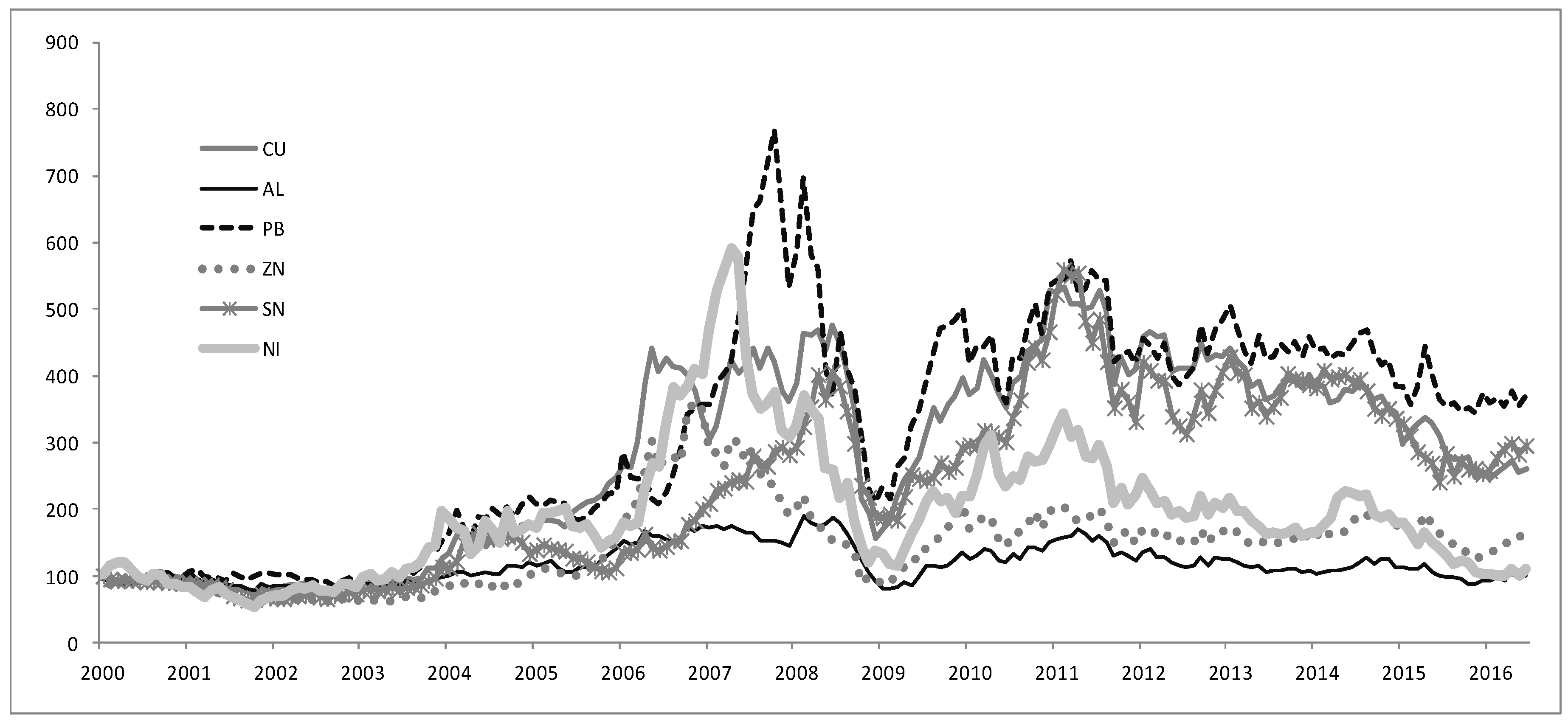
Since commodities were first considered an alternative asset class2 in the market starting in 2000 (Cheng and Xiong 2014), this paper analyzed the period after 2000, providing N = 3285 daily non-overlapping observations3 through Reuters. Within the sample period, the commodities market faced a bull market driven by the massive Chinese capital expenditure (CAPEX) demands and a severe bear market due mainly to the bankruptcy of the Lehman Brothers. The empirical results seem to be robust because of the market dynamics. Figure 1 plots the normalization of the spot prices of the six base metals starting January 2000, which indicates the boom and bust in the LME within the dataset. Notice that the price fluctuation of lead was somewhat larger when compared to others with its highest data point of 769.69 in October 2007 and its lowest data point of 211.49 in December 2008 due to the global financial crisis. Once again, the price of lead surged to 558.20 in June 2011. On the other hand, aluminum experienced a somewhat smoother price fluctuation, where it reached 188.64 in February 2008 but fell to 80.4 in February 2009. The changes in aluminum price were subdued when compared to other metals on the LME (Chinn and Coibion 2014).
In general, the base metals exhibited strong comovement with one another and somewhat higher volatility across the board mainly due to the global financial crisis driven by the Lehman bankruptcy (Tang and Xiong 2012).
Using Reuters, the data for the spot price and the 3M futures price were collected and construed as the prices at close of the second ring in afternoon trading, which is the official price the LME board approves.
4. Empirical Results
4.1. Regression Results
If (1) investors are risk neutral; (2) the costs of transaction are negligible; (3) information is applied rationally; and (4) the market is competitive, then the market is efficient, and the expected rate of return to speculation in the futures market will be zero. Note that, if the futures price is an unbiased estimator of the future spot price, the constant () should differ insignificantly from zero, and the coefficient on the futures price should differ insignificantly from unity. These conditions are critical for the EMH.
Using non-overlapping daily data, Table 1 shows the regression results of OLS, which presents the model’s coefficients with t-ratios. The constants had a range of 0.31 ~ 0.91, which were statistically significant with a 1% significance level. The coefficients on the futures price also revealed the range of 0.87 ~ 0.97, which was also statistically significant with a 1% significance level. The empirical results were different from the above hypothesis of and with statistical insignificance, while the regression analysis suggests somewhat similar results across base metals. In addition, the values are all high across the regression results for the base metals.
4.2. The Joint Hypothesis Test
It is important to remember that the rejection of the null hypothesis is a formal rejection of the hypothesis of market efficiency in finance and of unbiased expectations in econometrics. The joint hypothesis for the LME efficiency was tested by the formal Wald test, which tests whether an independent variable has a statistically significant relationship with a dependent variable. The F-test statistic is
where is the restricted sum of squared residuals, is the unrestricted sum of squared residuals, q is the number of restrictions implied, N is the number of observations, and k is the total unrestricted number of parameters.
Table 2 exhibits the test statistics for testing the joint hypothesis . The hypothesis proposed was the EMH, which suggested that the futures price was the best predictor of the future spot price. Table 2 clearly illustrates that the LME was inefficient. The F-test statistics were statistically significant with a 1% significance level, and those results were very similar to those from the regression analysis. The rejection of the joint hypothesis means that the LME was not an efficient market, which means that the market prices did not fully reflect all currently available information (Fama 1970). Some informed traders in the market can therefore make an abnormal return with private information. These findings did not coincide with former studies, except for those by Sephton and Cochrane (1990). They stated that the reason may be related to time-varying risk premia. Due mainly to the collapse of Lehman Brothers, which was driven by the global financial crisis, the somewhat synchronized boom and bust cycle4 in approximately 2008 caused the price volatility of many commodities to spike (Cheng and Xiong 2014).
This paper examined whether the price volatility of the LME changed within a sample period to check the possibility of time-varying volatility due to the financialization of commodity markets. Table 3 shows the results from the difference-in-means tests of volatility difference in two sub-periods: pre-crisis (2000 ~ 2008) and post-crisis (2009 ~ June 2016). It was found that the LME’s volatility was somewhat larger post-crisis when compared to pre-crisis with a statistical significance of 1% for all base metals, except for nickel. The somewhat serious inflow of investment money to the LME futures market as financialization has substantially changed amidst larger volatility, which seems to have had an impact on the LME market efficiency phenomenon. Indeed, Park (2017) constructed two hypotheses concerning whether the investment flows of money managers impacted the base metal prices and volatilities. He found that money managers’ speculative investment changes led LME metal prices and increased the volatilities.
LME could be inefficient due to the open outcry trading method and the daily rolling three-month prompt dates. In the market for oil and gold, the usual monthly prompt dates can be found. However, the LME uses a different structure such as electronic trading with the open outcry trading method and the daily rolling 3M prompt date. Those factors can motivate investments in the LME to generate excess returns. In addition, somewhat higher price volatility in the LME seems to render the market inefficient.
Chinn and Coibion (2014) found that the predictive power of commodity futures prices has gradually decreased since the early 2000s. They noted that the financialization of commodity markets through institutional investors’ index funds such as pension funds, was one reason behind this trend. This financialization could potentially reflect a number of factors such as changing risk premiums following the global financial crisis or increasing financial investments into commodity futures. Cheng et al. (2015) reported that the risk premiums varied over time as the financial investors’ risk bearing capacity is time varying.
4.3. Robustness Tests
To ensure the robustness of the empirical results in this paper, we performed two robustness checks. First, we analyzed monthly data and compared it with the results of daily data within the same period using OLS, which focuses on end-of-month values, rather than using monthly average data, for each base metal’s futures price. The coefficients of the 3M futures price in Table 4 coincide with the results in Table 1, which revealed a range of 0.88 ~ 0.97 with a statistical significance of 1%. In general, the regression results suggested somewhat similar results across the base metals. For the 3M contracts, we rejected the null hypothesis for all but zinc based on the Wald test, the results of which are given in Table 5. It was found that the zinc futures price was the best predictor of the future spot price.
Second, the GARCH (1,1) model as an alternative methodology, applies to Equation (1) the same monthly data to check the robustness of the previous results for comparison. This time, the estimates of the 3M futures prices were very similar to previous results within the range of 0.88 ~ 0.96 and a statistical significance of 1% in Table 6. However, the Wald test results in Table 7 were slightly less powered in terms of statistically significant levels, which meant that there should be less robust rejections of market efficiency than previous results indicated. Based on the F-test statistics, only aluminum was statistically significant with a 1% significance level, while nickel showed 5% significance, and copper, lead, and tin only had 10% significance. The testing power was somewhat lower when compared to previous testing results. The zinc futures price failed to reject the null hypothesis and hence was an unbiased estimator.
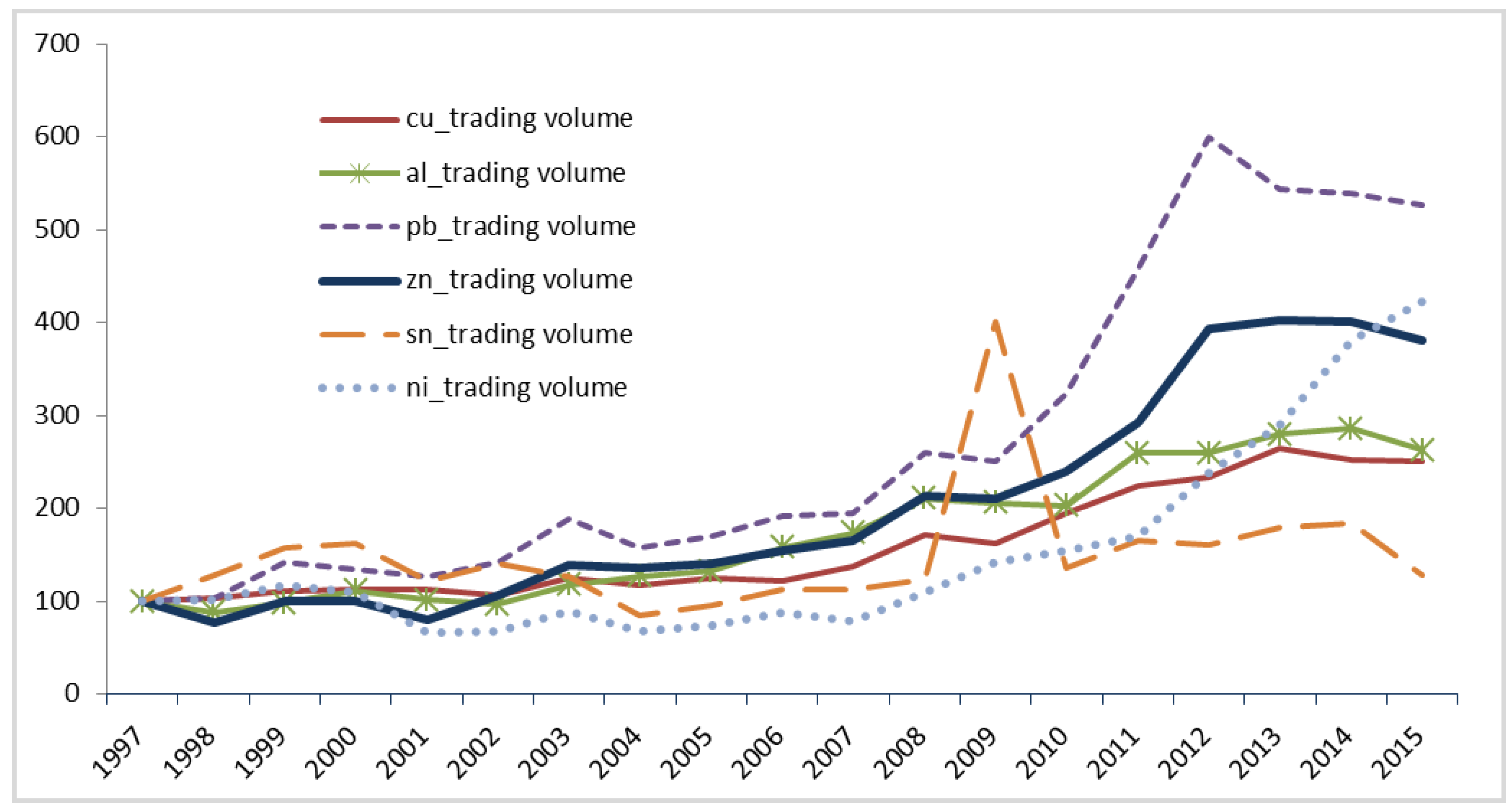
In general, through the robustness checks, our empirical findings regarding the EMH of the LME’s base metals remained unchanged except for zinc. Now, the question may arise as to why the Wald test results of zinc were different on the monthly data front. One possibility might be that the trading volume diverged, as Otto (2011) has argued, and the possible reason for rejection might be illiquidity. We therefore considered the trading volume trend since 1997 to identify how the trading volume of zinc strengthened when compared to other base metals. Figure 2 plots the normalization of the trading volume for the six base metals in terms of total annual trading volume starting from 1997. It was found that there are some trading volume divergences within the six base metals and that zinc, except for recent surges in nickel, has the second largest over the period. Unlike other base metals, zinc has a dominant production company, Glencore. Its market share of total global production is more than 50% according to the Bloomberg data, so this characteristic seems to play a role in market efficiency.
5. Summary and Conclusions
The futures market of the LME has raised the question of whether the base metals’ price information incorporates future movements in spot prices to identify the EMH. In this paper, we analyzed the recent period from 2000 to June 2016 and used daily non-overlapping observations to identify the market efficiency of the LME. The findings suggested that the LME was not an efficient market within the Canarella and Pollard (1986) framework. Hence, the LME can attract speculators such as hedge funds managers and CTAs (commodity trading advisors). Interesting explanations of inefficiency include the financialization of the commodity markets through the growth of index funds (Cheng and Xiong 2014). For the robustness check, we examined the end-of-month price data for each LME futures price within the same period using the OLS and GARCH (1,1) models. While there remains some room for debate over zinc, the other base metals revealed an inefficient market, which was consistent with the results of the daily data analysis.
Further studies regarding market efficiency of the LME should focus on the different interactions with other major commodity markets such as the New York Mercantile Exchange and the Shanghai Metal Exchange.
Author Contributions
Jaehwan Park conceived and developed the research design. Byungkwon Lim collected, analyzed the data and gave useful comments.
Conflicts of Interest
The authors declare no conflicts of interest.
References
- Arouri, Mohamed El Hedi, Fredj Jawadi, and Prosper Mouak. 2011. The Speculative Efficiency of the Aluminum Market: A Nonlinear Investigation. International Economics 126–27: 73–89. [Google Scholar] [CrossRef]
- Beck, Stacie E. 1994. Cointegration and Market Efficiency in Commodities Futures Markets. Applied Economics 26: 249–57. [Google Scholar] [CrossRef]
- Canarella, Giorgio, and Stephen K. Pollard. 1986. The “Efficiency” of the London Metal Exchange: A Test with Overlapping and Non-Overlapping Data. Journal of Banking and Finance 10: 575–93. [Google Scholar] [CrossRef]
- Cheng, Ing-Haw, and Wei Xiong. 2014. Financialization of Commodity Markets. Annual Review of Financial Economics 6: 419–41. [Google Scholar] [CrossRef]
- Cheng, Ing-Haw, Andrei Kirilenko, and Wei Xiong. 2015. Convective Risk Flows in Commodity Futures Markets. Review of Finance 19: 1733–81. [Google Scholar] [CrossRef]
- Chinn, Menzie D., and Olivier Coibion. 2014. The Predictive Content of Commodity Futures. The Journal of Futures Markets 34: 607–636. [Google Scholar] [CrossRef]
- Ewing, Bradley T., and Farooq Malik. 2013. Volatility Transmission between Gold and Oil Futures under Structural Breaks. International Review of Economics and Finance 25: 113–21. [Google Scholar] [CrossRef]
- Fama, Eugene F. 1970. Efficient Capital Markets: A Review of Theory and Empirical Work. Journal of Finance 25: 383–417. [Google Scholar] [CrossRef]
- Figuerola-Ferretti, Isabel, and Christopher L. Gilbert. 2008. Commonality in the LME Aluminum and Copper Volatility Processes through a FIGARCH Lens. The Journal of Futures Markets 28: 935–62. [Google Scholar] [CrossRef]
- Goss, Barry A. 1981. The Forward Pricing Function of the London Metal Exchange. Applied Economics 13: 133–50. [Google Scholar] [CrossRef]
- Goss, Barry A., ed. 1985. The Forward Pricing Function of the London Metal Exchange. In Futures Markets: Their Establishment and Performance. London: Routledge, pp. 157–73. [Google Scholar]
- Gross, Martin. 1988. A Semi-Strong Test of the Efficiency of the Aluminum and Copper Markets at the LME. The Journal of Futures Markets 8: 67–77. [Google Scholar] [CrossRef]
- Hansen, Lars Peter, and Robert J. Hodrick. 1980. Forward Exchange Rates as Optimal Predictors of Spot Rates: An Econometric Analysis. Journal of Political Economy 88: 829–53. [Google Scholar] [CrossRef]
- Kenourgios, Dimitris, and Aristeidis Samitas. 2004. Testing Efficiency of the Copper Futures Market: New Evidence from London Metal Exchange. Global Business and Economics Review, Anthology. pp. 261–71. Available online: https://papers.ssrn.com/sol3/papers.cfm?abstract_id=869390 (accessed on 27 February 2018).
- MacDonald, Ronald, and Mark Taylor. 1988. Metal Prices, Efficiency and Cointegration: Some Evidence from the LME. Bulletin of Economic Research 40: 235–39. [Google Scholar] [CrossRef]
- Otto, Sascha Werner. 2011. A Speculative Efficiency Analysis of the London Metal Exchange in a Multi-Contract Framework. International Journal of Economics and Finance 3: 3–16. [Google Scholar] [CrossRef]
- Park, Jaehwan. 2017. Effect of Speculators’ Position Changes in the LME Futures Market, Working Paper, under review.
- Park, Jaehwan. 2018. Volatility Transmission between Oil and LME Futures. Applied Economics and Finance 5: 65–72. [Google Scholar] [CrossRef]
- Sephton, Peter S., and Donald K. Cochrane. 1990. A Note of the Efficiency of the London Metal Exchange. Economic Letters 33: 341–45. [Google Scholar] [CrossRef]
- Sephton, Peter S., and Donald K. Cochrane. 1991. The Efficiency of the London Metal Exchange: Another Look at the Evidence. Applied Economics 23: 669–74. [Google Scholar] [CrossRef]
- Tang, Ke, and Wei Xiong. 2012. Index Investment and the Financialization of Commodities. Financial Analysts Journal 68: 54–74. [Google Scholar] [CrossRef]
| 1 | The official settlement price is determined by each metal trading session. Each metal trading session is signaled by a bell sound, so the LME open outcry is called the ring market. |
| 2 | Cheng and Xiong (2014) argued that commodity futures had become an important asset class for portfolio investors, much like stocks and bonds over the past decade. According to the CFTC’s (Commodity Futures Trading Commission) paper in 2008, investment money inflow rapidly increased to various commodity futures indices from early 2000 to 30 June 2008, totaling $200 billion. |
| 3 | The LME provides daily spot and 3-month futures prices. To test market efficiency, we can construct non-overlapping observations. This means spot price at time t and lagged t − 3 month futures price. This was obtained by mapping the synchrony between the sampling period and the contract period (see details in Canarella and Pollard (1986)). |
| 4 | Ewing and Malik (2013) found the linkage that existed between the volatilities in oil and gold, while Park (2018) found evidence of volatility transmission between oil and base metals thanks to the financialization of the commodity markets. This evidence suggests that there was a somewhat synchronized boom and bust cycle within the commodities. |
Figure 1.
Plot of base metal prices (normalized by their January 2000 value).

Figure 2.
Plot of base metal trading volume (normalized by their 1997 values).


Table 1.
Ordinary least squares (OLS) parameter estimates of Equation (1): daily data analysis.
| Commodity | F-Value | MSE | |||
|---|---|---|---|---|---|
| Aluminum | 0.91 | 0.87 | 0.77 | 11,220 | 0.10 |
| (14.5) | (105.9) | ||||
| Copper | 0.39 | 0.95 | 0.93 | 46,716 | 0.15 |
| (10.7) | (216.1) | ||||
| Lead | 0.36 | 0.95 | 0.93 | 44,384 | 0.16 |
| (11.1) | (210.6) | ||||
| Zinc | 0.35 | 0.95 | 0.89 | 26,991 | 0.15 |
| (8.22) | (164.3) | ||||
| Tin | 0.31 | 0.97 | 0.94 | 56,226 | 0.14 |
| (8.04) | (237.1) | ||||
| Nickel | 0.70 | 0.93 | 0.85 | 18,827 | 0.19 |
| (10.9) | (137.2) |
Notes: The total observation contained 3285 obs. (January 2000 ~ June 2016; daily data). The natural logarithm data were applied in equation estimation. The t-ratios are in parenthesis. To test the LME’s efficiency, the following regression model was used: , where is the spot price, and is the three-month futures price. The statistically insignificant coefficient of 0 for and 1 for would render the futures price an unbiased predictor of the spot price.
Table 2.
Joint hypothesis testing: daily data analysis.
| Statistics | Aluminum | Copper | Lead | Zinc | Tin | Nickel |
|---|---|---|---|---|---|---|
| F-statistic | 125.8 | 70.9 | 76.9 | 34.9 | 53.1 | 59.3 |
| p-value | 0.00 | 0.00 | 0.00 | 0.00 | 0.00 | 0.00 |
Notes: The testing joint hypothesis: . None of the F-tests were insignificant at the 1% level.
Table 3.
Difference tests of daily volatilities for pre-crisis (2000–2008) vs. post-crisis (2009–June 2016).
Table 3.
Difference tests of daily volatilities for pre-crisis (2000–2008) vs. post-crisis (2009–June 2016).
| Variables | Pre-Crisis | Post-Crisis | Difference Tests | |||
|---|---|---|---|---|---|---|
| Obs. | Pre-Mean | Obs. | Post-Mean | t-Stat. | p-Value | |
| Aluminum_abs. | 1483 | 0.902 | 1802 | 1.106 | 7.08 | 0.000 |
| Copper_abs. | 1483 | 1.149 | 1802 | 1.291 | 3.61 | 0.000 |
| Lead_abs. | 1483 | 1.295 | 1802 | 1.620 | 7.10 | 0.000 |
| Zinc_abs. | 1483 | 1.221 | 1802 | 1.491 | 6.41 | 0.000 |
| Tin_abs. | 1483 | 1.059 | 1802 | 1.340 | 6.75 | 0.000 |
| Nickel_abs. | 1483 | 1.741 | 1802 | 1.716 | −0.49 | 0.627 |
| Aluminum_sq. | 1483 | 1.502 | 1802 | 2.113 | 4.99 | 0.000 |
| Copper_sq. | 1483 | 2.573 | 1802 | 3.343 | 3.23 | 0.001 |
| Lead_sq. | 1483 | 3.183 | 1802 | 5.067 | 5.96 | 0.000 |
| Zinc_sq. | 1483 | 2.969 | 1802 | 4.138 | 4.66 | 0.000 |
| Tin_sq. | 1483 | 2.427 | 1802 | 3.779 | 4.82 | 0.000 |
| Nickel_sq. | 1483 | 5.540 | 1802 | 5.568 | 0.07 | 0.946 |
Notes: The volatilities were calculated as the absolute value of the daily returns. For example, Aluminum_abs. denotes the daily volatility of aluminum in absolute terms, while Aluminum_sq. represents that of aluminum in squared terms, respectively, which follows the Figuerola-Ferretti and Gilbert (2008) calculation method. The results showed that LME’s volatility was larger post-crisis when compared to pre-crisis.
Table 4.
OLS parameter estimates of Equation (1): monthly data analysis.
| Commodity | F-Value | MSE | |||
|---|---|---|---|---|---|
| Aluminum | 0.85 | 0.88 | 0.79 | 718.8 | 0.10 |
| (3.40) | (26.8) | ||||
| Copper | 0.39 | 0.95 | 0.93 | 2769 | 0.16 |
| (2.57) | (52.6) | ||||
| Lead | 0.36 | 0.95 | 0.93 | 2749 | 0.16 |
| (2.74) | (52.4) | ||||
| Zinc | 0.32 | 0.96 | 0.89 | 1680 | 0.14 |
| (1.86) | (40.9) | ||||
| Tin | 0.30 | 0.97 | 0.94 | 3592 | 0.14 |
| (2.00) | (59.9) | ||||
| Nickel | 0.65 | 0.93 | 0.86 | 1182 | 0.19 |
| (2.51) | (34.3) |
Notes: The total observation contained 195 obs. (January 2000 ~ June 2016; monthly data). The natural logarithm data were applied in equation estimation. The t-ratios are in parenthesis. To test the LME’s efficiency, the following regression model was used: , where is the spot price, and is the three-month futures price. The statistically insignificant coefficient of 0 for and 1 for would render the futures price an unbiased predictor of the spot price.
Table 5.
Joint hypothesis testing: monthly data analysis (OLS).
| Statistics | Aluminum | Copper | Lead | Zinc | Tin | Nickel |
|---|---|---|---|---|---|---|
| F-statistic | 6.76 | 4.44 | 4.86 | 1.75 | 3.32 | 3.18 |
| p-value | 0.00 | 0.00 | 0.00 | 0.18 | 0.03 | 0.04 |
Notes: The testing joint hypothesis: . The F-tests were statistically significant at the 1% level except for zinc. Tin and nickel were statistically significant at 5%.
Table 6.
GARCH parameter estimates of Equation (1): monthly data analysis.
| Commodity | Log Likelihood | |||
|---|---|---|---|---|
| Aluminum | 0.85 | 0.88 | 0.80 | 160.1 |
| (3.01) | (23.9) | |||
| Copper | 0.39 | 0.95 | 0.93 | 82.6 |
| (1.85) | (38.1) | |||
| Lead | 0.36 | 0.95 | 0.93 | 78.3 |
| (2.17) | (42.4) | |||
| Zinc | 0.32 | 0.96 | 0.88 | 100.8 |
| (1.56) | (35.1) | |||
| Tin | 0.30 | 0.96 | 0.94 | 104.6 |
| (1.74) | (52.8) | |||
| Nickel | 0.65 | 0.93 | 0.86 | 48.1 |
| (2.52) | (35.0) |
Notes: The total observation contains 195 obs. (January 2000 ~ June 2016; monthly data). The natural logarithm data were applied in equation estimation. The t-ratios are in parenthesis. GARCH (1,1) model was applied to project. To test the LME’s efficiency, the following regression model was used: , where is the spot price, and is the three-month futures price. The statistically insignificant coefficient of 0 for and 1 for would render the futures price an unbiased predictor of the spot price.
Table 7.
Joint hypothesis testing: monthly data analysis (GARCH).
| Statistics | Aluminum | Copper | Lead | Zinc | Tin | Nickel |
|---|---|---|---|---|---|---|
| F-statistic | 13.6 | 5.04 | 5.66 | 2.97 | 4.71 | 6.69 |
| p-value | 0.00 | 0.08 | 0.06 | 0.22 | 0.09 | 0.03 |
Notes: The testing joint hypothesis: . The F-test of aluminum was statistically significant at the 1% level. Nickel was statistically significant at 5%, while copper, lead, and tin were statistically significant at 10%. Zinc could not reject the null hypothesis.
© 2018 by the authors. Licensee MDPI, Basel, Switzerland. This article is an open access article distributed under the terms and conditions of the Creative Commons Attribution (CC BY) license (http://creativecommons.org/licenses/by/4.0/).
Share and Cite
MDPI and ACS Style
Park, J.; Lim, B. Testing Efficiency of the London Metal Exchange: New Evidence. Int. J. Financial Stud. 2018, 6, 32. https://doi.org/10.3390/ijfs6010032
AMA Style
Park J, Lim B. Testing Efficiency of the London Metal Exchange: New Evidence. International Journal of Financial Studies. 2018; 6(1):32. https://doi.org/10.3390/ijfs6010032
Chicago/Turabian StylePark, Jaehwan, and Byungkwon Lim. 2018. "Testing Efficiency of the London Metal Exchange: New Evidence" International Journal of Financial Studies 6, no. 1: 32. https://doi.org/10.3390/ijfs6010032
Note that from the first issue of 2016, this journal uses article numbers instead of page numbers. See further details here.