
Chemical-Mediated Microbial Interactions Can Reduce the Effectiveness of Time-Series-Based Inference of Ecological Interaction Networks

 , , ,
, , ,
Abstract
:1. Introduction
2. Materials and Methods
2.1. Models
2.2. Effective Interaction Matrix
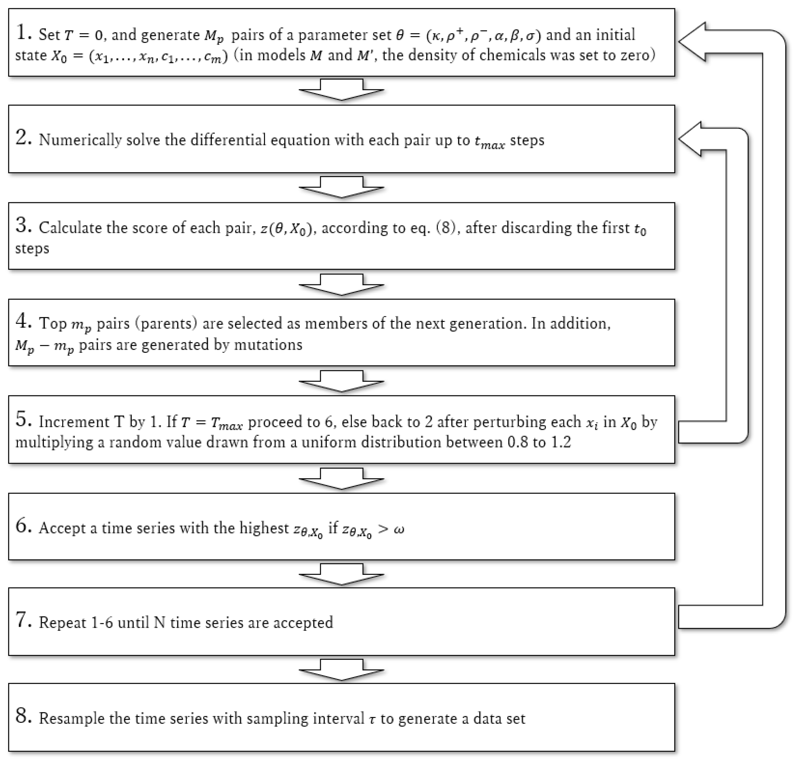
2.3. Data Preparation
2.4. Network Inference Methods
2.4.1. Pearson and Spearman Correlation Coefficient
2.4.2. Local Similarity Analysis (LSA)
2.4.3. Convergent Cross Mapping (CCM)
2.4.4. LIMITS
2.5. Evaluation
2.6. Software
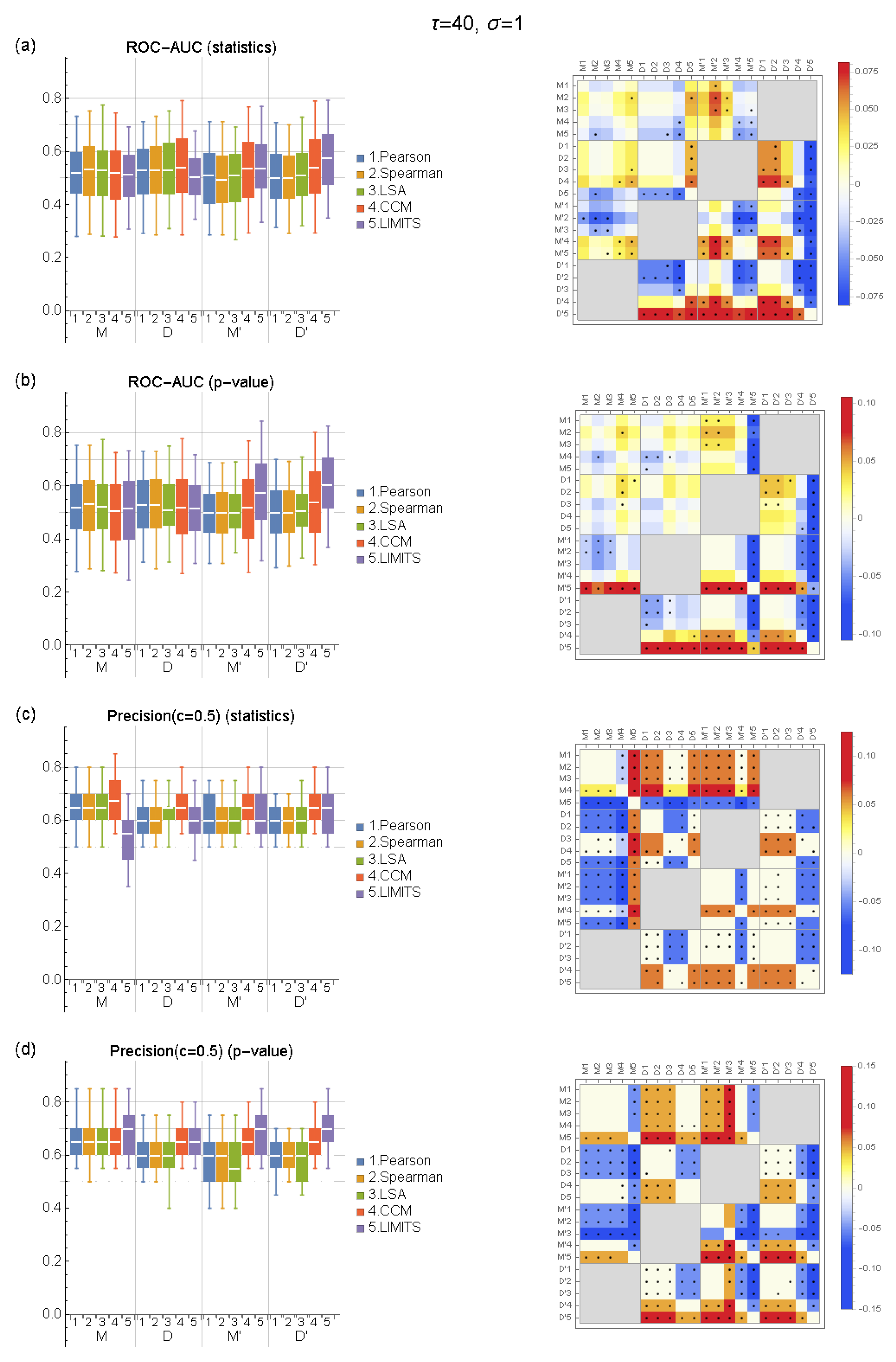
3. Results
4. Discussion
5. Conclusions
Supplementary Materials
Author Contributions
Funding
Institutional Review Board Statement
Informed Consent Statement
Data Availability Statement
Acknowledgments
Conflicts of Interest
Appendix A. Implementation of CCM for Network Inference
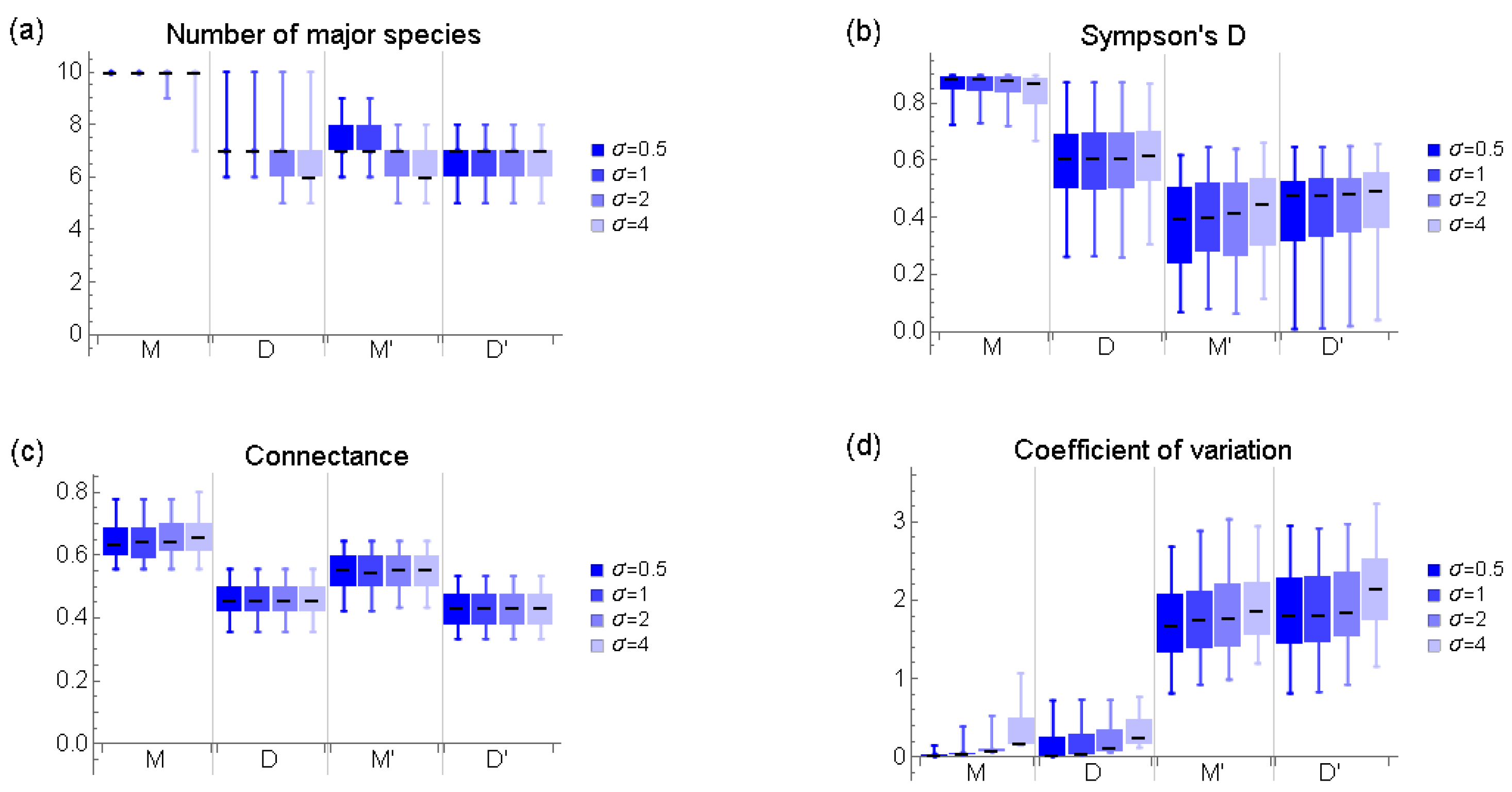
Appendix B. Basic Characteristics of Communities

References
- Lawson, C.E.; Harcombe, W.R.; Hatzenpichler, R.; Lindemann, S.R.; Löffler, F.E.; O’Malley, M.A.; Martín, H.G.; Pfleger, B.F.; Raskin, L.; Venturelli, O.S.; et al. Common principles and best practices for engineering microbiomes. Nat. Rev. Microbiol. 2019, 17, 725–741. [Google Scholar] [CrossRef] [PubMed] [Green Version]
- Layeghifard, M.; Hwang, D.M.; Guttman, D.S. Disentangling interactions in the microbiome: A network perspective. Trends Microbiol. 2017, 25, 217–228. [Google Scholar] [CrossRef] [PubMed]
- Cagua, E.F.; Wootton, K.L.; Stouffer, D.B. Keystoneness, centrality, and the structural controllability of ecological networks. J. Ecol. 2019, 107, 1779–1790. [Google Scholar] [CrossRef]
- Toju, H.; Abe, M.S.; Ishii, C.; Hori, Y.; Fujita, H.; Fukuda, S. Scoring species for synthetic community design: Network analyses of functional core microbiomes. Front. Microbiol. 2020, 11, 1361. [Google Scholar] [CrossRef] [PubMed]
- Kell, D.B.; Brown, M.; Davey, H.M.; Dunn, W.B.; Spasic, I.; Oliver, S.G. Metabolic footprinting and systems biology: The medium is the message. Nat. Rev. Microbiol. 2005, 3, 557–565. [Google Scholar] [CrossRef] [PubMed]
- D’Souza, G.; Shitut, S.; Preussger, D.; Yousif, G.; Waschina, S.; Kost, C. Ecology and evolution of metabolic cross-feeding interactions in bacteria. Nat. Prod. Rep. 2018, 35, 455–488. [Google Scholar] [CrossRef] [Green Version]
- Douglas, A.E. The microbial exometabolome: Ecological resource and architect of microbial communities. Philos. Trans. R. Soc. B 2020, 375, 20190250. [Google Scholar] [CrossRef] [Green Version]
- Pinu, F.R.; Granucci, N.; Daniell, J.; Han, T.-L.; Carneiro, S.; Rocha, I.; Nielsen, J.; Villas-Boas, S.G. Metabolite secretion in microorganisms: The theory of metabolic overflow put to the test. Metabolomics 2018, 14, 43. [Google Scholar] [CrossRef] [Green Version]
- Weiss, S.; Van Treuren, W.; Lozupone, C.; Faust, K.; Friedman, J.; Deng, Y.; Xia, L.C.; Xu, Z.Z.; Ursell, L.; Alm, E.J.; et al. Correlation detection strategies in microbial data sets vary widely in sensitivity and precision. ISME J. 2016, 10, 1669–1681. [Google Scholar] [CrossRef]
- Suzuki, K.; Yoshida, K.; Nakanishi, Y.; Fukuda, S. An equation-free method reveals the ecological interaction networks within complex microbial ecosystems. Methods Ecol. Evol. 2017, 8, 1774–1785. [Google Scholar] [CrossRef]
- Hirano, H.; Takemoto, K. Difficulty in inferring microbial community structure based on co-occurrence network approaches. BMC Bioinform. 2019, 20, 1–14. [Google Scholar] [CrossRef] [PubMed]
- Fisher, C.K.; Mehta, P. Identifying keystone species in the human gut microbiome from metagenomic timeseries using sparse linear regression. PLoS ONE 2014, 9, e102451. [Google Scholar] [CrossRef]
- Bucci, V.; Tzen, B.; Li, N.; Simmons, M.; Tanoue, T.; Bogart, E.; Deng, L.; Yeliseyev, V.; Delaney, M.L.; Liu, Q.; et al. MDSINE: Microbial Dynamical Systems INference Engine for microbiome time-series analyses. Genome Biol. 2016, 17, 1–17. [Google Scholar] [CrossRef] [Green Version]
- Alshawaqfeh, M.; Serpedin, E.; Younes, A.B. Inferring microbial interaction networks from metagenomic data using SgLV-EKF algorithm. BMC Genom. 2017, 18, 1–12. [Google Scholar] [CrossRef] [PubMed] [Green Version]
- Xiao, Y.; Angulo, M.T.; Friedman, J.; Waldor, M.K.; Weiss, S.T.; Liu, Y.Y. Mapping the ecological networks of microbial communities. Nat. Commun. 2017, 8, 1–12. [Google Scholar] [CrossRef] [PubMed] [Green Version]
- Momeni, B.; Xie, L.; Shou, W. Lotka-Volterra pairwise modeling fails to capture diverse pairwise microbial interactions. Elife 2017, 6, e25051. [Google Scholar] [CrossRef]
- Butler, S.; O’Dwyer, J.P. Stability criteria for complex microbial communities. Nat. Commun. 2018, 9, 1–10. [Google Scholar] [CrossRef] [PubMed] [Green Version]
- Brunner, J.D.; Chia, N. Metabolite-mediated modelling of microbial community dynamics captures emergent behaviour more effectively than spe-cies–species modelling. J. R. Soc. Interface 2019, 16, 20190423. [Google Scholar] [CrossRef] [PubMed] [Green Version]
- Niehaus, L.; Boland, I.; Liu, M.; Chen, K.; Fu, D.; Henckel, C.; Chaung, K.; Miranda, S.E.; Dyckman, S.; Crum, M.; et al. Microbial coexistence through chemical-mediated interactions. Nat. Commun. 2019, 10, 2052. [Google Scholar] [CrossRef] [Green Version]
- Pearson, K. Determination of the coefficient of correlation. Science 1909, 30, 23–25. [Google Scholar] [CrossRef]
- Spearman, C. The proof and measurement of association between two things. Am. J. Psychol. 1904, 15, 72–101. [Google Scholar] [CrossRef]
- Ruan, Q.; Dutta, D.; Schwalbach, M.S.; Steele, J.A.; Fuhrman, J.A.; Sun, F. Local similarity analysis reveals unique associations among marine bacterioplankton species and environmental factors. Bioinformatics 2006, 2, 2532–2538. [Google Scholar] [CrossRef] [PubMed]
- Beman, J.M.; Steele, J.A.; Fuhrman, J.A. Co-occurrence patterns for abundant marine archaeal and bacterial lineages in the deep chlorophyll maximum of coastal Cal-ifornia. ISME J. 2011, 5, 1077–1085. [Google Scholar] [CrossRef] [PubMed]
- Steele, J.A.; Countway, P.D.; Xia, L.; Vigil, P.D.; Beman, J.M.; Kim, D.Y.; Chow, C.-E.T.; Sachdeva, R.; Jones, A.C.; Schwalbach, M.S.; et al. Marine bacterial, archaeal and protistan association networks reveal ecological linkages. ISME J. 2011, 5, 1414–1425. [Google Scholar] [CrossRef] [PubMed]
- Xia, L.C.; Ai, D.; Cram, J.; Fuhrman, J.A.; Sun, F. Efficient statistical significance approximation for local similarity analysis of high-throughput time series data. Bioinformatics 2013, 29, 230–237. [Google Scholar] [CrossRef] [PubMed] [Green Version]
- Sugihara, G.; May, R.; Ye, H.; Hsieh, C.H.; Deyle, E.; Fogarty, M.; Munch, S. Detecting causality in complex ecosystems. Science 2012, 338, 496–500. [Google Scholar] [CrossRef]
- Takens, F. Detecting strange attractors in turbulence. In Dynamical Systems and Turbulence; Warwick 1980; Springer: Berlin/Heidelberg, Germany, 1981; pp. 366–381. [Google Scholar]
- Kirchman, D.L. Processes in Microbial Ecology; Oxford University Press: Oxford, UK, 2018. [Google Scholar]
- Runge, J.; Bathiany, S.; Bollt, E.; Camps-Valls, G.; Coumou, D.; Deyle, E.; Glymour, C.; Kretschmer, M.; Mahecha, M.D.; Muñoz-Marí, J.; et al. Inferring causation from time series in Earth system sciences. Nat. Commun. 2019, 10, 1–13. [Google Scholar] [CrossRef] [PubMed]
- Cao, L. Practical method for determining the minimum embedding dimension of a scalar time series. Phys. D Nonlinear Phenom. 1997, 110, 43–50. [Google Scholar] [CrossRef]
- May, R.M. Stability and Complexity in Model Ecosystems; Princeton University Press: Princeton, NJ, USA, 1973. [Google Scholar]


| Description | Value | |
|---|---|---|
| n | Number of microbes | 10 |
| m | Number of chemicals | 5 |
| Carrying capacity | 1 | |
| Dilution rate | 0.01 | |
| Growth rate | ||
| Half-saturation density | ||
| Positive effect of chemicals on microbes | ||
| Negative effect of chemicals on microbes | ||
| Maximum consumption rate of chemicals | ||
| Production rate of chemicals | ||
| Influx of microbes |
| Name | Description | Value |
|---|---|---|
| N | Number of time series in a data set | 288 |
| Number of pairs in each generation | 32 | |
| Number of parents for next generation | 4 | |
| Length of time series generated by simulation | 10,000 | |
| Length of time series discarded as the initial transient | ||
| Number of iterations of the optimization procedure | 60 (for M and D) 120 (for M′ and D′) | |
| Criterion for major species | ||
| Threshold value for the evaluation function | 5 |
Publisher’s Note: MDPI stays neutral with regard to jurisdictional claims in published maps and institutional affiliations. |
© 2022 by the authors. Licensee MDPI, Basel, Switzerland. This article is an open access article distributed under the terms and conditions of the Creative Commons Attribution (CC BY) license (https://creativecommons.org/licenses/by/4.0/).
Share and Cite
Suzuki, K.; Abe, M.S.; Kumakura, D.; Nakaoka, S.; Fujiwara, F.; Miyamoto, H.; Nakaguma, T.; Okada, M.; Sakurai, K.; Shimizu, S.; et al. Chemical-Mediated Microbial Interactions Can Reduce the Effectiveness of Time-Series-Based Inference of Ecological Interaction Networks. Int. J. Environ. Res. Public Health 2022, 19, 1228. https://doi.org/10.3390/ijerph19031228
Suzuki K, Abe MS, Kumakura D, Nakaoka S, Fujiwara F, Miyamoto H, Nakaguma T, Okada M, Sakurai K, Shimizu S, et al. Chemical-Mediated Microbial Interactions Can Reduce the Effectiveness of Time-Series-Based Inference of Ecological Interaction Networks. International Journal of Environmental Research and Public Health. 2022; 19(3):1228. https://doi.org/10.3390/ijerph19031228
Chicago/Turabian StyleSuzuki, Kenta, Masato S. Abe, Daiki Kumakura, Shinji Nakaoka, Fuki Fujiwara, Hirokuni Miyamoto, Teruno Nakaguma, Mashiro Okada, Kengo Sakurai, Shohei Shimizu, and et al. 2022. "Chemical-Mediated Microbial Interactions Can Reduce the Effectiveness of Time-Series-Based Inference of Ecological Interaction Networks" International Journal of Environmental Research and Public Health 19, no. 3: 1228. https://doi.org/10.3390/ijerph19031228