Productivity Effect Evaluation on Market-Type Environmental Regulation: A Case Study of SO2 Emission Trading Pilot in China


Abstract
:1. Introduction
2. Policy Background and Research Hypothesis
2.1. Policy Background
2.2. Research Hypothesis
3. Empirical Strategy
3.1. Empirical Model
3.2. Sample and Data
3.3. Measurement of Main Variable TFP
3.4. Other Variables
4. Results
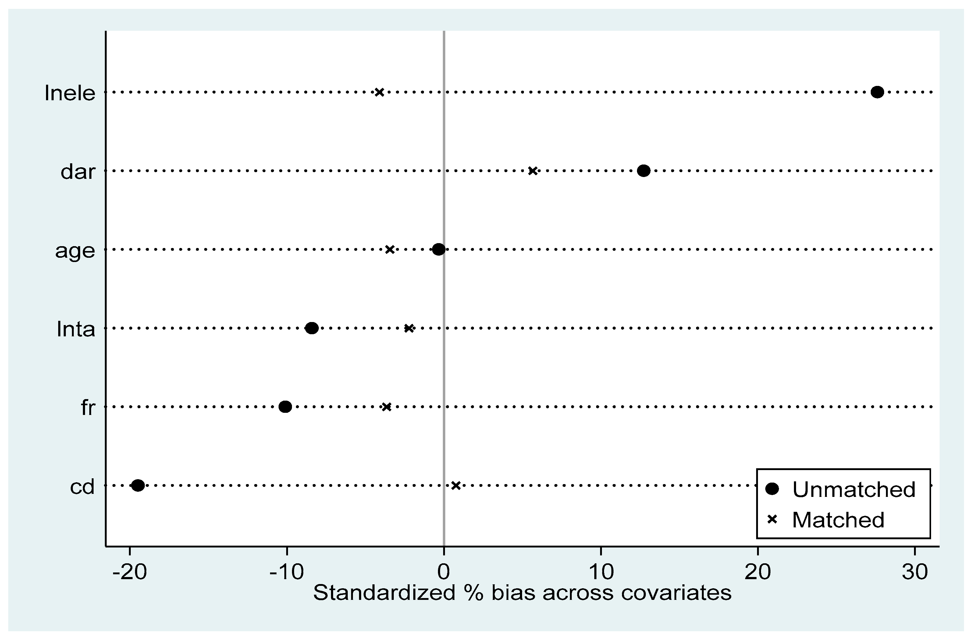
4.1. Result of PSM
4.2. Baseline Estimations
4.3. Robustness Tests
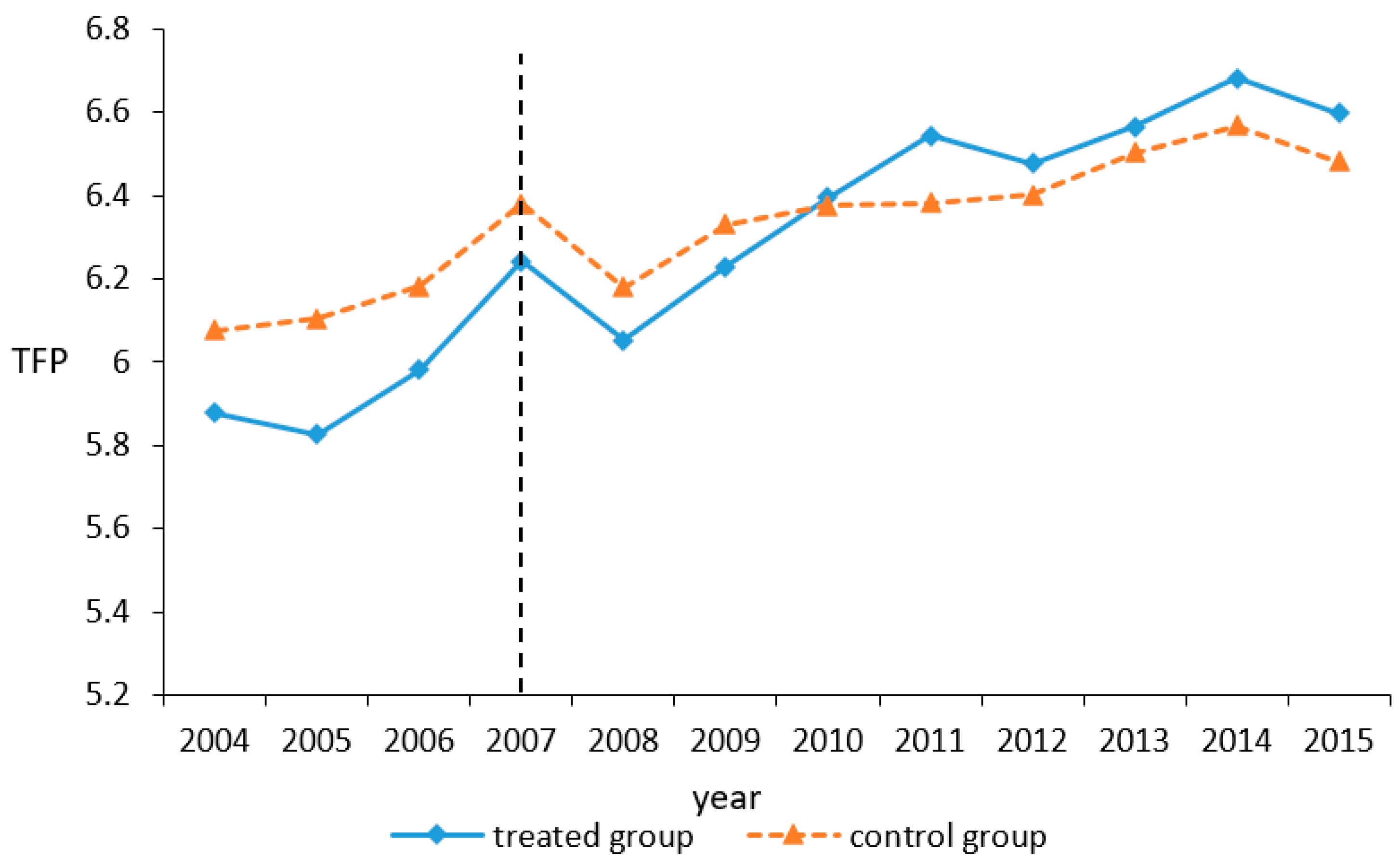
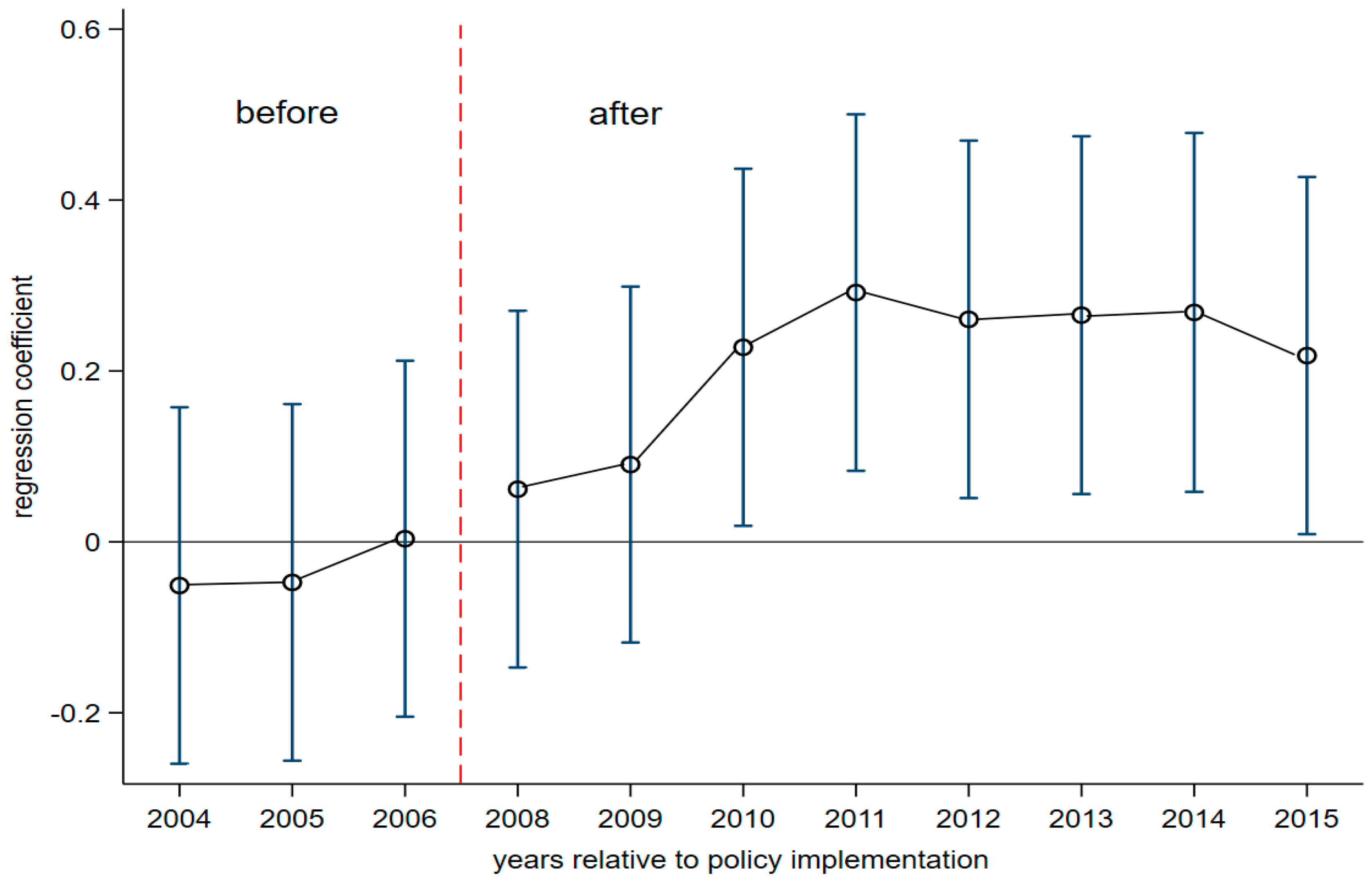
4.3.1. Parallel Trend Test
4.3.2. Alternative Variable Test
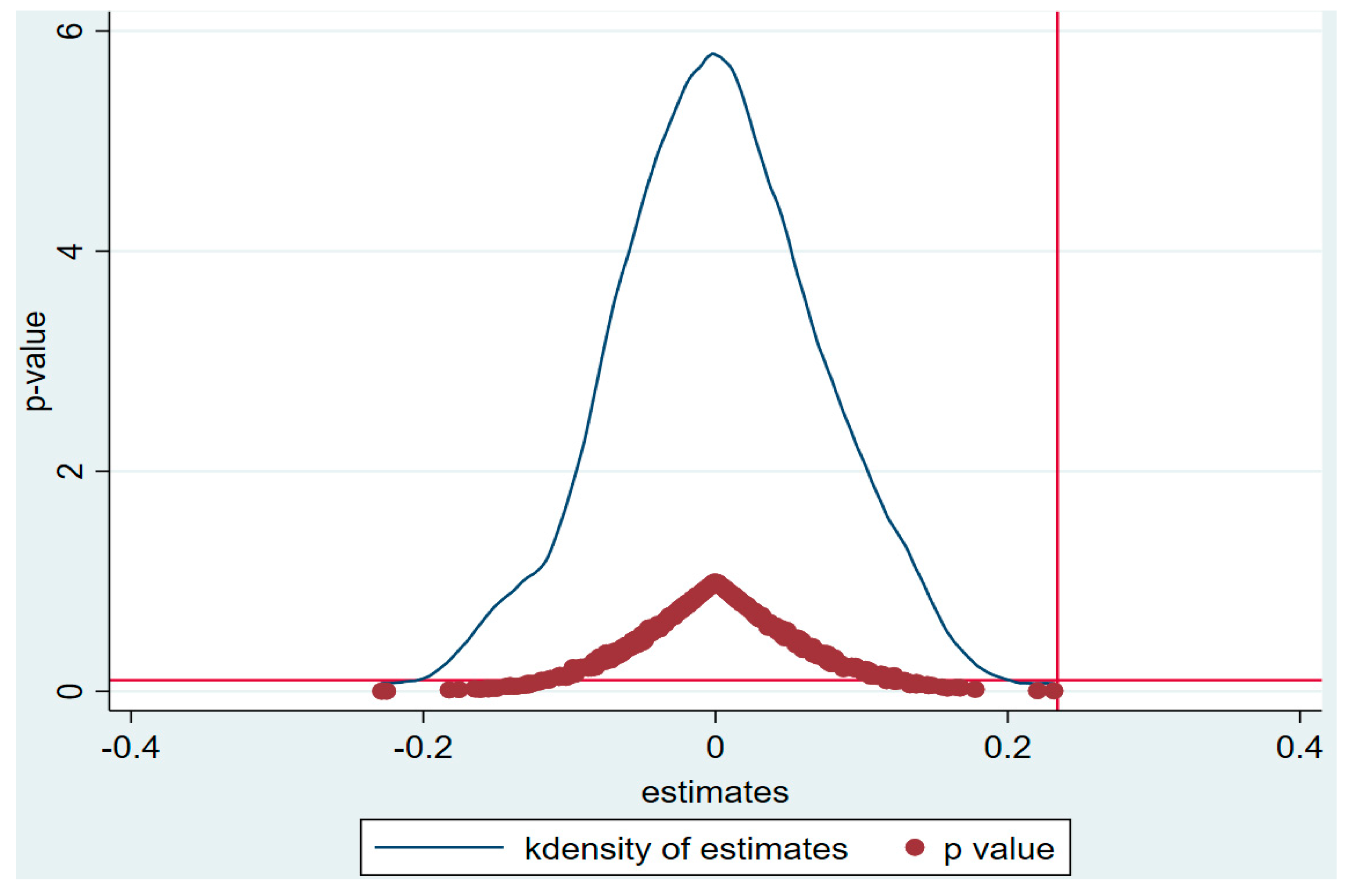
4.3.3. Placebo Test
4.3.4. DDD Test
5. Heterogeneity and Moderating Effects Analysis
5.1. Heterogeneity Analysis
5.2. Moderating Effects Analysis
5.2.1. Moderating Effect of Financing Constraint
5.2.2. Moderating Effect of Bargaining Power
6. Conclusions
Author Contributions
Funding
Acknowledgments
Conflicts of Interest
Appendix A

| Variable | Unmatched | Mean | %Reduct | t-Test | V(T)/V(C) | |||
|---|---|---|---|---|---|---|---|---|
| Matched | Treated | Control | %bias | |bias| | t | p > |t| | ||
| cd | U | 0.76 | 1.03 | −19.5 | −5.09 | 0.00 | 0.45 * | |
| M | 0.76 | 0.75 | 0.8 | 96.1 | 0.25 | 0.81 | 1.16 * | |
| lnta | U | 8.32 | 8.43 | −8.4 | −2.27 | 0.02 | 0.82 * | |
| M | 8.32 | 8.35 | −2.2 | 73.5 | −0.56 | 0.58 | 0.87 * | |
| fr | U | 0.37 | 0.39 | −10.1 | −2.74 | 0.01 | 0.91 | |
| M | 0.37 | 0.38 | −3.7 | 63.7 | −0.92 | 0.36 | 0.98 | |
| age | U | 15.63 | 15.65 | −0.3 | −0.09 | 0.93 | 1.88 * | |
| M | 15.63 | 15.86 | −3.5 | −931.8 | −0.85 | 0.40 | 1.83 * | |
| dar | U | 0.57 | 0.55 | 12.7 | 3.41 | 0.00 | 0.74 * | |
| M | 0.57 | 0.56 | 5.6 | 55.6 | 1.41 | 0.16 | 0.78 * | |
| lnele | U | 8.06 | 7.74 | 27.6 | 7.21 | 0.00 | 0.44 * | |
| M | 8.06 | 8.10 | −4.1 | 85.1 | −1.12 | 0.26 | 0.60 * | |

References
- Hao, J.; He, H.; Duan, L.; Li, J.; Wang, L. Air pollution and its control in China. Front. Environ. Sci. Eng. China 2007, 1, 129–142. [Google Scholar] [CrossRef]
- Zeng, Y.Y.; Cao, Y.F.; Qiao, X.; Seyler, B.C.; Tang, Y. Air pollution reduction in China: Recent success but great challenge for the future. Sci. Total Environ. 2019, 663, 329–337. [Google Scholar] [CrossRef] [PubMed]
- Hering, L.; Poncet, S. Environmental policy and exports: Evidence from Chinese cities. J. Environ. Econ. Manag. 2014, 68, 296–318. [Google Scholar] [CrossRef]
- He, J. What is the role of openness for China’s aggregate industrial SO2 emission?: A structural analysis based on the Divisia decomposition method. Ecol. Econ. 2010, 69, 868–886. [Google Scholar] [CrossRef]
- Peng, J.; Xie, R.; Ma, C.; Fu, Y. Market-based environmental regulation and total factor productivity: Evidence from Chinese enterprises. Econ. Model. 2020. [Google Scholar] [CrossRef]
- Martin, R.; Muûls, M.; Wagner, U. The Impact of the European Union Emissions Trading Scheme on Regulated Firms: What Is the Evidence after Ten Years? Rev. Environ. Econ. Policy 2015, 10, rev016. [Google Scholar] [CrossRef] [Green Version]
- Oestreich, A.M.; Tsiakas, I. Carbon emissions and stock returns: Evidence from the EU Emissions Trading Scheme. J. Bank Financ. 2015, 58, 294–308. [Google Scholar] [CrossRef]
- Tang, H.-L.; Liu, J.-M.; Mao, J.; Wu, J.-G. The effects of emission trading system on corporate innovation and productivity-empirical evidence from China’s SO2 emission trading system. Environ. Sci. Pollut. Res. 2020, 27. [Google Scholar] [CrossRef]
- Porter, M. America’s Green Strategy. Sci. Am. 1991, 264. [Google Scholar] [CrossRef]
- Porter, M.E.; Van der Linde, C. Toward a New Conception of the Environment-Competitiveness Relationship. J. Econ. Perspect. 1995, 9, 97–118. [Google Scholar] [CrossRef]
- Schleich, J.; Betz, R. EU emissions trading and transaction costs for small and medium sized companies. Interecon. Rev. Eur. Econ. Policy 2004, 39, 121–123. [Google Scholar] [CrossRef]
- Testa, F.; Iraldo, F.; Frey, M. The effect of environmental regulation on firms’ competitive performance: The case of the building & construction sector in some EU regions. J. Environ. Manag. 2011, 92, 2136–2144. [Google Scholar] [CrossRef]
- Rubashkina, Y.; Galeotti, M.; Verdolini, E. Environmental Regulation and Competitiveness: Empirical Evidence on the Porter Hypothesis from European Manufacturing Sectors. SSRN Electron. J. 2014, 83. [Google Scholar] [CrossRef]
- Calel, R.; Dechezleprêtre, A. Environmental Policy and Directed Technological Change: Evidence from the European Carbon Market. Rev. Econ. Stat. 2012, 98. [Google Scholar] [CrossRef]
- Albrizio, S.; Kozluk, T.; Zipperer, V. Environmental policies and productivity growth: Evidence across industries and firms. J. Environ. Econ. Manag. 2017, 81, 209–226. [Google Scholar] [CrossRef]
- Chintrakarn, P. Environmental regulation and U.S. states’ technical inefficiency. Econ. Lett. 2008, 100, 363–365. [Google Scholar] [CrossRef]
- Liu, Z.; Mao, X.; Tu, J.; Jaccard, M. A comparative assessment of economic-incentive and command-and-control instruments for air pollution and CO2 control in China’s iron and steel sector. J. Environ. Manag. 2014, 144C, 135–142. [Google Scholar] [CrossRef]
- Gray, W.; Shadbegian, R. Plant Vintage, Technology, and Environmental Regulation. J. Environ. Econ. Manag. 2003, 46, 384–402. [Google Scholar] [CrossRef] [Green Version]
- Lanoie, P.; Patry, M.; Lajeunesse, R. Environmental Regulation and Productivity: Testing the Porter Hypothesis. J. Product. Anal. 2008, 30, 121–128. [Google Scholar] [CrossRef]
- Greenstone, M.; List, J.A.; Syverson, C. The Effects of Environmental Regulation on the competitiveness of US Manufacturing. NBER Work. Pap. 2012, 18392. [Google Scholar] [CrossRef]
- Kozluk, T.; Zipperer, V. Environmental policies and productivity growth. OECD J. Econ. Stud. 2014, 2014. [Google Scholar] [CrossRef] [Green Version]
- Cohen, M.; Tubb, A. The Impact of Environmental Regulation on Firm and Country Competitiveness: A Meta-Analysis of the Porter Hypothesis. SSRN Electron. J. 2015. [Google Scholar] [CrossRef] [Green Version]
- Li, B.; Wu, S. Effects of local and civil environmental regulation on green total factor productivity in China: A spatial Durbin econometric analysis. J. Clean. Prod. 2016, 153. [Google Scholar] [CrossRef]
- Hua, Y.; Xie, R.; Su, Y. Fiscal Spending and Air Pollution in Chinese Cities: Identifying Composition and Technique Effects. China Econ. Rev. 2017. [Google Scholar] [CrossRef]
- Dechezlepretre, A.; Sato, M. The Impacts of Environmental Regulations on Competitiveness. Rev. Environ. Econ. Policy 2017, 11, 183–206. [Google Scholar] [CrossRef] [Green Version]
- Liu, X.; Lin, B.; Zhang, Y. Sulfur Dioxide Emission Reduction of Power Plants in China: Current Policies and Implications. J. Clean. Prod. 2015, 113. [Google Scholar] [CrossRef]
- Carrion Flores, C.; Innes, R. Environmental Innovation and environmental performance. J. Environ. Econ. Manag. 2010, 59, 27–42. [Google Scholar] [CrossRef]
- Zhao, X.; Sun, B. The influence of Chinese environmental regulation on corporation innovation and competitiveness. J. Clean. Prod. 2015. [Google Scholar] [CrossRef]
- Davies, G.; Kendall, G.; Soane, E.; Li, J.; Rocks, S.; Jude, S.; Pollard, S. Regulators as agents: Modelling personality and power as evidence is brokered to support decisions on environmental risk. Sci. Total Environ. 2013, 466, 74–83. [Google Scholar] [CrossRef] [Green Version]
- Chen, Y.; Li, P.; Lu, Y. Career concerns and multitasking local bureaucrats: Evidence of a target-based performance evaluation system in China. J. Dev. Econ. 2018, 133. [Google Scholar] [CrossRef]
- Hamamoto, M. Environmental Regulation and the Productivity of Japanese Manufacturing Industries. Resour. Energy Econ. 2006, 28, 299–312. [Google Scholar] [CrossRef]
- Anderson, B.; Convery, F.; Di Maria, C. Technological Change and the EU ETS: The Case of Ireland. SSRN Electron. J. 2011. [Google Scholar] [CrossRef]
- Hoffmann, V. EU ETS and Investment Decisions: The Case of the German Electricity Industry. Eur. Manag. J. 2007, 25, 464–474. [Google Scholar] [CrossRef]
- Borghesi, S.; Cainelli, G.; Mazzanti, M. Linking emission trading to environmental innovation: Evidence from the Italian manufacturing industry. Res. Policy 2014, 44. [Google Scholar] [CrossRef]
- Jiang, J.; Xie, D.; Bin, Y.; Shen, B.; Chen, Z.-M. Research on China’s cap-and-trade carbon emission trading scheme: Overview and outlook. Appl. Energy 2016, 178. [Google Scholar] [CrossRef]
- Levinson, A.; Taylor, M.S. Unmasking the Pollution Haven Effect. Int. Econ. Rev. 2008, 49, 223–254. [Google Scholar] [CrossRef] [Green Version]
- Firpo, S.; Fortin, N.M.; Lemieux, T. Unconditional Quantile Regressions. Econometrica 2009, 77, 953–973. [Google Scholar] [CrossRef] [Green Version]
- Borgen, N. Fixed Effects in Unconditional Quantile Regression. Stata J. Promot. Commun. Stat. Stata 2016, 16, 403–415. [Google Scholar] [CrossRef] [Green Version]
- Imbens, G.W.; Wooldridge, J.M. Recent Developments in the Econometrics of Program Evaluation. J. Econ. Lit. 2009, 47, 5–86. [Google Scholar] [CrossRef] [Green Version]
- Baum-Snow, N.; Ferreira, F. Causal Inference in Urban and Regional Economics. Handb. Reg. Urban Econ. 2015, 5, 3–68. [Google Scholar] [CrossRef]
- Guariglia, A.; Liu, P. To what extent do financing constraints affect Chinese firms’ innovation activities? Int. Rev. Financ. Anal. 2014, 36, 223–240. [Google Scholar] [CrossRef]
- Madrid-Guijarro, A.; Garcia-Perez-de-Lema, D.; Van Auken, H. Financing constraints and SME innovation during economic crises. Acad. Rev. Latinoam. Adm. 2016, 29, 84–106. [Google Scholar] [CrossRef]
- Li, H.; Zhou, L.-A. Political Turnover and Economic Performance: The Incentive Role of Personnel Control in China. J. Public Econ. 2005, 89, 1743–1762. [Google Scholar] [CrossRef]
- Li, P.; Chen, Y. The Influence of Enterprises’ Bargaining Power on the Green Total Factor Productivity Effect of Environmental Regulation—Evidence from China. Sustainability 2019, 11, 4910. [Google Scholar] [CrossRef] [Green Version]
- Heckman, J.J.; Ichimura, H.; Todd, P.E. Matching as an Econometric Evaluation Estimator: Evidence from Evaluating a Job Training Programme. Rev. Econ. Stud. 1997, 64, 605–654. [Google Scholar] [CrossRef]
- Heckman, J.; Ichimura, H.; Smith, J.; Todd, P. Characterizing selection bias using experimental data. Econometrica 1998, 66, 1017–1098. [Google Scholar] [CrossRef]
- Mollisi, V.; Rovigatti, G. Theory and Practice of TFP Estimation: The Control Function Approach Using Stata. SSRN Electron. J. 2017. [Google Scholar] [CrossRef]
- Zucker, T.; Flesche, C.W.; Germing, U.; Schroter, S.; Willers, R.; Wolf, H.-H.; Heyll, A.; Blundell, R.; Bond, S. Initial conditions and moment restrictions in dynamic panel data models—Monte Carlo evidence and an application to employment equations. J. Econom. 1998, 87, 115–143. [Google Scholar]
- Wooldridge, J.M. On estimating firm-level production functions using proxy variables to control for unobservables. Econ. Lett. 2009, 104, 112–114. [Google Scholar] [CrossRef]
- Brandt, L.; Biesebroeck, J.; Zhang, Y. Creative Accounting or Creative Destruction? Firm-Level Productivity Growth in Chinese Manufacturing. J. Dev. Econ. 2009, 97, 339–351. [Google Scholar] [CrossRef] [Green Version]
- Klenow, P.; Hsieh, C.-T. Misallocation and Manufacturing TFP in China and India. Q. J. Econ. 2009, 124, 1403–1448. [Google Scholar] [CrossRef] [Green Version]
- Porter, M.; Linde, C. Green and Competitive: Ending the Stalemate. Long Range Plan. 1995, 28. [Google Scholar] [CrossRef]
- Ambec, S.; Cohen, M.; Elgie, S.; Lanoie, P. The Porter Hypothesis at 20: Can Environmental Regulation Enhance Innovation and Competitiveness? Ciranocirano Work. Pap. 2010, 7. [Google Scholar] [CrossRef] [Green Version]
- Montgomery, W. Markets in Licenses and Efficient Pollution Control Programs. J. Econ. Theory 1972, 5, 395–418. [Google Scholar] [CrossRef]
- Prato, T. Natural Resource and Environmental Economics; Iowa State University Press: Ames, IA, USA, 1998. [Google Scholar]
- Li, Z.; Liao, G.; Albitar, K. Does corporate environmental responsibility engagement affect firm value? The mediating role of corporate innovation. Bus. Strategy Environ. 2019. [Google Scholar] [CrossRef]
- Parry, I.; Goulder, L. Instrument Choice in Environmental Policy. Rev. Environ. Econ. Policy 2008, 2. [Google Scholar] [CrossRef] [Green Version]
- Bloom, N.; Bloom, D.; Reenen, J. Measuring and Explaining Management Practices across Firms and Countries. Q. J. Econ. 2007, 122, 1351–1408. [Google Scholar] [CrossRef]
- Comin, D.; Hobijn, B. An Exploration of Technology Diffusion. Am. Econ. Rev. 2010, 100, 2031–2059. [Google Scholar] [CrossRef] [Green Version]
- Ferrando, A.; Ruggieri, A. Financial constraints and productivity: Evidence from euro area companies. Int. J. Financ. Econ. 2018, 23, 257–282. [Google Scholar] [CrossRef]
- Benito, A.; Hernando, I. Firm behaviour and financial pressure: Evidence from Spanish panel data. Bull. Econ. Res. 2007, 59, 283–311. [Google Scholar] [CrossRef]
- Aghion, P.; Dechezleprêtre, A.; Hemous, D.; Martin, R.; Reenen, J. Carbon Taxes, Path Dependency and Directed Technical Change: Evidence from the Auto Industry. J. Polit. Econ. 2012, 124. [Google Scholar] [CrossRef] [Green Version]
- Managi, S.; Kaneko, S. Environmental Productivity in China. Econ. Bull. 2004, 17, 1–10. [Google Scholar]
- Abadie, A.; Imbens, G.; Drukker, D.; Herr, J. Implementing Matching Estimators for Average Treatment Effects in STATA. Stata J. 2004, 4, 290–311. [Google Scholar] [CrossRef] [Green Version]
- Lu, J.H. The Performance of Performance-Based Contracting in Human Services: A Quasi-Experiment. J. Public Adm. Res. Theory 2016, 26, 277–293. [Google Scholar] [CrossRef] [Green Version]
- Olley, G.S.; Pakes, A. The Dynamics of Productivity in the Telecommunications Equipment Industry. Econometrica 1996, 64, 1263–1297. [Google Scholar] [CrossRef]
- Levinsohn, J.; Petrin, A. Estimating Production Functions Using Inputs to Control for Unobservables. Rev. Econ. Stud. 2003, 70, 317–341. [Google Scholar] [CrossRef]
- Schumpeter, J.A.; Schumpeter, J.; Schumpeter, J. The theory of economics development. J. Polit. Econ. 1934, 1, 170–172. [Google Scholar] [CrossRef]
- Cole, M.; Elliott, R.; Toshihiro, O. Trade, Environmental Regulations and Industrial Mobility: An Industry-level Study of Japan. Ecol. Econ. 2010, 69, 1995–2002. [Google Scholar] [CrossRef] [Green Version]
- Yu, M. Processing Trade, Tarff Reductions, and Firm Productivity: Evidence from Chinese Firms. Econ. J. 2011, 125. [Google Scholar] [CrossRef]
- Haque, A.; Fatima, H.; Abid, A.; Qamar, M. Impact of firm-level uncertainty on earnings management and role of accounting conservatism. Quant. Financ. Econ. 2019, 3, 772–794. [Google Scholar] [CrossRef]
- Sean, C. The Relationship between Firm Investment and Financial Status. J. Financ. 1999. [Google Scholar] [CrossRef]
- Lamont, O.; Polk, C.; Saa-Requejo, J. Financial Constraints and Stock Returns. Rev. Financ. Stud. 2001, 14, 529–554. [Google Scholar] [CrossRef]
- Whited, T.M.; Wu, G. Financial Constraints Risk. Rev. Financ. Stud. 2006, 19, 531–559. [Google Scholar] [CrossRef]
- Hadlock, C.J.; Pierce, J.R. New Evidence on Measuring Financial Constraints: Moving Beyond the KZ Index. Rev. Financ. Stud. 2010, 23, 1909–1940. [Google Scholar] [CrossRef]
- Alder, S.; Shao, L.; Zilibotti, F. Economic reforms and industrial policy in a panel of Chinese cities. J. Econ. Growth 2016, 21, 305–349. [Google Scholar] [CrossRef]
- Beck, T.; Levine, R.; Levkov, A. Big bad banks? The winners and losers from bank deregulation in the United States. J. Financ. 2010, 65, 1637–1667. [Google Scholar] [CrossRef] [Green Version]
- Cai, X.; Lu, Y.; Wu, M.; Yu, L. Does Environmental Regulation Drive away Inbound Foreign Direct Investment? Evidence from a Quasi-Natural Experiment in China. J. Dev. Econ. 2016, 123. [Google Scholar] [CrossRef]
- Li, Z.; Dong, H.; Huang, Z.; Failler, P. Impact of Foreign Direct Investment on Environmental Performance. Sustainability 2019, 11, 3538. [Google Scholar] [CrossRef] [Green Version]
- Broni, M.; Hosen, M.; Masih, M. Does a country’s external debt level affect its Islamic banking sector development? Evidence from Malaysia based on Quantile regression and Markov regime-switching. Quant. Financ. Econ. 2019, 3, 366–389. [Google Scholar] [CrossRef]
- Kanamura, T. Supply-Side Perspective for Carbon Pricing. Quant. Financ. Econ. 2019, 3, 109–123. [Google Scholar] [CrossRef]
- Li, Z.; Liao, G.; Wang, Z.; Huang, Z. Green loan and subsidy for promoting clean production innovation. J. Clean. Prod. 2018, 187. [Google Scholar] [CrossRef]


| Variable | Obs | Mean | Std. Dev. | Min | Max |
|---|---|---|---|---|---|
| TFP | 3120 | 6.327 | 0.922 | 3.046 | 8.539 |
| TFP(LP) | 3120 | 4.850 | 0.875 | 1.680 | 7.072 |
| cd | 3120 | 0.927 | 1.485 | 0.025 | 8.294 |
| fr | 3120 | 0.381 | 0.187 | 0.023 | 0.782 |
| lnta | 3120 | 8.386 | 1.292 | 5.198 | 11.451 |
| age | 3120 | 15.642 | 6.409 | 3 | 73 |
| owner | 3120 | 0.596 | 0.491 | 0 | 1 |
| roa | 3120 | 0.025 | 0.064 | −0.279 | 0.197 |
| dar | 3120 | 0.555 | 0.208 | 0.107 | 1.424 |
| lnele | 3120 | 7.866 | 1.192 | 4.094 | 10.068 |
| fc | 3120 | 3.710 | 0.261 | 2.949 | 5.721 |
| bar | 3120 | 17.052 | 1.454 | 11.721 | 21.409 |
| TFP | (1) | (2) | (3) | (4) |
|---|---|---|---|---|
| time*treated | 0.235 *** | 0.223 *** | 0.234 *** | 0.234 *** |
| (3.73) | (4.51) | (4.64) | (5.05) | |
| cd | 0.047 *** | 0.042 ** | ||
| (3.94) | (2.41) | |||
| lnta | 0.340 *** | 0.179 *** | ||
| (26.69) | (7.61) | |||
| fr | −0.989 *** | −0.910 *** | ||
| (−11.65) | (−7.70) | |||
| age | −0.001 | 0.023 *** | ||
| (−0.23) | (3.98) | |||
| owner | 0.029 | |||
| (1.03) | ||||
| roa | 4.671 *** | 3.679 *** | ||
| (21.45) | (16.34) | |||
| dar | −0.378 *** | −0.322 *** | ||
| (−5.21) | (−3.37) | |||
| lnele | 0.063 *** | 0.069 *** | ||
| (2.86) | (3.34) | |||
| _cons | 6.306 *** | 3.420 *** | 6.016 *** | 4.223 *** |
| (32.97) | (14.72) | (149.81) | (17.94) | |
| industry fe | yes | yes | yes | yes |
| area fe | yes | yes | yes | yes |
| year fe | yes | yes | yes | yes |
| individual fe | no | no | yes | yes |
| observations | 3099 | 3099 | 3099 | 3099 |
| R-squared | 0.243 | 0.544 | 0.039 | 0.423 |
| TFP | (1) | (2) |
|---|---|---|
| treated * year2004 | −0.072 (−0.62) | −0.051 (−0.48) |
| treated * year2005 | −0.098 (−0.84) | −0.047 (−0.45) |
| treated * year2006 | −0.037 (−0.32) | 0.004 (0.04) |
| treated * year2007 | omitted | omitted |
| treated * year2008 | 0.035 (0.30) | 0.062 (0.58) |
| treated * year2009 | 0.048 (0.41) | 0.090 (0.85) |
| treated * year2010 | 0.166 (1.43) | 0.228 ** (2.14) |
| treated * year2011 | 0.273 ** (2.34) | 0.292 *** (2.74) |
| treated * year2012 | 0.226 * (1.94) | 0.260 ** (2.44) |
| treated * year2013 | 0.216 * (1.86) | 0.265 ** (2.49) |
| treated * year2014 | 0258 ** (2.22) | 0.269 ** (2.51) |
| treated * year2015 | 0.236 ** (2.03) | 0.218 ** (2.05) |
| Constant | 6.045 *** (99.58) | 4.258 (17.24) |
| Control variables | no | added |
| industry fe | yes | yes |
| area fe | yes | yes |
| year fe | yes | yes |
| individual fe | yes | yes |
| observations | 3099 | 3099 |
| R-squared | 0.100 | 0.253 |
| TFP | (1) | (2) | (3) | (4) |
|---|---|---|---|---|
| time*treated | 0.244 *** | 0.235 *** | 0.243 *** | 0.245 *** |
| (4.02) | (4.75) | (4.83) | (5.29) | |
| cd | 0.092 *** | 0.082 *** | ||
| (7.66) | (4.74) | |||
| lnta | 0.217 *** | 0.070 *** | ||
| (17.02) | (2.96) | |||
| fr | −1.258 *** | −1.161 *** | ||
| (−14.79) | (−9.82) | |||
| age | −0.001 | 0.024 *** | ||
| (−0.63) | (4.14) | |||
| owner | 0.025 | omitted | ||
| (0.87) | ||||
| roa | 4.665 *** | 3.662 *** | ||
| (21.39) | (16.26) | |||
| dar | −0.389 *** | −0.326 *** | ||
| (−5.34) | (−3.41) | |||
| lnele | 0.053 ** | 0.059 *** | ||
| (2.39) | (2.86) | |||
| _cons | 4.887 *** | 3.152 *** | 4.598 *** | 3.785 *** |
| (26.57) | (13.54) | (114.65) | (16.07) | |
| industry fe | yes | yes | yes | yes |
| area fe | yes | yes | yes | yes |
| year fe | yes | yes | yes | yes |
| individual fe | no | no | yes | yes |
| observations | 3099 | 3099 | 3099 | 3099 |
| R-squared | 0.223 | 0.492 | 0.028 | 0.352 |
| TFP | (1) | (2) | (3) | (4) |
|---|---|---|---|---|
| time*treated*polluting | 0.078 | 0.194 *** | 0.389 *** | 0.358 *** |
| (0.90) | (2.97) | (5.36) | (5.45) | |
| time*treated | −0.001 | −0.060 | −0.155 *** | −0.137 *** |
| (−0.02) | (−1.23) | (−3.00) | (−2.93) | |
| time*polluting | −0.097 ** | −0.147 *** | −0.408 *** | −0.316 *** |
| (−2.17) | (−4.30) | (−9.06) | (−7.70) | |
| treated*polluting | 0.097 | −0.092 * | 0.000 | 0.000 |
| (1.43) | (−1.79) | (.) | (.) | |
| cd | 0.044 *** | 0.032 ** | ||
| (4.08) | (2.13) | |||
| lnta | 0.360 *** | 0.253 *** | ||
| (41.97) | (15.37) | |||
| fr | −1.270 *** | −1.186 *** | ||
| (−19.54) | (−12.89) | |||
| age | −0.001 | 0.043 *** | ||
| (−0.29) | (9.63) | |||
| owner | 0.018 | 0.000 | ||
| (0.94) | (.) | |||
| roa | 4.597 *** | 3.444 *** | ||
| (31.40) | (22.78) | |||
| dar | −0.156 *** | −0.198 *** | ||
| (−3.34) | (−3.06) | |||
| lnele | 0.035 ** | 0.037 ** | ||
| (2.16) | (2.49) | |||
| _cons | 5.860 *** | 3.461 *** | 5.962 *** | 3.731 *** |
| (34.04) | (19.25) | (206.96) | (22.64) | |
| industry fe | yes | yes | yes | yes |
| area fe | yes | yes | yes | yes |
| year fe | yes | yes | yes | yes |
| individual fe | no | yes | no | yes |
| observations | 6183 | 6183 | 6183 | 6183 |
| R-squared | 0.187 | 0.538 | 0.072 | 0.425 |
| TFP | (1) | (2) | (3) | (4) | (5) | (6) | (7) | (8) | (9) |
|---|---|---|---|---|---|---|---|---|---|
| 10th | 20th | 30th | 40th | 50th | 60th | 70th | 80th | 90th | |
| time*treated | 0.190 | 0.125 | 0.142 | 0.238 ** | 0.254 *** | 0.256 *** | 0.264 *** | 0.195 ** | 0.095 |
| (0.88) | (0.96) | (1.36) | (2.44) | (2.77) | (3.04) | (2.91) | (1.99) | (0.77) | |
| cd | 0.018 | 0.012 | 0.046 | 0.013 | 0.015 | 0.033 | 0.052 | 0.073 | 0.095 |
| (0.33) | (0.34) | (1.29) | (0.39) | (0.49) | (0.86) | (1.50) | (1.58) | (1.43) | |
| lnta | 0.274 * | 0.173 ** | 0.137 ** | 0.158 *** | 0.176 *** | 0.181 *** | 0.095 ** | 0.090 * | 0.031 |
| (1.93) | (2.36) | (2.33) | (2.91) | (3.50) | (3.78) | (1.98) | (1.87) | (0.45) | |
| fr | −1.290 ** | −1.030 *** | −1.093 *** | −1.005 *** | −0.891 *** | −0.914 *** | −0.804 *** | −0.809 *** | −0.832 *** |
| (−2.11) | (−3.15) | (−4.19) | (−4.00) | (−4.11) | (−4.14) | (−3.57) | (−3.34) | (−2.91) | |
| age | −0.011 | 0.031 ** | 0.046 *** | 0.046 *** | 0.039 *** | 0.028 *** | 0.040 *** | 0.037 *** | 0.048 *** |
| (−0.45) | (2.13) | (4.23) | (4.63) | (4.21) | (3.21) | (4.55) | (3.77) | (3.62) | |
| owner | 0.000 | 0.000 | 0.000 | 0.000 | 0.000 | 0.000 | 0.000 | 0.000 | 0.000 |
| (.) | (.) | (.) | (.) | (.) | (.) | (.) | (.) | (.) | |
| roa | 5.171 *** | 4.324 *** | 3.258 *** | 3.500 *** | 3.356 *** | 3.136 *** | 3.277 *** | 2.824 *** | 3.103 *** |
| (3.64) | (5.31) | (5.24) | (5.88) | (6.30) | (6.46) | (6.75) | (5.70) | (4.38) | |
| dar | −1.131 ** | −0.535 * | −0.409 ** | −0.248 | −0.192 | −0.115 | −0.140 | −0.229 | 0.022 |
| (−2.50) | (−1.91) | (−2.02) | (−1.21) | (−1.03) | (−0.68) | (−0.76) | (−1.25) | (0.10) | |
| lnele | 0.086 | 0.006 | 0.016 | 0.039 | 0.052 | 0.034 | 0.042 | 0.047 | 0.091 |
| (1.21) | (0.15) | (0.43) | (1.13) | (1.48) | (1.06) | (1.22) | (1.26) | (1.46) | |
| _cons | 3.407 *** | 4.084 *** | 4.304 *** | 4.118 *** | 4.150 *** | 4.585 *** | 5.244 *** | 5.609 *** | 5.850 *** |
| (3.15) | (7.01) | (9.18) | (8.88) | (9.34) | (11.38) | (12.38) | (11.85) | (8.07) | |
| industry fe | yes | yes | yes | yes | yes | yes | yes | yes | yes |
| area fe | yes | yes | yes | yes | yes | yes | yes | yes | yes |
| year fe | yes | yes | yes | yes | yes | yes | yes | yes | yes |
| individual fe | yes | yes | yes | yes | yes | yes | yes | yes | yes |
| observations | 3099 | 3099 | 3099 | 3099 | 3099 | 3099 | 3099 | 3099 | 3099 |
| R-squared | 0.074 | 0.135 | 0.185 | 0.203 | 0.207 | 0.182 | 0.157 | 0.127 | 0.079 |
| TFP | (1) | (2) | (3) | (4) | (5) | (6) |
|---|---|---|---|---|---|---|
| Full | Full | SOE | SOE | Non-SOE | Non-SOE | |
| time*treated | 0.162 *** | 0.188 *** | 0.220 *** | 0.208 *** | 0.064 | 0.133 * |
| (3.17) | (3.97) | (3.36) | (3.56) | (0.78) | (1.68) | |
| fc | −2.027 *** | −1.133 *** | −1.424 *** | −0.620 ** | −2.291 *** | −1.324 *** |
| (−10.24) | (−5.84) | (−4.81) | (−2.30) | (−8.45) | (−4.47) | |
| time*treated*fc | −0.468 *** | −0.358 *** | −0.226 | −0.096 | −0.796 *** | −0.740 *** |
| (−3.54) | (−2.91) | (−1.36) | (−0.65) | (−3.64) | (−3.50) | |
| cd | 0.048 *** | 0.044 ** | 0.059* | |||
| (2.81) | (2.24) | (1.81) | ||||
| lnta | 0.136 *** | 0.094 *** | 0.164 *** | |||
| (5.60) | (2.73) | (4.48) | ||||
| fr | −0.911 *** | −0.879 *** | −0.905 *** | |||
| (−7.76) | (−6.32) | (−4.29) | ||||
| age | −0.020 ** | 0.003 | −0.021 | |||
| (−2.16) | (0.22) | (−1.51) | ||||
| owner | 0.000 | 0.000 | 0.000 | |||
| (.) | (.) | (.) | ||||
| roa | 3.532 *** | 4.635 *** | 2.427 *** | |||
| (15.71) | (14.77) | (7.46) | ||||
| dar | −0.252 *** | −0.464 *** | 0.055 | |||
| (−2.65) | (−3.49) | (0.40) | ||||
| lnele | 0.075 *** | 0.050 * | 0.100 *** | |||
| (3.66) | (1.87) | (3.14) | ||||
| _cons | 6.454 *** | 5.144 *** | 6.411 *** | 5.471 *** | 6.393 *** | 4.554 *** |
| (111.14) | (18.25) | (80.98) | (15.19) | (72.45) | (10.17) | |
| industry fe | yes | yes | yes | yes | yes | yes |
| area fe | yes | yes | yes | yes | yes | yes |
| year fe | yes | yes | yes | yes | yes | yes |
| individual fe | yes | yes | yes | yes | yes | yes |
| Observations | 3099 | 3099 | 1848 | 1848 | 1251 | 1251 |
| R-squared | 0.134 | 0.261 | 0.088 | 0.278 | 0.215 | 0.289 |
| TFP | (1) | (2) | (3) | (4) | (5) | (6) |
|---|---|---|---|---|---|---|
| Full | Full | SOE | SOE | Non-SOE | Non-SOE | |
| time*treated | 0.236 *** | 0.239 *** | 0.324 *** | 0.242 *** | 0.126 * | 0.208 *** |
| (4.86) | (5.42) | (5.00) | (4.29) | (1.72) | (2.97) | |
| bar | 0.489 *** | 0.515 *** | 0.481 *** | 0.523 *** | 0.469 *** | 0.489 *** |
| (21.51) | (24.68) | (14.14) | (17.21) | (15.22) | (16.55) | |
| time*treated*bar | −0.066 ** | −0.063 *** | −0.153 *** | −0.095 *** | 0.040 | 0.007 |
| (−2.51) | (−2.66) | (−4.31) | (−3.08) | (1.03) | (0.20) | |
| cd | 0.033 ** | 0.034* | 0.033 | |||
| (2.13) | (1.92) | (1.13) | ||||
| fr | −1.249 *** | −1.263 *** | −1.224 *** | |||
| (−11.52) | (−9.67) | (−6.37) | ||||
| age | −0.017 *** | −0.022 *** | −0.002 | |||
| (−3.27) | (−3.27) | (−0.23) | ||||
| owner | 0.000 | 0.000 | 0.000 | |||
| (.) | (.) | (.) | ||||
| roa | 3.530 *** | 4.324 *** | 2.566 *** | |||
| (17.22) | (15.03) | (8.65) | ||||
| dar | −0.360 *** | −0.608 *** | −0.060 | |||
| (−4.15) | (−5.01) | (−0.48) | ||||
| lnele | 0.055 *** | 0.047 * | 0.060 ** | |||
| (2.90) | (1.92) | (2.08) | ||||
| cons | 6.302 *** | 6.570 *** | 6.316 *** | 6.807 *** | 6.257 *** | 6.164 *** |
| (160.04) | (36.66) | (126.50) | (28.90) | (98.94) | (22.33) | |
| industry fe | yes | yes | yes | yes | yes | yes |
| area fe | yes | yes | yes | yes | yes | yes |
| year fe | yes | yes | yes | yes | yes | yes |
| individual fe | yes | yes | yes | yes | yes | yes |
| Observations | 3099 | 3099 | 1848 | 1848 | 1251 | 1251 |
| R-squared | 0.231 | 0.378 | 0.173 | 0.382 | 0.328 | 0.407 |
Publisher’s Note: MDPI stays neutral with regard to jurisdictional claims in published maps and institutional affiliations. |
© 2020 by the authors. Licensee MDPI, Basel, Switzerland. This article is an open access article distributed under the terms and conditions of the Creative Commons Attribution (CC BY) license (http://creativecommons.org/licenses/by/4.0/).
Share and Cite
Feng, Y.; Chen, S.; Failler, P. Productivity Effect Evaluation on Market-Type Environmental Regulation: A Case Study of SO2 Emission Trading Pilot in China. Int. J. Environ. Res. Public Health 2020, 17, 8027. https://doi.org/10.3390/ijerph17218027
Feng Y, Chen S, Failler P. Productivity Effect Evaluation on Market-Type Environmental Regulation: A Case Study of SO2 Emission Trading Pilot in China. International Journal of Environmental Research and Public Health. 2020; 17(21):8027. https://doi.org/10.3390/ijerph17218027
Chicago/Turabian StyleFeng, Yanhong, Shuanglian Chen, and Pierre Failler. 2020. "Productivity Effect Evaluation on Market-Type Environmental Regulation: A Case Study of SO2 Emission Trading Pilot in China" International Journal of Environmental Research and Public Health 17, no. 21: 8027. https://doi.org/10.3390/ijerph17218027