Article

Towards Uncertainty Quantification of LES and URANS for the Buoyancy-Driven Mixing Process between Two Miscible Fluids—Differentially Heated Cavity of Aspect Ratio 4

1
Institute of Applied Mathematics and Scientific Computing, Bundeswehr University Munich, Werner-Heisenberg-Weg 39, 85577 Neubiberg, Germany
2
Institute for Energy and Climate Research (IEK-6), Forschungszentrum Jülich GmbH, 52425 Jülich, Germany
*
Author to whom correspondence should be addressed.
Fluids 2021, 6(4), 161; https://doi.org/10.3390/fluids6040161
Submission received: 8 February 2021 / Revised: 9 April 2021 / Accepted: 12 April 2021 / Published: 17 April 2021

Abstract

:
Numerical simulations are subject to uncertainties due to the imprecise knowledge of physical properties, model parameters, as well as initial and boundary conditions. The assessment of these uncertainties is required for some applications. In the field of Computational Fluid Dynamics (CFD), the reliable prediction of hydrogen distribution and pressure build-up in nuclear reactor containment after a severe reactor accident is a representative application where the assessment of these uncertainties is of essential importance. The inital and boundary conditions that significantly influence the present buoyancy-driven flow are subject to uncertainties. Therefore, the aim is to investigate the propagation of uncertainties in input parameters to the results variables. As a basis for the examination of a representative reactor test containment, the investigations are initially carried out using the Differentially Heated Cavity (DHC) of aspect ratio 4 with R a = 2 × 10 9 as a test case from the literature. This allows for gradual method development for guidelines to quantify the uncertainty of natural convection flows in large-scale industrial applications. A dual approach is applied, in which Large Eddy Simulation (LES) is used as reference for the Unsteady Reynolds-Averaged Navier–Stokes (URANS) computations. A methodology for the uncertainty quantification in engineering applications with a preceding mesh convergence study and sensitivity analysis is presented. By taking the LES as a reference, the results indicate that URANS is able to predict the underlying mixing process at R a = 2 × 10 9 and the variability of the result variables due to parameter uncertainties.

1. Introduction

Numerical approximations and mathematical models are used to solve technical issues in computational science and engineering. Each of these numerical simulations is inherently subject to uncertainties, and in some applications, their consideration is essential. An important representative of this category in the field of Computational Fluid Dynamics (CFD) is the reliable prediction of hydrogen distribution and pressure build-up in nuclear reactor containment during an accident scenario, which is of utmost importance with regard to maintaining the integrity of the containment and thus preventing the release of radioactive substances [1,2]. An illustration of the primary coolant system of a nuclear power plant and of the prevailing processes during a severe nuclear accident scenario is shown in Figure 1. Figure 1c shows consecutive mechanisms within the reactor pressure vessel. Decay heat production of the core leads first to heating and then to evaporation of the water in the reactor pressure vessel. After the core is uncovered, the fuel begins to overheat because the heat transfer from the fuel to the steam is less than to the liquid water. The cladding tubes of the fuel rods consist of a zirconium alloy (Figure 1d), which reacts with the surrounding water vapour at temperatures above 1100   K . Zirconium oxide and hydrogen are formed within an exothermic reaction. Hence, additional energy is released, which heats the fuel rods and increases the reaction rate and hydrogen production. Furthermore, large quantities of hydrogen are additionally produced after the failure of the reactor pressure vessel during nuclear meltdown of the fuel when the concrete decomposes (Figure 1c). After pressure relief of the reactor cooling circuit or the melting through the reactor pressure vessel with the associated Molten Core–Concrete Interaction (MCCI), the hydrogen is released into the containment. An ignitable hydrogen air–steam gas mixture can be formed from the hydrogen, the atmospheric oxygen present in the containment, and the evaporated water. If the ignition of this hydrogen air–steam gas mixture occurs, the integrity of the containment is jeopardized since the design pressure of the containment may be exceeded. As a result, radioactive material would be released into the environment. Therefore, for safety, it is essential to understand the transport and mixing processes of hydrogen in the containment [3,4,5].
By means of Computational Fluid Dynamics (CFD), the flow and transport processes prevailing in the containment, which are primarly driven by buoyancy effects, can be calculated numerically. Numerous investigations have been conducted to predict the formation, stability, and erosion of a local flammable gas layer. For validation of the CFD models under application relevant conditions, the THAI test series is part of a comprehensive concept [6]. The acronym THAI stands for Thermal-hydraulics Hydrogen, Aerosols and Iodine. The THAI facility is a unique, technical-scale plant built for experimental research in nuclear reactor containment safety, which is often used for the validation of CFD codes.
In this work, the focus is on the buoyancy-driven mixing process of two miscible fluids. Since hydrogen is a highly flammable gas, helium is used in the experiments. The stratification and mixing phenomena are primarily governed by the density differences in the atmosphere. Both helium and hydrogen are characterized by a much smaller molecular mass compared to air. Since the difference in the molecular weights of these light gases causes only a very small contribution to the atmospheric density differences, similar volumetric concentrations are achieved. Different physical properties, such diffusivity, thermal conductivity, or heat capacity, are of minor impact. Therefore, the buoyancy-driven mixing process with helium instead of hydrogen can provide appropriate knowledge about the flow present in the containment [6].
In the corresponding THAI TH22 experiment, which examines the erosion by natural convection of a stratified helium layer, an unstable stratification is established by cooling the upper third and by heating two lower thirds of the cylindrical vessel walls. The experiment is comprise of three consecutive phases. The first is the initial phase in which natural circulation with air is established, as shown in Figure 2a. This is followed by the injection phase (Figure 2b), in which helium is injected into the reactor test containment through a nozzle and the circulation is suppressed. After the injection process has been completed and a stable stratification has formed, the erosion phase of the helium layer begins, as can be seen in Figure 2c. Once the circulation forms again, the stratification is eroded rapidly, as shown in Figure 2d.
On the basis of the natural convection experiments MISTRA NATHCO (CEA, France) and THAI TH22 (Becker Technologies, Germany), CFD analysis revealed a significant influence of the specified initial and boundary conditions (e.g., initial gas and wall temperatures) on the mixing process of air and helium [7]. However, the definition of initial and boundary conditions are subject to uncertainties in CFD simulations, since measurement errors in experiments occur or a lack of required input variables, which cannot be measured with justifiable effort, exists [8,9]. Thus, the configuration is not sufficiently specified precisely. This leads to results that also contain uncertainties. For their evaluation though, insufficient experience exists [10,11]. For the exploration and further development of Uncertainty Quantification (UQ) methods, the investigation of a single-phase mixing process by means of CFD is recommended [12].
Therefore, the aim of this work is to investigate the propagation of uncertainties in initial and boundary conditions as well as in material values for this application. As a basis for later examination of the THAI containment (Figure 3b), the investigations are initially carried out using a test case from the literature [13] with a superimposed mixing process, shown in Figure 3a. This allows for gradual development of guidelines to quantify the uncertainty of natural convection flows in large-scale industrial applications, which is the primary purpose of this work. Noting that uncertainty quantification requires a large number of Large Eddy Simulation (LES) runs to be performed, the deliberate choice of performing engineering LES requires compromises in terms of mesh resolution and numerical techniques. Appropriate parameters have been selected based on the results in Section 3.1 as a balance between accuracy, robustness, and computing efficiency. The geometry corresponds to a tall cavity with a height-to-width ratio of 4, for which the left wall has a higher temperature compared to the right side, and thus, natural convection is formed within the cavity. The configuration is generally referred to as a Differentially Heated Cavity (DHC). This simplified test case, which reflects similar physics as those expected inside the reactor containment, enables a simple and clear comparison of the results in the course of method development, since interpretation of the changing physical effects that result from varying the initial and boundary conditions is easier. Moreover, computations of the simplified test case are more resource-efficient and allow for different analysis methods to be applied.
A few related studies are reported in the literature and will be briefly summarized in the following. An uncertain single-phase turbulent mixing process in the presence of density gradients was investigated within a flow channel, where two co-flowing water streams were initially separated by the splitter plate. Sucrose was used to increase the density of one water stream to achieve density differences between the two streams of up to 10%. Various methodologies for uncertainty quantification were applied, and final assessment of the UQ methodologies was based on experimental results. Turbulent mixing in the presence of density gradients is a typical situation encountered in many reactor issues and is of practical interest to nuclear reactor safety [14,15,16,17,18].
Uncertain thermo-fluid flow within a cubic DHC was studied by Le Maître et al. in the Boussinesq [19] and non-Boussinesq limits [20] implementing the variable-density low-Mach-number equations using an intrusive Polynomial Chaos Expansion (PCE) approach. A steady laminar recirulating flow regime was investigated. The cold wall temperature was presumed as uncertain, and arising uncertainties in the mean velocity field were analysed. Rayleigh–Bénard convection (RBC) in the Boussinesq limit using PCE was analysed in [21]. For this configuration, the heated bottom wall was considered uncertain. In the present work, the application of uncertainty quantification is extended to the buoyancy-driven turbulent mixing process between two miscible fluids within the DHC. Integral result quantities are used to evaluate the transient mixing process. Developed methods can be transferred to other applications.
Uncertainty can be classified into aleatoric and epistemic uncertainties. Aleatoric uncertainty describes the natural randomness in a process. For example, turbulence is characterized by a three-dimensional flow field with an apparently randomly varying component in time and space. Hence, turbulent flow has aleatoric character. Epistemic uncertainty is defined as any lack of knowledge or information in any phase or activity of the modeling process, e.g., by inaccurate measurement or neglect of certain effects by models [22]. Unsteady Reynolds-Averaged Navier–Stokes (URANS) computations, due to the low computational effort, have a high degree of modelling and thus possibly high epistemic uncertainties, which makes it less reliable compared to Large Eddy Simulation (LES). In URANS, the complete turbulence spectrum is modeled and the Navier–Stokes equation is perfectly deterministic [23]. Uncertainties that originate from modeling of turbulence are epistemic since the uncertainty is based on incomplete knowledge [22]. Therefore, a dual approach is applied, in which the LES method is used as a reference for the URANS computations to be able to make statements on the uncertainty of the URANS modelling.
By direct comparison of the results between LES and URANS, it can be assessed to what extent a URANS-based sensitivity and uncertainty analysis can reflect the variability of a result variable as a function of an input variable. Furthermore, the parameters are revealed, which have major influences on the mixing process of two miscible fluids driven by buoyancy effects.

2. Numerical Methods and Flow Configuration

In Section 2.1, the governing equations are introduced while the flow configurations and numerical techniques are detailed in Section 2.2 and Section 2.3.

2.1. Governing Equations

The extensions of the computational domain are height H, width W, and depth D. The height-to-width aspect ratio and the width-to-depth aspect ratio are φ H W = H / W and φ W D = W / D , respectively. Besides the initial and boundary conditions, the physics are completely defined by the Prandtl number P r = ν / α ; the height-to-width aspect ratio φ H W , which is equal to 4; and the Rayleigh number R a = g β Δ T H 3 ν α , which is equal to 2 × 10 9 . Periodic flow is assumed in the third spatial direction. For the mesh convergence study, the DHC was considered filled with a single incompressible Newtonian viscous fluid of kinematic viscosity ν and thermal diffusivity α . The Prandtl number P r = 0.71 corresponds to air. The modelled URANS/LES equations of an incompressible fluid for continuity, momentum, and temperature considering the Boussinesq approximation are
· u = 0 , u t + · u u = 1 ρ 0 · p ρ g + · 2 ν e f f D u , T t + · u T = · α e f f T ,
where u is the velocity field, ρ is the density field, p is the static pressure field, T is the temperature field, and g = 0 , g , 0 is the gravitational acceleration vector. The density ρ in the gravitational term is expressed by the linear function of the temperature T: ρ ρ β 1 β T T β . β is the volumetric thermal expansion coefficient. We denote the reference density by ρ β at the reference temperature T β . The rate of strain tensor is defined as D u = 1 2 · u + · u T . The effective kinematic viscosity ν e f f is the sum of the molecular and turbulent or subgrid-scale viscosity regarding URANS and LES, respectively. By using the gradient flux approach with the turbulent Prandtl number P r t = 0.85 , the effective thermal diffusivity α e f f results as the following sum of laminar and turbulent or subgrid-scale thermal diffusivities: α e f f = ν P r + ν t P r t .
For the sensitivity analysis and uncertainty quantification, we considered a low Mach number flow of two Newtonian viscous fluids in the cavity. The Prandtl numbers P r = 0.71 and P r = 0.66 used correspond to air and helium, respectively. The material values of air are used to define the Rayleigh number R a = g β Δ T H 3 ρ μ α . The continuity, momentum, energy, and mass transfer equations take the form
ρ t + · ρ u = 0 , ρ u t + · ρ u u = p + ρ g + · 2 μ e f f D u · 2 3 μ e f f · u , ρ h t + ρ K t + · ρ u h + · ρ u K p t = · ρ α e f f h + ρ u · g + S D , ρ Y i t + · ρ u Y i = · ρ D e f f Y i ,
where h is the enthalpy, K = 1 2 u 2 is the kinetic energy of the system, Y i is the mass fraction of the ith species from the set of gas species indices given by N = { 1 , 2 } , and S D accounts for the enthalpy transport due to diffusive mass transport and the associated correction of the heat conduction:
S D = i N · ρ D e f f α e f f c p , i T Y i .
The effective dynamic viscosity μ e f f is the sum of the molecular and turbulent or subgrid-scale viscosity regarding URANS and LES, respectively. h is the sum of the internal energy per unit mass e and the kinematic pressure h = e + p ρ . The effective molecular diffusivity D e f f is the sum of the molecular and turbulent or subgrid-scale molecular diffusivity: D e f f = D + D t . The molecular diffusivity is assumed to be constant. According to the gradient flux approach, the thermal diffusivity results from α e f f = μ ρ · P r + ν t P r t and the molecular diffusivity results from D e f f = D + ν t S c t with the turbulent Schmidt number S c t = 0.85 . Mixture properties φ m are computed from the individual specie properties φ i and species mass fractions Y i : φ m = i N Y i φ i . A comprehensive model description can be found in [24].

2.2. Case Definition

For the present work, different case definitions form the basis of the investigations and the evaluation of the results. For validation of the results of the mesh convergence study, the DHC with aspect ratio 4, which is filled with air, was analysed. A schematic sketch is shown in Figure 4a and is referred to as the default case. Figure 4b,c represent a test case that can be considered as an intermediate step between the THAI containment and the DHC. Furthermore, important variables for normalization and parameter variation are introduced.
The non-slip boundary condition is imposed on the velocity at the four enclosing walls at x = 0 , x = W , y = 0 , and y = H . The cavity is subject to a temperature difference Δ T = T ¯ l e f t T ¯ r i g h t . Thermal radiation is neglected. The height H of the cavity is 1 m. A 2D simulation is considered with URANS. With LES, the third spatial dimension is taken into account due to the three-dimensional character of turbulent flow. Hence, the flow field is assumed to be periodic in the z-direction. For the mass fraction, a zero-gradient at the enclosing walls is defined: Y i n Ω = 0 , where n denotes the wall-normal unit vector. For LES, a zero gradient is defined for the turbulent viscosity and thermal diffusivity: ν t n Ω = 0 , α t n Ω = 0 . The Wall-Adapting Local Eddy-viscosity (WALE) model with C w = 0.5 is applied for modelling viscous subgrid-scale effects [25]. For URANS, wall functions are applied for the turbulent viscosity and thermal diffusivity.
The k-omega Shear Stress Transport (SST) turbulence model [26] is used with included buoyancy terms, implemented in analogy with ANSYS CFX [27].
As initial conditions, temperature T 0 = T ¯ = 298.15   K and pressure p 0 = 1 bar are applied. In the mesh convergence study, the cavity is filled with air and the top and bottom walls are adiabatic: T y y = 0 = 0 and T y y = H = 0 . The temperature over the left and right wall is constant. Since this configuration has been investigated with Direct Numerical Simulation (DNS) [13], the results from the LES can be verified. This default case is shown in Figure 4a.
As shown in Figure 4b, the same configuration is used as the reference case for the sensitivity analysis and uncertainty quantification, with the difference that the upper third contains 40 vol % of helium, which is uniformly distributed. This corresponds to the uniform reference mole fraction X 0 = 0.4 . The material values for air and helium at T ¯ = 298.15   K and p = 1 bar listed in Table A1 are applied. From this, the molecular diffusion coefficient, which was assumed to be constant, was also derived using Fuller’s method [28] with D 0 = 6.904 × 10 5 m 2 / s . The remaining properties are derived by the ideal gas law at T ¯ = 298.15   K with the gas constant R: β = 1 T ¯ , ρ = p M R T ¯ . To investigate the influence of the initial and boundary conditions, different parameters are varied, which were chosen to be representative of possible uncertainties in the THAI-TH22 experiment. An illustration of the parameters is provided in Figure 4c.
Constant temperature specification or adiabatic conditions at the enclosing walls provide approximations for the real prevailing conditions in THAI containment. Insulations are still thermally conductive and heat transfer between the heating fluid and the gas is associated with a spatially variable temperature. Therefore, the variation in the thermal boundary conditions includes the wall temperature difference between the left and right walls, the wall-tangential temperature gradient at the left and right walls, and the temperatures at the top and bottom walls of the cavity. The wall temperature difference is defined by
T ¯ l e f t = T ¯ + Δ T 2 , Δ T = ϑ Δ T 0 = ϑ 21.431   K , T ¯ r i g h t = T ¯ Δ T 2 , ( T ¯ l e f t + T ¯ r i g h t ) / 2 = T ¯ = 298.15   K = c o n s t . ,
where Δ T 0 is the reference temperature difference, ϑ describes the relative proportion of the reference temperature difference, and Δ T describes the actual temperature difference under consideration. The average temperature of the boundary is kept constant. The wall-tangential temperature gradient is defined by
T x = 0 , ψ = ϕ Δ T H ψ + T ¯ l e f t , ψ : = y H 2 , T x = W , ψ = ϕ Δ T H ψ + T ¯ r i g h t , T y x = 0 x = W = ϕ Δ T H ,
where ϕ indicates the relative proportion of the temperature change due to the temperature gradient over the entire height to the characteristic temperature difference Δ T . This temperature gradient also occurs in a real application within the heating and cooling zones. The defined gradient increases linearly in the vertical direction and is identical on the left and right walls to keep the local Rayleigh number constant. Since an adiabatic wall is an idealized condition, a temperature profile is also defined for the upper and lower walls to investigate the influence of the associated convective heat transfer on the mixing process. To maintain consistency in the temperature field in the corners and edges, a parabolic profile is applied that is continuous and fully defined by the inflection point and the near wall temperature. A polynomial order of two was chosen for simplicity. The temperature boundary layer width δ T at the top and bottom walls is assumed to be 20% of the total width W. The definition of the temperature field at the top and bottom walls is
δ T = x l = 0.2 W , T t o p = T ¯ l e f t θ Δ T , ( T t o p + T b o t t o m ) / 2 = T ¯ = 298.15   K = c o n s t . , x r = 0.8 W , T b o t t o m = T ¯ r i g h t + θ Δ T ,
T x , y = H = T x = 0 , y = H T t o p δ T 2 x x l 2 + T t o p , if x x l T x = W , y = H T t o p δ T 2 x x r 2 + T t o p , if x x r T t o p , otherwise T x , y = 0 = T x = 0 , y = 0 T b o t t o m δ T 2 x x l 2 + T b o t t o m , if x x l T x = W , y = 0 T b o t t o m δ T 2 x x r 2 + T b o t t o m , if x x r T b o t t o m , otherwise
where θ is the relative proportion of the characteristic temperature difference Δ T . In addition, there is uncertainty in the actual build-up of the helium stratification after the injection process. Therefore, the initial helium stratification is changed by variation in the initial mole fraction difference Δ X . This is the deviation in the mole fraction at the beginning of the helium stratification. The mole fraction of helium is linearly distributed over the remaining height defined by the equations
h : = 2 H 3 , υ : = y h = y 2 H 3 , Δ X = χ X 0 , X υ = 2 Δ X H h υ + X 0 Δ X = 2 χ X 0 H h υ + X 0 1 χ ,
where χ is the relative proportion of the constant mole fraction X 0 of the reference case. Due to its significant influence with respect to the mixing process, the molecular diffusion coefficient D in Equation (2) is also taken into account with
D e f f = D + D t , D = ξ D 0 ,
where ξ is the relative proportion of the reference molecular diffusivity D 0 .

2.3. Numerical Framework and Spatial Discretization

The open-source C++ toolbox OpenFOAM v.1906 [29,30] was utilized for solving the nonlinear set of governing equations in a finite-volume framework. The calculations for the incompressible flow (Equation (1)) within the mesh convergence study were performed by using the buoyantBoussinesqPimpleFoam solver. The equations for the low Mach number flow (Equation (2)) when considering the mixing process were solved by the self-defined buoyantMixingFoam solver. The pressure–velocity coupling was addressed by using the PIMPLE algorithm. It is ensured that the normalized residuals fall below the value 10 4 . For the mesh convergence study, the convective and diffusive fluxes were evaluated by second-order linear upwind and linear schemes, respectively. For the sensitivity and uncertainty analysis, the convective momentum flux was evaluated by second-order linear upwind. The remaining convective fluxes and diffusive fluxes were evaluated by the limited linear scheme. The convective flux of the mass fraction was discretized by the limited linear scheme that was bounded between 0 and 1. Temporal advancement was achieved by blending between the Euler and Crank–Nicolson scheme with a value of 0.9, which is a good compromise between accuracy and robustness. Here, 0 and 1 correspond to Euler and Crank–Nicolson, respectively. For the mesh convergence study, it has been ensured that the CFL number is always below the value of 0.5. For the sensitivity and uncertainty analysis, the maximum CFL number of 0.9 was chosen as a compromise between accuracy and stability. The spatial grid resolution has to be fine enough to resolve most of the turbulent fluctuations for the LES. In Figure 5, the applied mesh refinement strategy is shown. The mesh is refined linearly starting from the central planes of the cavity in the direction of the walls with a constant factor. Due to the center-point-symmetrical flow conditions, the mesh was also defined point symmetrically around the cavity center. For the correct resolution of the wall-boundary layer, the dimensionless horizontal and vertical normal wall distances x + = x / l τ x = 1 and y + = y / l τ y = 1 are applied. l τ x = ν / u τ x and l τ y = ν / u τ y denote the viscous length at the vertical and horizontal walls, respectively. u τ x and u τ y are the shear velocities at the vertical and horizontal walls, respectively. Within a mesh convergence study the dimensionless wall tangential cell sizes Δ x + = Δ x c / l τ y and Δ y + = Δ y c / l τ x at the central planes of the cavity are stepwise refined. A sufficient length in the periodic direction φ W D = W / D = 1 is applied to ensure that turbulence fluctuations are uncorrelated at a separation of one half-period [13]. The mesh in the periodic direction is uniformly distributed with Δ z + = Δ z / l τ x = 20 . l τ x is applied for the definition of Δ z + because l τ x takes on smaller values than l τ y and therefore provides a more strict condition. The mesh was built with the parameters listed in Table A2.

3. Results and Discussion

Before presenting the results of the sensitivity and uncertainty analysis in Section 3.3 and Section 3.4, respectively, the mesh convergence study is discussed in Section 3.1 and the quantities of interest are introduced in Section 3.2.

3.1. Mesh Convergence Study

First, a mesh convergence study for LES at R a = 2 × 10 9 was performed to determine a mesh that satisfactorily balances accuracy and computing resources. The underlying mesh refinement strategy is shown in Figure 5c. The mesh is linearly refined towards the wall with a constant factor. The normal wall distance of the first cells Δ x and Δ y , which correspond to the dimensionless wall distances x + = 1 and y + = 1 , are kept constant. This ensures correct resolution of the wall-boundary layer. The wall tangential cell dimensions Δ x c and Δ y c at the central planes of the cavity are gradually refined based on values for the dimensionless tangential cell size Δ x + and Δ y + from best practice guidelines that can be found in the literature [31]. The recommendations are Δ + 2 , Δ + 50 100 , and Δ * + 15 20 for the wall-normal, streamwise, and spanwise grid resolutions. Through the stepwise refinements of Δ x + and Δ y + through Δ x c and Δ y c , the required number of cells in the boundary layer and the required wall tangential resolution can be determined, which are crucial for correct calculation. It is possible to vary the two parameters independently of each other in order to determine the appropriate wall tangential and wall normal resolution. To keep the computational effort reasonable, the parameters were changed simultaneously, assuming that the required dimensionless mesh resolution is identical on the enclosing walls. An appropriate mesh for the large parametric analysis balancing accuracy and computational effort was finally determined by using the local Nusselt number as a convergence criterion: N u l o c a l = H ( T / x ) w a l l / Δ T . For this purpose, the time-averaged Nusselt number profile and the local standard deviation were investigated. The results were obtained by averaging the profiles on the left and right walls and by averaging in the z-direction for the 3D LES simulation. For time averaging, the time t / H 2 / α R a 1 / 2 = 800 [13] was used. Afterwards, the LES results were compared with the DNS results using the mean absolute error MAE [32,33]. The DNS was defined as a reference. avg and sdev denote the average value and standard deviation, respectively. · z , t denotes the temporal and spatial average in the periodic direction. · is the fluctuating component according to φ = φ t + φ with a flow property φ and its temporal mean component φ t . From this, the evaluation is described by the following expressions:
MAE LES , DNS avg N u = 1 H y = 0 H N u L E S z , t N u D N S z , t d y ,
MAE LES , DNS sdev N u = 1 H y = 0 H N u L E S 2 z , t 1 2 N u D N S 2 z , t 1 2 d y .
Figure 6a–d clearly shows that, with increasing refinement, the LES results are in very good agreement with the DNS results. Figure 6a,b shows the normalized MAE of the LES from the DNS results regarding the average and standard deviation of N u , which gradually decreases when the mesh is refined. It can be seen in Figure 6a,b that, for Δ x + , Δ y + = 10 , the difference is very close to zero. The time-averaged local N u number profile in Figure 6c already shows good results with a coarse resolution of the domain. There are minor differences near the top and bottom of the cavity. A detail plot within Figure 6c shows the gradual convergence of the LES to the DNS profile. However, for a coarse grid, the transition point, which corresponds to the point with maximum fluctuations and thus the largest standard deviation, is not predicted properly, as can be seen in Figure 6d. In addition, no recirculation zone is formed. The formation of the recirculation zone, as previously described by Trias et al. [13], only takes place in the case of fine grids.
Due to the fact that the recirculation zone does not develop and the transition occurs further downstream for coarse grids, the fluid is diverted by the horizontal walls instead and causes fluctuations when it hits the vertical walls.
To define a mesh that is accurate enough to reflect the global characteristics compared to the DNS, an upper limit for the relative deviation between LES and DNS was defined: MAE LES , DNS avg N u / avg N u D N S y ϵ M A E 10 2 with avg N u D N S y = 66.63  [13]. · y denotes the spatial average in the y-direction. This condition is fulfilled from a grid resolution of Δ x + , Δ y + = 30 . Therefore, this mesh resolution was selected for the following investigations. The same spatial resolution was chosen for the LES and URANS to ensure that the spatial discretization error is comparable and provides a direct comparison of the methods independent of the discretization techniques. When considering the LES results, the structure and spatial resolution of the boundary layer were investigated, as can be seen in Figure 7. The thickness of the velocity boundary layer δ u was determined by the occurring inflection point ( ip ) in the velocity profile, which is characteristic for natural convection. The temperature boundary layer δ T was defined by a gradient criterion ( grad ) : T / x 10 2 T / x w a l l . These criteria made it possible to investigate the velocity and temperature boundary layer thickness over the entire height in a consistent manner and to determine the required number of cells in the boundary layer. The maximum root-mean-square (rms) of the velocity, which takes place after reaching the maximum velocity, is approximately in the area of the maximum velocity gradient, characterized by the inflection point. Therefore, the definition by the inflection point and the rms criterion are in good agreement at the middle height plane, as shown in Figure 7a. The situation is analogous for the temperature boundary layer. To achieve comparable results to the rms criterion, the gradient criterion can be adjusted accordingly. From the results the mean cell number was determined with the following expression: n ¯ δ = 1 H Δ y i n δ , where Δ y i is the vertical cell length of the corresponding cell, n δ is the respective number of cells in the boundary layer, and n ¯ δ is the mean number of cells in the boundary layer over the entire height H. With the previously defined criteria, this results in a velocity and temperature boundary layer resolution of n ¯ δ u / i p = 7.87 and n ¯ δ T / g r a d = 10.10 respectively. The determination of the required wall normal resolution with n ¯ δ u / i p and n ¯ δ T / g r a d and the required wall tangential resolution Δ x + and Δ y + with the present mesh refinement strategy enables the transfer of results to problems with similar physics such as the THAI containment.

3.2. Quantities of Interest

Before the assessment of uncertainties and analyzing sensitivities, the result quantities, which adequately describe the underlying physics of the mixing process in the cavity, have to be defined. In the context of uncertainty quantification, these are referred to as Quantities of Interest (QoI). For this purpose, integral scalar quantities provide a plain description of the transient profiles of the mixing process. In this way, summarizing statements can be made about the complete transient. Since the flow is driven by buoyancy effects, the spatial averaged Nusselt number N u over the respective walls is of paramount importance. In this way, the convective heat transfer in the cavity is evaluated and the transients during the mixing process can be examined more closely. It is determined by the expression
N u = 1 A w a l l A w a l l T n w a l l H Δ T d A ,
where n denotes the wall-normal unit vector. The effects on the convection mechanisms are described by global kinetic energy. E k is the quotient of the global kinetic energy by a reference kinetic energy α 2 H 2 R a , which contains the material properties of air:
E k = α 2 H 2 R a 1 · 1 M M 1 2 u 2 d m .
m denotes the mass and 
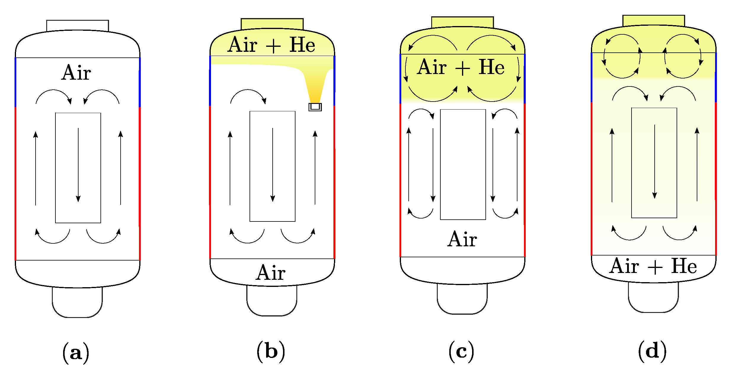
M denotes the total mass of the fluid domain. Due to the thermal boundary conditions, natural convection develops within the cavity and the helium stratification is eroded. This mixing process continues until a homogeneous mixture finally forms. The achievement of this state can be quantified by the mixture uniformity σ X , which is the volume-weighted standard deviation of the mole fraction X from the homogeneous equilibrium state mole fraction X ¯ over the whole fluid domain. The initial mixture uniformity σ X 0 is the highest occurring standard deviation during the mixing process. When varying the initial mole fraction difference Δ X , the initial mixture uniformity σ X 0 changes. Therefore, for normalization, the initial mixture uniformity σ X 0 / r e f of the reference case, which corresponds to the initial conditions of a stratification with constant mole fraction, is used. Following the definition of Danckwerts [34], this gives the expression for the segregation intensity, described by the Equation (12):
I = σ X 2 σ X 0 / r e f 2 = 1 V V X X ¯ 2 d V 1 V V X 0 / r e f X ¯ 2 d V
From the segregation intensity I, the definition of the mixing intensity M = 1 I [35] can also be derived for the interpretation of the results. In the reference case, I = 1 describes a completely inhomogeneous mixture and I = 0 characterizes a completely homogeneous mixture and vice versa for the mixing intensity M . Since the initial state changes, when the mole fraction difference Δ X is varied, the initial segregation intensity I is also different and the mixture transients are consistently captured with all occuring changes. Finally, a criterion for the mixing time can be derived from I. A completely homogeneous mixture is characterized by I = 0 , and therefore by definition of an upper bound I ϵ I = 10 3 , which I has to fall below, the achievement of this state can be quantified. When considering mass transfer processes, the Fourier number F o = D r e f t / H 2 enables a dimensionless description of time, where D r e f = D 0 is the diffusion coefficient of the reference case. Hence, the time, when the homogeneous state is reached, can be described by F o ϵ = D r e f t ϵ / H 2 . The time-dependent quantities described above are combined to the result variables vector R , where the bold notation indicates a vector or matrix.
R = N u l e f t N u r i g h t N u b o t t o m N u t o p E k I
Together with F o ϵ , additional scalar quantities that describe the mixing process were derived. For this purpose, the integral mean value R ˜ of the described quantities R (Equation (13)) is formed over the respective mixing time in Equation (14).
R ˜ = 1 F o ϵ 0 F o ϵ R F o d F o
Next to the actual integral mean value over the mixing process, this also provides a measure of the shape of the mixing transient because transients, which can be mapped on each other by linear stretching or compression of the time coordinate, have an identical integral mean value. Therefore, occurring deviations also indicate a change in the shape of the mixing transient. Because different transients can have the same integral mean value R ˜ , the mean absolute deviation R ^ from the reference case over the reference mixing time F o ϵ / r e f was therefore defined in Equation (15).
R ^ = 1 F o ϵ / r e f 0 F o ϵ / r e f R F o R r e f F o d F o
All differences in the mixing transient are captured over the mixing time of the reference case and provide a good measure for the variability. At the same time, it can be determined how big the difference between the adiabatic configuration and a configuration with temperature specification is. Finally, all variables under investigation are summarized in a matrix in Equation (16).
R ̲ = R ˜ F o ϵ R ^ 0 = N u ˜ l e f t N u ˜ r i g h t N u ˜ b o t t o m N u ˜ t o p E ˜ k I ˜ F o ϵ N u ^ l e f t N u ^ r i g h t N u ^ b o t t o m N u ^ t o p E ^ k I ^ 0
The results for the reference case are different for LES and URANS. The reference values R ̲ r e f / L E S are applied to the LES results and the reference values R ̲ r e f / U R A N S are applied to the URANS results. As listed in Equation (17), the mean integral values of the reference case R ˜ r e f are applied for the normalization of the later results, since the mean absolute deviation R ^ r e f from the reference case itself is zero.
R ̲ r e f = R ˜ r e f F o ϵ r e f R ˜ r e f 0

3.3. Sensitivity Analysis

For the investigation of uncertainties, identification of the most influential parameters is of great importance, since uncertainties occurring in these parameters mainly dominate the uncertainty in the results. Variance-based methods also enable quantification of the proportion of the result uncertainty caused by individual parameters. Therefore, uncertainty analysis is closely related to sensitivity analysis. For assessment of the sensitivities, the Morris method is applied [36]. q denotes the parameter vector with the elements q i . The defined parameter space of the computational model is explored by r-trajectories, for which the initial points are gained by random sampling, and then one parameter after the other is changed step by step. The respective trajectory is described by the index j. Then, for each trajectory, the elementary effects d q i are calculated, which represent the gradient when varying the ith parameter using the forward difference. From this, the mean and modified mean of the elementary effects μ q i and μ q i * as well as the standard deviation of the elementary effects σ q i are determined. The modified mean indicates the overall effect and the standard deviation indicates nonlinear or interaction effects between the input parameters. For evaluation of the sensitivity, both parameters are important because a low value of μ q i * combined with a considerable value of σ q i means that there is a great impact in certain regions of the parameter space and that the corresponding parameter should be taken into account for the subsequent analysis. The expressions for the calculation [36] are
d q i ( j ) = R ̲ q ( j ) + Δ Θ · e q i R ̲ q ( j ) Δ , μ q i = 1 r j = 1 r d q i j , Δ = p 2 p 1 , σ q i = 1 r 1 j = 1 r d q i j μ q i 2 , μ q i * = 1 r j = 1 r d q i j ,
where e q i is the ith unit vector and the parameter step is Δ Θ = Δ Θ = p 2 ( p 1 ) Θ with the input space uniformly partitioned into the even number of levels p. Θ denotes the parameter interval width vector and Δ describes the scalar parameter step. Global sensitivity analysis requires a large number of trajectories r per parameter. However, a large number of parameters in the mixing process are involved, which might be subject to uncertainties. Therefore, the total number of parameters was divided into three parameter vectors to maintain clarity for the further steps, such that the vector of input parameters is given by q = q I q II q III with:
q I = ϑ χ ϕ , q I I = ξ θ , q I I I = T 0 c p / A i r μ A i r P r A i r c p / H e μ H e P r H e S c t P r t .
First, the most important parameters are extracted by preselection with a one-at-a-time (OAT) approach. Starting from an initial point q o a t 0 in parameter space, the parameters were changed along each orthogonal dimension with two trajectories r = 2 , respectively. The initial point was defined as follows:
q I 0 = 1.0 0.0 0.1 , q I I 0 = 1.0 0.2 , q I I I 0 = T 0 0 c p / A i r 0 μ A i r 0 P r A i r 0 c p / H e 0 μ H e 0 P r H e 0 S c t 0 P r t 0 .
q I I I 0 takes the initial values from Section 2.2 and according to Table A1. The most influential parameters were determined by assuming an identical parameter interval, which has the width of 20 percent with respect to the corresponding nominal value in each parameter. The associated values for Θ and Δ result according to Table 1. Through this definition, the parameters are varied symmetrically around the defined initial point with the assumed standard deviation σ Q in the parameters according to Section 3.4. The standard deviation is representative for the total dispersion around the mean, and in this way, an estimation for the mean impact of single parameters is achieved.
From the results, the modified mean μ q i * can be obtained. The standard deviation σ q i was not taken into account here, as the number of trajectories is small. Here, the main criterion for the evaluation of the sensitivity was the mixing time measured by the dimensionless Fourier number F o ϵ = D r e f t ϵ / H 2 . It can be seen in Figure 8 that the material values such as the heat capacity c p / A i r and c p / H e , the dynamic viscosities μ A i r and μ H e , as well as P r H e have no great influence on the mixing time for R a = 2 × 10 9 . Additionally, the model coefficients of the gradient flux approach S c t and P r t do not show major impacts on the mixing time. On the other hand, P r A i r causes a medium impact, since the main proportion of the mixture is air. However, it is assumed that there is a small uncertainty in the prediction of material values. The thermal boundary conditions via ϑ , ϕ , and θ show great influence on the mixing time, as the mixing process is primarily based on buoyancy effects. The diffusion coefficient via ξ also leads to a large deviation. The change in the helium stratification through χ also causes relevant differences in the mixing time.
On the basis of these findings, the five most important parameters were selected. These are investigated next by Global Sensitivity Analysis (GSA) using the Morris method according to Equation (18). Consequently, the parameter vector, which contains the prioritized parameters, gives the following expression:
q m o r r i s = q I q I I = ϑ χ ϕ ξ θ
The input space is uniformly partitioned into four levels p = 4 . For the parameter intervals in Table 2 scaled to [ 0 , 1 ] , this results in the scalar parameter step Δ = 2 / 3 . A random initial point q m o r r i s 0 is chosen from the set { 0 , 1 / ( p 1 ) , 2 / ( p 1 ) , , 1 } for each parameter. Starting from this point, the parameters are changed in an arbitrary order. The assessment of the sensitivity was conducted by r = 15 trajectories. In Table 2, the intervals under investigation are listed. The parameter intervals were defined according to the probability density functions according to Equation (31) in Section 3.4. With μ Q and σ Q denoting the expectation and standard deviation of the random input variables Q , the interval was defined by [ μ Q 2 σ Q , μ Q + 2 σ Q ] as it contains the majority of all possible parameter values. The aim of this study was to capture local interaction effects and possible nonlinearities using a reasonable number of trajectories. With a constant number of levels p, a wide interval width would lead to larger parameter steps, which cause less accurate prediction of local effects. For this reason, the parameter intervals were chosen in this way.
All previously described result variables according to Section 3.2 are examined. The integral mean Nusselt number N u ˜ 
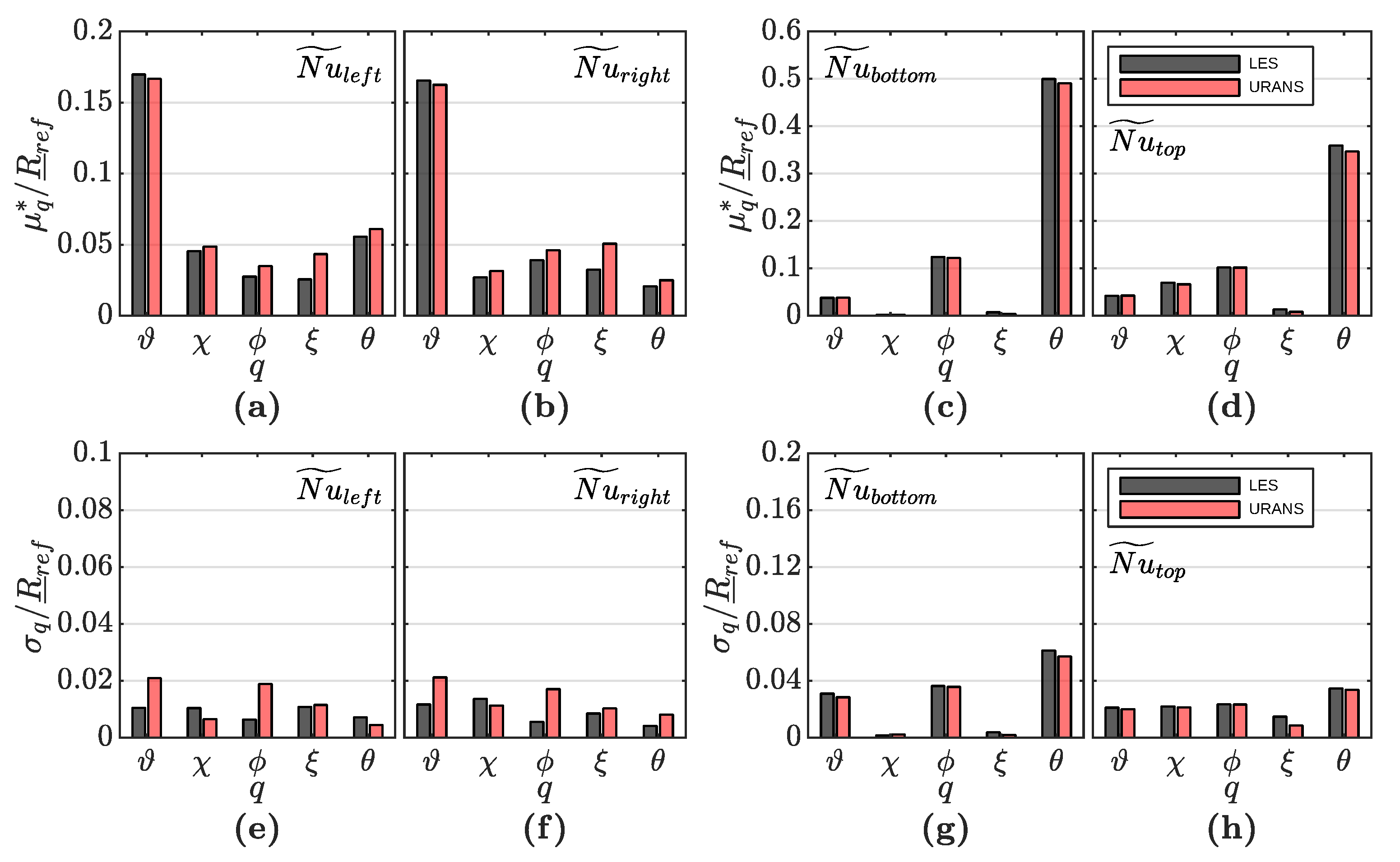
measures the convective heat transfer between the fluid and the enclosing walls during the mixing process, which significantly influences the mixing process. Heat is supplied on the left wall and dissipated on the right wall. Cold gas coming from the right wall is heated by the lower wall and hot gas coming from the left wall is cooled by the upper wall. N u ˜ l e f t and N u ˜ r i g h t , which are shown in Figure 9a,b, exhibit the biggest change through the temperature specification of the associated walls via ϑ because this simultaneously causes a change in the wall adjacent temperature gradient. The remaining parameters show medium impact, which is comparable for these parameters, when the values of the respective opposite walls are considered averaged with each other. LES and URANS show almost linear behavior regarding the integral mean Nusselt number in Equation (14), as can be seen in Figure 9e,f. Both approaches show good agreement. Additionally, for N u ˜ b o t t o m and N u ˜ t o p , which are shown in Figure 9c,d, the corresponding temperature specification via θ causes the greatest influence. The influence of χ is greater at the top wall than at the bottom wall because the helium is initially placed at the top and thus causes an influence during the mixing process. ξ leads to the smallest impact for this case. In comparison to the left and right walls, σ q i has larger values for the bottom and top walls. There is good correspondence between LES and URANS for both μ q i * and σ q i at the bottom and top walls.
N u ^ is a quantity for measuring any occurring temporal local deviation in the convective heat transfer from the reference case and thus provides information about the influence of the parameters over the whole mixing transient. The results depicted in Figure 10 show a similar trend to that for N u ˜ . Therefore, the conclusions from N u ˜ can be transferred to the results for N u ^ . An important difference exists for the measure σ q i , which captures nonlinear effects. The target function R ^ according to Equation (15) evaluates the enclosed area between the mixing transients. Hence, nonlinear effects arise in the case of a strongly nonlinear profile of the transient if it is shifted through a shorter mixing time. In addition, longer mixing transients are cut off when the mixing time of the reference case is reached, which also results in nonlinearities. This fact explains the higher values in σ q i . This approach was chosen because the fixed integration interval enables consistent normalization. An integration interval with the mixing time of the respective case would cause identical nonlinear effects with no consistent normalization opportunity. Defining a long integration interval that contains all mixing times has the disadvantage that steady-state values are taken into account, which are irrelevant for the mixing process and therefore falsify the results. The evaluation according to Equation (15) has minor drawbacks and therefore offers a good basis for the evaluation.
The thermal boundary conditions via ϑ , θ , and ϕ have great impact on the integral mean global kinetic energy during the mixing process E k ˜ , as can be seen in Figure 11a. The remaining parameters show minor impact. E k ˜ also behaves almost linearly when the parameters are changed, as can be seen in Figure 11c. In contrast to E ˜ k , the other parameters also show noticeable influence for the deviation in kinetic energy from the reference case E k ^ , shown in Figure 11b. This is due to the fact that, although the integral mean kinetic energy E k ˜ remains the same by changing these parameters, the mixing time changes relative to the reference case and this leads to the measured deviation. σ q i in Figure 11d correlates to μ q i * , since the target function itself is nonlinear, and consequently, larger change yields greater associated nonlinearity.
The duration of the entire mixing process is measured by the mixing Fourier number F o ϵ . As can be seen in Figure 12a, the associated modified mean μ q i * is greatest for ϑ and ξ . μ q i * has a comparable order of magnitude for the other parameters, but ϕ and χ have slightly higher μ q i * than θ . In Figure 12d, the nonlinearities or interaction effects are largest for ϑ , ϕ , and ξ . When ϕ is changed, larger interaction behavior or nonlinearities occur with URANS compared to LES, as can be seen from σ q i . In summary, LES and URANS show comparable sensitivity with regard to the mixing time.
The change in shape or rather the integral mean segregation intensity I ˜ according to μ q i * in Figure 12b is largely determined by χ because the initial distribution of the helium mole fraction varies. This is reflected in the mixing behavior and the shape of the mixing transient. The remaining parameters show medium impact, and the shape of the mixing transient is mostly retained. The conclusions from F o ϵ can largely be applied to the mean absolute deviation in the segregation intensity I ^ . ϑ and ξ have the greatest influence, as they also have the greatest influence on F o ϵ . Hence, the change in these parameters shifts the mixing transients regarding time and consequently increases I ^ . The larger values for σ q i in Figure 12f are due to the nonlinearity effects of the target function R ^ , which has already been discussed.
Since a large number of parameters enormously increases the required computing resources for the investigation of uncertainties, three of the remaining parameters will be examined further. The mixing Fourier number F o ϵ was selected as the main criterion to pick the most relevant parameters. The characteristic temperature difference via ϑ has the greatest importance for the buoyancy-driven mixing process. χ and ϕ have slightly higher impact than θ . For this reason, ϑ , χ , and ϕ were chosen for the uncertainty quantification. The diffusion coefficient via ξ has also great importance for the mass transfer. For the application to a binary mixture, however, it is assumed that the diffusion coefficient can be described sufficiently accurate by a dynamic model and is subject to minor uncertainties. Therefore, this parameter is also neglected in the following considerations.

3.4. Uncertainty Quantification

Based on the preceding sensitivity analysis in Section 3.3, the propagation of uncertainties in one initial condition, which is represented by the change in the initial mole fraction difference of the helium stratification through χ , and two thermal boundary conditions, which are represented by the change in the characteristic temperature difference through ϑ and the change in the wall tangential temperature gradient through ϕ , were investigated.
The open-source software Dakota 6.10 [37] was used as the uncertainty quantification framework. For the evaluation with LES and URANS, non-intrusive Polynomial Chaos Expansions (PCE) were applied because of the high convergence rate of the stochastic results with an increasing number of simulation runs. Therefore, very accurate results can potentially be obtained even with a small number of calculations. The random input variables Q : Ω Υ R n are functions that map events ω Ω from the sample space Ω to realizations q Υ . PCE is a spectral method in which random response functions R ̲ ω are described by suitable multidimensional orthogonal polynomials Ψ j Q as a function of the random input variables  Q . With a sequence { Q i ω } i = 1 of random variables, the infinite expansion results in expression Equations (22) and (23) [38,39]:
R ̲ ω = R ̲ Q = a 0 B 0 + i 1 = 1 a i 1 B 1 Q i 1 + i 1 i 2 i 1 a i 1 i 2 B 2 Q i 1 , Q i 2 +
R ̲ ω = j = 0 α j Ψ j Q 1 , Q 2 ,
R ̲ P ω = j = 0 P α j Ψ j Q 1 , Q 2 , , Q n = j = 0 P α j Ψ j Q
There is a one-to-one correspondence between the PCE coefficients a i 1 i 2 i n and α j and between the multidimensional orthogonal polynomials B n Q i 1 , Q i 2 , , Q i n and Ψ j Q . In Equation (22), each additional set of nested summations designates a collection of polynomials with increasing order. Term-based indexing in Equation (23) instead of order-based indexing simplifies the expression. Finally, a limited number of random variables n and order truncation leads to Equation (24) with P summation terms. According to [39], the orthogonal polynomials are generated numerically by using Gauss–Wigert [40], discretized Stieltjes [41], Chebyshev [41], or Gramm–Schmidt [42] approaches. The Gauss points and weights are computed by the Golub–Welsch [43] tridiagonal eigensolution. This allows us to define arbitrary probability density functions for the input variables and eliminates the need to induce additional nonlinearity through variable transformations. The PCE coefficients α j are estimated here by using spectral projection. The orthogonality property of the polynomials helps to extract each coefficient. The following expression [38], which contains the inner product · , · ϱ on Υ with the weight ϱ Q q , gives the coefficients by
α j = 1 γ j E R ̲ Q Ψ j Q = 1 γ j R ̲ , Ψ j ϱ = 1 γ j Υ R ̲ q Ψ j q ϱ Q q d q ,
where ϱ Q q = i = 1 n ϱ Q i q i is the joint probability density (weight) function. The inner product γ j = Ψ j , Ψ j ϱ can be computed analytically. For solving the multidimensional integral in Equation (25), the discrete projection, which is also termed pseudospectral, is applied. The multidimensional integral can be approximated by a tensor product of one-dimensional quadrature formulas. A one-dimensional quadrature operator with the level l N + , the quadrature points q l k = q l 1 , , q l K l , and a function f C α gives the following expression [38]:
U l ( 1 ) f q = k = 1 K l f q l k w l k
For the multivariate case n > 1 and a multi-index l = l 1 , , l n N + n with l = i = 1 n l i , the full tensor product quadrature formula results in Equation (27) [38].
Q l ( n ) f q = U l 1 ( 1 ) U l n ( 1 ) f q = k 1 = 1 K l 1 k n = 1 K l n f q 1 k 1 , , q n k n w l 1 k 1 w l n k n
However, for evaluation of this full tensor product, a very large number of function evaluations is required. Therefore, multi-dimensional integration by the Smolyak sparse grid method [44] according to Equation (28) is performed, which tremendously reduces the number of quadrature points while a high accuracy is preserved. The sparse grid quadrature rule is defined by the following expression [38,39]:
A m , n f q = m + 1 l m + n 1 m + n l n 1 m + n l · U l 1 ( 1 ) U l n ( 1 ) f q
The expression before the tensor product is a binomial coefficient, which is defined as follows:
n 1 m + n l = n 1 ! m + n l ! l m 1 !
The dimension independent maximum sparse grid level m controls the number of function evaluations and the associated accuracy of the PCE. The PCE is built through a linear combination of separate tensor polynomial chaos expansions for each underlying tensor quadrature grid [45]. Summation of the expansion terms is conducted with the Smolyak combinatorial coefficient in Equation (28). This improves accuracy in the coefficient estimation and preserves the consistency of the PCE [39].
In the present investigation, a sparse grid level m = 2 is considered and closed fully nested Clenshaw–Curtis points are applied for quadrature. Univariate and bivariate effects in R ̲ are modeled with orthogonal polynomials of highest-order a = 4 , resulting from the PCE construction according to [45]. Therefore, together with the GSA in Section 3.3, which shows the approximately linear or low nonlinear behavior of R ̲ , the results are assumed to be sufficiently accurate.
For the subsequent uncertainty analysis, a three-dimensional parameter space n = 3 with the parameter vector q s p a r s e g r i d s contains the prioritized parameters in the following expression:
q s p a r s e g r i d s = q I = ϑ χ ϕ
The initial and boundary conditions are often not exactly known and are therefore subject to uncertainties. Next to the initial conditions, the boundary conditions enable the unambiguous solution of a partial differential equation regarding space and time. However, in case of the Navier–Stokes equations, inherent uncertainties in the boundary conditions arise due to the interaction of turbulent fluctuations with the boundary. For this reason, a normal distribution for uncertainty in the characteristic temperature difference through ϑ was defined according to the central limit theorem, which states that many independent random effects lead to normal distribution. The uncertainty of the wall tangential temperature gradient through ϕ was defined to follow a log-normal distribution, which also in the course of the central limit theorem represents the distribution that results from the product of many positive independent random variables. The temperature gradient represents the temperature profile at the boundary that is established by the counterflow heat exchanger in the application case and since the supplied heat from the heat exchanger is always positive, the assumption of a log-normal distribution was made. In addition, the injection process creates large uncertainties in the actual build-up of helium stratification due to the turbulent flow of the gas stream through the injection nozzle. Hence, for the initial condition through χ , a half normal distribution was also assumed because, if the stratification is stable, the density decreases in the vertical direction. The random variables for the realizations ϑ , χ , and ϕ are Γ , Λ , and Φ . The random vector of parameters is Q = ( Γ , Λ , Φ ) . The standard deviation of Γ and Φ was assumed to be σ Q = 0.1 . For Λ , the standard deviation is defined with σ Q = 0.2 since a large uncertainty in the structure of the stratification is assumed. N μ , σ 2 and LN μ , σ 2 denotes a normal distribution and a log-normal distribution with expectation μ and variance σ 2 . TN μ , σ 2 , a , b denotes a truncated normal distribution with a and b as the lower and upper bounds. The corresponding probability density functions f Q q of the uncertain input parameters are then as follows:
Γ N 1 , 0 . 1 2 Λ TN 0 , 0 . 2 2 , 0 , 1 Φ LN 0.1 , 0 . 1 2
After the propagation of these uncertainties, the probability density functions (PDF) f R ̲ R ̲ , the expansion mean μ R ̲ = E R ̲ , and the standard deviation σ R ̲ = var R ̲ for LES and URANS were determined. In Appendix B, the first-, second- and total-order Sobol indices are listed in Table A3, Table A4 and Table A5 respectively. Thus, the uncertainties in the responses can be apportioned to the uncertainties in the input parameters. f R ̲ R ̲ was determined by sampling on the PCE approximation considering the input probability density functions f Q q . The mean μ R ̲ , standard deviation σ R ̲ , and Sobol indices were computed analytically from the PCE coefficients α j .
When comparing the mean values and the standard deviations in Table 3, it is noticeable that the results for μ R ̲ and σ R ̲ largely coincide for LES and URANS. With · and · denoting the mean and absolute value, respectively, the difference can be quantified in summary by the mean relative deviation of URANS from LES regarding the statistical moments in Table 3 with μ R ̲ U R A N S μ R ̲ L E S / μ R ̲ L E S and σ R ̲ U R A N S σ R ̲ L E S / σ R ̲ L E S , which are 0.055 and 0.092 respectively. From this, good agreement of both approaches becomes visible. However, when considering the probability density functions, correspondence and deviations between LES and URANS become clear in more detail. A part of the interpretation of the results is based on the fact that, if the first-order Sobol index S q i is large with respect to an input variable and the response function additionally shows linear behavior regarding this parameter, then the result variable approximately shows a similar distribution type I Q , as defined for the input variable. Considering the affine model for the approximation of a single response (Equation (32)), for which the variance is predominantly determined by one input variable, the shape of the probability density function after propagation remains approximately the same whereas the expectation and variance change. From this, conclusions can be made and the plausibility of the results can be checked.
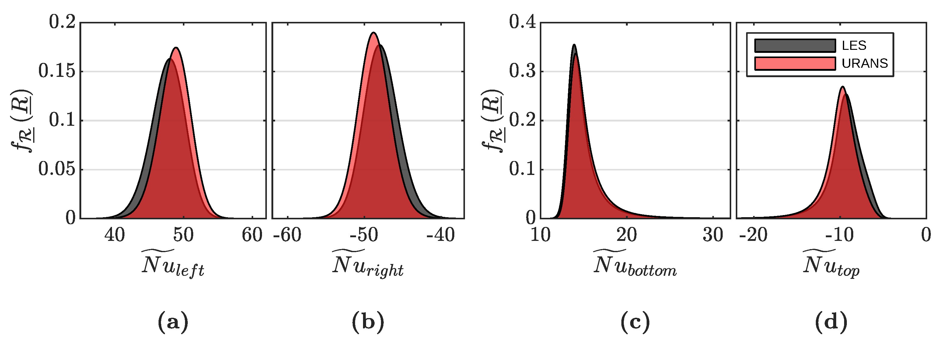
R ̲ A Q + B I Q A μ Q + B , A 2 σ Q 2
Starting with N u ˜ l e f t and N u ˜ r i g h t in Figure 13a,b, it is noticeable that the shape of the PDF is similar to a normal distribution. This is the case because the variance is predominantly caused by the temperature specification at the left and right walls via ϑ , as can be seen from the first-order Sobol indices S q i in Table A3, and shows a nearly linear behavior that becomes visible due to the low interaction behavior through the second-order Sobol indices S q i q j in Table A4 and a low σ q i in Figure 9e,f. The distribution for N u ˜ b o t t o m tends towards a log-normal distribution. As can be seen in Table A3, the variance is predominantly determined by the wall-tangential temperature gradient via ϕ , which was specified with a log-normal distribution. For this reason, a similar distribution for the result originates. For N u ˜ t o p , the effects of χ also become visible. Increasing χ enlarges the amount of helium at the top wall. Due to the lower density of helium, this attenuates the erosion at the top wall. This results in a lower convective heat transfer in this region. This creates the superimposed distribution based on the effects of ϕ and χ , shown in Figure 13d. When comparing LES and URANS, the probability density distributions in Figure 13 and the statistical moments in Table 3 are in very good agreement. If taking LES as a reliable reference, the absolute value of the Nusselt number for URANS is slightly overestimated on the left, right, and top walls.
The distributions for N u ^ l e f t and N u ^ r i g h t in Figure 14a,b, approximately resemble the shape of a chi-distribution because the response function evaluates the absolute difference between the mixing transients. Analogous to N u ˜ , the variance primarily arises through the variance in the temperature at the left and right walls, which is normally distributed and dominates the distribution of the response. This can be seen in Table A3 by means of the first-order Sobol indices S q i . The distributions of URANS and LES are in good agreement. The distributions for the top and bottom walls in Figure 13c,d and Figure 14c,d are nearly the same as that for N u ˜ because the top and bottom walls are adiabatic for the reference case, and this results in the integral deviation from the abscissa.
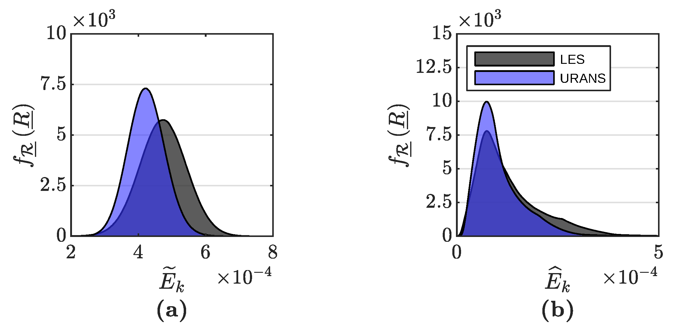
In Figure 15a, a normal distribution also arises for the PDF of E k ˜ , as again the temperature on the left and right walls via ϑ causes the major variance, as can be seen with S q i in Table A3. The global kinetic energy E ˜ k is underestimated with URANS and leads to longer mixing times F o ϵ in Figure 16a since the mixing process is dominated by the arising natural convection. The distribution for LES is wider than for URANS because LES captures most of the turbulent structures. The larger amount of the standard deviation also explains the larger deviation from the reference case E ^ k for LES in Figure 15b. By taking the LES as reference, the results for E ^ k indicate that URANS is able to predict the variability of E k at R a = 2 × 10 9 due to the parameter uncertainties.
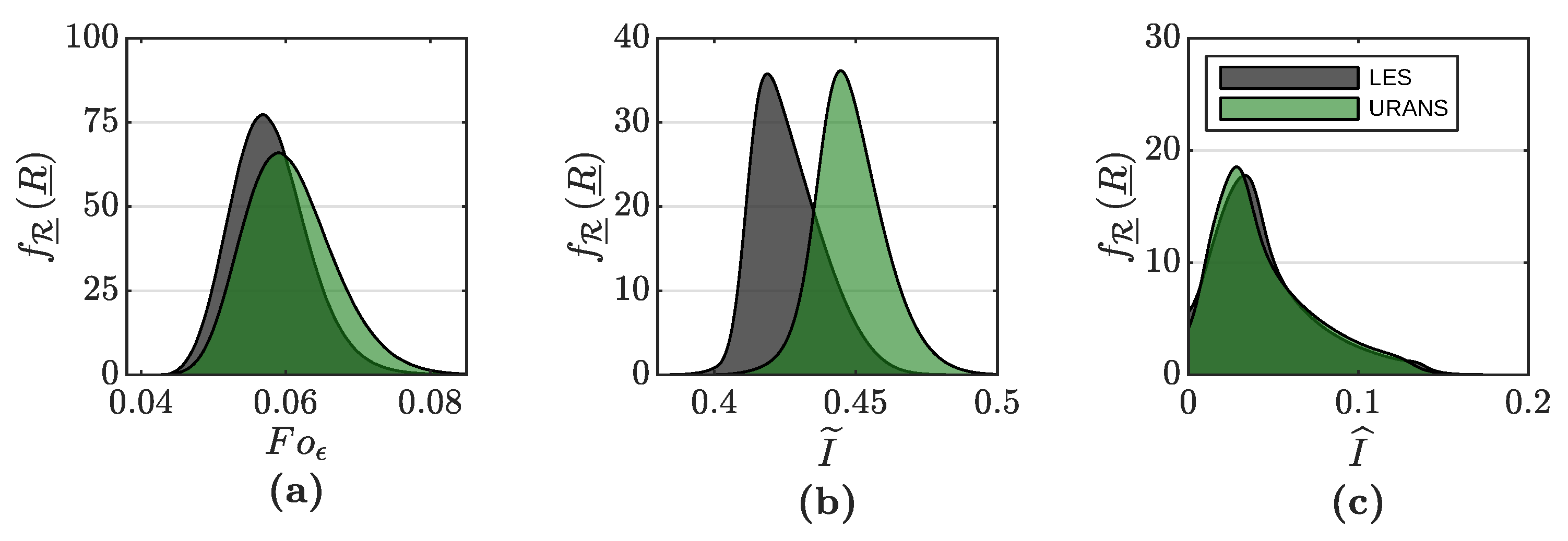
In Figure 16a, the shape of the PDF for F o ϵ resembles a normal distribution due to the large influence of ϑ for both LES and URANS, as can be seen with S q i in Table A3. Low values for σ q i in Figure 12d and S q i q j in Table A4 indicate the approximately linear behavior of F o ϵ . In comparison to URANS, LES predicts shorter mixing times and causes a smaller width of the distribution, which also can be measured by the smaller mean value μ R ̲ and standard deviation σ R ̲ in Table 3. The distributions for I ˜ in Figure 16b tend towards larger values, as can be seen especially for the LES results. This tendency arises from the truncated normal distribution for the linear stratification parameter χ , which increases the segregation intensity and causes the largest proportion of variance, as indicated by S q i in Table A3. The variance component including the smaller values mainly arises from the remaining parameters ϑ and ϕ . In contrast to the larger integral mean μ R ̲ of the segregation intensity I ˜ in URANS, the results indicate that LES has a higher mixing intensity M ˜ whereas the width of the distributions is almost identical. The shorter mixing time measured by F o ϵ for LES and the clear difference in I ˜ between LES and URANS arises since the more resolved convection in LES, which might not be represented sufficiently accurate by the turbulence model in URANS, results in a more accurate prediction of mass transfer, since anisotropic large-scale eddies have a large influence on the mixing process. The deviation from the reference case I ^ , which provides a good measure for the variability of the results when the parameters change, shows very good agreement between LES and URANS.

4. Conclusions

In this paper, a methodology for the assessment of uncertainties of Large Eddy Simulation (LES) and Unsteady Reynolds-Averaged Navier–Stokes (URANS) for the buoyancy-driven mixing process between two miscible fluids at R a = 2 × 10 9 was presented, starting from the preceding mesh convergence study and sensitivity analysis to the actual uncertainty quantification. For this purpose, an initial stratification with 40 vol % helium was defined in the upper third of the Differentially Heated Cavity (DHC) in addition to air. From the investigation, the parameters that have significant influence on the mixing process were identified and it was found that there is good agreement between LES and URANS for R a = 2 × 10 9 regarding the final stochastic results.
The mesh convergence study provides an approach for meshing the fluid domain by means of linear expansion factors, which allows for systematic determination of the required wall normal resolution with the number of cells in the boundary layer n ¯ δ u / i p and n ¯ δ T / g r a d and the required wall tangential resolution with the dimensionless cell widths Δ x + and Δ y + , which can be transferred to other engineering applications underlying similar physics. The applied convergence criteria MAE LES , DNS avg N u / avg N u D N S y ϵ M A E 10 2 containing the relative mean average error (MAE) between the results for the local Nusselt number received from LES and DNS ensures sufficiently accurate reflection of the global characteristics. This condition is fulfilled from a wall tangential resolution of Δ x + , Δ y + = 30 and boundary layer resolution of n ¯ δ u / i p = 7.87 and n ¯ δ T / g r a d = 10.10 .
As a prelimary step for the uncertainty analysis, the number of relevant parameters was reduced by using a one-at-a-time (OAT-) method, in which all parameters were varied step by step starting from an initial point. It was found that the thermal boundary conditions, such as the temperature of the enclosing walls and the wall tangential temperature gradient at the vertical walls, are of essential importance, as the mixing process is primarily driven by buoyancy effects. In addition, the initial build-up of the helium stratification shows significant influence on the mixing process. Additionally, the diffusion coefficient for mass transfer causes large changes. Therefore, these parameters were examined in more detail by global sensitivity analysis using the Morris method to show more precise statements about the sensitivity of the response function to the different parameters and possible nonlinear effects or interaction behavior. In summary, it can be seen that the sensitivity behavior of LES and URANS is qualitatively comparable with moderate quantitative deviations at R a = 2 × 10 9 .
The propagtion of the uncertainty in selected parameters was eventually investigated with Polynomial Chaos Expansions (PCE). For the determination of the expansion-coefficients, the spectral projection approach was applied. The multi-dimensional integration was conducted by the Smolyak sparse grid method. The probability density functions (PDF) and Sobol indices elucidate slight differences between LES and URANS. The heat transfer, which is measured by the Nusselt number, is well predicted with URANS in comparison to LES. However, the global kinetic energy and associated convective mass transport shows differences between LES and URANS. This results in different mixing times and mixing intensity. If LES can be regarded as a suitable reference, URANS with the currently used turbulence model predicts a slightly incorrect mixing behavior and small deviations in the LES for the variability of the result variables exist. The deviations are probably caused by the greater limitation of degrees of freedom of the URANS equations, which complicates the accurate prediction of internal buoyancy-driven mixing processes. Turbulence has a decisive influence on the mass transport and deviations directly imply effects on the natural convection flow. According to Section 3.4, the mean relative deviation between LES and URANS for the statistical moments is small. While the PDFs indicate that discernable differences arise between the uncertainty analysis based on URANS and LES, there is still reasonable agreement in most of the statistical moments. In summary, the resource-efficient URANS is suitable as a lower-fidelity model for the prediction of the input uncertainties propagation at R a = 2 × 10 9 for the investigated mixing process based on the reference analysis conducted with LES. Future work will extend the investigations to higher Rayleigh numbers comparable to the THAI application as well as the THAI large-scale facility itself.

Author Contributions

Conceptualization, M.K. and S.K.; formal analysis, P.J.W.; investigation, P.J.W.; methodology, P.J.W. and M.K.; software, P.J.W. and S.K.; supervision, M.K. and S.K.; visualization, P.J.W.; writing—original draft preparation, P.J.W.; writing—review and editing, M.K., S.K. and R.J. All authors have read and agreed to the published version of the manuscript.

Funding

This research was funded by the German Ministry of Economics and Technology (BMWi) project number 1501595 on the decision of the German Bundestag. The computational resources for this project have been provided by the Gauss Centre for Supercomputing/Leibniz Supercomputing Centre under the project name pn29ce.

Conflicts of Interest

The authors declare no conflict of interest.

Appendix A. Parameters for Case Definition

Additional parameters regarding the thermophysical properties of the fluids under consideration as well as the physical and numerical discretization parameters are listed in Table A1 and Table A2, respectively.
Table A1. Applied material properties of air and helium.
GasMole Weight MIsobaric Heat Capacity C p Dynamic Viscosity μ Prandtl Number Pr
air [28] 28.96   g mol 1 1006.5   J   K 1 1.845 × 10 5 Pa s 0.707
helium [46] 4.0   g mol 1 5193   J   K 1 1.985 × 10 5 Pa s 0.664
Table A2. Physical and spatial discretization parameters.
Ra N x N y N z Δ x c Δ x + Δ y c Δ y + φ WD
2 e 9 4422034 24.439 9.209 1.0

Appendix B. Results for the Variance-Based Decomposition

Complementing the results presented in Section 3.4 for the uncertainty quantification, the corresponding first-, second-, and total-oder Sobol indices are listed in Table A3, Table A4 and Table A5, respectively. This gives insight into how uncertainties in the responses are apportioned to the uncertainties in the input parameters. The Sobol indices [38] are defined as
S q i = D i D = var E R ̲ | q i var R ̲ , S q i q j = D i j D = var E R ̲ | q i , q j var E R ̲ | q i var E R ̲ | q j var R ̲ , S T q i = 1 var E R ̲ | q i var R ̲ = E var R ̲ | q i var R ̲ ,
where D, D i , and D i j are the total and partial variances in the response R ̲ . The notation q i = q 1 , , q i 1 , q i + 1 , , q n denotes the parameter vector having all components of q except those in the set i.
Table A3. First-order Sobol indices S q i for the random response R ̲ .
LESURANS
R ̲ S ϑ S χ S ϕ S ϑ S χ S ϕ
N u ˜ l e f t 0.85500.10830.03590.83920.11610.0441
N u ˜ r i g h t 0.87860.04730.07340.84710.05430.0978
N u ˜ b o t t o m 0.0310 7.4810 × 10 4 0.96760.0319 1.8460 × 10 4 0.9673
N u ˜ t o p 0.06490.23820.69480.05580.22540.7175
N u ^ l e f t 0.77410.16190.00480.73010.20860.0032
N u ^ r i g h t 0.79790.11060.00490.71790.16570.0050
N u ^ b o t t o m 0.02130.00120.97680.0308 2.4910 × 10 4 0.9684
N u ^ t o p 0.18960.22950.57230.19620.22420.5736
E ˜ k 0.94540.00230.04930.9788 3.3030 × 10 4 0.0201
E ^ k 0.86120.01470.01150.85080.02580.0067
F o ϵ 0.89400.03430.07020.90270.03480.0624
I ˜ 0.00610.90940.07710.12700.70630.1624
I ^ 0.64290.21370.02380.62750.24200.0190
Table A4. Second-order Sobol indices S q i q j for the random response R ̲ .
LESURANS
R ̲ S ϑ χ S ϑ ϕ S χ ϕ S ϑ χ S ϑ ϕ S χ ϕ
N u ˜ l e f t 5.3040 × 10 4 2.5950 × 10 4 4.6230 × 10 5 0.0252 4.4470 × 10 4 9.5290 × 10 4
N u ˜ r i g h t 4.2520 × 10 4 6.0350 × 10 4 8.2280 × 10 5 0.0275 4.9870 × 10 4 0.0010
N u ˜ b o t t o m 4.2090 × 10 5 0.0011 8.2600 × 10 5 4.1120 × 10 5 0.0010 6.7580 × 10 6
N u ˜ t o p 0.0010 2.6460 × 10 4 2.8610 × 10 4 0.0168 4.9460 × 10 4 9.8280 × 10 4
N u ^ l e f t 0.05810.00160.00130.08610.00130.0025
N u ^ r i g h t 0.10280.00440.00460.13450.00430.0112
N u ^ b o t t o m 3.4510 × 10 5 0.0014 6.8360 × 10 5 2.3570 × 10 4 9.5770 × 10 4 3.6120 × 10 5
N u ^ t o p 0.00110.00170.00520.02880.00520.0086
E ˜ k 1.6030 × 10 4 0.0023 3.8430 × 10 5 0.06040.01530.0036
E ^ k 0.06350.0663 4.6140 × 10 4 0.07960.02070.0258
F o ϵ 3.3040 × 10 4 5.0210 × 10 4 1.0890 × 10 4 0.17690.00530.0101
I ˜ 0.00280.00420.00170.09120.00700.0052
I ^ 0.09910.0233 8.1460 × 10 4 0.17430.00520.0193
Table A5. Total-order Sobol indices S T q i for the random response R ̲ .
LESURANS
R ̲ S T ϑ S T χ S T ϕ S T ϑ S T χ S T ϕ
N u ˜ l e f t 0.85570.10880.03620.83980.11640.0445
N u ˜ r i g h t 0.87920.04760.07380.84790.05450.0984
N u ˜ b o t t o m 0.0316 8.0080 × 10 4 0.96820.0326 1.9480 × 10 4 0.9679
N u ˜ t o p 0.06640.23990.69580.05690.22630.7182
N u ^ l e f t 0.83260.22010.00670.78640.26570.0060
N u ^ r i g h t 0.87910.19350.01400.81590.27250.0231
N u ^ b o t t o m 0.02200.00130.97750.0313 2.6020 × 10 4 0.9689
N u ^ t o p 0.19460.23650.57760.19990.22930.5768
E ˜ k 0.94810.00280.05200.9795 4.0750 × 10 4 0.0209
E ^ k 0.97300.07370.06590.96640.08190.0684
F o ϵ 0.89530.03530.07080.90280.03490.0624
I ˜ 0.01130.91560.08040.13120.70950.1637
I ^ 0.76220.31710.04030.73890.33370.0388

References

  1. Smith, B.L.; Andreani, M.; Bieder, U.; Ducros, F.; Graffard, E.; Heitsch, M.; Henriksson, M.; Höhne, T.; Houkema, M.; Komen, E.; et al. Assessment of CFD Codes for Nuclear Reactor Safety Problems; OECD/NEA/CSNI: Paris, France, 2014. [Google Scholar]
  2. Liang, Z.; Chan, C.K.; Sonnenkalb, M.; Bentaib, A.; Malet, J.; Sangiorgi, M.; Gryffroy, D.; Gyepi-Garbrah, S.; Duspiva, J.; Sevon, T.; et al. Status Report on Hydrogen Management and Related Computer Codes; OECD/NEA/CSNI: Paris, France, 2014. [Google Scholar]
  3. Abou-Rjeily, Y.; Cénérino, G.; Drozd, A.; Lee, S.; Misak, J.; Park, C.; Preusser, G.; Vayssier, G. Mitigation of Hydrogen Hazards in Severe Accidents in Nuclear Power Plants; Technical Report; International Atomic Energy Agency (IAEA): Vienna, Austria, 2011. [Google Scholar]
  4. Deutsche Risikostudie Kernkraftwerke-Zusammenfassung; Technical Report; Gesellschaft für Anlagen- und Reaktorsicherheit (GRS): Köln, Germany, 1989.
  5. Deutsche Risikostudie Kernkraftwerke-Phase B; Technical Report; Gesellschaft für Anlagen- und Reaktorsicherheit (GRS): Köln, Germany, 1989.
  6. Gupta, S.; Schmidt, E.; Von Laufenberg, B.; Freitag, M.; Poss, G.; Funke, F.; Weber, G. Thai test facility for experimental research on hydrogen and fission product behaviour in light water reactor containments. Nucl. Eng. Des. 2015, 294, 183–201. [Google Scholar] [CrossRef]
  7. Kelm, S.; Lehmkuhl, J.; Jahn, W.; Allelein, H.J. A comparative assessment of different experiments on buoyancy driven mixing processes by means of CFD. Ann. Nucl. Energy 2016, 93, 50–57. [Google Scholar] [CrossRef]
  8. Bestion, D.; Camy, R.; Gupta, S.; Heib, C.; Marfaing, O.; Moretti, F.; Skorek, T.; Bestion, D.; Camy, R.; Gupta, S.; et al. Requirements for cfd-grade experiments for nuclear reactor thermalhydraulics. In CFD4NRS: Computational Fluid Dynamics for Nuclear Reactor Safety; HAL: Lyon, France, 2019. [Google Scholar]
  9. Smith, B.L. The difference between traditional experiments and CFD validation benchmark experiments. Nucl. Eng. Des. 2017, 312, 42–47. [Google Scholar] [CrossRef]
  10. Bestion, D.; De Crecy, A.; Moretti, F.; Camy, R.; Barthet, A. Review of Uncertainty methods for CFD application to nuclear reactor thermalhydraulics. In NUTHOS 11: Nuclear Reactor Thermal-Hydraulics, Operation and Safety; HAL: Lyon, France, 2016. [Google Scholar]
  11. Simoneau, J.; Champigny, J.; Gelineau, O. Applications of large eddy simulations in nuclear field. Nucl. Eng. Des. 2010, 240, 429–439. [Google Scholar] [CrossRef] [Green Version]
  12. Bestion, D.; de Crécy, A.; Camy, R.; Barthet, A.; Bellet, S.; Badillo, A.; Niceno, B.; Hedberg, P.; Muñoz Cobo, J.; Moretti, F.; et al. Review of Uncertainty Methods for Computational Fluid Dynamics Application to Nuclear Reactor Thermal Hydraulics; Technical Report; OECD/NEA: Paris, France, 2016. [Google Scholar]
  13. Trias, F.X.; Soria, M.; Oliva, A.; Pérez-segarra, C.D. Direct numerical simulations of two- and three-dimensional turbulent natural convection flows in a differentially heated cavity of aspect ratio 4. J. Fluid Mech. 2007, 586, 259–293. [Google Scholar] [CrossRef]
  14. Badillo, A.; Kapulla, R. Uncertainty Quantification in CFD Simulations of Isokinetic Turbulent Mixing Layers. In Proceedings of the 15th International Topical Meeting on Nuclear Reactor Thermal-hydraulics, NURETH-15, Pisa, Italy, 12–17 May 2013. [Google Scholar]
  15. Fokken, J.; Krohn, B.; Kapulla, R.; Niceno, B.; Prasser, H.M.; Badillo, A. NEA Benchmark Exercise: Computational Fluid Dynamic Prediction and Uncertainty Quantification of a GEMIX Mixing Layer Test; OECD/NEA/CSNI: Paris, France, 2019. [Google Scholar]
  16. Cutrono Rakhimov, A.; Visser, D.C.; Komen, E.M. Uncertainty Quantification method for CFD applied to the turbulent mixing of two water layers. Nucl. Eng. Des. 2018, 333, 1–15. [Google Scholar] [CrossRef]
  17. Cutrono Rakhimov, A.; Visser, D.C.; Komen, E.M. Uncertainty Quantification method for CFD applied to the turbulent mixing of two water layers–II: Deterministic Sampling for input uncertainty. Nucl. Eng. Des. 2019, 348, 146–158. [Google Scholar] [CrossRef]
  18. Cutrono Rakhimov, A.; Visser, D.C.; Komen, E.M. Uncertainty Quantification method for CFD validated for turbulent mixing experiments from GEMIX. Nucl. Eng. Des. 2020, 358, 110444. [Google Scholar] [CrossRef]
  19. Le Maître, O.; Reagan, M.T.; Najm, H.N.; Ghanem, R.G.; Knio, O.M. A stochastic projection method for fluid flow. II. Random process. J. Comput. Phys. 2002, 181, 9–44. [Google Scholar] [CrossRef] [Green Version]
  20. Le Maître, O.; Reagan, M.T.; Debusschere, B.; Najm, H.N.; Ghanem, R.G.; Knio, O.M. Natural convection in a closed cavity under stochastic non-boussinesq conditions. SIAM J. Sci. Comput. 2005, 26, 375–394. [Google Scholar] [CrossRef]
  21. Le Maître, O.; Knio, O.M.; Najm, H.N.; Ghanem, R.G. Uncertainty propagation using Wiener-Haar expansions. J. Comput. Phys. 2004, 197, 28–57. [Google Scholar] [CrossRef]
  22. Bijl, H.; Lucor, D.; Mishra, S.; Schwab, C.; Board, E.; Barth, T.J.; Griebel, M.; Keyes, D.E.; Nieminen, R.M.; Roose, D.; et al. Uncertainty Quantification in Computational Fluid Dynamics; Springer: Cham, Switzerland, 2013. [Google Scholar]
  23. Davidson, P.A. Turbulence: An Introduction for Scientists and Engineers; Oxford University Press: Oxford, UK, 2015. [Google Scholar] [CrossRef]
  24. Kelm, S.; Kampili, M.; Liu, X.; George, A.; Schumacher, D.; Druska, C.; Struth, S.; Kuhr, A.; Ramacher, L.; Allelein, H.J.; et al. The Tailored CFD Package ’containmentFOAM’ for Analysis of Containment Atmosphere Mixing, H2/CO Mitigation and Aerosol Transport. Fluids 2021, 6, 100. [Google Scholar] [CrossRef]
  25. Nicoud, F.; Ducros, F. Subgrid-Scale Stress Modelling Based on the Square of the Velocity Gradient Tensor. Flow Turbul. Combust. 1999, 62, 183–200. [Google Scholar] [CrossRef]
  26. Menter, F.R. Two-equation eddy-viscosity turbulence models for engineering applications. AIAA J. 1994, 32, 1598–1605. [Google Scholar] [CrossRef] [Green Version]
  27. ANSYS CFX-Solver Theory Guide; ANSYS, Inc.: Canonsburg, PA, USA, 2011.
  28. Kabelac, S.; Kind, M.; Martin, H.; Mewes, D.; Schaber, K.; Stephan, P. VDI-Wärmeatlas, 11. Auflage; Springer Vieweg: Berlin/Heidelberg, Germany, 2013. [Google Scholar]
  29. Weller, H.G.; Tabor, G.; Jasak, H.; Fureby, C. A tensorial approach to computational continuum mechanics using object-oriented techniques. Comput. Phys. 1998, 12, 620. [Google Scholar] [CrossRef]
  30. OpenFOAM Documentation v1906; ESI-OpenCFD: Bracknell, UK 2019. Available online: https://www.openfoam.com/releases/openfoam-v1906 (accessed on 15 December 2020).
  31. Pope, S.B. Turbulent Flows; Cambridge University Press: Cambridge, UK, 2000. [Google Scholar]
  32. Willmott, C.J.; Ackleson, S.G.; Davis, R.E.; Feddema, J.J.; Klink, K.M.; Legates, D.R.; O’Donnell, J.; Rowe, C.M. Statistics for the evaluation and comparison of models. J. Geophys. Res. 1985, 90, 8995. [Google Scholar] [CrossRef] [Green Version]
  33. Willmott, C.J.; Matsuura, K. Advantages of the mean absolute error (MAE) over the root mean square error (RMSE) in assessing average model performance. Clim. Res. 2005, 30, 79–82. [Google Scholar] [CrossRef]
  34. Danckwerts, P.V. The definition and measurement of some characteristics of mixtures. Appl. Sci. Res. Sect. A 1952, 3, 279–296. [Google Scholar] [CrossRef]
  35. Bothe, D. Evaluating the Quality of a Mixture: Degree of Homogeneity and Scale of Segregation; Springer: Berlin/Heidelberg, Germany, 2010. [Google Scholar] [CrossRef]
  36. Morris, M.D. Factorial sampling plans for preliminary computational experiments. Technometrics 1991, 33, 161–174. [Google Scholar] [CrossRef]
  37. Adams, B.M.; Bohnhoff, W.J.; Dalbey, K.R.; Ebeida, M.S.; Eddy, J.P.; Eldred, M.S. Dakota, A Multilevel Parallel Object-Oriented Framework for Design Optimization, Parameter Estimation, Uncertainty Quantification, and Sensitivity Analysis: Version 6.10 User’s Manual; Technical Report; Sandia National Laboratories: Albuquerque, NM, USA, 2014. Available online: https://dakota.sandia.gov/content/manuals (accessed on 15 December 2020).
  38. Smith, R.C. Uncertainty Quantification: Theory, Implementation, and Applications; Society for Industrial and Applied Mathematics (SIAM): Philadelphia, PA, USA, 2013. [Google Scholar]
  39. Adams, B.M.; Bohnhoff, W.J.; Dalbey, K.R.; Ebeida, M.S.; Eddy, J.P.; Eldred, M.S. Dakota, A Multilevel Parallel Object-Oriented Framework for Design Optimization, Parameter Estimation, Uncertainty Quantification, and Sensitivity Analysis: Version 6.10 Theory Manual; Technical Report; Sandia National Laboratories: Albuquerque, NM, USA, 2014. Available online: https://dakota.sandia.gov/content/manuals (accessed on 15 December 2020).
  40. Simpson, I.C. Numerical integration over a semi-infinite interval, using the lognormal distribution. Numer. Math. 1978, 31, 71–76. [Google Scholar] [CrossRef]
  41. Gautschi, W. Orthogonal Polynomials Computation and Approximation; Oxford University Press: Oxford, UK, 2004. [Google Scholar]
  42. Witteveen, J.A.; Bijl, H. Modeling arbitrary uncertainties using gram-schmidt polynomial chaos. In Proceedings of the 44th AIAA Aerospace Sciences Meeting and Exhibit, Reno, Nevada, 9–12 January 2006; Volume 14, pp. 10695–10711. [Google Scholar] [CrossRef]
  43. Golub, G.H.; Welsch, J.H. Calculation of Gauss Quadrature Rules. Math. Comput. 1969, 23, 221. [Google Scholar] [CrossRef]
  44. Smolyak, S.A. Quadrature and interpolation formulas for tensor products of certain classes of functions. Dokl. Akad. Nauk SSSR 1963, 4, 240–243. [Google Scholar]
  45. Constantine, P.G.; Eldred, M.S.; Phipps, E.T. Sparse pseudospectral approximation method. Comput. Methods Appl. Mech. Eng. 2012, 229–232, 1–12. [Google Scholar] [CrossRef] [Green Version]
  46. Lemmon, E.; McLinden, M.; Friend, D. NIST Chemistry WebBook, NIST Standard Reference Database Number 69; National Institute of Standards and Technology (NIST): Gaithersburg, MD, USA, 2018. [CrossRef]
Figure 1. Schematic structure of the primary coolant system in a nuclear power plant and illustration of the processes after a severe nuclear reactor accident: (a) nuclear reactor with reactor facilities, (b) nuclear reactor after a severe nuclear reactor accident, (c) consecutive mechanisms occurring during a nuclear meltdown from left to right, and (d) structure of a fuel rod.
Fluids 06 00161 g001
Figure 2. Consecutive phases of the TH22-experiment: (a) initial phase, (b) injection phase, (c) start of erosion phase, and (d) final erosion phase.
Fluids 06 00161 g002
Figure 3. Sketch of the idealized configuration and THAI application case: (a) generic test case from the literature with a superimposed mixing process and (b) THAI containment with a mixing process.
Fluids 06 00161 g003
Figure 4. Investigated configurations of the Differentially Heated Cavity (DHC) with aspect ratio 4: (a) default case, (b) reference case, and (c) parameter variation case.
Fluids 06 00161 g004
Figure 5. Spatial discretization of the computational domain and mesh refinement strategy: (a) 3D mesh for Large Eddy Simulation (LES) and (b) 2D mesh for Unsteady Reynolds-Averaged Navier–Stokes (URANS). (c) Description.
Fluids 06 00161 g005
Figure 6. Mesh convergence study: (a) relative Mean Average Error (MAE) of the N u number, (b) relative MAE of the standard deviation of the N u number, (c) local N u number profile on the vertical walls, and (d) local standard deviation profile of the local N u number.
Fluids 06 00161 g006
Figure 7. Structure and spatial resolution of the boundary layer: (a) thickness of the velocity and temperature boundary layer with the indicated wall-normal mesh resolution x g r i d and (b) the number of cells in the velocity and temperature boundary layer.
Fluids 06 00161 g007
Figure 8. Normalized modified mean μ q * / R ̲ r e f for the mixing time F o ϵ for LES and URANS.
Fluids 06 00161 g008
Figure 9. Normalized modified mean μ q * / R ̲ r e f and standard deviation σ q / R ̲ r e f of the integral mean Nusselt number: (a,e) on the left wall, N u ˜ l e f t ; (b,f) on the right wall, N u ˜ r i g h t ; (c,g) on the bottom wall, N u ˜ b o t t o m ; and (d,h) on the top wall, N u ˜ t o p .
Fluids 06 00161 g009
Figure 10. Normalized modified mean μ q * / R ̲ r e f and standard deviation σ q / R ̲ r e f of the mean absolute deviation to the reference case of the Nusselt number: (a,e) on the left wall, N u ^ l e f t ; (b,f) on the right wall, N u ^ r i g h t ; (c,g) on the bottom wall, N u ^ b o t t o m ; and (d,h) on the top wall, N u ^ t o p .
Fluids 06 00161 g010
Figure 11. Normalized modified mean μ q * / R ̲ r e f and standard deviation σ q / R ̲ r e f for the responses: (a,c) for the integral mean global kinetic energy E ˜ k and (b,d) for the mean absolute deviation to the reference case of the global kinetic energy E ^ k .
Fluids 06 00161 g011
Figure 12. Normalized modified mean μ q * / R ̲ r e f and standard deviation σ q / R ̲ r e f for the responses: (a,d) for the mixing time F o ϵ , (b,e) for the integral mean segregation intensity I ˜ , and (c,f) for the mean absolute deviation to the reference case of the segregation intensity I ^ .
Fluids 06 00161 g012
Figure 13. Probability density functions for the integral mean Nusselt number: (a) on the left wall, N u ˜ l e f t ; (b) on the right wall, N u ˜ r i g h t ; (c) on the bottom wall, N u ˜ b o t t o m ; and (d) on the top wall, N u ˜ t o p .
Fluids 06 00161 g013
Figure 14. Probability density functions for the mean absolute deviation to the reference case of the Nusselt number: (a) on the left wall, N u ^ l e f t ; (b) on the right wall, N u ^ r i g h t ; (c) on the bottom wall, N u ^ b o t t o m ; and (d) on the top wall, N u ^ t o p .
Fluids 06 00161 g014
Figure 15. Probability density functions for the random responses: (a) integral mean global kinetic energy E ˜ k and (b) mean absolute deviation to the reference case of the global kinetic energy E ^ k .
Fluids 06 00161 g015
Figure 16. Probability density functions for the random responses: (a) mixing time F o ϵ , (b) integral mean segregation intensity I ˜ , and (c) mean absolute deviation to the reference case of the segregation intensity I ^ .
Fluids 06 00161 g016
Table 1. Parameter variation values for the one-at-a-time (OAT) approach.
q o a t i ϑ χ ϕ ξ
[ q o a t i a , q o a t i b ] [ 0.9 , 1.1 ] [ 0.0 , 0.2 ] [ 0.0 , 0.2 ] [ 0.9 , 1.1 ]
Θ i 0.2 0.2 0.2 0.2
Δ ± 0.5 + 0.5 / + 1.0 ± 0.5 ± 0.5
q o a t i θ T 0 c p / A i r μ A i r
[ q o a t i a , q o a t i b ] [ 0.1 , 0.3 ] T 0 0 + [ 0.1 , 0.1 ] Δ T 0 [ 0.9 , 1.1 ] c p / A i r [ 0.9 , 1.1 ] μ A i r
Θ i 0.2 0.2 Δ T 0 0.2 c p / A i r 0.2 μ A i r
Δ ± 0.5 ± 0.5 ± 0.5 ± 0.5
q o a t i P r A i r c p / H e μ H e P r H e
[ q o a t i a , q o a t i b ] [ 0.9 , 1.1 ] P r A i r [ 0.9 , 1.1 ] c p / H e [ 0.9 , 1.1 ] μ H e [ 0.9 , 1.1 ] P r H e
Θ i 0.2 P r A i r 0.2 c p / H e 0.2 μ H e 0.2 P r H e
Δ ± 0.5 ± 0.5 ± 0.5 ± 0.5
q o a t i S c t P r t
[ q o a t i a , q o a t i b ] [ 0.9 , 1.1 ] S c t [ 0.9 , 1.1 ] P r t
Θ i 0.2 S c t 0.2 P r t
Δ ± 0.5 ± 0.5
Table 2. Parameter variation values for the Morris method.
q m o r r i s i ϑ χ ϕ ξ θ
[ q m o r r i s i a , q m o r r i s i b ] [ 0.8 , 1.2 ] [ 0.0 , 0.4 ] [ 0.0 , 0.3 ] [ 0.8 , 1.2 ] [ 0.0 , 0.4 ]
Θ i 0.4 0.4 0.3 0.4 0.4
Table 3. Expansion mean μ R ̲ and standard deviation σ R ̲ for the random response R ̲ .
LESURANS
R ̲ μ R ̲ σ R ̲ μ R ̲ σ R ̲
N u ˜ l e f t 47.71002.460048.69002.3070
N u ˜ r i g h t −47.78002.2790−48.69002.1500
N u ˜ b o t t o m 14.99002.256015.24002.3140
N u ˜ t o p −9.51702.2030−9.98502.1100
N u ^ l e f t 5.21002.47904.69102.1640
N u ^ r i g h t 4.27102.20604.10001.8390
N u ^ b o t t o m 15.36002.252015.54002.3200
N u ^ t o p 9.58702.193010.04002.1270
E ˜ k 4.7310 × 10 4 6.9620 × 10 5 4.2430 × 10 4 5.4710 × 10 5
E ^ k 1.2910 × 10 4 8.2110 × 10 5 1.0430 × 10 4 5.9700 × 10 5
F o ϵ 0.05790.00540.06060.0062
I ˜ 0.42630.01180.44820.0118
I ^ 0.04440.03040.04510.0302
Publisher’s Note: MDPI stays neutral with regard to jurisdictional claims in published maps and institutional affiliations.

