
Coaxial Circular Jets—A Review


1
Faculty of Mechanical Engineering, Technion—Israel Institute of Technology, 3200003 Haifa, Israel
2
Faculty of Aerospace Engineering, Technion—Israel Institute of Technology, 3200003 Haifa, Israel
*
Author to whom correspondence should be addressed.
Fluids 2021, 6(4), 147; https://doi.org/10.3390/fluids6040147
Submission received: 11 March 2021
/
Revised: 5 April 2021
/
Accepted: 6 April 2021
/
Published: 8 April 2021
(This article belongs to the Special Issue Recent Advances in Impinging Jets)
Abstract
:This review article focuses on the near-field flow characteristics of coaxial circular jets that, despite their common usage in combustion processes, are still not well understood. In particular, changes in outer to inner jet velocity ratios, , absolute jet exit velocities and the nozzle dimensions and geometry have a profound effect on the near-field flow that is characterized by shear as well as wake instabilities. This review starts by presenting the set of equations governing the flow field and, in particular, the importance of the Reynolds stress distributions on the static pressure distribution is emphasized. Next, the literature that has led to the current stage of knowledge on coaxial jet flows is presented. Based on this literature review, several regions in the near-field (based on ) are identified in which the inner mixing layer is either governed by shear or wake instabilities. The latter become dominant when . For coaxial jets issued into a quiescent surrounding, shear instabilities of the annular (outer) jet are always present and ultimately govern the flow field in the far-field. We briefly discuss the effect of nozzle geometry by comparing the flow field in studies that used a blockage disk to those that employed thick inner nozzle lip thickness. Similarities and differences are discussed. While impinging coaxial jets have not been investigated much, we argue in this review that the rich flow dynamics in the near-field of the coaxial jet might be put to an advantage in fine-tuning coaxial jets impinging onto surfaces for specific heat and mass transfer applications. Several open questions are discussed at the end of this review.
1. Introduction
Jet flows have been widely studied in the past due to their canonical flow configuration, easy set-up and importance in many industrial applications (e.g., turbine blade and electronic equipment cooling) and natural phenomena (e.g., volcano eruptions, deep sea vents) [1]. In industrial applications, the use of impinging jet flows is especially widespread since relatively high convective heat transfer coefficients can be achieved. While impinging jets have been studied for at least the last 50 years, recently there has been much interest in manipulating the jet in order to further increase the convective heat transfer coefficients [2,3,4,5], that in non-dimensional form are characterized by the Nusselt number, Nu. However, a disadvantage of impinging jet cooling is the fast decay of local Nusselt numbers away from the stagnation point which can be alleviated by either using arrays of jets or coaxial jets that are known to result in a more uniform Nusselt number distribution [6,7].
A single, impinging circular jet issued from a nozzle has been studied extensively in the previous decades. It changes from a high speed, nearly uniform flow having thin shear layers at the nozzle’s exit to a transitional and fully developed radially expanding, turbulent wall jet after impingement. Typically, three zones can be distinguished: (i) the free jet [8], (ii) the impingement zone [9] and (iii) the radial wall jet [10]. Each of these zones is characterized by different turbulence mechanisms making it difficult to perform accurate numerical simulations [11]. Adding to the complexity of the impinging jet’s flow field is its dependence on a large number of parameters such as (i) the jet Reynolds number; (ii) the nozzle to plate distance; (iii) the jet exit velocity profile (steady or unsteady) and turbulence level [12]; (iv) the jet configuration (such as confined or not) and shape of the nozzle [13].
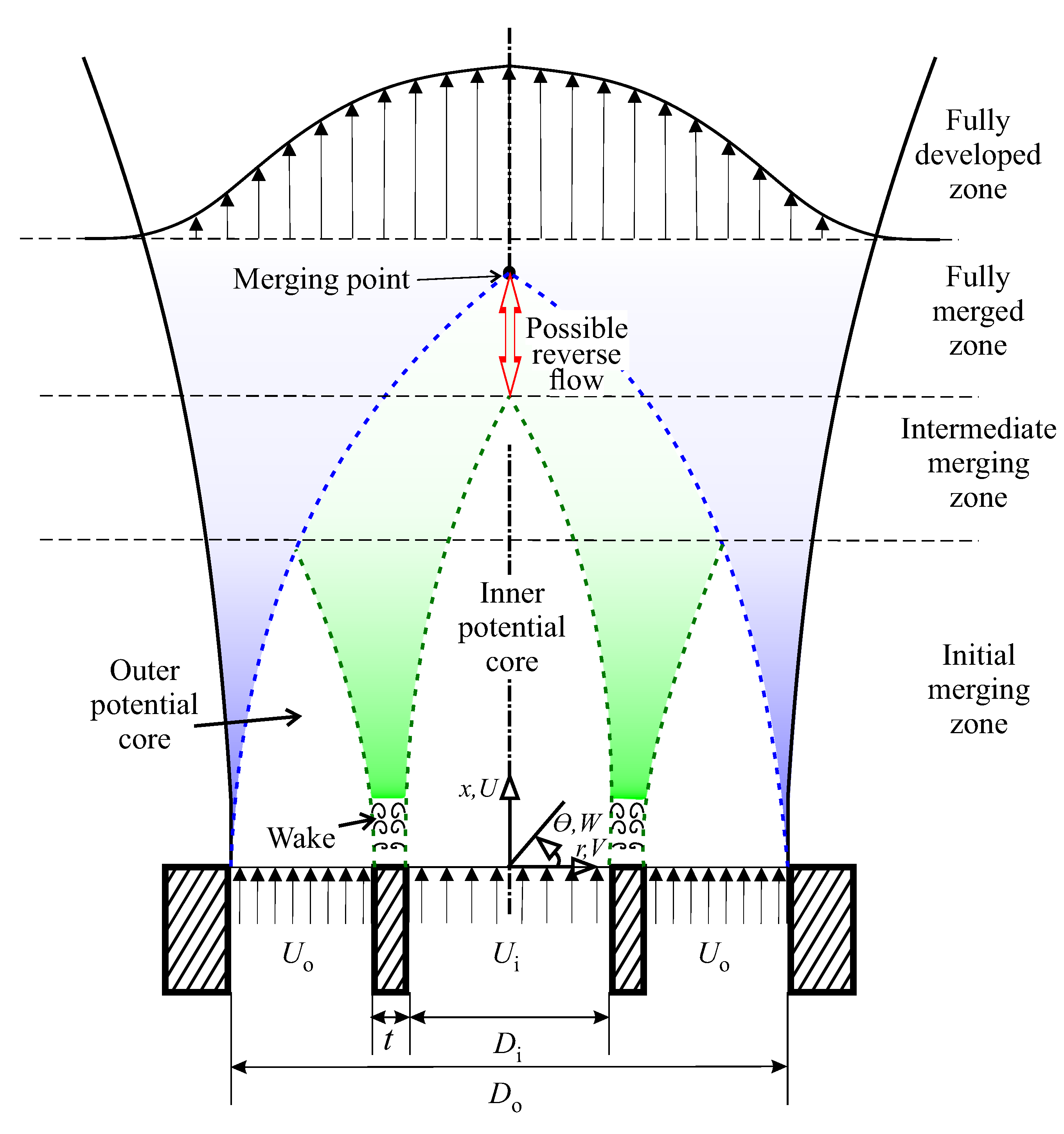
A coaxial jet is even more complex than the above described impinging circular jet, as now the circular (inner) jet interacts with an annular (outer) jet as schematically depicted in Figure 1. The inner and outer jet diameters are denoted by and , respectively; the subscripts “i” and “o” denote “inner” and “outer”, respectively. The coaxial jet is characterized by two potential core regions and the flow field exhibits both wake-like as well as shear-like instabilities [14,15]. The length of the inner potential core region depends strongly on the velocity ratio given by [16]:
where and denote the mean jet exit velocities of the outer and inner jet, respectively. This will be further discussed in Section 2.2. In contrast to the inner potential core, the length of the outer potential core only weakly depends on [16] and is essentially fixed by the diameter ratio given by:
Increasing leads to an increase in the outer potential core length and vice versa. Note that when is much lower than , the outer jet deflects towards the central axis and reverse flow may occur. As shown by Rehab et al. [16], reverse flow forms when exceeds 5 to 8 (the actual value depends on the jet exit velocity profiles). The resulting recirculation region is located between the merging point and the end of the inner potential core region (Figure 1, note that the inner potential core region is shorter than the outer one for [16]). Additional parameters pertinent to the coaxial jet are the inner and outer jet’s nozzle exit area given by:
respectively, where t is the “lip” thickness, i.e., the thickness of the inner nozzle at the exit plane (Figure 1). The area ratio is defined as:
while inner and outer jet Reynolds numbers are defined by,
respectively, where denotes the fluid kinematic viscosity.
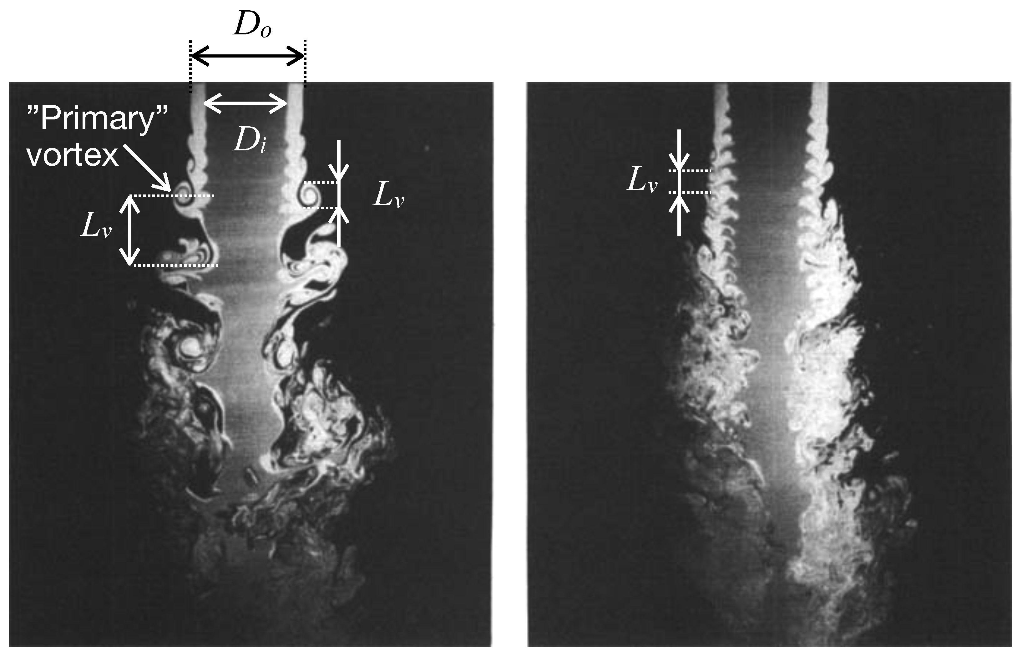
In contrast to a single steady, round jet (impinging on a smooth surface), little detailed, quantitative information is available on the vortex structure in the near-field of a coaxial (impinging) jet. Most of the available information comes from dye or smoke flow visualizations (e.g., Dahm et al. [15]) indicating that by either changing the velocity ratio or the absolute velocities while keeping the velocity ratio constant, the near-field flow dynamics can be manipulated. As is well-known, Kelvin–Helmholtz instabilities in the near-field flow generate toroidal (primary) vortices near the nozzle exit (Figure 2) that remain coherent for a short distance and then break-up into small-scale structures [18]. Note that recent experiments by Raizner et al. [19] showed that jet pulsation increased the primary vortex shedding frequency, leading to enhanced heat transfer at small stand-off distance, (= 2), where H denotes the distance between the jet exit and the impingement plate, and D is the jet diameter. As can be observed in the visualizations depicted in Figure 2, besides the effect of the velocity ratio, the spacing or size, , of the primary vortices also greatly depends on the magnitude of the absolute velocities. Since heat and mass transfer enhancement in the near-field of the impinging jet is associated with primary vortex properties, such as their strength and frequency, it may be anticipated that enhancement can be optimized by fine-tuning coaxial jet variables such as , the mass flow rate and pulsation frequency.
In this review, we will start by discussing free coaxial jets having a thin lip thickness in Section 2. First, the governing equations will be presented and the importance of the Reynolds shear stress distributions on the axial static pressure distribution is pointed out in Section 2.1. Next, the effect of the velocity, diameter and area ratios as well as the absolute values of the inner and outer jet exit velocities on the flow field and in particular on the governing instabilities is discussed in Section 2.2. In Section 3, the differences and similarities between using a blockage disk or a thick lip thickness are discussed. The lack of studies on impinging coaxial jets is illustrated by Section 4 that discusses the available literature on this subject. Finally, in Section 5, some applications of coaxial impinging jets that may lead to enhanced performance in the field of heat and mass transfer are discussed.
2. Free Coaxial Circular Jets
In this section, a survey of the relevant literature on free coaxial circular jets will be presented. First, the governing equations and importance of different terms are discussed in Section 2.1 after which the general flow field characteristics are reviewed in Section 2.2. Section 2.3 provides a summary and some conclusions that can be drawn based on the discussed literature results. We limit ourselves to coaxial jets flowing into a quiescent fluid of the same density.
2.1. Importance of Different Terms in the Governing Equations
In jet flows, the mean static pressure gradient in the direction of the flow is commonly neglected. However, static pressure measurements in a 2D turbulent slot jet by Miller and Comings [20] revealed appreciable deviations from this assumption and showed that they were associated with the local Reynolds stress distributions. More insight into the importance of the Reynolds stresses can be obtained by looking at the governing equations as will be done in the following.
Based on the Navier–Stokes equations and using Reynolds decomposition, the Reynolds averaged Navier–Stokes (RANS) equations can be derived, and for a non-swirling, statistically stationary, axi-symmetric jet, expressed in cylindrical coordinates (; see Figure 1), are given by [21]:
where and W denote the instantaneous axial, radial and azimuthal velocities (Figure 1), P denotes the instantaneous static pressure and the fluid density. An overbar denotes a time average and lower case velocity components denote the velocity fluctuations (Reynolds decomposed). The Laplace operator in cylindrical coordinates is denoted by . The RANS equations indicate that gradients of several Reynolds stress components may be of importance. Note that the viscous terms (the last terms on the right hand side of Equations (7) and (8) may be neglected for high Reynolds number turbulent flows.
The x-momentum equation (Equation (7)) can be rearranged (neglecting the viscous term) using the continuity equation, as follows:
In this form, it is observed that the first term within parenthesis contains the total pressure (i.e., dynamic plus static pressure) as well as the normal streamwise Reynolds stress component. This term is balanced by the right term in parentheses that contains the Reynolds shear stress. Similarly, the r-momentum equation (Equation (8)) can be rearranged as:
Invoking boundary layer approximations (, and “slenderness” of the mixing layer) and using the r-momentum equation, the x-momentum equation (Equation (9)) can be written as:
where is a dummy variable and the pressure in the free stream () is denoted as . Note that the axial stress gradient term (within square brackets) is usually neglected. However, Miller and Comings [20] showed that the static pressure and the normal Reynolds stresses, and , as well as their gradients were of the same order of magnitude, but of opposite sign. As a result, mean flow deceleration along a streamline almost entirely depends on the lateral gradient of the Reynolds shear stress, .
Miller and Comings [22] continued their investigation of force–momentum fields in a dual jet flow configuration having much more significant static pressure effects, and found that the acceleration of the mean flow in the positive x-direction in the near-field region is due to the lateral Reynolds shear stress gradient. The streamwise static pressure gradient alternately reinforced and opposed the mean flow acceleration, and flow stagnation occurred at the point where the two opposing forces equaled. Furthermore, they showed that the streamwise gradient of the normal Reynolds stress component, , was generally negligible compared to the static pressure and turbulent shear stress forces. A few decades later, in the near-field of a coaxial jet, Rehab et al. [16] used this balance of forces as the basis for modeling the onset of recirculation (Figure 1) at high . Based on their model, the critical velocity ratio representing the recirculation threshold was, , i.e., close to their experimentally found value of .
In conclusion, the force–momentum balance in the near-field of a coaxial jet is a balance between the mean, adverse static axial pressure gradient that tends to decelerate the flow and causes back flow towards the inner nozzle, and the radial Reynolds shear stress gradient which accelerates the flow in the positive x-direction against the static pressure gradient.
2.2. General Flow Field Characteristics
In this section, the general flow field characteristics of coaxial jets are reviewed and, in particular, the effect of the velocity and area ratios as well as the inner and outer jet Reynolds numbers on the initial flow field of a coaxial jet is discussed. Literature publications pertinent to this section are summarized in Table 1. Note that in this table only studies are shown in which the “lip” thickness of the inner jet nozzle, t (Figure 1), did not exceed 2 mm (considered small). The effect of increased “lip thickness” (or “blockage”) will be discussed in Section 3.
The first studies on coaxial axi-symmetric jets were performed in the 1940s [30,31,32] as summarized by Forstall and Shapiro [33]. Forstall and Shapiro [33] were interested in the mixing properties of the coaxial jet and they showed that the integral method analysis proposed by Squire and Trouncer [34] (circular jet issued into a co-flowing stream) using experimental constants, adequately predicted approximate values of concentration and velocity in the mixing region of the coaxial jet. However, Chigier and Beér [35] commented that the flow patterns in coaxial jets are sufficiently different from those considered by Squire and Trouncer [34] so that the effect of varying on the decay and spread of the inner jet is contrary to that predicted by Squire and Trouncer [34]. While mixing properties remained an important incentive for studying coaxial jets, later studies focused also on the similarities and differences in flow field characteristics between single circular jets and coaxial jets. For example, Champagne and Wygnanski [23] used hot wire anemometry to measure the radial profiles of mean velocities, turbulence intensities and shear stresses in coaxial turbulent air jets for two area ratios, = 2.94 and 1.28, and velocity ratios that ranged between (see Table 1). Their results indicated that far from the nozzle exit (), the coaxial jet becomes identical to a single axi-symmetric free jet and self-similarity is attained. In the developing region, close to the nozzle exit, their results indicated that the outer potential core length was more or less independent of and equaled about eight times the annular gap size, i.e., . In contrast, the inner core length not only decreased with increasing but also strongly depended on (see Figure 3 and associated discussion). When , low pressure in the inner core bends the outer jet inwards and this effect becomes stronger with decreasing , also shown by Rehab et al. [16].
2.2.1. Coaxial Jet Flow Structure
A large body of research on coaxial jets was accumulated in the 1970s and 1980s by Ko and co-workers [17,24,25,26,27]. These studies combined flow visualizations, hot wire measurements, mean pressure as well as fluctuating pressure measurements. Kwan and Ko [17] proposed a model based on their own as well as previous results in which they divided the flow field of the coaxial jet into three zones as depicted in Figure 1. The initial merging zone extends from the jet exit plane to the outer potential tip core, while the fully merged zone starts at the point where the inner and outer jets have fully merged and start to behave as a single jet. Note that based on available results, it takes some distance for the velocity profile in the fully merged zone to become fully developed and self-similar. The intermediate zone is more complicated and has properties intermediate to those of the previous described zones. Note that due to the velocity “jumps” between the inner and outer jet velocities, , inner and outer mixing layers (green and blue shaded areas in Figure 1) exist that give rise to Kelvin–Helmholtz instabilities that result in the generation of toroidal vortices close to the nozzle exit (Figure 2).
Furthermore, even when = 0 (i.e., when ), wake-like instabilities will form as a result of the finite lip thickness. Kwan and Ko [17] proposed a simple model that described the initial region of the developing coaxial jet as two separate arrays of non-interacting vortex rings originating in the inner and outer mixing layers. Their main model assumptions were: (i) the outer mixing layer is the result of a single jet of diameter and jet exit velocity shearing with the ambient fluid, and (ii) the inner mixing layer is the result of a single jet of diameter and jet exit velocity submerged in a uniform stream of velocity . In addition, Kwan and Ko [17] assumed that the fully merged zone is similar to that of an equivalent single jet of equal thrust. Based on this simple model, the average separation distance of consecutive inner and outer mixing layer vortices was estimated as 1.25 and 1.25, respectively, while inner mixing layer vortex convection velocities were estimated to be 0.6.
Ko and co-workers performed many experiments to validate their model. For example, Kwan and Ko [17] and Ko and Kwan [26] used hot wires and a microphone to study the initial merging region of coaxial jets for a range of velocity ratios, = 0.3, 0.5 and 0.7 (Table 1). Ko and Au [25] measured the velocity, pressure and their correlations for velocity ratios ranging between while keeping the outer jet velocity constant, = 50 m/s (Table 1). All specifically focused on self-similarity of the mean velocity and turbulence intensity profiles in the near field of the coaxial jet in comparison to single jets. They found that the radial distribution of the time-averaged, axial velocity of the outer jet exhibited fairly good similarity between , agreeing with single jet results reported by Bradshaw et al. [39] and Ko and Davies [40], amongst others. In addition, the inner jet behaved like a single jet emanating in a co-flowing ambient and showed self-similarity with single jet results between (within the initial merging zone). However, in the intermediate merging zone, self-similarity of the inner and outer jets was absent, only reappearing in the fully-merged zone for . Two dominant, low and high frequencies, were identified in the outer and inner mixing layers, respectively, strengthening their model assumption of two non-interacting vortex arrays.
Additionally, Ko and Au [25] detected the higher Strouhal number peak (associated with the inner mixing layer) mainly for in the range . In contrast, the lower Strouhal number peak (associated with the outer mixing layer) was detected for all investigated and was most pronounced when . Dominance of the high or low frequency in the power spectrum depended on , with the outer mixing layer becoming more dominant with increasing . Results that further strengthened the model of two separate, non-interacting vortex trains were provided by the measurements of Ko and Kwan [26] who focused on the covariances of pressure fluctuations and axial and radial velocity fluctuations. Measured pressure intensity spectra indicated that relative dominance of the inner and outer mixing layers depended on . For = 0.3, inner mixing layer vortices dominated, while for = 0.5, both inner and outer mixing layer vortices were important at small axial distances from the nozzle exit; for = 0.7, outer mixing layer vortices dominated. The main conclusion drawn by Ko and co-workers was that the complicated flow structure of coaxial jets can be understood and described by the much simpler structure of single jets. However, later studies such as the dye visualizations by Dahm et al. [15] and the work by Rehab et al. [16] have shown that this model is too simplified and depending on as well as t, the two mixing layers may interact in the immediate near-field of the coaxial jet (see also Chigier and Beér [35]).
2.2.2. Near-Field Flow and Instability Dynamics
The first high quality dye visualizations of the near-field flow structure of coaxial jets for a wide range of velocity ratios were performed by Dahm et al. [15] for relative low Reynolds numbers and a single area ratio (see Table 1). In agreement with previous studies, they showed that for a given nozzle geometry, the near-field flow characteristics were dictated by . However, they also showed that the absolute values of the jet exit velocities or alternatively, their respective Reynolds numbers, strongly affected the vortex generation in the near-field region of the coaxial jet (Figure 2). Their results indicated that the near-field flow characteristics are governed by competing wake and shear instabilities. The latter are the result of the velocity jump between the inner and the outer jet, (inner shear instabilities), and that between the outer jet and the quiescent surroundings, (outer shear instabilities). Wake-like instabilities are characterized by opposite sign vortices and are the result of the finite lip thickness (Figure 1). They become visible when the velocity ratio is close to unity and inner shear instabilities are weak. The results obtained by Dahm et al. [15] indicated that when 0.6, outer shear instabilities governed and inner shear layer instabilities were suppressed. Kelvin–Helmholtz instabilities led to the generation of toroidal vortices that were helical at = 0.59, but became axi-symmetric at = 0.71. In the former case, the inner surface deformed only in response to the helical vortical structures in the outer layer while in the latter case, the inner interface started to show signs of an instability and outer layer vortex pairing led to a quick collapse of the potential core of the inner jet as ambient fluid was brought into its core as a result of these pairings. In the range 0.9, the inner shear instability became important while also weak wake instabilities could be discerned. Note that for all values of , outer shear instabilities were present and ultimately governed the flow field downstream.
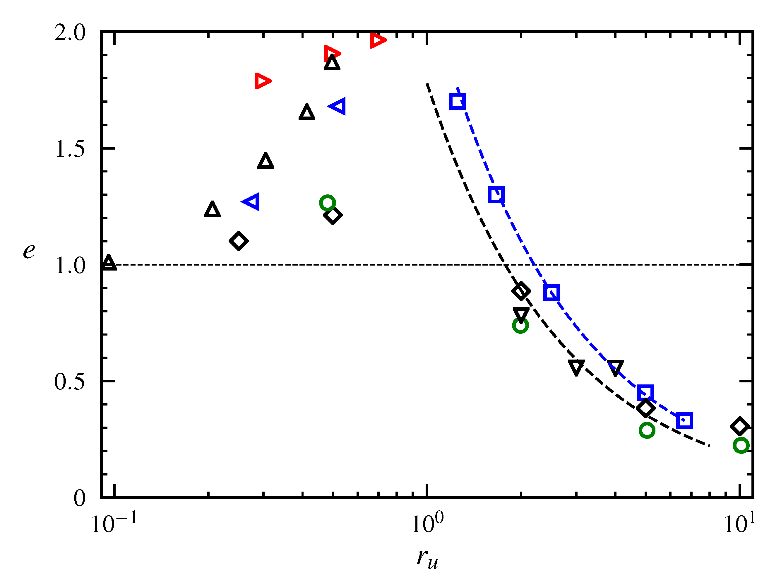
Au and Ko [27] defined the elongation, e, as the ratio between the inner potential core length with external (annular or co-flowing) flow to that without external flow. Their findings for e are compiled together with data from other literature sources and charted as a function of in Figure 3. The results indicate that the inner potential core of a coaxial jet exceeds that of a single jet when , while it is shorter when (). As mentioned before, the area ratio affects the inner potential core length, explaining some of the observed scatter in Figure 3, especially when .
A special situation occurs when , and the velocity jump across the inner mixing layer is small. In this case, the only acting instability besides the outer mixing layer instability, is the wake instability. However, as noted by Dahm et al. [15], wake instabilities only play a minor role in the overall flow dynamics ( 2 mm) since the outer shear layer instabilities remained dominant at their relative low Reynolds numbers. Increasing the Reynolds numbers (by increasing and ) led to increased importance of wake instabilities over shear instabilities due to the increased velocity defect [29]. As a result, increasing the Reynolds numbers (for a given nozzle geometry) profoundly changed the near-field flow characteristics (Figure 2). While Dahm et al. [15] showed this only for = 1.0, Reynolds number effects are also expected for other velocity ratios. Interestingly, the inner jet’s core region at = 1 exceeded that at = 0.71 (see also Figure 3), perhaps due to increased symmetry of the generated toroidal vortices. The nature of the shear instability depends on the velocity jump across the layer. Upon increasing the velocity ratio beyond , the inner to outer velocity jump changes sign and the inner shear instabilities become increasingly significant ( = 1.14 and 2.56). However, now the vortices generated in the inner and outer mixing layers interact and the two layers do not develop independently of each other as was assumed in the model proposed by Ko and Kwan [26]. Instead, disturbances generated by each layer affect each other and “locking” between the two shear layers is indicated by matching inner and outer vortex generation frequencies. As the two layers “lock on”, the core region is further shortened (see also Figure 3). As is increased beyond , flow recirculation is observed, in detail analyzed by Rehab et al. [16].
Wicker and Eaton [29] reported on instantaneous smoke visualizations of coaxial jet flow as a function of for a single nozzle exit area ratio. They also examined the effectiveness of applying single frequency acoustic forcing in controlling the near-field structure. Their flow visualizations indicated widely varying near-field vortex structure dynamics depending on similar as reported by Dahm et al. [15]. In their configuration, the inner and outer shear layers were separated by a relative large annular gap (see Table 1) and initial vortex development in the inner and outer mixing layers occurred independently. However, the outer layer, large-scale structures ultimately governed the inner flow. By applying acoustic excitation based on single jet shear instabilities, they were able to control the inner mixing layer structures’ wavelengths and sizes. However, inner jet axial excitation did not have much effect on the outer mixing layer. In contrast, outer jet excitation led to large scale outer mixing layer structures similar to those observed for a single jet and provided a strong coupling between inner and outer mixing layers.
Rehab et al. [16] investigated the near flow field structure of coaxial water jets having large velocity ratios, (Table 1). In all of these cases, the outer jet governed the near-field flow structure. Based on a force–momentum balance (Section 2.1, Miller and Comings [20]) and accompanying experiments, they showed that there exists a critical velocity ratio, , beyond which a recirculatory “bubble” appears at the end of the inner jet’s core region as a result of a strong adverse static pressure gradient (see also Figure 1). For moderate velocity ratios (), the inner potential core length, , varied as (see also Figure 3), with the numerical constant, A, ranging between 5 . Note that the exact value of A is mainly governed by the diameter ratio, , or alternatively, (for a given nozzle configuration). For example, raising (for a given ), increases the annular gap and as a result the outer potential core length increases. Therefore, the inner jet will be pinched off farther downstream leading to a longer inner jet potential core region. Increasing the Reynolds numbers (for a given nozzle geometry) while keeping constant [15] reduces the inner potential core length slightly. However, this Reynolds number effect appears to be weak compared to the effect of . As can be observed in Figure 3, the variation of e is well described by , where (= ) incorporates the inner potential core length of a single jet, , where the superscript “s” denotes “single”. Values of A are A = 8 and 9.9 for the data reported by Rehab et al. [16] (black dashed curve) and Au and Ko [27] (blue dashed curve), respectively.
Further note that the nozzle geometry of coaxial jets and the resulting initial flow conditions (fully developed pipe flows or uniform, top hat velocity profiles, Table 1) does not alter the inner potential core variation law (), although it changes the value of A. Sadr and Klewicki [14] investigated the development of turbulence characteristics in the near-field of coaxial jets using molecular tagging velocimetry (MTV) at velocity ratios smaller than and close to (Table 1). Jet exit profiles were those of a fully developed turbulent velocity profile of the center jet and a top hat profile of the annular jet. This combination reduced the inner layer’s shear resulting in a longer inner core length. Their results mostly confirmed previous results especially regarding the reduction of the potential core length with increasing . Not much new insight into the generation of the near-field vortices was provided and the results mainly reported on the development of the turbulence characteristics such as turbulence intensities, turbulent kinetic energy production, Taylor microscale, amongst others.
2.3. Discussion
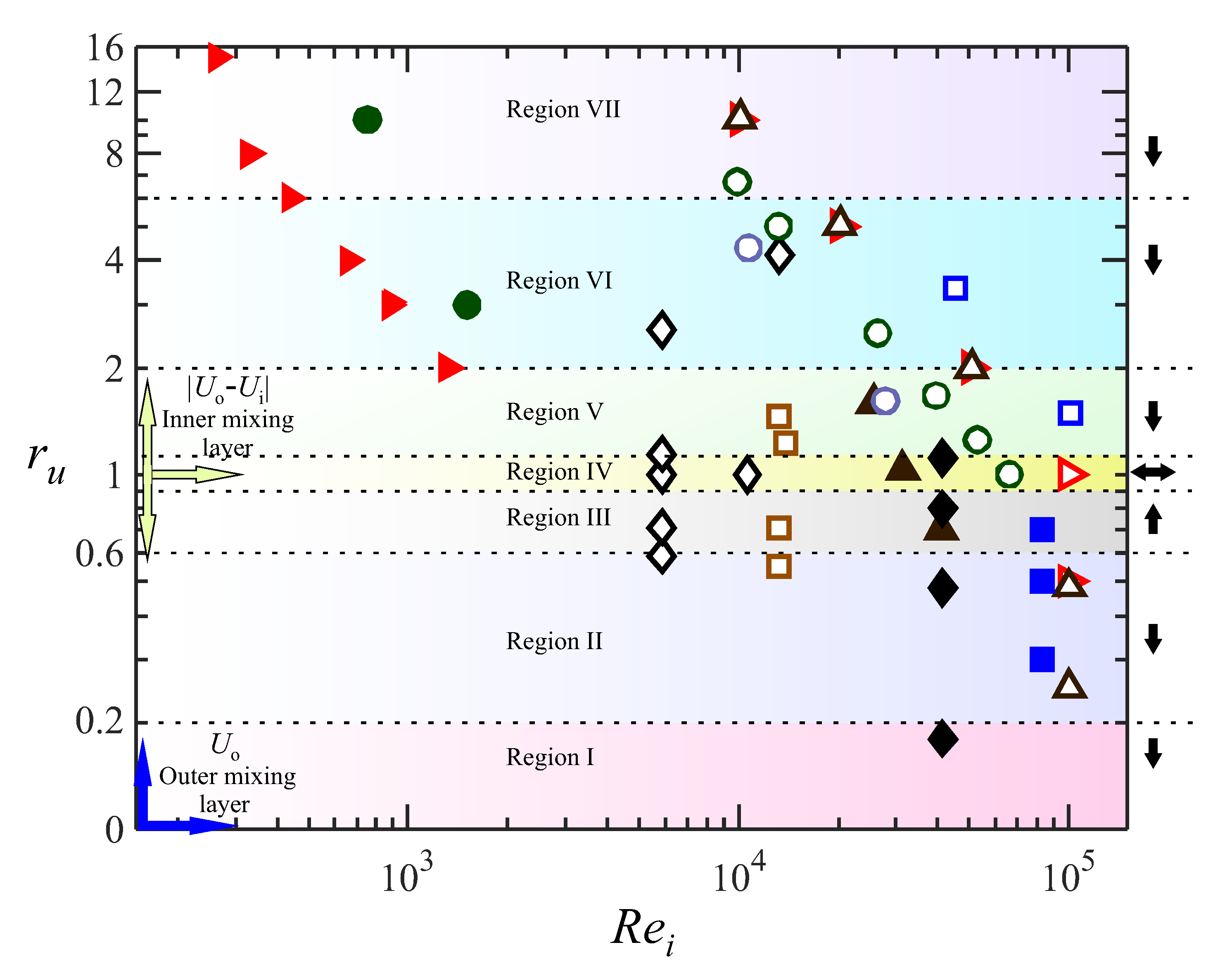
Based on the available literature data, information on the dominant instabilities can be extracted and different regions can be defined according to based on the relative importance of inner mixing layer wake or shear instabilities denoted by and , respectively. Note that shear instabilities in the outer mixing layer are always present for coaxial jet flow into quiescent surroundings. The different identified regions are summarized in Table 2 according to ranges. However, note that the identified bounds incorporate a relatively large uncertainty due to the limited availability of data. Region I consists of 0.2, where wake instabilities are absent and shear layer instabilities are “very strong” as a result of the large magnitude of the inner mixing layer’s velocity jump, . In region II (, decreases but still remains strong. In region III, defined by , the first signs of weak wake instability are observed, however, remains dominant. This changes in region IV (), where weakens and is strong and governs. In region V (), wake instabilities again weaken and is dominant. In regions VI and VII, for even larger , becomes negligible while is dominant. In these regions (), “locking” between the inner and outer mixing layer vortices occurs and becomes increasingly strong with increasing . In addition to Table 2, the relevant literature investigations and the different region boundaries (dashed lines) are presented in Figure 4 as versus Re.
Although Reynolds number effects seem to be important, their specific role is unclear due to a lack of data. Therefore, in Figure 4 the ranges are separated by horizontal dashed lines of constant . Yellow and blue arrows depicted in Figure 4 point in the direction of increasing magnitudes of inner and outer mixing layer velocity jumps, and , respectively. Black arrows associated with each identified region point into the direction of increasing inner potential core length. In general, wake instabilities are only important when 1, and weaken when departs from unity. For low , Region I, Table 2 and Figure 4), the inner jet dominates the outer one with high shear at the inner mixing layer and the inner potential core exceeds that of a single jet [26]. For (Region II, Table 2 and Figure 4), outer shear instabilities govern while wake and shear instabilities in the inner mixing layer are negligible. As is increased to (Region III, Table 2 and Figure 4), wake instabilities appear. These are in general weak, especially at the low Reynolds numbers investigated by Dahm et al. [15].
However, they are expected to become increasingly significant as Re is increased while keeping constant as shown by Dahm et al. [15] (Figure 2). For , the velocity jump across the inner mixing layer is small and wake instabilities govern the flow field while inner shear instabilities are weak. Upon increasing the velocity ratio to values exceeding (regions V, VI and VII), the inner mixing layer velocity jump, , changes sign and inner shear instabilities become equally important as the outer mixing layer ones. In these regions, inner and outer mixing layer vortices strongly interact, and their shedding frequencies lock on to each other. As is increased beyond > 6 − 8 (Region VII, Table 2 and Figure 4), a recirculation region forms [16] that shortens the potential core length. It should be noted that for a given , increasing the absolute values increases the inner and outer velocity jumps and the relative importance of the different instabilities may change. As a result, we anticipate different flow field dynamics with increasing Reynolds numbers, a topic that has hardly been investigated.
3. Some Remarks on Geometrical Nozzle Modification
It is not within the scope of this review article to discuss all possible geometrical nozzle modifications. Instead we focus here on the effect of increasing the lip thickness by either increasing the inner nozzle’s wall thickness (Figure 5a) or by placing a blockage disk (Figure 5b). These modifications will affect the wake and shear instabilities and their relative strength.
In case of a blockage disk, the blockage ratio is defined as the ratio between the “blocked” area (including the inner jet) and the total area of the outer jet, (Figure 5b). In a similar manner, it can be defined for an aerodynamically shaped nozzle as, (Figure 5a). An overview of relevant literature publications is presented in Table 3. Note that for a sharp lip (small t) of the inner nozzle, the recirculation region in the wake of the lip will be negligible (see Figure 1). However, increasing the lip thickness, or placing a blockage disk, results in an appreciable recirculation zone just downstream of it. This axi-symmetric (toroidal) recirculation zone is formed to satisfy the entrainment requirements of both the inner and the outer jets [35]. The effect of increasing t for an aerodynamically shaped nozzle (Figure 5a) has been investigated by Buresti et al. [41] and Segalini and Talamelli [46] who showed that a thick inner nozzle lip ( mm) enhanced the mixing of the inner and outer jets when . Vortex shedding was characterized by a Strouhal number of based on t and . Flow visualizations by Segalini and Talamelli [46] clearly showed the presence of an axi-symmetric “von Kármán vortex street” in the inner mixing layer, indicating that wake instability dictated mixing dynamics for velocity ratios close to unity.
Figure 6 and Figure 7 depict the streamline patterns observed downstream of an aerodynamically shaped nozzle and one with a blockage disk installed. Note that the blockage ratios were similar in all cases and in particular the effect of changing is seen. For annular flow (, Figure 6a), a toroidal vortex (TV, in the cross section of Figure 6a indicated as a counter rotating pair of vortices) appears in the initial merging zone (or recirculation zone) of the annular jet for the aerodynamically shaped nozzle. However, upon introducing the inner jet and as a result of the inner velocity jump, , the streamline pattern changes and now a pair of counter-rotating toroidal vortices (TV and TV), a stagnation point (SP) at the center line and an off-axis stagnation “circle” (SC, Figure 6) can be observed.
It is interesting to compare the streamlines pattern obtained for an aerodynamically shaped nozzle (Figure 6b) to that with a blockage disk installed (Figure 7a), while keeping and constant but with significantly different Reynolds numbers (Table 3). Despite the similarity in the appearance of the pair of counter-rotating toroidal vortices, the overall topology changed. In particular, the off-axis stagnation “circle” observed for the aerodynamically shaped nozzle (Figure 6b) converged to the center line for the nozzle when the blockage disk was installed (Figure 7a). In addition, in the latter configuration, the flow field exhibits reverse flow between two centerline stagnation points (SP and SP). Note that besides the different nozzle geometry, Reynolds numbers differed by several orders of magnitude which likely had an effect on the streamline patterns. When decreasing while keeping nearly constant (blockage disk installed, Figure 7), the centerline stagnation points disappear and no reverse flow is observed at the centerline (Figure 7b). Note that, in addition to the above described similarities and differences in the streamline patterns for the two presented nozzle geometries, having a blockage disk installed leads to a significant radial velocity component at the nozzle exit, creating a larger toroidal vortex associated with the outer layer in the initial merging zone.
4. Coaxial Circular Jets Impinging on a Flat, Smooth Surface
While there is quite some information on the flow field characteristics in the near-field of coaxial jets (as discussed in Section 2 and Section 3), impinging coaxial jets have barely been studied [6,7,49,50,51,52]. This is surprising in light of the expected potential for enhancing heat and mass transfer especially for impingement at relatively small stand-off distances (). At these stand-off distances, the coaxial jet does not act as a single jet and more importantly the near-field flow characteristics can be changed by varying the velocity ratio (see Section 2.2). It is well known that heat and mass transfer in impinging jet flows (at small ) is closely associated with the vortices generated in the near-field by Kelvin–Helmholtz instabilities [53,54]. Impingement of these “primary” vortices and the subsequent generation of “secondary” ones is thought to be reason for the observed Nusselt number peak slightly away from the stagnation point (e.g., [55,56]). Since coaxial jets exhibit especially complex vortex generation and interaction mechanisms, their usage enables to fine-tune between heat and mass transfer needs and the coaxial jet flow characteristics. However, the few published literature studies all focus on the heat transfer characteristics and mainly report radial profiles of average Nusselt numbers and how these are affected by changing the stand-off distance and the nozzle configuration. Available flow field information of impinging coaxial jets lacks details on the instantaneous vortex dynamics in the near-field that is essential for the understanding of this complex convective heat transfer problem. Flow field and heat transfer characteristics of publications pertinent to impinging coaxial jets are summarized in Table 4 and Table 5, respectively.
Celik and Eren [7] performed measurements and compared between the radial distribution of the average Nusselt number for a single circular impinging jet and that for a coaxial jet. As is well-known, for a single circular jet impinging onto a flat, smooth surface, the radial distribution of the mean Nu-number decreases away from the stagnation point and for small stand-off distances exhibits a secondary local maximum slightly away from the stagnation point. The latter is associated with the impingement of primary vortices and the generation of secondary ones, leading to periodic destruction and restablishment of the boundary layers. Similar results have been obtained for coaxial jets. However, in this case the picture is more complex since for a given total mass flow rate, the ratio between the outer and total mass flow rate, , changes the Nu number distribution significantly [6], and increasing leads to a more uniform radial Nu-number distribution. As a result, high values of are preferred for cooling a large surface area while low can be used for more localized cooling demands. It is interesting to point out that the stagnation point Nu-number decreases with increasing while the area averaged Nu-number increases with increasing . As in the case for a single impinging jet, also for coaxial jets, the area averaged Nu-number decreases with increasing .
Celik and Eren [7] performed flow velocity measurements using hot-wire anemometry and reported radial profiles of the mean axial jet velocity and corresponding turbulence intensities for different and . Terekhov et al. [51] measured the flow field and heat transfer in an impinging annular jet and in agreement with Celik and Eren [7] also found that for the same mass flow rate, the annular jet’s heat transfer was enhanced compared to that of a single round jet having the same diameter as the outer annulus. The absolute value of the enhancement depended on the annular gap size and . They performed particle image velocimetry (PIV) measurements, but besides two instantaneous velocity maps, only mean velocities and rms distributions were presented, and no detailed investigation of the underlying physical mechanism of the reported enhancement was presented.
The effect of the stand-off distance on the stagnation point Nu-number is well documented for a single jet (e.g., [58,59]). Results indicate that the stagnation point Nu-number peaks at , i.e., at the end of potential core region where the turbulent kinetic energy is highest, see also [60]. In contrast, for coaxial jets not many data have been published but all available data sets do not indicate a local maximum at a certain stand-off distance. Instead, all report on decreasing stagnation point Nu-numbers with increasing (up to = 12) [6,7,52], most likely due to the lack of potential core regions since all the reported coaxial nozzle configurations had fully developed turbulent jet exit profiles.
Changing the nozzle geometry is one of the most simple ways of changing the near-field flow dynamics of the coaxial jet (see also Section 3). In particular the effect of adding swirl (i.e., an azimuthal velocity component) to the jet flow has been investigated in the past for coaxial jets. Adding swirl increases the heat transfer coefficients and leads to a more uniform radial distribution of the average Nusselt numbers. For example, Markal [49,61] studied coaxial, confined turbulent impinging air jets and showed that by adding swirl to the outer annular jet, not only the spatial uniformity of Nu was enhanced, but also average Nu-numbers increased (compared to those of a steady jet at the same Re). Furthermore, local Nu-numbers decreased with increasing , while they increased with increasing total flow rate. They focused on Nusselt number distributions and pressure distributions, and no detailed flow field information was provided. Markal et al. [52] investigated the effect of modifying the annular jet geometry from a straight to a conical annular outlet. They concluded that cooling performance at close range impingement () was best for a cone angle of 20. Decreasing led to increasing local Nu-numbers. Furthermore, both the rate and spatial uniformity of the convective heat transfer strongly depended on the coupling between and the cone angle.
Due to the complex flow dynamics of impinging coaxial jets, only few numerical studies have been published [50,62]. Bijarchi and Kowsary [62] used the finite volume method to solve the Navier–Stokes equations and the energy equation for a laminar axi-symmetric, steady flow. Their aim was to achieve uniform heat transfer coefficients by inverse optimization. A recent numerical simulation based on the RANS equations [50], studying both the effects of center jet swirl as well as annular jet swirl, reached the same conclusions as those by Markal [49]. However, they mentioned that heat transfer may either be enhanced or reduced depending on the combination of the problem parameters.
The two main conclusions that can be drawn from the few published literature results on impinging coaxial jets are the following: (i) heat transfer is more effective for a coaxial jet than for a single jet at the same total mass flow rate [7], and (ii) overall heat transfer reduces with increasing . In short, there is a need for detailed investigations of the instantaneous flow field and heat transfer dynamics in impinging coaxial jets to elucidate the underlying physical phenomena that govern this complex convective heat transfer problem.
5. Some Practical Applications and Open Questions
In this section, some practical applications of impinging coaxial jets in mass and heat transfer are discussed as well as the remaining open questions.
5.1. Mass Transfer
As discussed in the previous sections, the coaxial jet’s near field flow structure may be modified to fine-tune flow time scales to those of dispersed particles thereby changing the Stokes number that governs the particle response to changes in the flow. One of the possible applications could be to control the orientation of deposited non-spherical particles such as fibers in order to create surfaces that have predefined, desired mechanical and optical properties. The response of a fiber (considered a proto-typical non-spherical particle) to changes in the flow is characterized by the Stokes number, defined as the ratio between the fiber response time, , and a suitable flow time scale, St = . The fiber’s translational response time for randomly oriented fibers in Stokes flow, depends on the aspect ratio, , and is given by [63,64]:
where d is the fiber diameter, L its length, the material fiber density and the fluid dynamic viscosity. Thus, for given , and , strongly depends on d. Note that the fiber’s rotational response time is smaller than the translational one [65].
The choice of the relevant flow time scale, , in a coaxial jet is non-trivial due to the complexity of the flow field, and in the available literature different definitions have been used [66,67,68]. The proper flow time scale will depend on the distance from the nozzle. In the jet’s near field (up to ∼), it may be defined as, [69], where denotes a length scale associated with the generated primary vortices such as their diameter or spacing (see Figure 2, [69]), and is their convection velocity; in the inner mixing layer and in the outer one.
Note that the coaxial jet has the advantage that the inner jet’s exit conditions can be kept constant while the inner mixing layer characteristics and can be manipulated by changing . As a result, for constant inlet conditions of the inner jet, one can study fiber interaction with the inner mixing region structures for a wide range of Stokes numbers. Note that the same is valid while keeping constant and changing . As a result, the coaxial jet provides a highly versatile system to study the interaction of non-spherical particles with vortical structures and its possible application to the fabrication of “high-tech” surfaces by controlled particle deposition.
5.2. Heat Transfer
As mentioned in this review, the heat transfer characteristics of single, circular impinging jets have been studied extensively and a typical observation is that the Nu-number distribution displays a secondary, local maximum slightly away from the stagnation point (see Hadžiabdić and Hanjalić [56] and references herein). The convective heat transfer characteristics are strongly coupled with the flow field and this secondary local maximum appears to coincide with the impingement of large scale, primary vortices that generate secondary vortices [56,70] at relatively small stand-off distances. However, there is a lack of combined, detailed flow and heat transfer studies to further elucidate the governing physical mechanisms.
A promising method to enhance heat transfer is using a pulsating impinging jet (at constant average mass flow rate) [4,5,71] that causes intermittent break-up and renewal of the hydrodynamic and thermal boundary layers [3,4,72,73,74]. However, depending on the pulsation frequency and amplitude, both enhanced and reduced time-averaged heat transfer coefficients have been reported [4,72]. For example, using time-resolved planar PIV measurements in conjunction with heat transfer and shear stress measurements, Janetzke et al. [72] and Janetzke and Nitsche [4] showed that jet pulsation resulted in boundary layer renewal. Overall heat transfer enhancement up to 20% was obtained at the stagnation point. Based on flow visualizations and heat transfer measurements, Liu and Sullivan [3] concluded that stagnation point heat transfer enhancement or reduction of a pulsating impinging jet was associated with the development of primary-secondary vortex pairs in the wall jet.
Despite several published results on pulsating impinging jets accumulated over the past two decades, the governing physical mechanisms remain largely unclear and many questions still remain unanswered regarding the effect of pulsation frequency, amplitude as well as the optimization of the impinging jet configuration. In addition, the practical implementation and control need further analysis. Furthermore, while steady coaxial jets have been shown to improve heat transfer compared to a single round jet having the same mass flow rate (see previous section), pulsating coaxial jets have not been studied. Some of the basic questions regarding coaxial impinging jets that still need to be answered are: (i) “What area ratio between the inner and outer jet leads to optimal heat removal?”, (ii) “What pulsation frequency optimizes heat removal?” and (iii) “What are the fundamental flow mechanisms responsible for heat transfer enhancement or attenuation?”.
Author Contributions
This review article was initiated by R.v.H. who prepared the first draft. The review is based on discussions between all four authors. In-depth analysis, adaptation and review have been done by R.v.H., S.M. and A.M.; B.C. was involved in the writing, review and editing of the manuscript. All authors have read and agreed to the published version of the manuscript.
Funding
This research was partially supported by the Pazy Foundation and the Israel Science Foundation (ISF) under grant number 2199/19.
Institutional Review Board Statement
Not applicable.
Informed Consent Statement
Not applicable.
Data Availability Statement
Data sharing not applicable.
Conflicts of Interest
The authors declare no conflict of interest.
References
- Kieffer, S.W.; Sturtevant, B. Laboratory studies of volcanic jets. J. Geophys. Res. Solid Earth 1984, 89, 8253–8268. [Google Scholar] [CrossRef] [Green Version]
- Camci, C.; Herr, F. Forced convection heat transfer enhancement using a self-oscillating impinging planar jet. J. Heat Transf. 2002, 124, 770–782. [Google Scholar] [CrossRef]
- Liu, T.; Sullivan, J. Heat transfer and flow structures in an excited circular impinging jet. Int. J. Heat Mass Transf. 1996, 39, 3695–3706. [Google Scholar] [CrossRef]
- Janetzke, T.; Nitsche, W. Time resolved investigations on flow field and quasi wall shear stress of an impingement configuration with pulsating jets by means of high speed PIV and a surface hot wire array. Int. J. Heat Fluid Flow 2009, 30, 877–885. [Google Scholar] [CrossRef]
- Hofmann, H.M.; Movileanu, D.L.; Kind, M.; Martin, H. Influence of a pulsation on heat transfer and flow structure in submerged impinging jets. Int. J. Heat Mass Transf. 2007, 50, 3638–3648. [Google Scholar] [CrossRef]
- Markal, B.; Aydin, O. Experimental Investigation of Coaxial Impinging Air Jets. Appl. Therm. Eng. 2018. [Google Scholar] [CrossRef]
- Celik, N.; Eren, H. Heat transfer due to impinging co-axial jets and the jets’ fluid flow characteristics. Exp. Therm. Fluid Sci. 2009, 33, 715–727. [Google Scholar] [CrossRef]
- Yule, A.J. Large-scale structure in the mixing layer of a round jet. J. Fluid Mech. 1978, 89, 413–432. [Google Scholar] [CrossRef]
- Geers, L.F.G.; Tummers, M.J.; Hanjalić, K. Experimental investigation of impinging jet arrays. Exp. Fluids 2004, 36, 946–958. [Google Scholar] [CrossRef]
- Banyassady, R.; Piomelli, U. Interaction of inner and outer layers in plane and radial wall jets. J. Turbul. 2015, 16, 460–483. [Google Scholar] [CrossRef]
- Zuckerman, N.; Lior, N. Radial Slot Jet Impingement Flow and Heat Transfer on a Cylindrical Target. J. Thermophys. Heat Transf. 2007, 21, 548–561. [Google Scholar] [CrossRef]
- Hoogendoorn, C. The effect of turbulence on heat transfer at a stagnation point. Int. J. Heat Mass Transf. 1977, 20, 1333–1338. [Google Scholar] [CrossRef]
- Lee, J. The Effect of Nozzle Configuration on Stagnation Region Heat Transfer Enhancement of Axisymmetric Jet Impingement. Int. J. Heat Mass Transf. 2000, 43, 3497–3509. [Google Scholar] [CrossRef]
- Sadr, R.; Klewicki, J.C. An experimental investigation of the near-field flow development in coaxial jets. Phys. Fluids 2003, 15, 1233–1246. [Google Scholar] [CrossRef]
- Dahm, W.J.A.; Frieler, C.E.; Tryggvason, G. Vortex structure and dynamics in the near field of a coaxial jet. J. Fluid Mech. 1992, 241, 371–402. [Google Scholar] [CrossRef]
- Rehab, H.; Villermaux, E.; Hopfinger, E. Flow regimes of large-velocity-ratio coaxial jets. J. Fluid Mech. 1997, 345, 357–381. [Google Scholar] [CrossRef]
- Kwan, A.; Ko, N. Coherent structures in subsonic coaxial jets. J. Sound Vib. 1976, 48, 203–219. [Google Scholar] [CrossRef]
- Violato, D.; Scarano, F. Three-dimensional evolution of flow structures in transitional circular and chevron jets. Phys. Fluids 2011, 23, 124104. [Google Scholar] [CrossRef] [Green Version]
- Raizner, M.; Rinsky, V.; Grossman, G.; van Hout, R. Heat transfer and flow field measurements of a pulsating jet impinging on a flat heated surface. Int. J. Heat Fluid Flow 2019, 77, 278–287. [Google Scholar] [CrossRef]
- Miller, D.R.; Comings, E.W. Static pressure distribution in the free turbulent jet. J. Fluid Mech. 1957, 3, 1–16. [Google Scholar] [CrossRef]
- Pope, S.B. Turbulent Flows; Cambridge University Press: Cambridge, UK, 2000. [Google Scholar]
- Miller, D.R.; Comings, E.W. Force-momentum fields in a dual-jet flow. J. Fluid Mech. 1960, 7, 237–256. [Google Scholar] [CrossRef]
- Champagne, F.; Wygnanski, I.J. An experimental investigation of coaxial turbulent jets. Int. J. Heat Mass Transf. 1971, 14, 1445–1464. [Google Scholar] [CrossRef]
- Ko, N.; Au, H. Initial region of subsonic coaxial jets of high mean-velocity ratio. J. Fluids Eng. 1981, 103, 335–338. [Google Scholar] [CrossRef]
- Ko, N.; Au, H. Coaxial jets of different mean velocity ratios. J. Sound Vib. 1985, 100, 211–232. [Google Scholar] [CrossRef]
- Ko, N.; Kwan, A. The initial region of subsonic coaxial jets. J. Fluid Mech. 1976, 73, 305–332. [Google Scholar] [CrossRef]
- Au, H.; Ko, N. Coaxial jets of different mean velocity ratios, part 2. J. Sound Vib. 1987, 116, 427–443. [Google Scholar] [CrossRef]
- Villermaux, E.; Rehab, H.; Hopfinger, E.J. Breakup régimes and self-sustained pulsations in coaxial jets. Meccanica 1994, 29, 393–401. [Google Scholar] [CrossRef]
- Wicker, R.B.; Eaton, J.K. Near field of a coaxial jet with and without axial excitation. AIAA J. 1994, 32, 542–546. [Google Scholar] [CrossRef]
- Victorin, K. Untersuchung turbulenter Mischvorgange. Forsch. Geb. Ing. A 1941, 12, 16. [Google Scholar] [CrossRef]
- Ribner, H.S. Field of Flow about a Jet and Effect of Jets on Stability of Jet-Propelled Airplanes; Technical Report; National Aeronautics And Space Admin Langley Research Center: Hampton, VA, USA, 1946. [Google Scholar]
- Deodati, J.B.; Monteath, E.B. An Investigation of the Round Jet in a Moving Air Stream. Ph.D. Thesis, California Institute of Technology, Pasadena, CA, USA, 1947. [Google Scholar]
- Forstall, W.J.; Shapiro, A. Momentum and Mass Transfer in Coaxial Gas Jets. J. Appl. Mech. 1950, 17, 399–408. [Google Scholar] [CrossRef]
- Squire, H.B.; Trouncer, J. Round Jets in a General Stream; Technical Report; Aeronautical Research Council: London, UK, 1944. [Google Scholar]
- Chigier, N.A.; Beér, J.M. The Flow Region Near the Nozzle in Double Concentric Jets. J. Basic Eng. 1964, 86, 797–804. [Google Scholar] [CrossRef]
- Kwan, S.-H. Noise Mechanisms in the Initial Region of Coaxial Jets. PhD. Thesis, University of Hong Kong, Hong Kong, China, 1975. [Google Scholar]
- Morris, P.J. Turbulence measurements in subsonic and supersonic axisymmetric jets in a parallel stream. AIAA J. 1976, 14, 1468–1475. [Google Scholar] [CrossRef]
- Rajaratnam, N. Developments in Water Science. In Turbulent Jets; Chow, V.T., Ed.; Elsevier: Amsterdam, The Netherlands, 1976; Volume 5. [Google Scholar]
- Bradshaw, P.; Ferriss, D.; Johnson, R. Turbulence in the noise-producing region of a circular jet. J. Fluid Mech. 1964, 19, 591–624. [Google Scholar] [CrossRef]
- Ko, N.; Davies, P. The near field within the potential cone of subsonic cold jets. J. Fluid Mech. 1971, 19, 49–78. [Google Scholar] [CrossRef]
- Buresti, G.; Talamelli, A.; Petagna, P. Experimental characterization of the velocity field of a coaxial jet configuration. Exp. Therm. Fluid Sci. 1994, 9, 135–146. [Google Scholar] [CrossRef]
- Buresti, G.; Petagna, P.; Talamelli, A. Experimental investigation on the turbulent near-field of coaxial jets. Exp. Therm. Fluid Sci. 1998, 17, 18–26. [Google Scholar] [CrossRef]
- Ribeiro, M.; Whitelaw, J. Coaxial jets with and without swirl. J. Fluid Mech. 1980, 96, 769–795. [Google Scholar] [CrossRef]
- Duraõ, D.; Whitelaw, J. Turbulent mixing in the developing region of coaxial jets. J. Fluids Eng. 1973. [Google Scholar] [CrossRef]
- Murugan, S.; Huang, R.F.; Hsu, C.M. Time-averaged flow characteristics and mixing properties of double-concentric jets. Int. J. Heat Fluid Flow 2020, 86, 108707. [Google Scholar] [CrossRef]
- Segalini, A.; Talamelli, A. Experimental analysis of dominant instabilities in coaxial jets. Phys. Fluids 2011, 23, 024103. [Google Scholar] [CrossRef]
- Huang, R.; Lin, C. Flow characteristics and shear-layer vortex shedding of double concentric jets. AIAA J. 1997, 35, 887–892. [Google Scholar] [CrossRef]
- Huang, R.F.; Lin, C.L. Visualized flow patterns of double concentric jets at low annulus velocities. AIAA J. 1994, 32, 1868–1874. [Google Scholar] [CrossRef]
- Markal, B. Experimental investigation of heat transfer characteristics and wall pressure distribution of swirling coaxial confined impinging air jets. Int. J. Heat Mass Transf. 2018, 124, 517–532. [Google Scholar] [CrossRef]
- Afroz, F.; Sharif, M.A.R. Heat Transfer from a Heated Flat Surface Due to Swirling Coaxial Turbulent Jet Impingement. J. Therm. Sci. Eng. Appl. 2020, 1–26. [Google Scholar] [CrossRef]
- Terekhov, V.; Kalinina, S.; Sharov, K. An experimental investigation of flow structure and heat transfer in an impinging annular jet. Int. Commun. Heat Mass Transf. 2016, 79, 89–97. [Google Scholar] [CrossRef]
- Markal, B.; Avci, M.; Aydin, O. Conical coaxial impinging air jets: Angle effect on the heat transfer performance. Heat Mass Transf. 2020, 1–12. [Google Scholar] [CrossRef]
- van Hout, R.; Rinsky, V.; Grobman, Y.G. Experimental study of a round jet impinging on a flat surface: Flow field and vortex characteristics in the wall jet. Int. J. Heat Fluid Flow 2018, 70, 41–58. [Google Scholar] [CrossRef]
- Raizner, M.; Rinsky, V.; Grossman, G.; van Hout, R. Effect of impinging jet pulsation on primary and secondary vortex characteristics. Int. J. Heat Mass Transf. 2020, 151, 119445. [Google Scholar] [CrossRef]
- Garimella, S.V.; Rice, R. Confined and submerged liquid jet impingement heat transfer. J. Heat Transf. 1995, 117, 871–877. [Google Scholar] [CrossRef]
- Hadžiabdić, M.; Hanjalić, K. Vortical structures and heat transfer in a round impinging jet. J. Fluid Mech. 2008, 596, 221–260. [Google Scholar] [CrossRef]
- Celik, N. Effects of the surface roughness on heat transfer of perpendicularly impinging co-axial jet. Heat Mass Transf. 2011, 47, 1209–1217. [Google Scholar] [CrossRef]
- Baughn, J.; Shimizu, S. Heat transfer measurements from a surface with uniform heat flux and an impinging jet. J. Heat Transf. 1989, 111. [Google Scholar] [CrossRef]
- Behnia, M.; Parneix, S.; Durbin, P.A. Prediction of heat transfer in an axisymmetric turbulent jet impinging on a flat plate. Int. J. Heat Mass Transf. 1998, 41, 1845–1855. [Google Scholar] [CrossRef]
- Kataoka, K.; Suguro, M.; Degawa, H.; Maruo, K.; Mihata, I. The effect of surface renewal due to largescale eddies on jet impingement heat transfer. Int. J. Heat Mass Transf. 1987, 30, 559–567. [Google Scholar] [CrossRef]
- Markal, B. The effect of Total flow rate on the cooling performance of swirling coaxial impinging jets. Heat Mass Transf. 2019, 55, 3275–3288. [Google Scholar] [CrossRef]
- Bijarchi, M.A.; Kowsary, F. Inverse optimization design of an impinging co-axial jet in order to achieve heat flux uniformity over the target object. Appl. Therm. Eng. 2018, 132, 128–139. [Google Scholar] [CrossRef]
- Shapiro, M.; Goldenberg, M. Deposition of glass fiber particles from turbulent air flow in a pipe. J. Aerosol Sci. 1993, 24, 65–87. [Google Scholar] [CrossRef]
- Zhang, H.; Ahmadi, G.; Fan, F.G.; McLaughlin, J.B. Ellipsoidal particles transport and deposition in turbulent channel flows. Int. J. Multiph. Flow 2001, 27, 971–1009. [Google Scholar] [CrossRef]
- Voth, G.A.; Soldati, A. Anisotropic particles in turbulence. Annu. Rev. Fluid Mech. 2017, 49, 249–276. [Google Scholar] [CrossRef] [Green Version]
- Sadr, R.; Klewicki, J.C. Flow field characteristics in the near field region of particle-laden coaxial jets. Exp. Fluids 2005, 39, 885–894. [Google Scholar] [CrossRef]
- Fang, C.; Xu, J.; Zhao, H.; Li, W.; Liu, H. Experimental investigation on particle entrainment behaviors near a nozzle in gas–particle coaxial jets. Powder Technol. 2015, 286, 55–63. [Google Scholar] [CrossRef]
- Lin, J.; Shi, X.; Yu, Z. The motion of fibers in an evolving mixing layer. Int. J. Multiph. Flow 2003, 8, 1355–1372. [Google Scholar] [CrossRef]
- Longmire, E.K.; Eaton, J.K. Structure of a particle-laden round jet. J. Fluid Mech. 1992, 236, 217–257. [Google Scholar] [CrossRef]
- Violato, D.; Ianiro, A.; Cardone, G.; Scarano, F. Three-dimensional vortex dynamics and convective heat transfer in circular and chevron impinging jets. Int. J. Heat Fluid Flow 2012, 37, 22–36. [Google Scholar] [CrossRef]
- Mladin, E.; Zumbrunnen, D. Local convective heat transfer to submerged pulsating jets. Int. J. Heat Mass Transf. 1997, 40, 3305–3321. [Google Scholar] [CrossRef]
- Janetzke, T.; Nitsche, W.; Täge, J. Experimental investigations of flow field and heat transfer characteristics due to periodically pulsating impinging air jets. Heat Mass Transf. 2008, 45, 193–206. [Google Scholar] [CrossRef]
- Xu, P.; Yu, B.; Qiu, S.; Poh, H.J.; Mujumdar, A.S. Turbulent impinging jet heat transfer enhancement due to intermittent pulsation. Int. J. Therm. Sci. 2010, 49, 1247–1252. [Google Scholar] [CrossRef]
- Xu, P.; Qiu, S.; Yu, M.; Qiao, X.; Mujumdar, A.S. A study on the heat and mass transfer properties of multiple pulsating impinging jets. Int. Commun. Heat Mass Transf. 2012, 39, 378–382. [Google Scholar] [CrossRef]
Figure 1.
Coaxial jet nozzle configuration and different identified near-field flow regions and zones. Partially adapted from [14,17]. Green and blue shaded areas represent the inner and the outer mixing layers, respectively.

Figure 2.
Cross-sectional laser induced fluorescence images of a coaxial jet’s near field flow structure adapted from Dahm et al. [15] (Reprinted with permission). = 1.00 in both images; absolute velocities are about twice as high in the right picture. Note that denotes a characteristic length scale that is either the vortex spacing or the vortex size (see Section 5.1).

Figure 3.
Variation of the ratio between the inner potential core length with external flow to that without external flow, e, versus . Replotted based on Au and Ko [27]. ( ![Fluids 06 00147 i008]() ) [27], (
) [27], ( ![Fluids 06 00147 i009]() ) fit (A = 9.9) of [27] for , (
) fit (A = 9.9) of [27] for , ( ![Fluids 06 00147 i010]() ) [36], (
) [36], ( ![Fluids 06 00147 i011]() ) [37], (
) [37], ( ![Fluids 06 00147 i012]() ) [23], = 2.94, (
) [23], = 2.94, ( ![Fluids 06 00147 i013]() ) [23], = 1.28, (
) [23], = 1.28, ( ![Fluids 06 00147 i014]() ) [38], (
) [38], ( ![Fluids 06 00147 i015]() ) [16] (
) [16] ( ![Fluids 06 00147 i016]() ) fit (A = 8) of [16] for . The potential inner core length for a simple jet (without annular jet) is for most of the data taken as , except for [23] where it was taken as 7.5.
) fit (A = 8) of [16] for . The potential inner core length for a simple jet (without annular jet) is for most of the data taken as , except for [23] where it was taken as 7.5.
 ) [27], (
  ) fit (A = 9.9) of [27] for , (
  ) [36], (
  ) [37], (
  ) [23], = 2.94, (
  ) [23], = 1.28, (
  ) [38], (
  ) [16] (
  ) fit (A = 8) of [16] for . The potential inner core length for a simple jet (without annular jet) is for most of the data taken as , except for [23] where it was taken as 7.5.
Figure 3.
Variation of the ratio between the inner potential core length with external flow to that without external flow, e, versus . Replotted based on Au and Ko [27]. ( ![Fluids 06 00147 i008]() ) [27], (
) [27], ( ![Fluids 06 00147 i009]() ) fit (A = 9.9) of [27] for , (
) fit (A = 9.9) of [27] for , ( ![Fluids 06 00147 i010]() ) [36], (
) [36], ( ![Fluids 06 00147 i011]() ) [37], (
) [37], ( ![Fluids 06 00147 i012]() ) [23], = 2.94, (
) [23], = 2.94, ( ![Fluids 06 00147 i013]() ) [23], = 1.28, (
) [23], = 1.28, ( ![Fluids 06 00147 i014]() ) [38], (
) [38], ( ![Fluids 06 00147 i015]() ) [16] (
) [16] ( ![Fluids 06 00147 i016]() ) fit (A = 8) of [16] for . The potential inner core length for a simple jet (without annular jet) is for most of the data taken as , except for [23] where it was taken as 7.5.
) fit (A = 8) of [16] for . The potential inner core length for a simple jet (without annular jet) is for most of the data taken as , except for [23] where it was taken as 7.5.
) [27], ( ) fit (A = 9.9) of [27] for , ( ) [36], ( ) [37], ( ) [23], = 2.94, ( ) [23], = 1.28, ( ) [38], ( ) [16] ( ) fit (A = 8) of [16] for . The potential inner core length for a simple jet (without annular jet) is for most of the data taken as , except for [23] where it was taken as 7.5.
Figure 4.
Overview of the literature publications summarized in Table 1 and Table 2 plotted here as versus Re. Horizontal dashed lines separate between different identified regions (see Table 2). Yellow and blue arrows point in the direction of increasing magnitudes of the velocity jumps, and , in the inner and outer mixing layers, respectively. Black arrows point in the direction of increasing inner potential core length. ( ![Fluids 06 00147 i008]() ) [41,42], (
) [41,42], ( ![Fluids 06 00147 i010]() ) [23], (
) [23], ( ![Fluids 06 00147 i011]() ) [23], (
) [23], ( ![Fluids 06 00147 i012]() ) [15], (
) [15], ( ![Fluids 06 00147 i013]() ) [25], (
) [25], ( ![Fluids 06 00147 i017]() ) [26], (
) [26], ( ![Fluids 06 00147 i018]() ) [16], (▲) [43], (◆) [14], (
) [16], (▲) [43], (◆) [14], ( ![Fluids 06 00147 i019]() ) [28], (
) [28], ( ![Fluids 06 00147 i020]() ) [29], (
) [29], ( ![Fluids 06 00147 i021]() ) [44].
) [44].
) [41,42], ( ) [23], ( ) [23], ( ) [15], ( ) [25], (  ) [26], (
  ) [16], (▲) [43], (◆) [14], (
  ) [28], (
  ) [29], (
  ) [44].
Figure 4.
Overview of the literature publications summarized in Table 1 and Table 2 plotted here as versus Re. Horizontal dashed lines separate between different identified regions (see Table 2). Yellow and blue arrows point in the direction of increasing magnitudes of the velocity jumps, and , in the inner and outer mixing layers, respectively. Black arrows point in the direction of increasing inner potential core length. ( ![Fluids 06 00147 i008]() ) [41,42], (
) [41,42], ( ![Fluids 06 00147 i010]() ) [23], (
) [23], ( ![Fluids 06 00147 i011]() ) [23], (
) [23], ( ![Fluids 06 00147 i012]() ) [15], (
) [15], ( ![Fluids 06 00147 i013]() ) [25], (
) [25], ( ![Fluids 06 00147 i017]() ) [26], (
) [26], ( ![Fluids 06 00147 i018]() ) [16], (▲) [43], (◆) [14], (
) [16], (▲) [43], (◆) [14], ( ![Fluids 06 00147 i019]() ) [28], (
) [28], ( ![Fluids 06 00147 i020]() ) [29], (
) [29], ( ![Fluids 06 00147 i021]() ) [44].
) [44].
) [41,42], ( ) [23], ( ) [23], ( ) [15], ( ) [25], ( ) [26], ( ) [16], (▲) [43], (◆) [14], ( ) [28], ( ) [29], ( ) [44].
Figure 5.
Schematic layout of different coaxial jet nozzle designs. (a) aerodynamically shaped outer jet nozzle [35], and (b) blockage disk installed at the exit plane [45].

Figure 6.
Streamline patterns observed in an aerodynamically shaped nozzle (, adapted from Chigier and Beér [35]). (a) Annular jet, , and (b) coaxial jet, = 2.35. “SP”,“SC” and “TV” denote stagnation point, stagnation circle and toroidal vortices, respectively.
Figure 6.
Streamline patterns observed in an aerodynamically shaped nozzle (, adapted from Chigier and Beér [35]). (a) Annular jet, , and (b) coaxial jet, = 2.35. “SP”,“SC” and “TV” denote stagnation point, stagnation circle and toroidal vortices, respectively.

Figure 7.
Streamline patterns for a coaxial jet having having a blockage disk installed. (a) Laser doppler anemometry measurements, , [47], (b) PIV measurements, , [45]. “SP”,“SC” and “TV” denote stagnation point, stagnation circle and toroidal vortices, respectively.


Table 1.
Overview of relevant literature publications on coaxial jets ( 2 mm). Jet exit profiles: “TH” and “FD” denote “Top hat” (uniform) and “Fully developed turbulent pipe flow” jet exit profiles, respectively. “I” and “O” denote “inner” and “outer” jet, respectively.
Table 1.
Overview of relevant literature publications on coaxial jets ( 2 mm). Jet exit profiles: “TH” and “FD” denote “Top hat” (uniform) and “Fully developed turbulent pipe flow” jet exit profiles, respectively. “I” and “O” denote “inner” and “outer” jet, respectively.
| Ref. (Fluid) | [mm] | [mm] | t [mm] | Profile (I, O) | [m/s] | Re | Re | ||
|---|---|---|---|---|---|---|---|---|---|
| [15] | 0.96 | 53.34 | 76.45 | 1.27 | (TH, TH) | 0.59 | 0.06 | 5847 | 1331 |
| (Water) | 0.71 | 0.08 | 5847 | 1601 | |||||
| 1.0 | 0.11 | 5847 | 2255 | ||||||
| 1.0 | 0.20 | 10,631 | 4100 | ||||||
| 1.14 | 0.13 | 5847 | 2571 | ||||||
| 2.56 | 0.28 | 5847 | 5773 | ||||||
| 4.16 | 1.04 | 13,288 | 21,322 | ||||||
| [14] | 5.04 | 30.0 | 75.0 | 1.50 | (FD, FD) | 0.18 | 0.25 | 41,000 | 10,471 |
| (Water) | 0.48 | 0.67 | 41,000 | 27,924 | |||||
| 0.80 | 1.11 | 41,000 | 46,541 | ||||||
| 1.11 | 1.54 | 41,000 | 64,575 | ||||||
| [23] | 1.28 | 25.4 | 38.35 | - | (TH, TH) | 0.5 | 28.67 | 100,000 | 24,500 |
| (Air) | 0.96 | 57.58 | 100,000 | 49,200 | |||||
| 2.00 | 57.58 | 50,700 | 49,200 | ||||||
| 5.00 | 57.58 | 20,300 | 49,200 | ||||||
| 10.00 | 57.58 | 10,100 | 49,200 | ||||||
| 2.98 | 25.4 | 50.67 | (TH, TH) | 0 | 0 | 100,000 | 0 | ||
| 0.25 | 14.40 | 100,000 | 24,000 | ||||||
| 0.48 | 28.79 | 100,000 | 48,000 | ||||||
| 1.99 | 57.59 | 50,700 | 96,000 | ||||||
| 5.00 | 57.59 | 20,300 | 96,000 | ||||||
| 10.00 | 57.59 | 10,100 | 96,000 | ||||||
| [17] | 2.67 | 21.0 | 41.07 | 0.78 | (TH, TH) | 0.3 | 18.00 | 83,113 | 21,973 |
| [24,25,26,27] | 0.5 | 30.00 | 83,113 | 36,622 | |||||
| (Air) | 0.7 | 42.00 | 83,113 | 51,270 | |||||
| and | 2.73 | 20.0 | 40.0 | 1 | (TH, TH) | 1.00 | 50.00 | 65,963 | 59,366 |
| (Water) | 1.25 | 50.00 | 52,770 | 59,366 | |||||
| 1.66 | 50.00 | 39,577 | 59,366 | ||||||
| 2.50 | 50.00 | 26,385 | 59,366 | ||||||
| 5.00 | 50.00 | 13,193 | 59,367 | ||||||
| 6.67 | 50.00 | 9894 | 59,367 | ||||||
| [28] | 2.09 | 40 | 55 | 2 | (TH, TH) | 3.00 | 1.80 | 1583 | 1306 |
| 10.00 | 3.00 | 791.56 | 2176 | ||||||
| [16] | 1.82 | 20 | 27 | 2 | (TH, TH) | 2.00 | 2.00 | 1319 | 3560 |
| (Water) | 3.00 | 2.00 | 879 | 3560 | |||||
| 4.00 | 2.00 | 659 | 3560 | ||||||
| 6.00 | 2.00 | 439 | 3560 | ||||||
| 8.00 | 2.00 | 329 | 3560 | ||||||
| 15.00 | 2.00 | 263 | 3560 | ||||||
| [29] | 7.72 | 20 | 60 | 1.3 | (TH, TH) | 0.55 | 5.5 | 13,192 | 13,568 |
| (Air) | Sharp | 0.71 | 7.1 | 13,192 | 17,515 | ||||
| 1.23 | 12.3 | 13,192 | 30,344 | ||||||
| 1.45 | 14.5 | 13,192 | 35,771 |
Table 2.
Inner mixing layer characteristics for various ranges of velocity ratios. Wake and shear instabilities are denoted by “” and “”, respectively. The following abbreviations are used: “IVJD” and “IVJM” denote inner mixing layer’s velocity jump direction (curved arrows) and magnitude, respectively; “A” (Absent), “St” (Strong), “D” (Dominant), “We” (Weak), “Ne” (Negligible).
| Regions ( Range) | IVJD & IVJM | Governing | ||
|---|---|---|---|---|
| Region I () | A | Very St |  | |
| Region II () | A | St |  | |
| Region III () | We | D |  | |
| Region IV () | St | We |  small | |
| Region V () | We | D |  | |
| Region VI () | Ne | D |  | Locking inner and outer jets |
| Region VII () | Ne | D |  | Increased locking inner and outer jets |
Table 3.
Overview of literature publications on coaxial jets having a blockage disk installed or having 2 mm. “TH” and “FD” denote “Top hat” and “Fully developed turbulent pipe flow” jet exit profiles, respectively. “I” and “O” denote “inner” and “outer” jet, respectively.
Table 3.
Overview of literature publications on coaxial jets having a blockage disk installed or having 2 mm. “TH” and “FD” denote “Top hat” and “Fully developed turbulent pipe flow” jet exit profiles, respectively. “I” and “O” denote “inner” and “outer” jet, respectively.
| Ref. (Fluid) | [mm] | Profile (I, O) | [m/s] | Re | Re | |||
|---|---|---|---|---|---|---|---|---|
| [35] | 8.50 | (25.0, 97.0, | 0.44 | (TH, TH) | 0.117 | - | ∼ | ∼ |
| (Air) | -, 19.5) | 0.235 | - | ∼ | ∼ | |||
| 1.170 | - | ∼ | ∼ | |||||
| 2.380 | - | ∼ | ∼ | |||||
| ∞ | - | ∼ | ∼ | |||||
| [47,48] | 43.5 | (3.4, 30.0, | 0.44 | (FD, TH) | 0.095 | 0.10 | 235 | 65 |
| (Air) | 20.0, -) | 0.159 | 0.47 | 663 | 310 | |||
| 0.168 | 0.30 | 401 | 197 | |||||
| 0.211 | 0.32 | 340 | 211 | |||||
| 0.270 | 0.30 | 248 | 197 | |||||
| 0.276 | 0.56 | 455 | 369 | |||||
| 0.333 | 0.37 | 248 | 244 | |||||
| 0.394 | 0.43 | 244 | 283 | |||||
| 0.419 | 0.73 | 401 | 494 | |||||
| 43.5 | 3.40 | 0.44 | (FD, TH) | 0.327 | 0.78 | 536 | 515 | |
| 1.101 | 0.78 | 159 | 515 | |||||
| 1.652 | 0.78 | 106 | 515 | |||||
| 2.824 | 0.78 | 62 | 515 | |||||
| 9.551 | 2.34 | 55 | 1545 | |||||
| [41,42] | 2.97 | (76.22, 157.01, | 0.30 | (TH, TH) | 1.49 | 30.00 | 101,056 | 260,003 |
| (Air) | -, 5) | 3.33 | 30.00 | 45,249 | 260,003 | |||
| [45] | 28.0 | (5.0, 40.0, | 0.56 | (FD, FD) | 0.025 | 0.22 | 2897 | 148 |
| (Air) | 30.0, -) | 0.074 | 0.22 | 951 | 148 | |||
| 0.155 | 0.61 | 1281 | 405 | |||||
| 1.017 | 0.61 | 193 | 405 | |||||
| [46] | 2.79 | (50.0, 100.0, | 0.30 | (TH, TH) | 0.2 | 2.09 | 34,500 | 6,210 |
| (Air) | -, 5) | 0.31 | 0.22 | 82,800 | 23,101 | |||
| 1.00 | 0.61 | 13,800 | 12,420 | |||||
| 3.00 | 0.61 | 6,900 | 18,630 | |||||
| 4.5 | 23.19 | 17,000 | 68,850 | |||||
| [43] | 5.98 | (16.1, 44.9, | 0.23 | (FD, FD) | 0.699 | 27.00 | 41,000 | 41,500 |
| (Air) | -, 5.5) | 1.033 | 30.45 | 31,300 | 46,800 | |||
| 1.59 | 38.32 | 25,600 | 58,900 | |||||
| [44] | 5.82 | (16.13, 44.5, | 0.24 | (FD, FD) | 1.61 | 42.75 | 27,800 | 66,400 |
| (Air) | -, 5.46) | 4.34 | 43.94 | 10,700 | 66,400 | |||
| ∞ | 42.75 | 0 | 64,600 |
Table 4.
Overview of literature publications on impinging coaxial jets: Flow field. Jet exit velocity profile shapes: “TH” and “FD” denote “Top hat” and “Fully developed” turbulent pipe flow, respectively. “I” and “O” denote “inner” and “outer” jet, respectively. Measurement technique: “HWA” (hot-wire anemometer), “DM” (Digital manometer), “PIV” (Particle image velocimetry), “N” (Numerical study). A dash indicates “data not provided”. Note that Re in Celik and Eren [7] and Celik [57] is based on and the total mass flow rate through the inner and outer jets.
| Ref. (Fluid) | [mm] | Shape(I, O) | [m/s] | Re | Re | Method | ||
|---|---|---|---|---|---|---|---|---|
| [7] | ∞ | 0, 13.8, - | (FD, | 5000 | HWA | |||
| (Air) | 89.58 | 1.45, 13.8,- | FD) | 5000 | ||||
| 7.16 | 4.83, 13.8, - | 5000 | ||||||
| 2.31 | 7.59, 13.8, - | 5000 | ||||||
| ∞ | 0, 13.8,- | (FD, | 25,000 | |||||
| 89.58 | 1.45, 13.8,- | FD) | 25,000 | |||||
| 7.16 | 4.83, 13.8,- | 25,000 | ||||||
| 2.31 | 7.59, 13.8,- | 25,000 | ||||||
| [57] | ∞ | 0, 8.5, - | (FD, | 10,000 | HWA | |||
| (Air) | FD) | 20,000 | ||||||
| 30,000 | ||||||||
| 3.00 | 4.25, 8.50,- | (FD, | 10,000 | |||||
| FD) | 20,000 | |||||||
| 20,000 | ||||||||
| [6] | 5.25 | 4, 10, 1 | (FD, | 0.06 | 3.79 | 15,747 | 1499 | DM |
| (Air) | FD) | 0.19 | 7.58 | 10,498 | 2999 | |||
| 0.57 | 11.37 | 5249 | 4499 | |||||
| [49] | 0.57 | 4.5, 10,- | (FD, | 0.58 | 36.74 | 18,626 | 43,865 | DM |
| (Air) | swirl) | 1.76 | 73.89 | 12,417 | 87,830 | |||
| 5.29 | 110.83 | 6208 | 131,596 | |||||
| [52] | 5.78 | 3, 14, 12 | (FD, | 0.13 | 8.14 | 12,417 | 1073 | DM |
| (Air) | Cone) | 0.38 | 16.28 | 8278 | 2147 | |||
| 1.16 | 24.41 | 4139 | 3220 | |||||
| [51] | 0, 17.8, - | 0 | 10.1 | 1.2 - | PIV | |||
| (Air) | 30.3 | 3.6 | ||||||
| 9.1, 17.8,- | ∞ | 27.6 | 1.6 - | |||||
| 84.5 | 4.9 | |||||||
| 12, 7, 17.8,- | ∞ | 70.6 | 2.4 - | |||||
| 211.8 | 7.2 | |||||||
| [50] | 7.13 | 4.84, 13.8, - | (swirl) | 1.00 | 10.98 | 3505 | 10,000 | N |
| (Air) | 0.66 | 10.98 | 5258 | 10,000 | ||||
| 1.00 | 27.46 | 8766 | 25,000 | |||||
| 0.66 | 27.46 | 13,150 | 25,000 | |||||
| 1.00 | 54.92 | 17,533 | 50,000 | |||||
| 0.66 | 54.92 | 26,300 | 50,000 |
Table 5.
Overview of literature publications on impinging coaxial jets: Heat transfer. “BC” (Boundary Condition): “TC” (Thermocouple), “CT” (Constant temperature); “SS” (Stainless steel), “C” (Copper), “P-C” (Poly-carbonate).
Table 5.
Overview of literature publications on impinging coaxial jets: Heat transfer. “BC” (Boundary Condition): “TC” (Thermocouple), “CT” (Constant temperature); “SS” (Stainless steel), “C” (Copper), “P-C” (Poly-carbonate).
| Reference (Fluid) | Surface Material | Thickness [mm] | Surface Position | BC | Method | |
|---|---|---|---|---|---|---|
| [7] (Air) | 4–12 | SS | 0.5 | Vertical | CT | TC |
| [57] (Air) | 1–10 | SS | 0.5 | Vertical | CT | TC |
| [6] | 0.5–6.0 | C | 1.5 | 0, 30, 60, 90 | CT | TC |
| (Air) | P-C | 5.0 | 0, 30, 60, 90 | |||
| [49] | 0.5–2.5 | C | 1.5 | 0, 30, 60, 90 | CT | TC |
| (Air) | P-C | 5.0 | 0, 30, 60, 90 | |||
| [52] (Air) | 0.5–6.0 | C | 1 | Horizontal | CT | TC |
| [51] (Air) | 2, 4, 6 | C | 50 | Horizontal | CT | TC |
| [50] (Air) | 0.5–8 | C | 0.5 | Horizontal | CT | N |
Publisher’s Note: MDPI stays neutral with regard to jurisdictional claims in published maps and institutional affiliations. |
© 2021 by the authors. Licensee MDPI, Basel, Switzerland. This article is an open access article distributed under the terms and conditions of the Creative Commons Attribution (CC BY) license (https://creativecommons.org/licenses/by/4.0/).
Share and Cite
MDPI and ACS Style
van Hout, R.; Murugan, S.; Mitra, A.; Cukurel, B. Coaxial Circular Jets—A Review. Fluids 2021, 6, 147. https://doi.org/10.3390/fluids6040147
AMA Style
van Hout R, Murugan S, Mitra A, Cukurel B. Coaxial Circular Jets—A Review. Fluids. 2021; 6(4):147. https://doi.org/10.3390/fluids6040147
Chicago/Turabian Stylevan Hout, René, Sudharson Murugan, Abhijit Mitra, and Beni Cukurel. 2021. "Coaxial Circular Jets—A Review" Fluids 6, no. 4: 147. https://doi.org/10.3390/fluids6040147