Wave Modeling for the Establishment Potential Area of Offshore Aquaculture in Indonesia


Ocean Engineering Department, Institut Teknologi Sepuluh Nopember, Surabaya 60111, Indonesia
*
Author to whom correspondence should be addressed.
Fluids 2020, 5(4), 229; https://doi.org/10.3390/fluids5040229
Submission received: 27 October 2020
/
Revised: 25 November 2020
/
Accepted: 27 November 2020
/
Published: 1 December 2020
(This article belongs to the Special Issue Mathematical and Numerical Modeling of Water Waves)
Abstract
:Aquaculture is expected to further improve in the future and can provide 57 percent of fish for human consumption by 2025. In Indonesia, the aquaculture sector produced 5.77% of the world total production in 2014 and increases annually by, on average, 0.62%. Prigi Bay, located in the south of east Java, is one potential area to develop sustainable aquaculture in Indonesia. This study presents numerical wave modeling to investigate the potential area for offshore aquaculture in Prigi Bay. The method used Delft3D Flow and CG WAVE model to simulate wave and current. The superimposed analysis is used to select potential areas between the results of the model and the criteria of environmental parameters. The result shows that the location which meets the aquaculture criteria is located at coordinates 8.311° S–8.322° S and 111.734° E–111.747° E. This site has a depth of around 18–26 m with current velocity between 0.10 and 0.14 m/s and significant a wave height between 0.2–0.4 m. This location is the most suitable location for aquaculture in the Prigi Bay.
1. Introduction
Indonesian aquaculture is an alternative economic sector for coastal fisheries communities. This sector contributes greatly to reducing pressure on marine natural resources. The total national aquaculture production was 5.77% of the total world production in 2014 and an annual average increase of 0.62% [1]. Today, aquaculture is a fast growing food production sector. This sector is an important component in the food security program for poverty alleviation which is expected to increase in portion and provide 57 percent of fish for human consumption by 2025 [2,3,4].
Currently, most aquaculture production is located in fresh water. The drawback of freshwater aquaculture is that it competes with many other interests for the use of available land and water. Often aquaculture production in freshwater also requires large and expensive energy consumption. Therefore, in the future, marine product production will be focused on marine cultivation or known as marine cultivation [5].
The main challenge for the sustainable development of aquaculture is the distribution of water and land and other sources, such as fisheries, agriculture and tourism. Prigi Bay, which is located in the south of East Java, is one of the potential areas for sustainable aquaculture development because it is close to a fishing port and ecotourism [6]. This existing condition shows the integration of aquaculture activities in the exclusive economic zone. The selection of the right location is a key factor in any marine cultivation activity, which can ensure the success of the activity and product quality, can resolve conflicts over water or land use and can minimize environmental pollution. Based on environmental, economic and social factors compatible with participatory and ecosystem approaches, it is possible to select the most suitable location for cultivation by minimizing environmental pressure and production costs as well as reducing the potential for conflicts with other users and maximizing the growth potential of species [7,8].
The aim of this study is to select areas for aquaculture development based on hydro-oceanographic parameters using numerical modeling to classify wave height, water surface elevation and current velocity. The potential areas will be selected using an overlay analysis between the results of numerical modeling and environmental parameters based on the conditions related to the entire study area.
2. Study Area
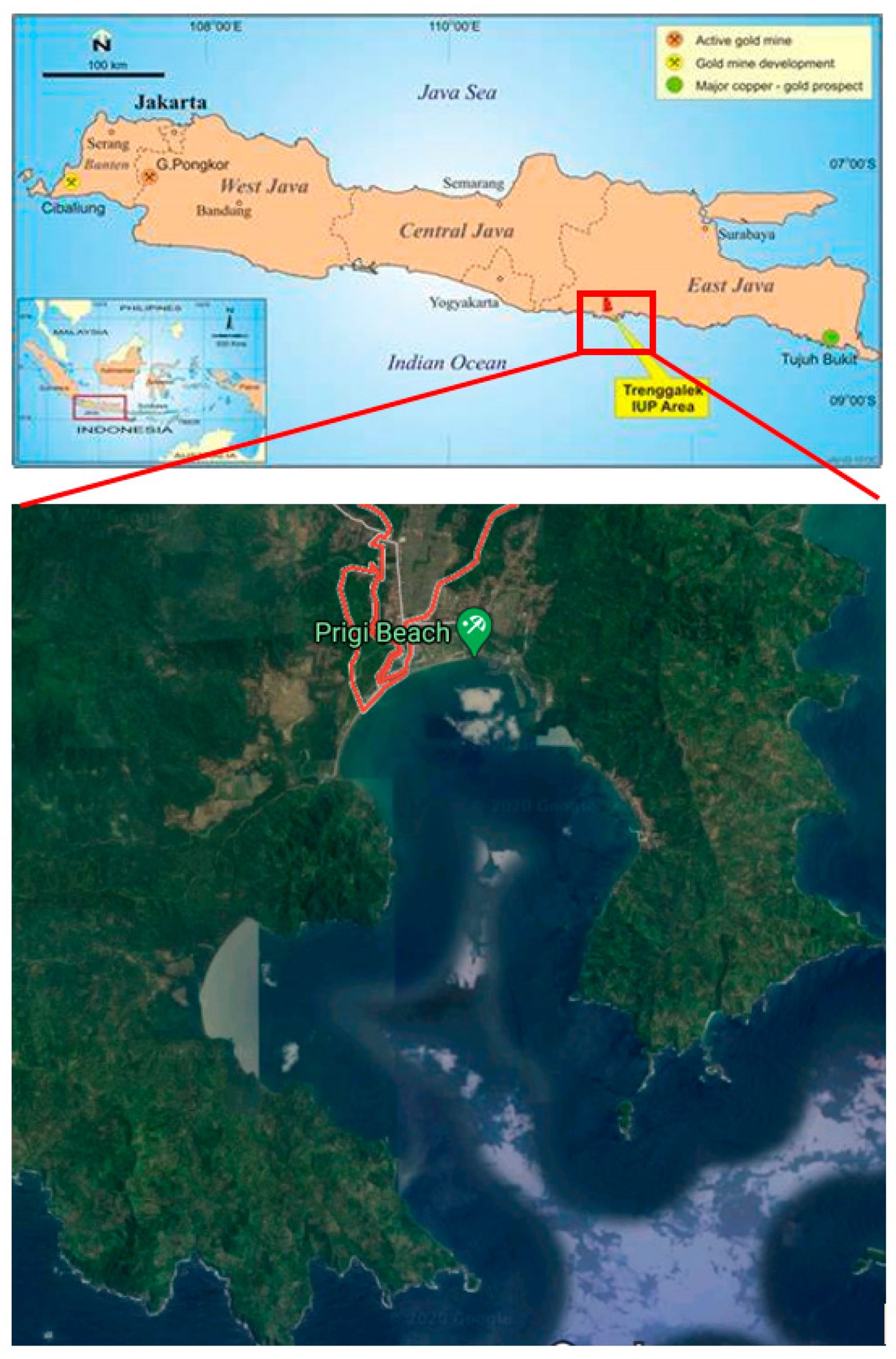
Prigi Bay is situated on the southern coast of the Java Island and is exposed to Indian Ocean. It has a coastline length more than 21 km long. Geographically, Prigi Bay is located at 8°19′39″ S and 111°43′43″ E as shown in Figure 1. The area typically has a tropical climate, with wet and dry seasons. The highest temperature in this area is about 34 °C and lowest temperatures about 25 °C. Generally, Prigi bay is a rocky beach and is surrounded by coral cliffs with height 0–25 m.
3. Materials
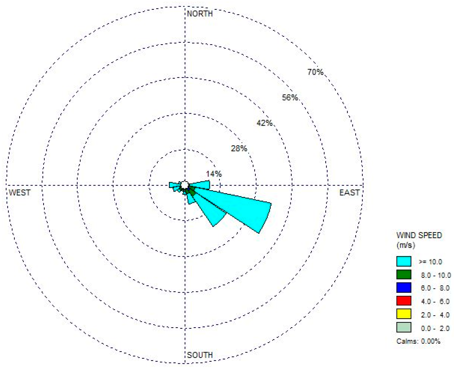
The data in this research is collected from primary and secondary data. Wind data was obtained from the Meteorological, Climatological, and Geophysical Agency (BMKG) during 2004 to 2016. The overall wind speed and direction is shown in Figure 2 below. Figure 2 shows that the dominant wind directions are from the South East (41.92%), East (28.55%) and West (10.48%). In general, the average of wind speed is 10–15 km/h.
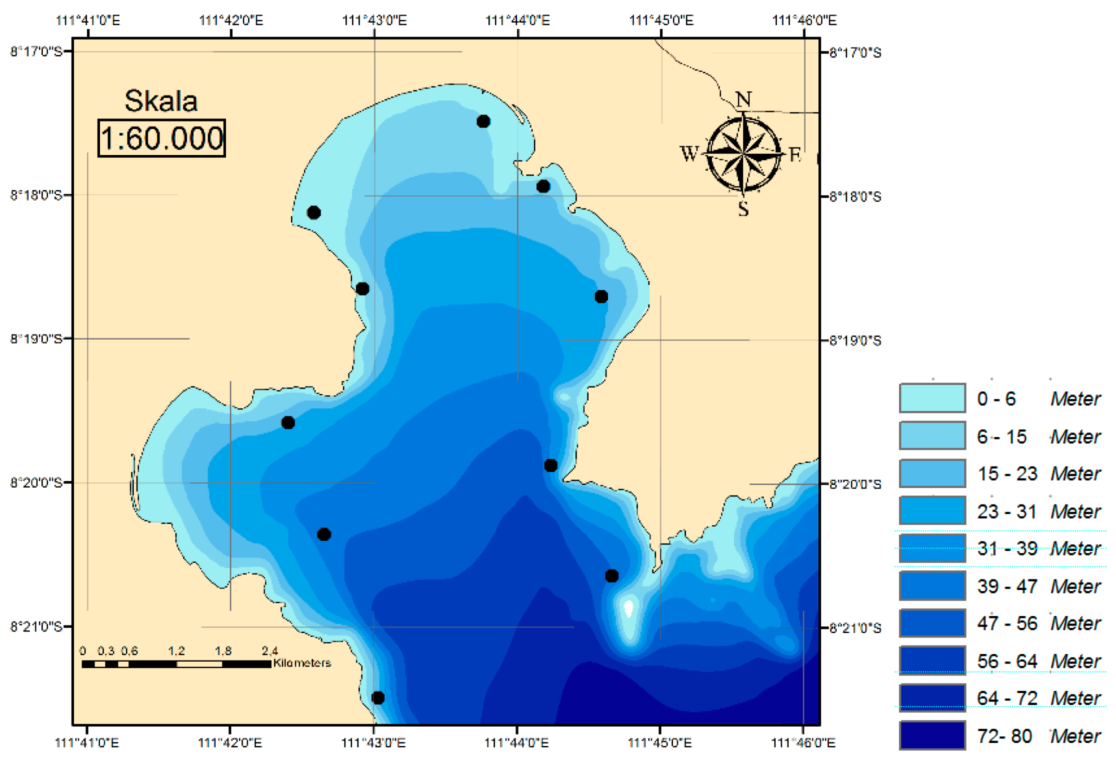
Oceanographic data of bathymetry contour map is obtained from field survey in 2019. The results of the bathymetry map can be seen in the Figure 3.
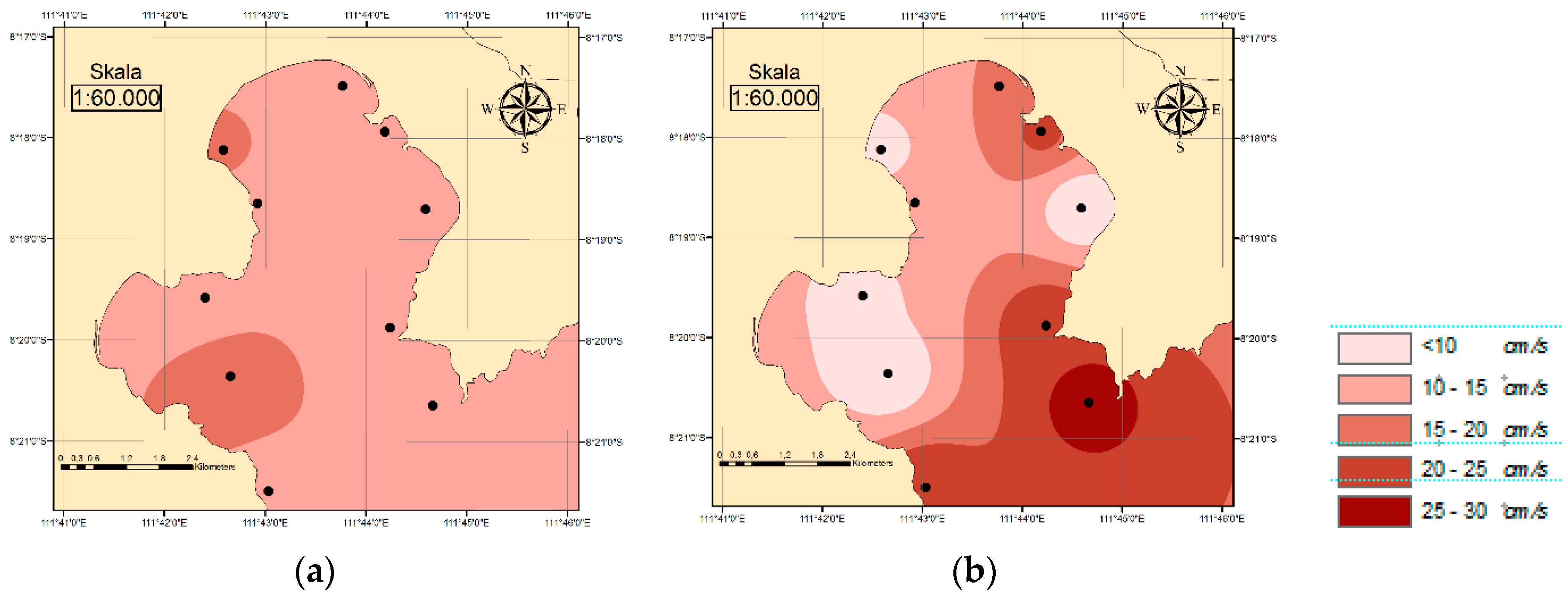
The current velocity on the study location was collected in March and October 2016. Based on the surveyed data [9], it has an uncertain direction and tends to be weak; this is due to the two periods season, including the transitional season. As shown in Figure 4, the current velocity in March had an average speed of 13.38 cm/s, while in October the average speed reached 20.38 cm/s.
4. Methods
4.1. Hydrodynamic Model
The hydrodynamic conditions of the marine area will determine aquaculture sustainability. The components of wave height, current and tidal range are significant information that must be considered before deciding on the location of aquaculture cultivation. Apart from that, the Food and Agriculture Organization (FAO) proposed a site classification for onshore and offshore aquaculture as shown in Table 1. Meanwhile, cage types for specific site class are shown in Table 2.
In this study, environmental parameters used to determine aquaculture location refer to the criteria for cage aquaculture, namely bathymetry, current and wave height as shown in Table 3 below [12,13].
In this study, to obtain the current velocity and sea level elevation, hydrodynamic modeling was completed using Delft3d model. The Delft3D is a hydrodynamic modelling program that is capable of simulating waves, currents, sediment transport, morphological developments and water quality aspects in coastal and ocean areas [14]. Additionally, the Delft3D model can be used in two-dimensions using a depth-averaged (2DH) or three-dimensional (3D) approach [15,16]. In this paper, the model used was 2D using a depth-averaged approach.
The depth-averaged continuity equation is derived by the integration of the continuity equation for incompressible fluids over the total depth, taking into account the kinematic boundary conditions at water surface and bed level [15], and is given by:
where
with U and V the depth averaged velocities
| d | m | depth below some horizontal plane of reference (datum) |
| Gξξ | m | coefficient used to transform curvilinear to rectangular coordinates |
| Gηη | m | coefficient used to transform curvilinear to rectangular coordinates |
| Q | 1/s | global source or sink per unit area |
| qin | 1/s | local source per unit volume |
| qout | 1/s | local sink per unit volume |
| U | m/s | depth-averaged velocity in ξ-direction |
| u | m/s | flow velocity in the y- or ξ-direction |
| V | m/s | depth-averaged velocity in η-direction |
| v | m/s | flow velocity in the x- or η-direction |
| ξ, η | horizontal, curvilinear co-ordinates | |
| ζ | m | water level above some horizontal plane of reference (datum) |
Q representing the contributions per unit area due to the discharge or withdrawal of water, precipitation and evaporation:
with qin and qout the local sources and sinks of water per unit of volume [1/s], respectively, P the non-local source term of precipitation and E non-local sink term due to evaporation.
Model setup and parameters in the DELFT3D-Flow model are summarized in Table 4 below.
4.2. Wave Modeling
4.2.1. Basic Equation
In addition to current velocity and sea level height, the information of wave conditions including the wave height, wave period and wave direction is the most important factor in selecting aquaculture location. The wave parameters in this study were obtained from the wave transformation modelling using the assistance of the CGWAVE model.
CGWAVE transformation wave model is a two-dimensional finite element model based on the wave elliptic-mild slope equation. The CGWAVE model is capable of estimating and simulating wave fields including the effect of breaking waves, refraction, diffraction, reflection in open coastal regions, estuary, around port and islands, and around coastal structures both fixed or floating structures [17]. In this study, the effects of frictional dissipation and wave breaking are neglected. Additionally, this model also does not take into account storm surges event.
The solution of the two-dimensional elliptic mild-slope wave equation can be written as:
where
- (x,y) = complex surface elevation function, from which the wave height can be estimated
- = wave frequency under consideration (in radians/second)
- C(x,y) = phase velocity =
- Cg (x,y) = group velocity =
- with
- k(x,y) = wave number (=2π/L), related to the local depth d(x,y) through the linear dispersion relation:
- = gk tanh (kd)
4.2.2. Setup Boundary Condition
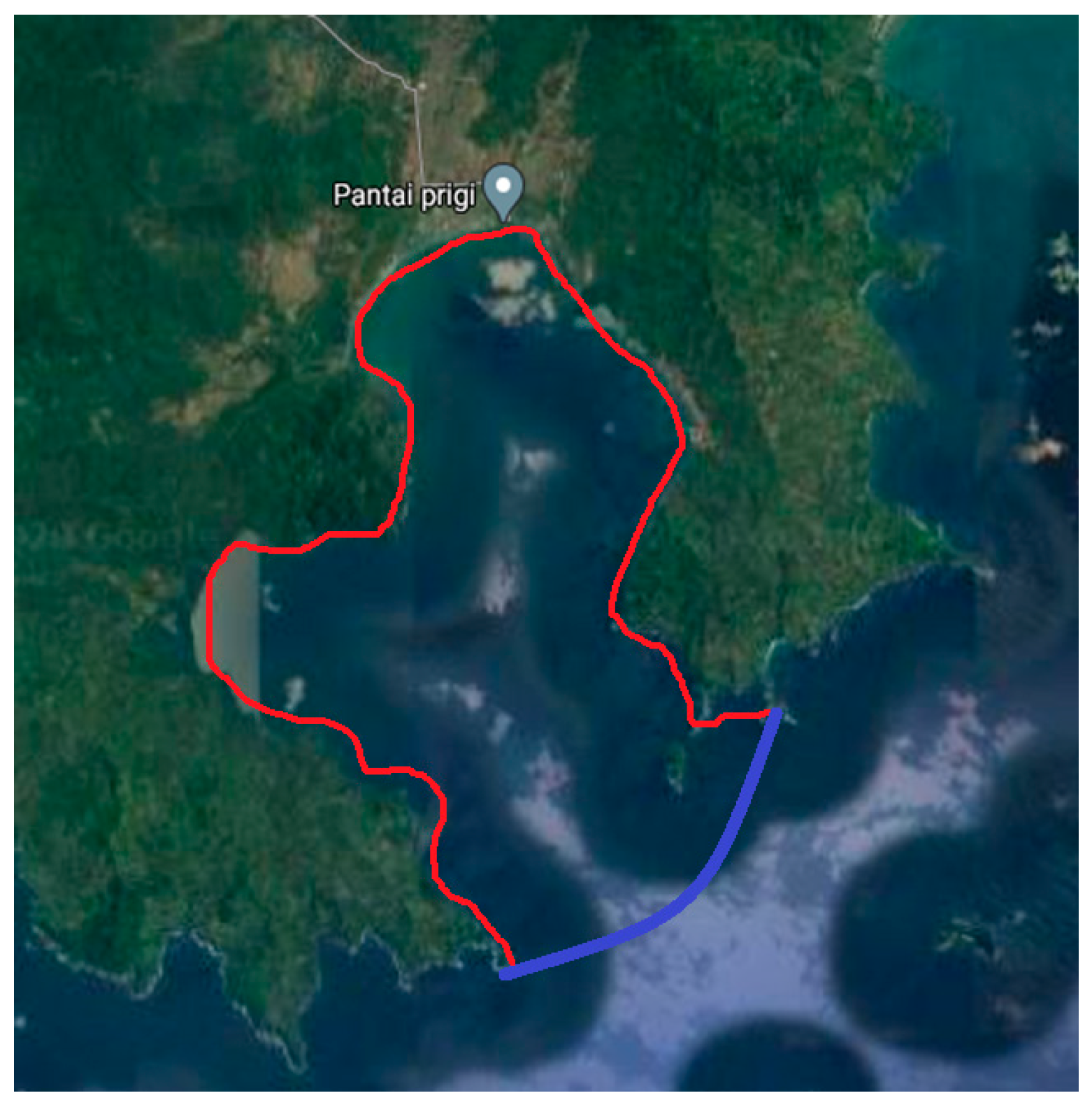
Figure 5 shows the orientation of the CGWAVE model domain of study. The red line represents the model boundaries for the coastline and the blue line is the ocean water boundary. Since the study area is relatively large, the grid size of 5 m was used.
The CGWAVE includes wave reflection from solid boundaries. Reflection coefficients of Cr from 0.0 and 0.5 were selected for the open ocean and land boundary, respectively.
Bathymetric data were collected in August 2019 which indicated depths varying from 2 to 30 m as shown in Figure 3 and were used in CGWAVE. A water level of 1.5 m Mean Lower Low Water (MLLW) was selected as a representative tide in this area.
Twelve different wave conditions were selected for study based on limited field measurements as shown in Table 5. The study used a JONSWAP spectrum with a peak period in the range of 9 to 20 sec. Mean wave directions from South East was used to represent waves propagating.
5. Results and Discussion
5.1. Hydrodynamic Modelling
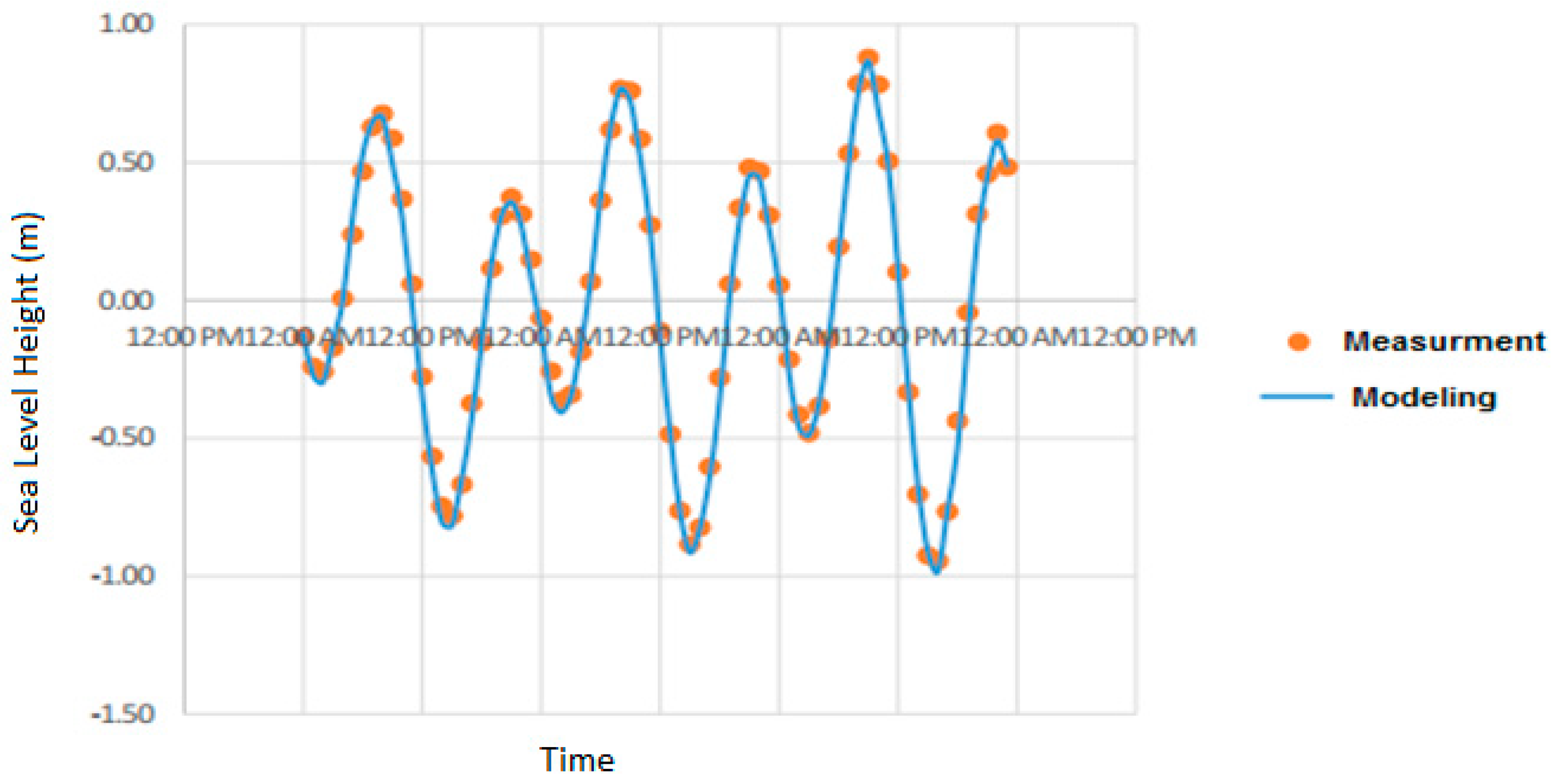
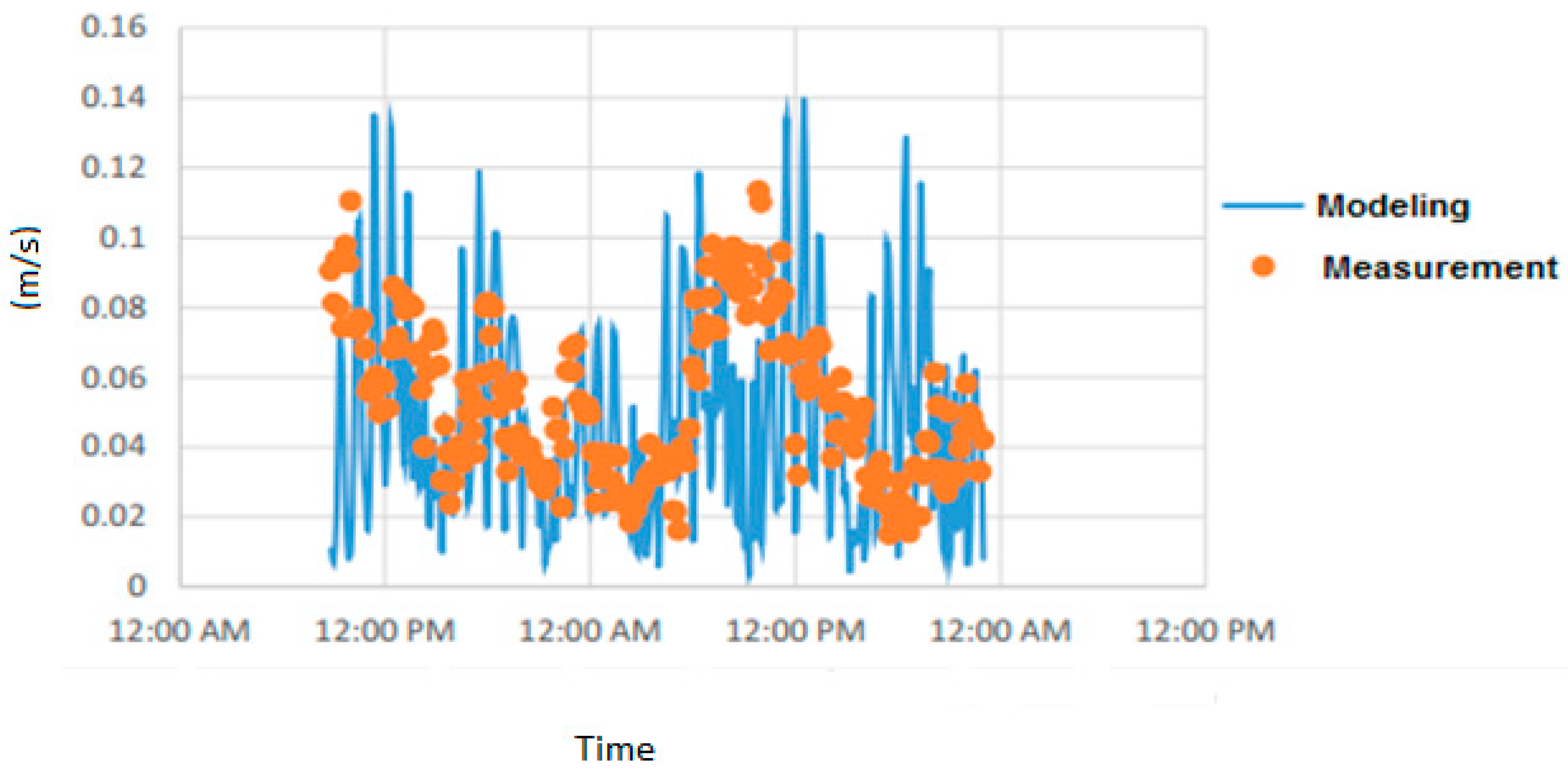
The hydrodynamic model with the Delft3D process-based modeling system simulated water level variations and flows that were generated by astronomical tidal forcing. The model domain is discretized by a structured finite different element. This study used water elevation and current data from measurements to validate the accuracy of model as shown in Figure 6 and Figure 7, respectively.
Figure 6 shows the water level validation between measurement and model. The error between model and measurement is 0.02%. Additionally, the current velocity validation shows an error of 6.70% as shown in Figure 7. Both errors in this model are below 10% which indicates that the model is accurate. The difference that occurs in the current validation between the simulation results and field measurements can be caused by the bathymetry conditions in the model, not yet in accordance with the actual bathymetry conditions because they are the result of interpolation. Apart from that, the influence of wind and the movement of ships around the port can also affect the results of current field measurement.
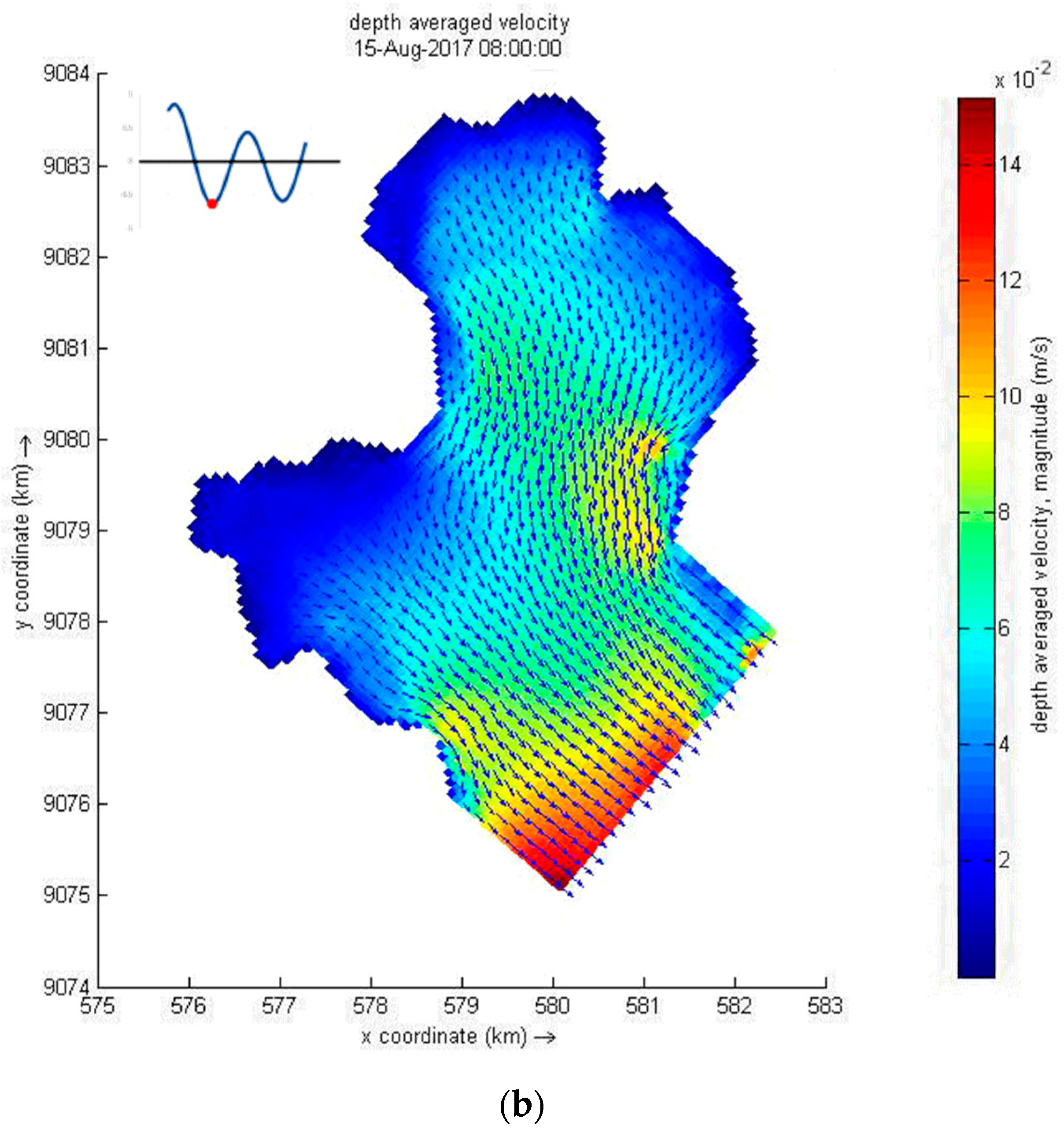
The result of current velocity modelling is presented in Figure 8. The averaged current velocity of flood condition is 0.10 m/s and gradually decreases towards the main body of the Prigi Bay as shown in Figure 8a. Meanwhile, Figure 8b shows the result of current modelling during ebb period. During this period, the averaged current velocity increases towards the open sea with an average value of 0.06 m/s.
5.2. Wave Model
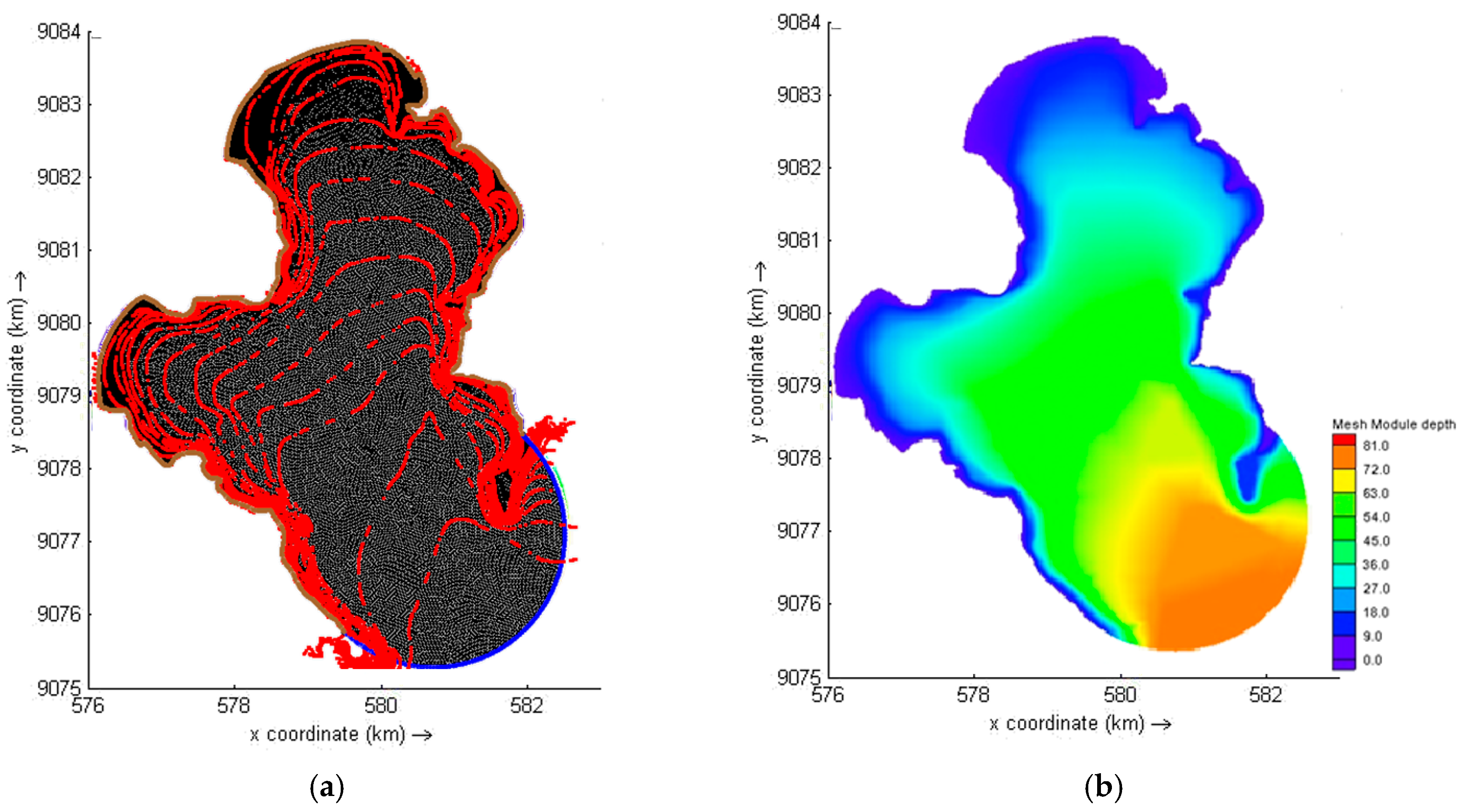
Figure 9a presents a two-dimensional (2D) geometric triangular grid network for finite element calculations using the CGWAVE model where the element sizes must be relevant to the wavelengths to obtain the correct model resolution. The open boundary model used is a semicircular shape for special open boundary treatment and the reflection coefficient that is used on the part of the coastal boundary to the other part of the coast as input data for wave modeling as shown in Figure 5. In this study, CG Wave model is driven by wave height and wave period as shown in Table 5.
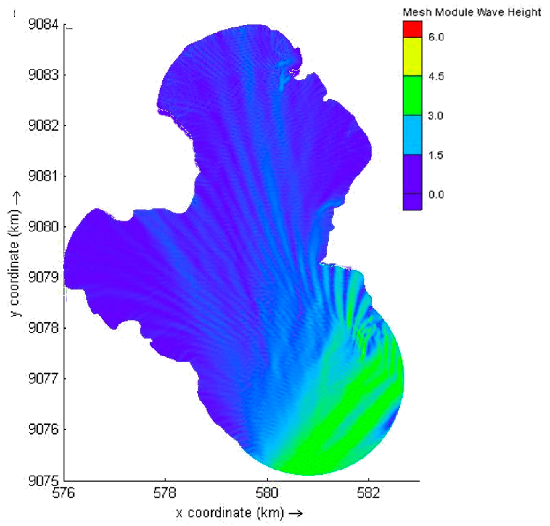
For wave modeling, results in Prigi Bay can be seen in Figure 10. From the results of the wave modeling, the significant wave heights in the Prigi area vary around 0.1–4.5 m with a period of 8.0–8.5 s.
5.3. Suitability Location Using Superimpose Analysis
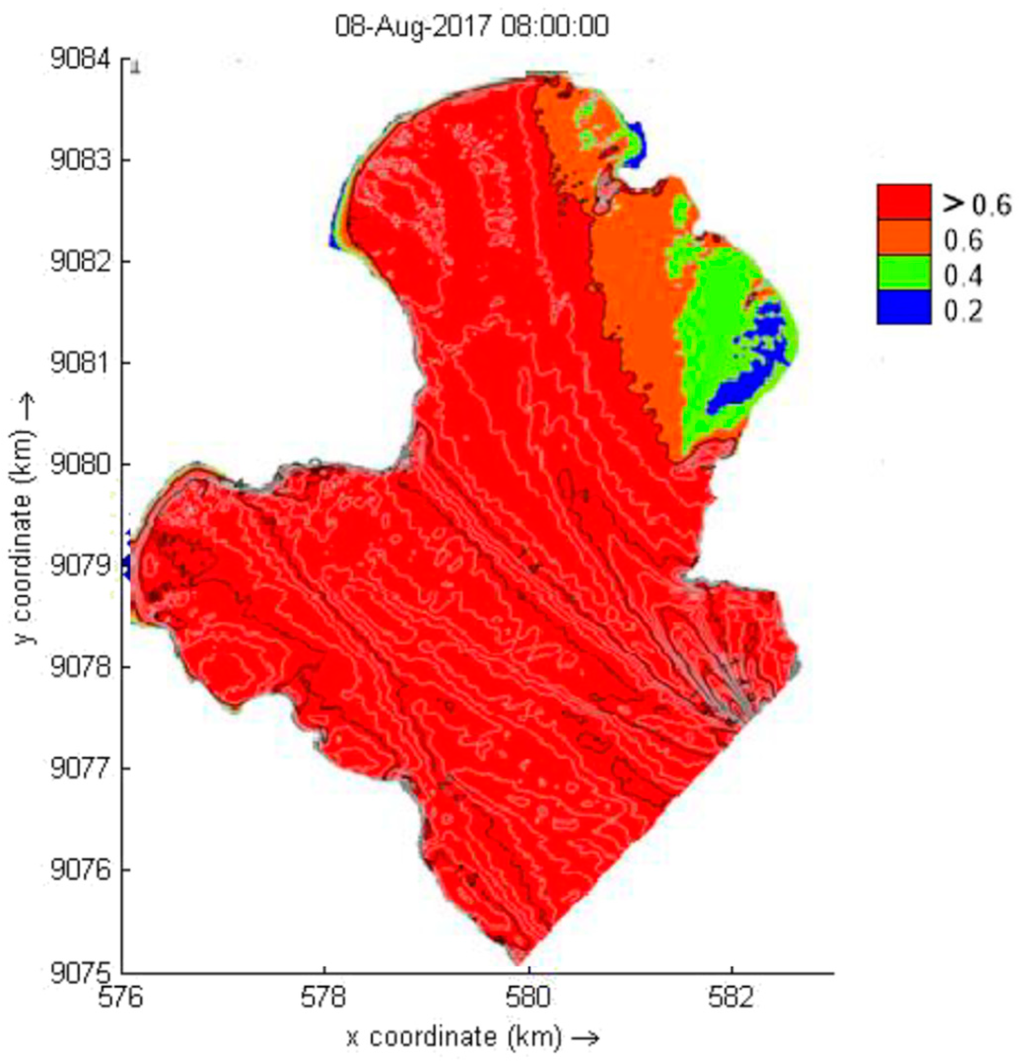
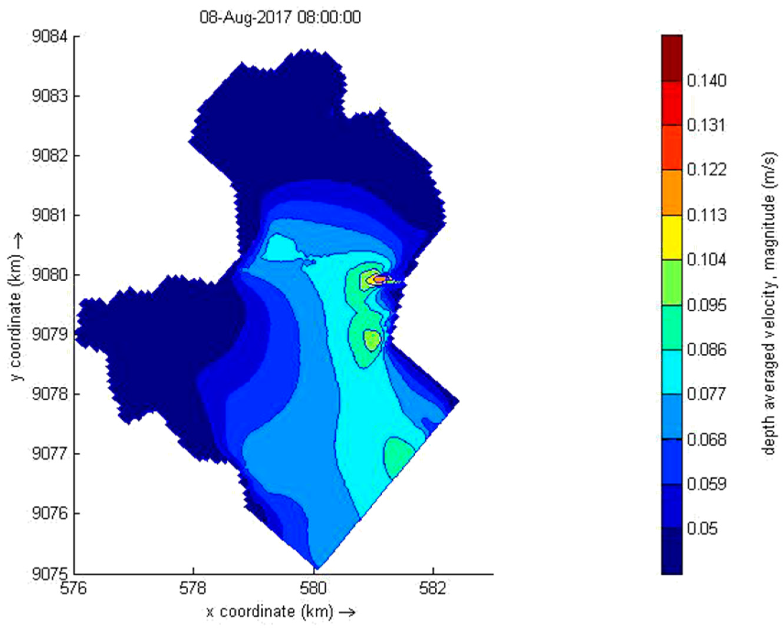
Overlap analysis is used to identify areas that have the potential to develop offshore cultivation based on environmental parameters, especially based on wave and current conditions. Then, the results from each wave height modeling are overlaid with the wave height conditions 0.2–0.4 m. Meanwhile, the results of the current velocity modeling are overlaid to identify a suitable location with the current velocity conditions of 0.05–0.35 m/s. The result of overlap analysis is presented in Figure 11 and Figure 12, respectively.
Figure 11 shows that the locations in green and blue colors are locations where offshore cultivation is feasible, while areas in orange and red indicate that these locations are not suitable for offshore cultivation. The specific location according to the analysis of wave height is in the coastal area with coordinates of 8.301° S–8.317° S and 111.734° E–111.748° E.
Figure 12 shows the results of the overlap analysis of the current velocity. It can be seen that almost all bays are suitable for cultivation sites. Red to light blue color indicates current velocity between 0.05 m/s–0.14 m/s and is a suitable location for cultivation, while the dark blue color is not possible because current velocity is below 0.05 m/s. Low current velocity can inhibit the movement of natural nutrients from the sea which are needed for cultivation.
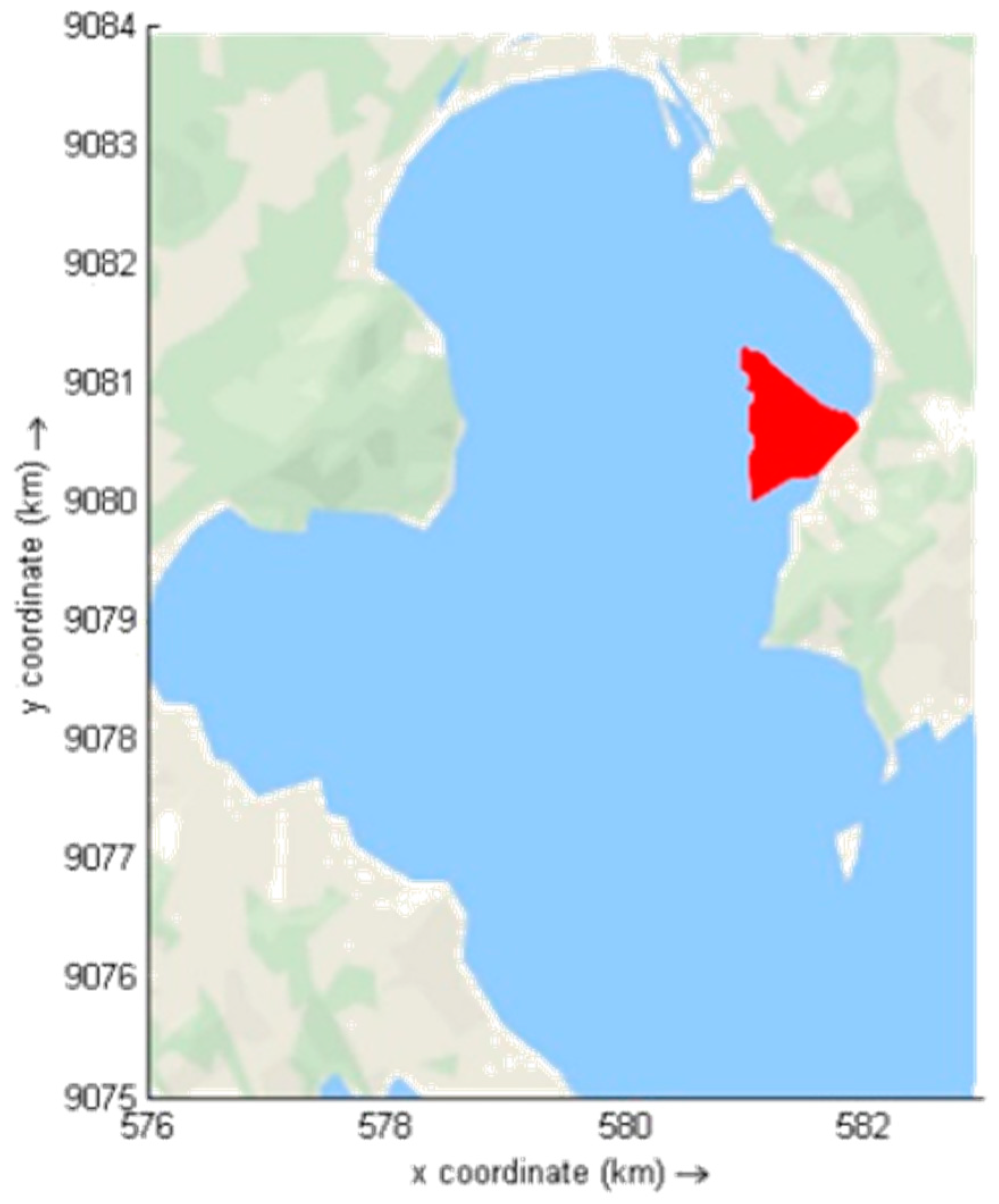
Meanwhile, Figure 13 shows the final analysis of determining the potential location for offshore location based on environmental parameters. Figure 13 shows that the most suitable location for offshore aquaculture is located at coordinate 8.311° S–8.322° S and 111.734° E–111.747° E. This area is protected by a coral cliff from ocean wave force.
6. Conclusions
This study presents numerical wave modeling to investigate the potential area for offshore aquaculture in Prigi Bay. The method used Delft3D Flow and CG WAVE model to simulate wave and current. The superimposed analysis is used to select the potential area between the results of the model and the criteria of environmental parameters. The result showed that the location which meets the aquaculture criteria is located at coordinate 8.311° S–8.322° S and 111.734° E–111.747° E. This site has a depth of around 18–26m with current velocity between 0.1–0.14 m/s and significant wave height between 0.2–0.4m. This location is the most suitable location for aquaculture in the Prigi Bay. In addition, what needs to receive particular attention in supporting offshore cultivation activities in Indonesia is the readiness of infrastructure and logistical support such as main roads, electricity supply, and communication networks. In addition, the legal framework for placing cages for offshore site should also be considered and well prepared.
Author Contributions
Conceptualization, M.Z. and H.D.A.; methodology, M.Z. and H.D.A.; validation, F.P.; writing—original draft preparation, M.Z.; writing—review and editing, M.Z. and H.D.A.; visualization, F.P. All authors have read and agreed to the published version of the manuscript.
Funding
This research was funded by ITS, grant number 925/PKS/ITS/2020.
Conflicts of Interest
The authors declare no conflict of interest.
References
- Ministry of Marine Affairs and Fisheries. Center of Data and Statistics, 2017; Ministry of Marine Affairs and Fisheries: Jakarta, Indonesia, 2018.
- Food and Agriculture Organization of the United States; World Bank. The State of World Fisheries and Aquaculture 2016; Contributing to Food Security and Nutrition for All; Food Agric Organ UN: Rome, Italy, 2016. [Google Scholar]
- Food and Agriculture Organization of the United States; World Bank. Aquaculture Zoning, Site Selection and Area Management under the Ecosystem Approach to Aquaculture A Handbook; Contributing to Food Security and Nutrition for All; Food Agric Organ UN: Rome, Italy, 2017. [Google Scholar]
- Food and Agriculture Organization. The State of World Fisheries and Aquaculture 2020; Sustainability in Action; FAO: Rome, Italy, 2020. [Google Scholar] [CrossRef]
- Duarte, C.M.; Holmer, M.; Olsen, Y.; Soto, D.; Marbà, N.; Guiu, J.; Black, K.; Karakassis, I. Will the oceans help feed humanity? Bioscience 2009, 59, 967–976. [Google Scholar] [CrossRef]
- Zikra, M.; Haryo, D.A.; Billy, M. Site selection of aquaculture location in Indonesia Sea. Ecol. Environ. Conserv. 2020, 26, S8–S17. [Google Scholar]
- Perez, O.M.; Telfer, T.C.; Ross, L.G. Geographical information systems-based models for offshore floating marine fish cage aquaculture site selection in Tenerife, Canary Islands. Aquac. Res. 2005, 36, 946–961. [Google Scholar] [CrossRef]
- Bostick, K. Aquaculture in the Ecosystem. In NGO Approaches to Minimizing the Impacts of Aquaculture: A Review; Holmer, M., Black, K., Duarte, C.M., Marbà, N., Karakassis, I., Eds.; Springer: Dordrecht, The Netherlands, 2008. [Google Scholar]
- Haryo, D.A.; Billy, M.; Zikra, M. The Usage of Geographical Information System in the Selection of Floating Cages Location for Aquaculture at Prigi Bay, Trenggalek Regency, East Java. IOP Conf. Ser. Earth Environ. Sci. 2018, 135, 012023. [Google Scholar]
- Aguilar-Manjarrez, J.; Crespi, V. National Aquaculture Sector Overview Map Collection. User Manual/Vues Générales du Secteur Aquacole National (NASO); Manuel de l’utilisateur; FAO: Rome, Italy, 2013; p. 65. Available online: www.fao.org/docrep/018/i3103b/i3103b00.htm (accessed on 20 November 2020).
- Ryan, J.; Mills, G.; Maguire, D. Farming the Deep Blue; Marine Institute: Dublin, Ireland, 2004; p. 67. [Google Scholar]
- Beveridge, M. Cage Aquaculture, 3rd ed.; Blackwell Publishing: Ames, IA, USA, 2004. [Google Scholar]
- Radiarta, I.N. Mapping the Feasibility of Land Cultivation Sea Fish in District Moro, Riau Islands: With the Geographical Information System Approach. J. Aquac. Res. 2006, 1, 291–302. [Google Scholar]
- Roelvink, J.A.; Van Banning, G.K.F.M. Design and development of Delft3D and application to coastal morphodynamics. In Proceedings of the Hydroinformatics ’94 Conference, Delft, The Netherlands, 19–23 September 1994. [Google Scholar]
- Deltares. Delft3D-FLOW Manual; Boussinesqweg: Delft, The Netherlands, 2014. [Google Scholar]
- Elias, E.P.L.; Walstra, D.-J.; Dano, J.A. Roelvink and Marcel Stive, Hydrodynamic Validation of Delft3D with Field Measurements at Egmond. In Proceedings of the 27th International Conference on Coastal Engineering (ICCE), Sydney, Australia, 16–21 June 2001. [Google Scholar]
- Demirbilek, Z.; dan Panchang, V. CGWAVE: A Coastal Surface Water Wave Model of the Mild Slope Equation; Army Corps of Engineers: Washington, DC, USA, 1998.
Figure 1.
The location of Prigi Bay in east Java Province.

Figure 2.
Windrose in Prigi Bay.

Figure 3.
Bathymetry in Prigi Bay.

Figure 4.
Distribution of Current Velocity (a) March (b) October 2016.

Figure 5.
Boundary condition for Prigi Bay (red line is land boundary and blue line is open ocean boundary).
Figure 5.
Boundary condition for Prigi Bay (red line is land boundary and blue line is open ocean boundary).

Figure 6.
Delft3D modelled and measured water level.

Figure 7.
Delft3D modelled and measured current velocity.

Figure 8.
Current velocity model results (a) flood tide (b) ebb tide.


Figure 9.
Finite Element Meshing (a) and Bathymetry Prigi Bay (b).

Figure 10.
Results Wave Height Modeling in January.

Figure 11.
Results Overlay Modeling of Wave 12 Months.

Figure 12.
Current Modeling Overlay Results.

Figure 13.
Suitable Area for Offshore Aquaculture (red area).


Table 1.
Site classification proposed by the Food and Agriculture Organization (FAO) in 2009 (source: [10]).
Table 1.
Site classification proposed by the Food and Agriculture Organization (FAO) in 2009 (source: [10]).
| Parameter | Coastal | Off the Coast | Offshore |
|---|---|---|---|
| Location | 500 m from the coast | 500 m–3 km | >3 km open ocean |
| Depth | 10 m depth | 10 m < depth < 50 m | 50 m depth< |
| Wave Height | Hs < 1 m | Hs < 3–4 m | Hs > 5 m |
Table 2.
Marine cage site classification [11].
Table 2.
Marine cage site classification [11].
| Site Class | 1 | 2 | 3 | 4 |
|---|---|---|---|---|
| Conventional description | Sheltered inshore site | Semi-exposed inshore site | Exposed offshore site | Open-ocean offshore site |
| Cage type used | Surface gravity | Surface gravity | Surface gravity, anchor tension | Surface gravity, surface rigid, anchor tension, submerged gravity, submerged rigid |
Table 3.
Environmental parameters for aquaculture.
| Environmental Parameter | Unit | Highly Suitable | Suitable | Unsuitable |
|---|---|---|---|---|
| Bathymetry | m | 10–20 | 20–30 | <10 >30 |
| Current | m/s | 0.05–0.15 | 0.15–0.35 | >0.35 <0.05 |
| Wave Height | m | <0.20 | 0.20–0.40 | >0.40 |
Table 4.
Model Setup and Parameters.
| No | Parameters | |
|---|---|---|
| 1 | Delft3D model setup | |
| Model configuration | 2DH (depth-averaged) | |
| Horizontal grid resolution | 20 m × 20 m | |
| Number of grid elements | 9760 | |
| Meteorological forcing | astronomical tidal forcing, wind data | |
| 2 | Delft3D parameters | |
| Time step | 60 s | |
| Chézy roughness coefficient | 65 m1/2/s | |
| Horizontal eddy viscosity | 1 m2/s | |
| Horizontal eddy diffusivity | 1 m2/s | |
| Threshold depth | 0.1 m |
Table 5.
Wave Height and Wave Period.
| Month | Wave Height (m) | Wave Period (s) |
|---|---|---|
| January | 3.68 | 9.95 |
| February | 3.89 | 10.82 |
| March | 3.54 | 17.68 |
| April | 2.73 | 15.53 |
| May | 3.17 | 16.91 |
| June | 3.54 | 17.68 |
| July | 3.86 | 20.13 |
| August | 3.59 | 18.85 |
| September | 2.88 | 15.62 |
| October | 2.52 | 15.62 |
| November | 2.22 | 11.28 |
| December | 2.40 | 12.23 |
Publisher’s Note: MDPI stays neutral with regard to jurisdictional claims in published maps and institutional affiliations. |
© 2020 by the authors. Licensee MDPI, Basel, Switzerland. This article is an open access article distributed under the terms and conditions of the Creative Commons Attribution (CC BY) license (http://creativecommons.org/licenses/by/4.0/).
Share and Cite
MDPI and ACS Style
Zikra, M.; Armono, H.D.; Pratama, F. Wave Modeling for the Establishment Potential Area of Offshore Aquaculture in Indonesia. Fluids 2020, 5, 229. https://doi.org/10.3390/fluids5040229
AMA Style
Zikra M, Armono HD, Pratama F. Wave Modeling for the Establishment Potential Area of Offshore Aquaculture in Indonesia. Fluids. 2020; 5(4):229. https://doi.org/10.3390/fluids5040229
Chicago/Turabian StyleZikra, Muhammad, Haryo Dwito Armono, and Fahrizal Pratama. 2020. "Wave Modeling for the Establishment Potential Area of Offshore Aquaculture in Indonesia" Fluids 5, no. 4: 229. https://doi.org/10.3390/fluids5040229