Geomechanical Response of Fractured Reservoirs
by
 ,
,
Ahmad Zareidarmiyan
1,2,3,* ,
,
Hossein Salarirad
1,*,
Victor Vilarrasa
2,3,
Silvia De Simone
2,3,4 and
Sebastia Olivella
5 1
Department of Mining and Metallurgical Engineering, Amirkabir University of Technology—Tehran Polytechnic (AUT), Tehran 15875-4413, Iran
2
Institute of Environmental Assessment and Water Research (IDAEA), Spanish National Research Council (CSIC), 08034 Barcelona, Spain
3
Associated Unit: Hydrogeology Group UPC-CSIC, 08034 Barcelona, Spain
4
Department of Earth Science & Engineering, Imperial College London, London SW7 2AZ, UK
5
Department of Civil and Environmental Engineering, Technical University of Catalonia (UPC-BarcelonaTech), 08034 Barcelona, Spain
*
Authors to whom correspondence should be addressed.
Fluids 2018, 3(4), 70; https://doi.org/10.3390/fluids3040070
Submission received: 15 August 2018
/
Revised: 24 September 2018
/
Accepted: 27 September 2018
/
Published: 29 September 2018
(This article belongs to the Special Issue Fundamentals of CO2 Storage in Geological Formations)
Abstract
:Geologic carbon storage will most likely be feasible only if carbon dioxide (CO2) is utilized for improved oil recovery (IOR). The majority of carbonate reservoirs that bear hydrocarbons are fractured. Thus, the geomechanical response of the reservoir and caprock to IOR operations is controlled by pre-existing fractures. However, given the complexity of including fractures in numerical models, they are usually neglected and incorporated into an equivalent porous media. In this paper, we perform fully coupled thermo-hydro-mechanical numerical simulations of fluid injection and production into a naturally fractured carbonate reservoir. Simulation results show that fluid pressure propagates through the fractures much faster than the reservoir matrix as a result of their permeability contrast. Nevertheless, pressure diffusion propagates through the matrix blocks within days, reaching equilibrium with the fluid pressure in the fractures. In contrast, the cooling front remains within the fractures because it advances much faster by advection through the fractures than by conduction towards the matrix blocks. Moreover, the total stresses change proportionally to pressure changes and inversely proportional to temperature changes, with the maximum change occurring in the longitudinal direction of the fracture and the minimum in the direction normal to it. We find that shear failure is more likely to occur in the fractures and reservoir matrix that undergo cooling than in the region that is only affected by pressure changes. We also find that stability changes in the caprock are small and its integrity is maintained. We conclude that explicitly including fractures into numerical models permits identifying fracture instability that may be otherwise neglected.
1. Introduction
The implementation of geologic carbon storage may be hindered by its cost. For this reason, it has been proposed that the injected carbon dioxide (CO2) should be utilized to make it feasible, leading to Carbon Capture, Utilization and Storage (CCUS). Enhanced Oil Recovery (EOR) methods as a part of Improved Oil Recovery (IOR) [1] is a utilization option that is already been used, like at Weyburn, Canada. Large amounts of hydrocarbons remain worldwide in reservoirs in which conventional recovery methods become ineffective and IOR techniques are necessary. Much of the remaining hydrocarbons are found in naturally fractured reservoirs (NFRs). The expected recovery depends on the chosen method, which is selected based on criteria such as technical limits and economic shortage [2,3]. IOR methods imply the injection of fluids that induce pressure and temperature changes in the reservoir. These changes cause a geomechanical response of the subsurface that may compromise reservoir stability and caprock integrity [4,5,6].
Fluid injection results in pore pressure increase and temperature drop that reduces the effective stresses, bringing the stress state closer to failure conditions. On the one hand, if tensile failure is reached, hydraulic fractures will be created. On the other hand, if shear failure occurs, pre-existing fractures will slip, opening up due to dilation. Thus, both failure modes will cause permeability increase. Such permeability increase enhances the efficiency of IOR operations if it occurs within the reservoir, but it may be problematic if it extends into the caprock.
To accurately assess the geomechanical response of the subsurface to IOR operations, the characteristics of the reservoir should be taken into account. A large portion of conventional oil and gas reserves are found in carbonate rocks, which are higly fractured [7]. Nevertheless, NFRs are usually considered as an equivalent continuous porous media. Thus, the impact of fractures on fluid flow and geomechanics is usually neglected. However, this simplification may be a non-reasonable assumption in some cases, like in carbonate oil reservoirs [8,9].
Coupled thermal-hydro-mechanical (THM) processes in geological fractured media entail complex interactions between the processes [4,10,11,12,13,14,15]. Modeling these coupled THM processes in fractured media requires numerical simulators that solve the three processes in a fully coupled way or a fluid flow code coupled to a geomechanical code. Several codes capable of simulating NFRs have been developed in the last decades, such as OpenGeoSys [16], ABAQUS [17], FLAC [18], UDEC and 3DEC [19], CODE_BRIGHT [20,21], and RDCA-TOUGH2 [22,23].
The aim of this study is to investigate the effects of IOR methods, as a potential option for CCUS, on deep fractured geological media. To this end, we model a NFR, including two sets of prependicular fractures, and simulate production of the reservoir fluid and fluid injection at a colder temperature than that of the rock. By representing single fractures using an embedded model available in CODE_BRIGHT, we study THM coupled processes induced by low-temperature injection during IOR operations in a deep naturally fractured carbonate reservoir. First, we introduce the coupled THM mathematical formulation of non-isothermal multiphase flow in deformable fractured media. Next, we simulate injection of low-temperature fluid into a fractured reservoir for a range of fracture permeability. Finally, we draw conclusions on how temperature and fluid pressure changes affect effective stresses and thus, fracture stability and caprock integrity.
2. Methods
2.1. Geometry
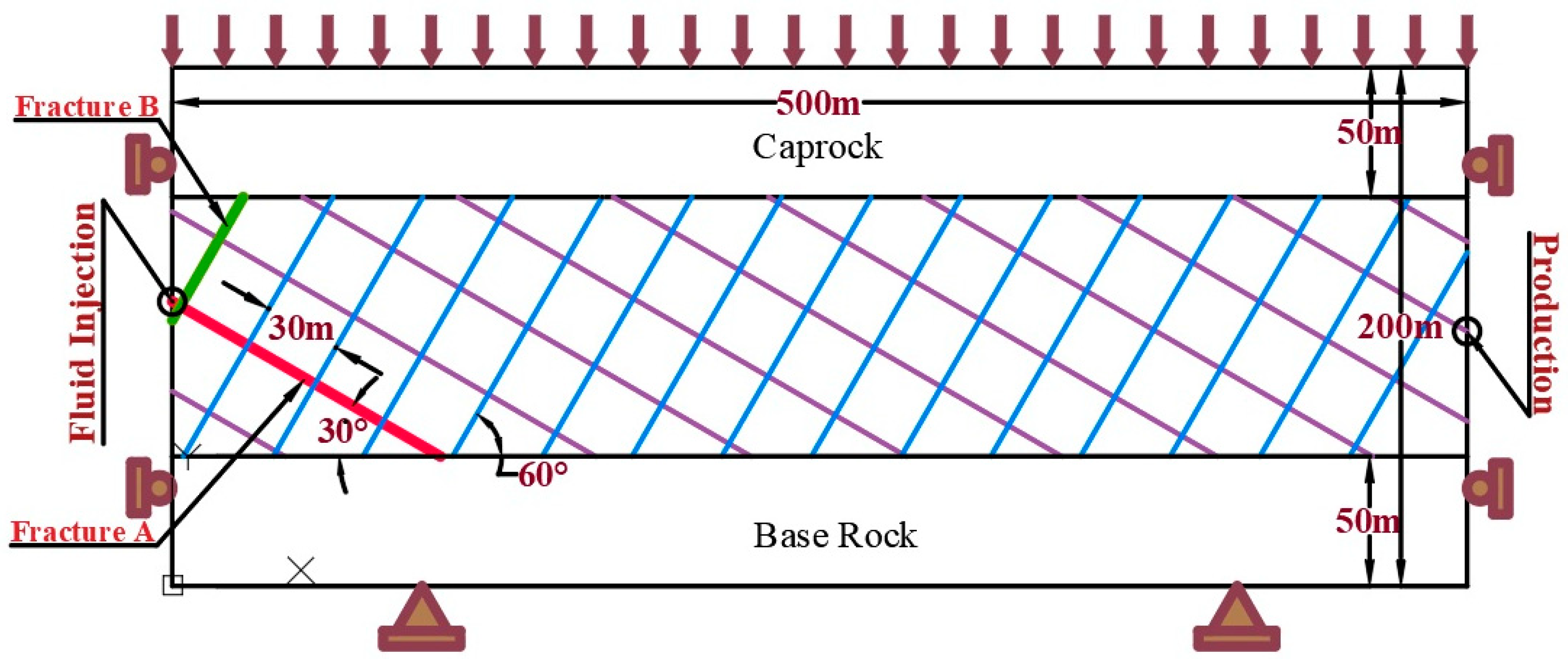
We model an IOR operation into a NFR by using an idealized cross-section with plane strain conditions. The model consists of three horizontal layers that represent the caprock, reservoir, and bedrock with thickness of 50, 100, and 50 m, respectively. The reservoir, which corresponds to a carbonate reservoir, includes two sets of planar fractures that are perpendicular between them and have and dip angles and 30 m spacing (Figure 1). Injection into the reservoir takes place through a horizontal well on one side of the model and production takes place on the other side of the model. These two wells intersect fractures. We simulate both water and CO2 injection. The top of the caprock is located at a depth of 3000 m. The height and length of the model are 200 and 500 m, respectively.
2.2. Modeling Discontinuities
Fractures are modeled as single fractures embedded in a continuous porous medium and are characterized by their aperture, which defines the fracture permeability by means of the traditional cubic law. In this study, we consider that fracture permeability remains constant throughout the whole simulation period. Fluid flow through a single fracture can be expressed by Darcy’s law [24,25,26]
where is the volumetric flux of α-phase (volume of fluid per unit area per unit time), is the intrinsic permeability, is the relative permeability of α-phase, and are dynamic viscosity and density of α-phase, respectively, which are functions of pressure and temperature, is temperature, is the pressure of α-phase, is the gravity, is the elevation and α is either water, w, or CO2, c.
The flow rate per unit width of a fracture can be calculated from Darcy’s law, which assuming that the permeability of fractures is controlled by fracture aperture, b [L], becomes the cubic law [27]
To assess fracture stability, we adopt the Drucker-Prager yield criteria. In terms of effective stress tensor and deviatoric stress, the yield function reads
where is the deviatoric stress, is the mean effective stress and is cohesion. Parameters and depend on the stress. Assuming a normal faulting stress regime in which the vertical stress is the maximum, they are given by
where is the internal friction angle. While denotes elastic behavior, implies both elastic and plastic strain.
2.3. THM Mathematical and Numerical Model
Simulation of non-isothermal two phase flow requires the simultaneous solution of mass conservation for each phase, energy balance, and momentum balance. Assuming no chemical reactions, fluid conservation can be expressed as [25]
where is time, φ [L3L−3], is saturation of α-phase, and is the source/sink term of α-phase. Momentum conservation of the fluid phase in a porous media is expressed using Darcy’s law (Equation (1)).
Non-isothermal effects are governed by energy balance, which is given by reference [28]
where is solid density, is enthalpy of the solid, is enthalpy of α-phase and is thermal conductivity of the geological medium. Thermal equilibrium of all phases is assumed at every point.
To solve the mechanical problem, the equilibrium equation for a porous medium has to be satisfied. Assuming quasi-static conditions, i.e., neglecting inertial terms, momentum balance results in equilibrium of stresses
where is the stress tensor and is the body forces vector.
We assume that the medium behaves elastically and adopt linear poro-thermoelasticity, using the sign criterion of geomechanics, i.e., strain is positive in compression and negative in extension, to acknowledge the effect of changes in fluid pressure and temperature on the geomechanical response [29,30]
where is the strain tensor, is the Young’s modulus, is Poisson ratio, is the mean stress, is the total stress in the direction , is the identity matrix, is the maximum fluid pressure, i.e., , and is the linear thermal expansion coefficient. The volumetric strain is defined as
where is the mean effective stress and is the bulk modulus.
Subsequently, the effective stress tensor can be expressed as a function of changes in strain, pressure, and temperature as [29,31]
where is the shear modulus. Note that we have also assumed a Biot’s coefficient equal to 1, which means that the compressibility of the rock is negligible compared to that of the drained bulk material
2.4. Model Setup
The parameters used for the simulations are shown in Table 1. Initial conditions correspond to hydrostatic pressure, a geothermal gradient of with a surface temperature of and a stress state that corresponds to a normal faulting regime; i.e., the vertical stress is greater than the horizontal stresses, following the relationship .
The mechanical boundary conditions are the lithostatic stress on the upper boundary, no displacement perpendicular to the lateral boundaries and fix displacement in the lower boundary. Initial and boundary conditions and a schematic representation of the geometry are shown in Figure 1. Water or CO2 are injected in the reservoir through a fracture with a prescribed constant pressure increase of for 365 days. We use single phase simulations injecting water with the aim to understand the geochemical response of NFRs to fluid injection and production. Then, we compare the results to those of CO2 injection to investigate the implications for CO2 storage. For CO2 injection, we only consider fracture permeability equal to 10−14 m2. The injected fluid is at a temperature of , which means that it is some colder than the reservoir. The production well is placed on the opposite lateral boundary and has a prescribed pressure decrease of on a fracture within the reservoir.
The mesh is made of unstructured quadrilateral elements and is refined in the areas where fractures intersect. The fractures are modeled with 0.1 m-thick features. The size of the elements in the fracture is 0.1 m and it progressively increases further away, reaching a size of 4 m in the reservoir, caprock, and base rock. As a first step, a steady-state calculation is carried out to achieve consistent initial conditions in equilibrium for the pressure, temperature, and stress fields. Simulations are performed with CODE_BRIGHT [20,21], which is a finite element numerical code that solves fully coupled THM problems in porous media.
3. Results
3.1. Fluid Pressure Evolution
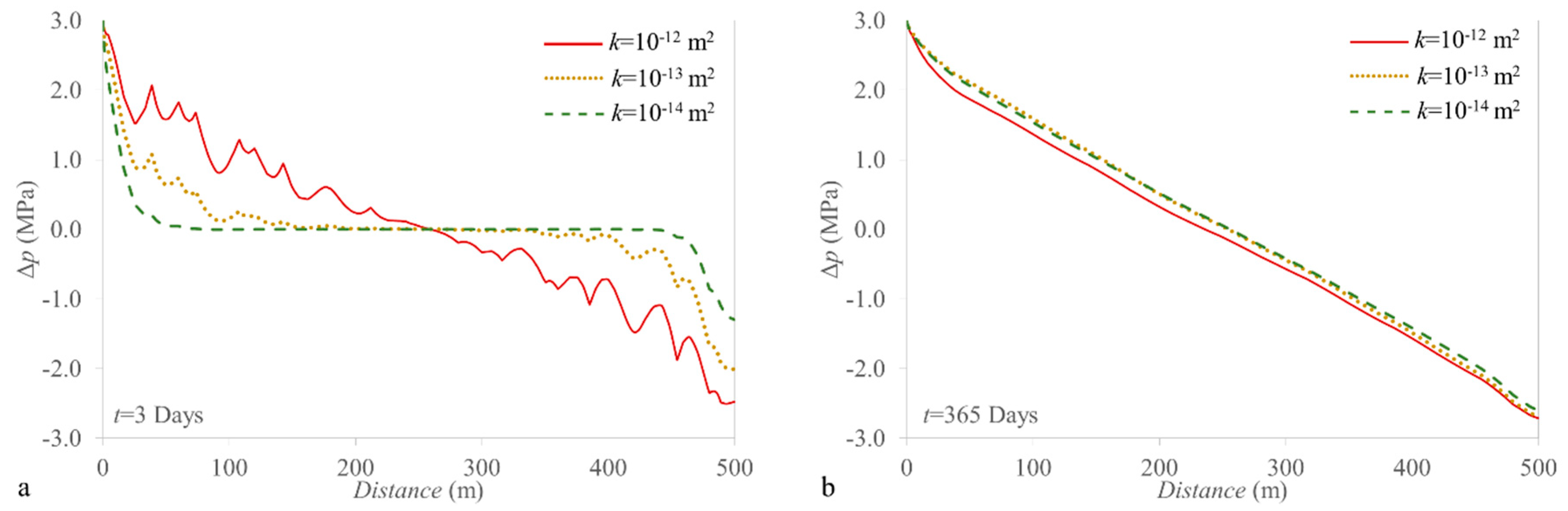
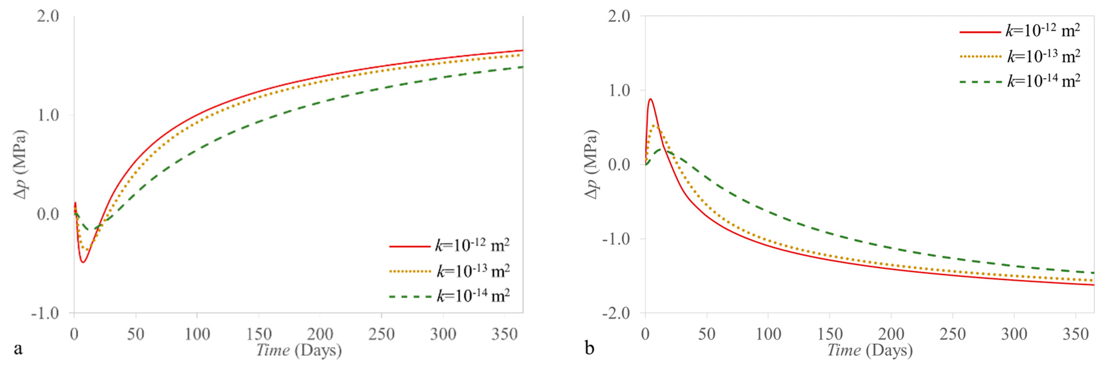
Changes in fluid pressure as a result of injection/production extend further in the fractures than in the reservoir matrix due to the large permeability contrast between them. During the first days of operation, pressure changes mainly occur in the fractures (Figure 2 and Figure 3). The pressure fluctuations are observed (Figure 3a) because of the diffusion time differences between the fractures and the reservoir matrix. Actually, fracture permeability plays a dominant role in pressure diffusion along the reservoir. The higher the fracture permeability, the faster the pressure propagates through the fractures. After three days of operation, the pressure front propagates through the whole reservoir when the fracture permeability is of 10−12 m2, whereas it only propagates for a quarter of the reservoir length for the case with fracture permeability of 10−13 m2, and even less when permeability is 10−14 m2. When the fluid flow reaches steady state (Figure 3b), the pressure change profiles are the same regardless of the fractures intrinsic permeability. The small differences between the intrinsic permeability of 10−12 m2 and the less permeable cases are due to the fact that cooling propagates further for more permeable fractures, which leads to a steeper pressure gradient because of the higher viscosity of colder water (see Section 3.2).
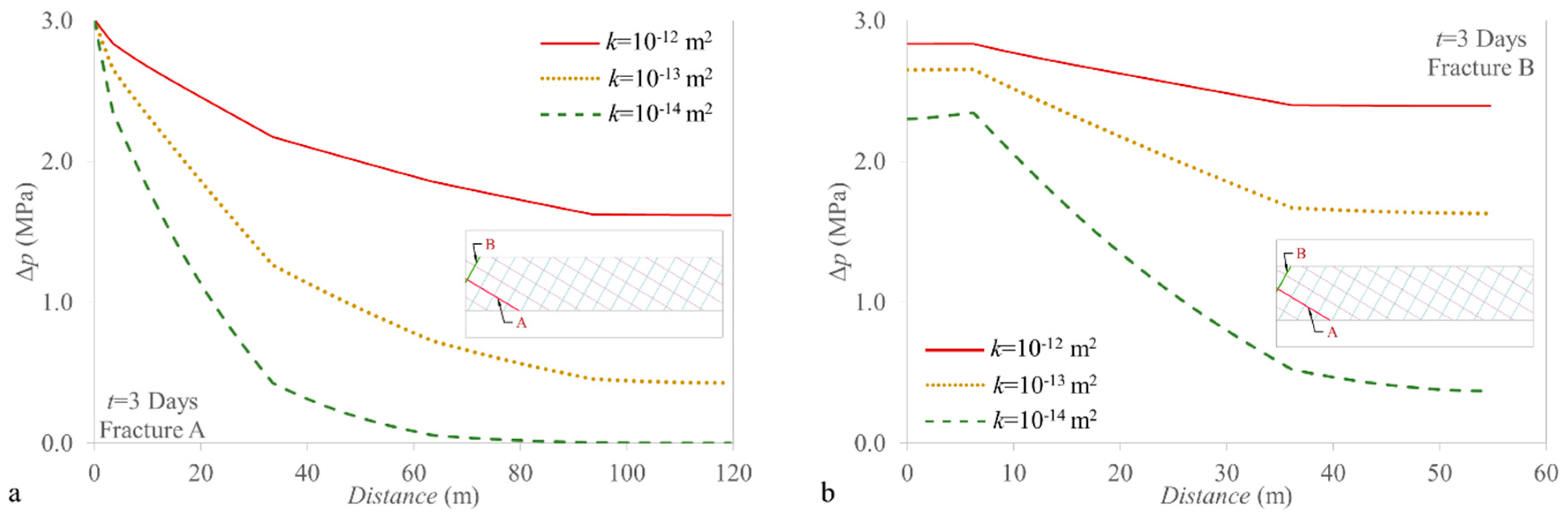
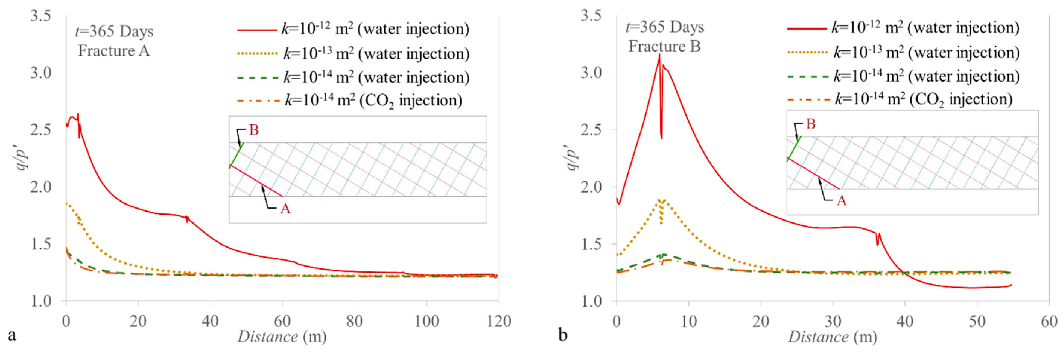
Figure 2 compares the fluid pressure changes as a function of the distance in two fractures close to the injection point with dip angles of −30° and 60° degrees (fractures A and B in Figure 1) after 3 days of operation for three intrinsic permeability of fractures. The reason for the different pressure profiles in fractures A and B is that fluid is injected in A, and not in B, so the first portion of fracture B receives fluid (the gradient points towards the left), instead of giving fluid as in fracture A, where injection takes place.
Given the constant prescribed injection pressure and the fixed intrinsic permeability of the reservoir matrix, the flow rate increases for higher permeability of the fractures. As a result, temperature and pore pressure propagate further for higher contrast between the intrinsic permeability of the fractures and the matrix blocks. Once the steady-state in the pressure profile is reached, cooling advances faster for higher fracture permeability.
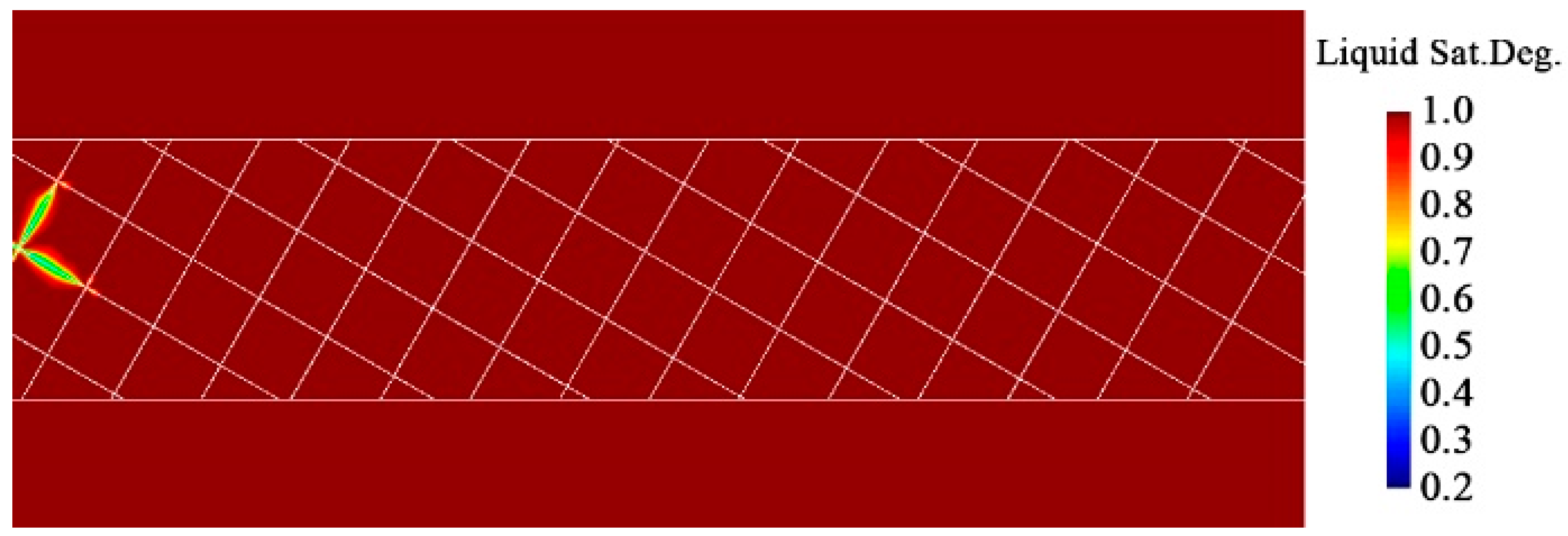
If CO2 is injected, the pressure evolution is similar to that of water injection. CO2 mainly advances through the fractures because the penetration into the matrix blocks is hindered by their entry pressure (Figure 4). Even though some CO2 gets into the matrix blocks, the CO2 saturation degree is small. The CO2 advance through the fracture network is limited by the low permeability of the fractures. A higher fracture permeability and a longer injection time would lead to a larger presence of CO2 in the fracture network and into the matrix blocks. Yet, the CO2 storage capacity seems to be limited in fractured reservoirs unless the entry pressure of the matrix blocks is very low.
Figure 5 depicts the evolution of fluid pressure at the bottom of the caprock during one-year of operation above the injection and production wells. Fluid pressure changes inversely proportional to the volumetric strain change in the caprock. When injection starts, the pore volume increases above the injection well and decreases above the production well in the lower part of the caprock as a result of caprock bending. After several days of injection, the pore pressure reverses its tendency because of pressure diffusion into the caprock. This phenomenon, which is known as the “Noordbergum effect”, leads to a reverse-fluid level fluctuation that is well known and documented in confined aquifers [32,33,34]. This effect can only be captured if hydro-mechanical (HM) or THM processes are taken into account.
3.2. Non-Isothermal Effects
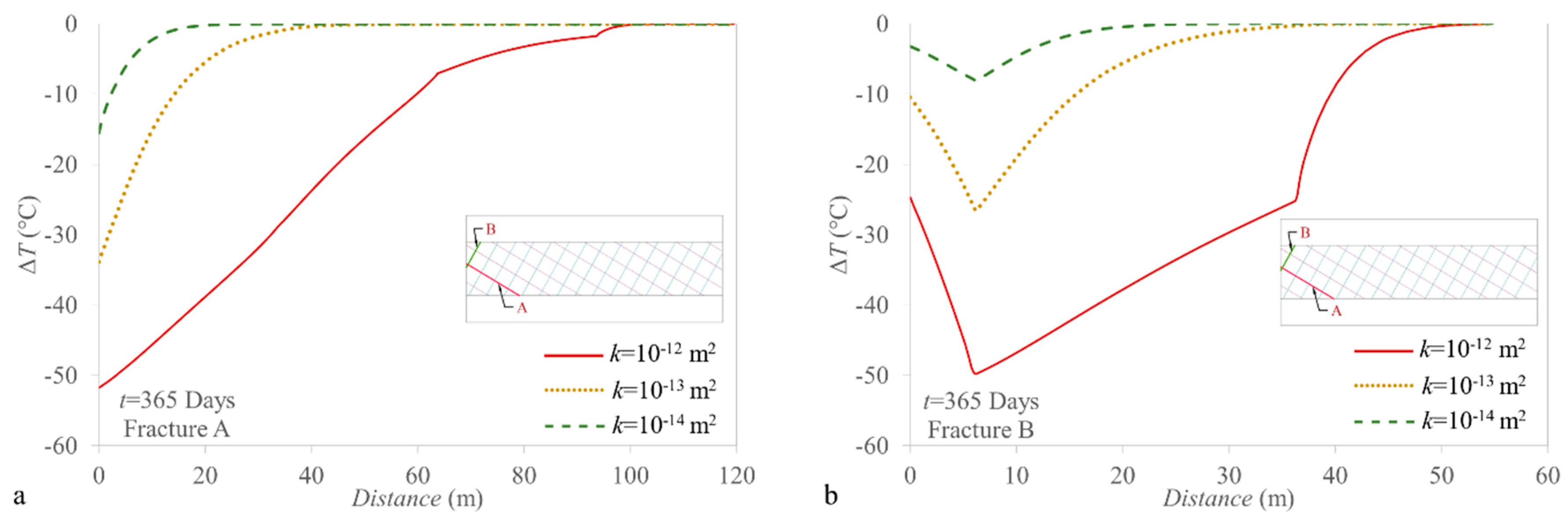
Figure 6 shows the distribution of temperature along fractures A and B. The injected low-temperature fluid moves away from the injection point through the fractures and progressively cools down the reservoir. Even though the cooling takes place rapidly within the fractures, the cooling front advances much behind than the pressure front because it has to reach thermal equilibrium with the fractures and cool down the peripheral rock matrix. Heat transfer splits at the intersection between fractures, as shown by the variation in temperature gradients within the fractures at the intersection points. CO2 injection yields a similar temperature distribution, but the cooling front advances more slowly than for water injection.
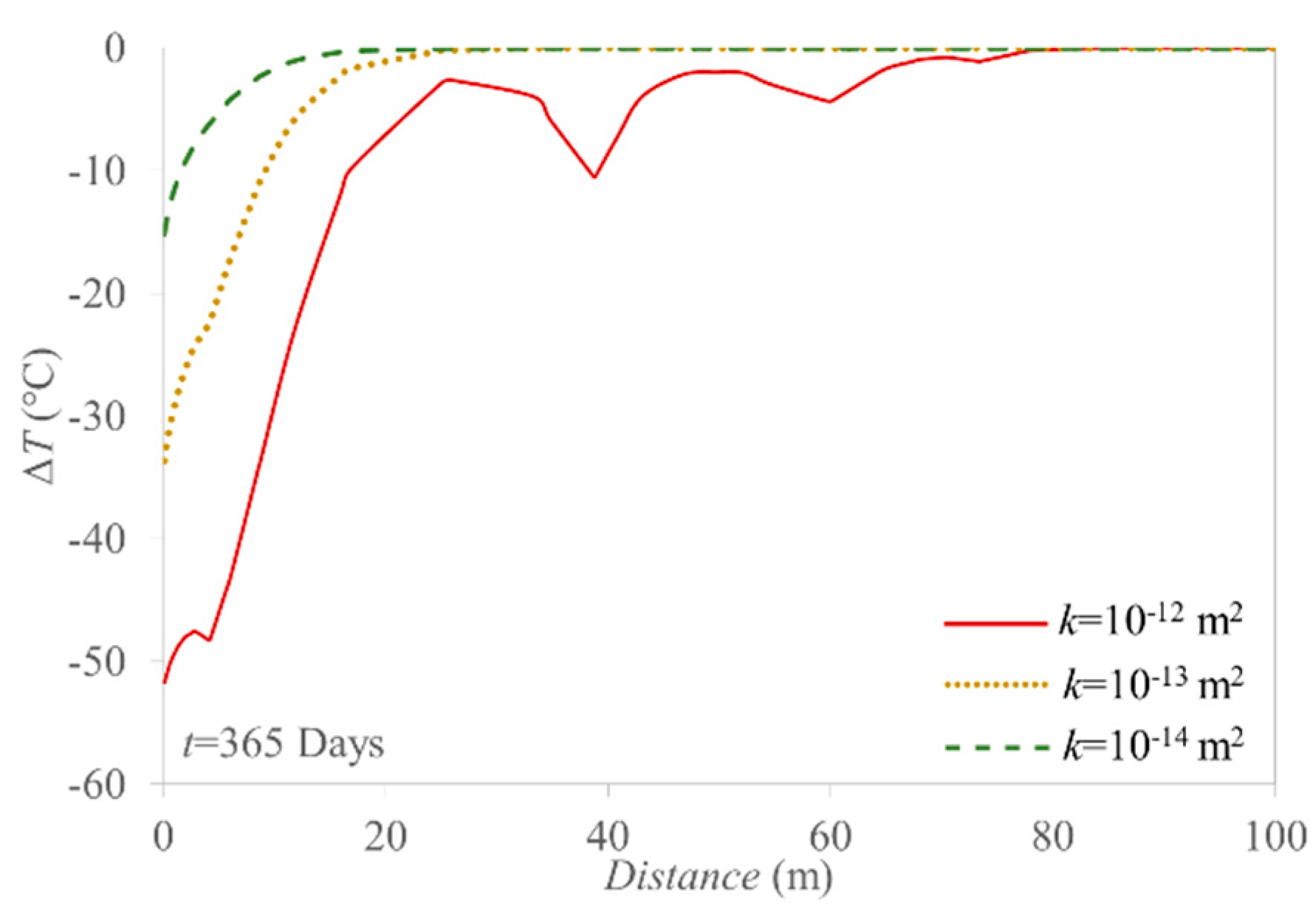
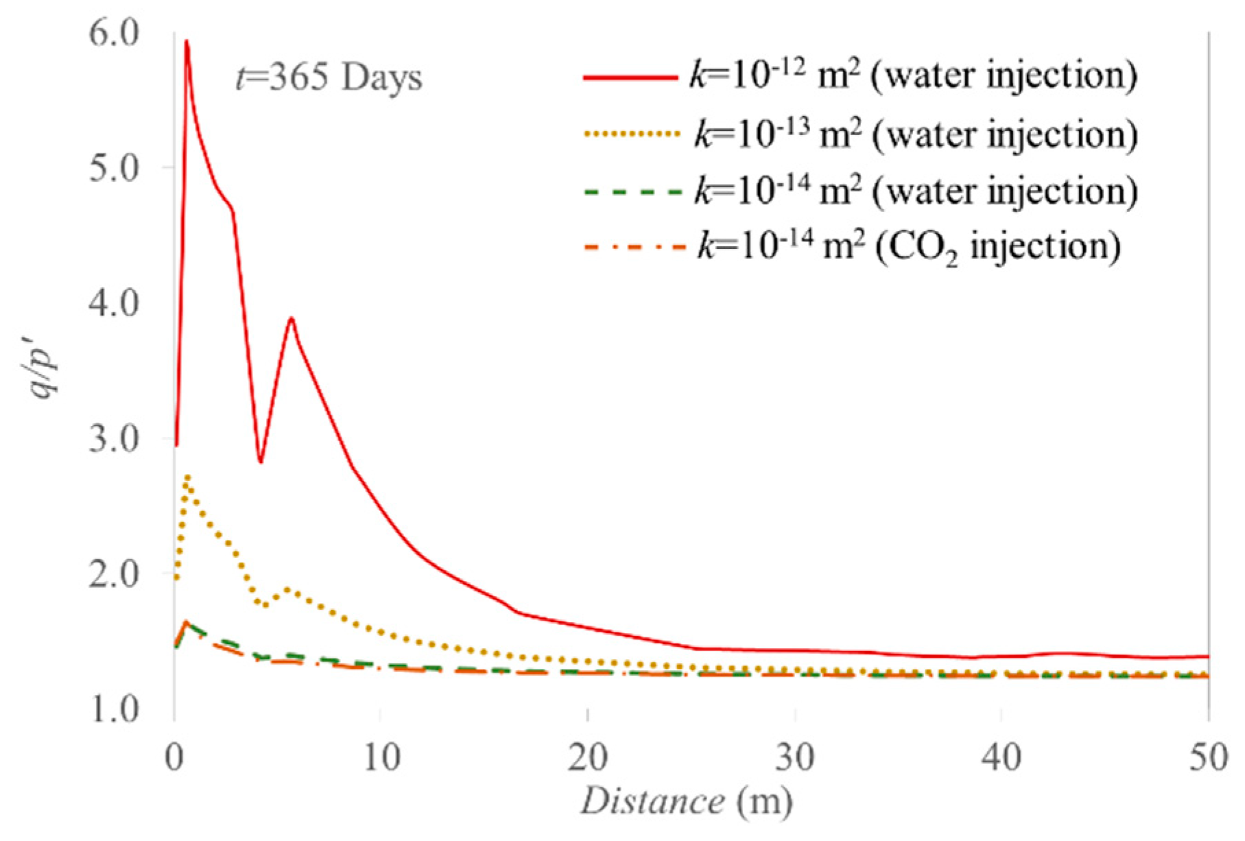
Figure 7 shows the temperature profile in the horizontal direction at the depth of the injection well. A drop in temperature is observed at the fractures position (i.e., at 4, 39, 60, and 73 m from the injection point) because cooling mainly advances through fractures by advection while the cooling of the matrix by conduction, is slower. Thus, fractures act as preferential paths of the cooling front, affecting the geomechanical response of the fractured reservoir.
3.3. Geomechanical Response
3.3.1. Stress Changes in Fractures
Simulation results show that total stresses change in response to fluid pressure variations (Figure 8), with the direct consequence that the effective stress change is lower than that of fluid pressure. This behavior, which is generally observed in HM numerical simulations [35,36,37], is not a consequence of the mechanical boundary conditions of restrained displacement, as it might be believed. Indeed, the effect of the physical constraints is very slight when the domain is sufficiently extended [38] and total stress changes are also observed in simulations with unrestrained boundaries [39]. The reason for this behavior actually lies in the hydraulic conductivity contrast between the geomaterials.
Total stress variation in response to pressure variation has been extensively analyzed for the case of horizontal thin [40,41], flat disk-shaped [42] or ellipsoidal reservoirs [43,44]. These studies consider uniform pressure distribution inside the reservoir and no diffusion toward the surrounding matrix. However, the response in the presence of a preferential flow path, like fractures or fault zones, is more complex. Indeed, the pressure distribution in the fracture is not uniform; i.e., the gradient is not equal to zero, even if the conductivity is very high. This is especially true for early times of injection.
Moreover, fractures are not completely isolated from the surrounding matrix, which undergoes a non-zero variation of pressure. Altmann et al. [45] analyzed the stress variation in response to injection in a double porosity medium and argued that the permeability contrast between the two materials sensibly affects the poromechanical response.
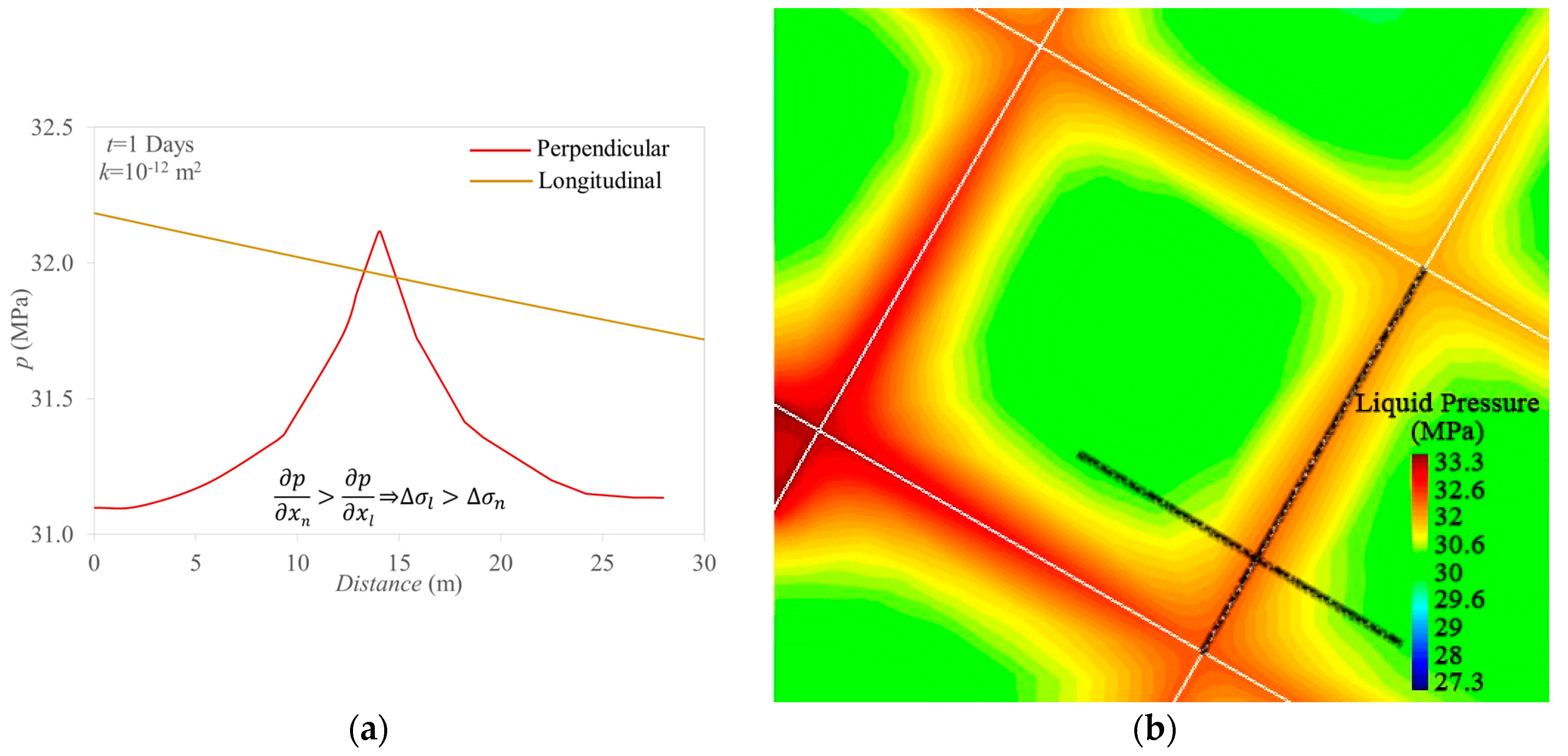
Indeed, given the difference in hydraulic parameters, pressure change mostly propagates through the more permeable fractures and barely diffuses toward the matrix. The pressure configuration shows a large and non-uniform pressure gradient in the direction normal to the fractures (Figure 8), which generates different amounts of expansion of the medium in the direction of the fracture. In particular, fractures undergo a higher expansion than the surrounding matrix. However, this differential deformation is partially hindered by the medium continuity, which leads to the total stress increase in the longitudinal direction of the fracture. A similar response is observed in thermoelasticity when a material is subject to heating or cooling [46,47].
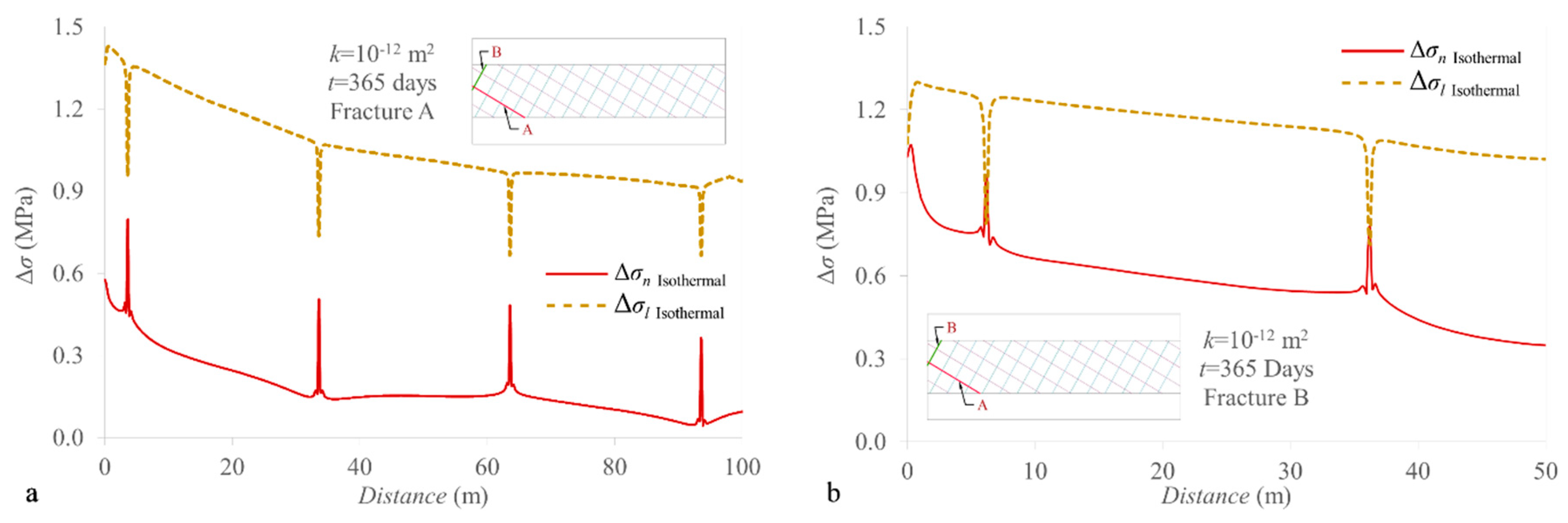
Therefore, we observe a larger increase of the total stress in the longitudinal direction of the fracture than in the direction normal to it (Figure 9), in accordance with the fact that the pressure gradient is steeper in the normal direction than in the longitudinal direction of the fracture. The abrupt changes in stress in both directions coincide with the intersection with other fractures, in which the normal and longitudinal stress changes become similar because the longitudinal direction of one fracture is the normal direction to the intersecting fracture and vice versa. The total stress variation, which arises in the pressurized portion of the fracture, is instantly transferred to the whole domain like a mechanical load.
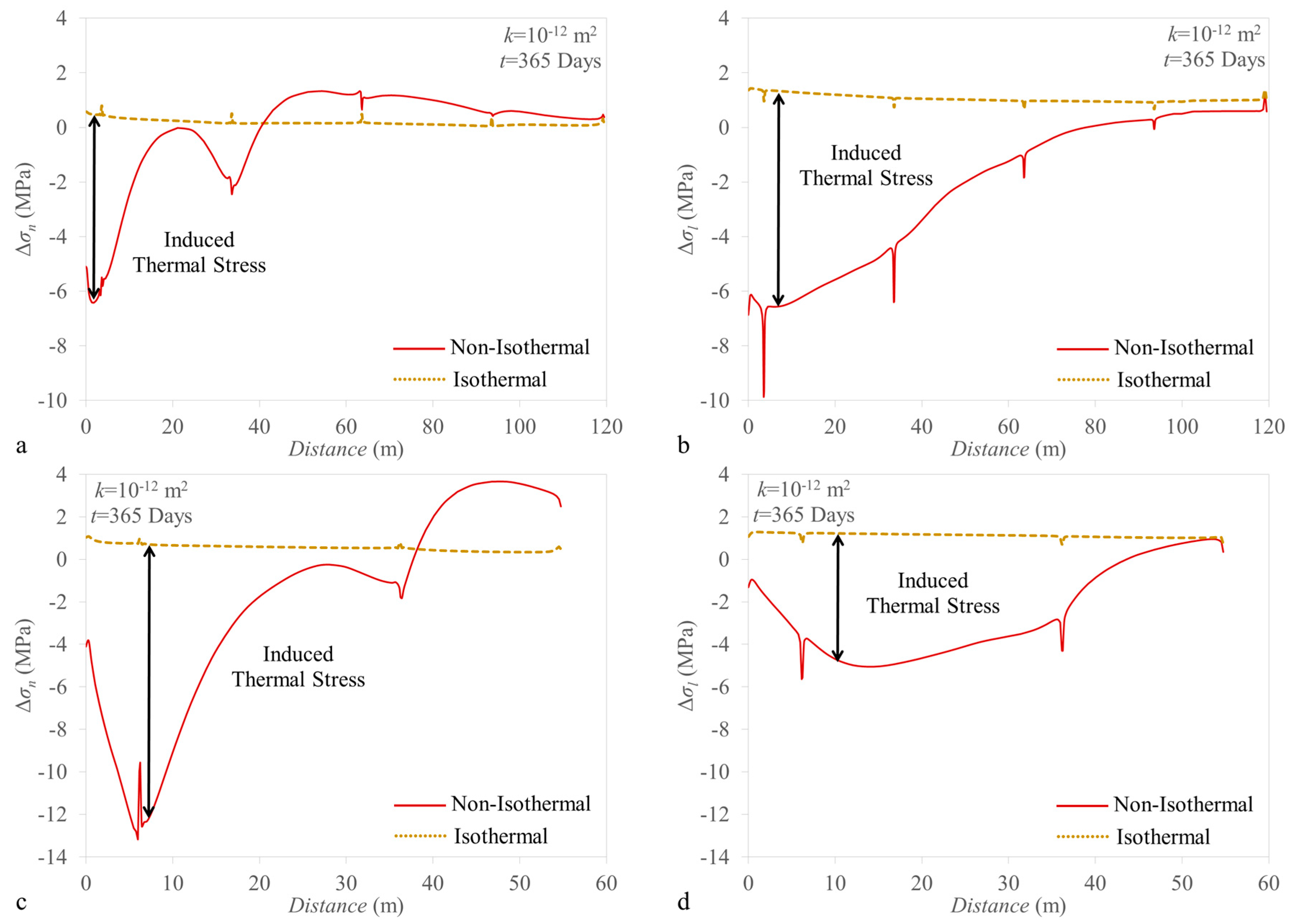
The geomechanical response to fluid flow and heat transfer are similar because both the gradients of pressure and temperature act as body forces. In fact, similarly to the response to pressure changes, we observe a large thermal stress in the longitudinal direction of the fracture with a reduction in total stress in response to temperature drop (Figure 10). However, contrary to the pressure effects, thermal stress is proportional to the material stiffness, and thus, stress variation becomes large in the portion of the matrix affected by cooling. Also, notice that in the case of thermal forcing, the variation in effective and total stresses is equal. It is worth mentioning that the spikes observed in Figure 9 and Figure 10 for both the isothermal and non-isothermal cases correspond to fractures intersections, in which the longitudinal stress in one fracture equals to the normal stress in the other fracture. But, as expected, the longitudinal stress changes are higher than those in the normal direction in the central portion of the matrix blocks.
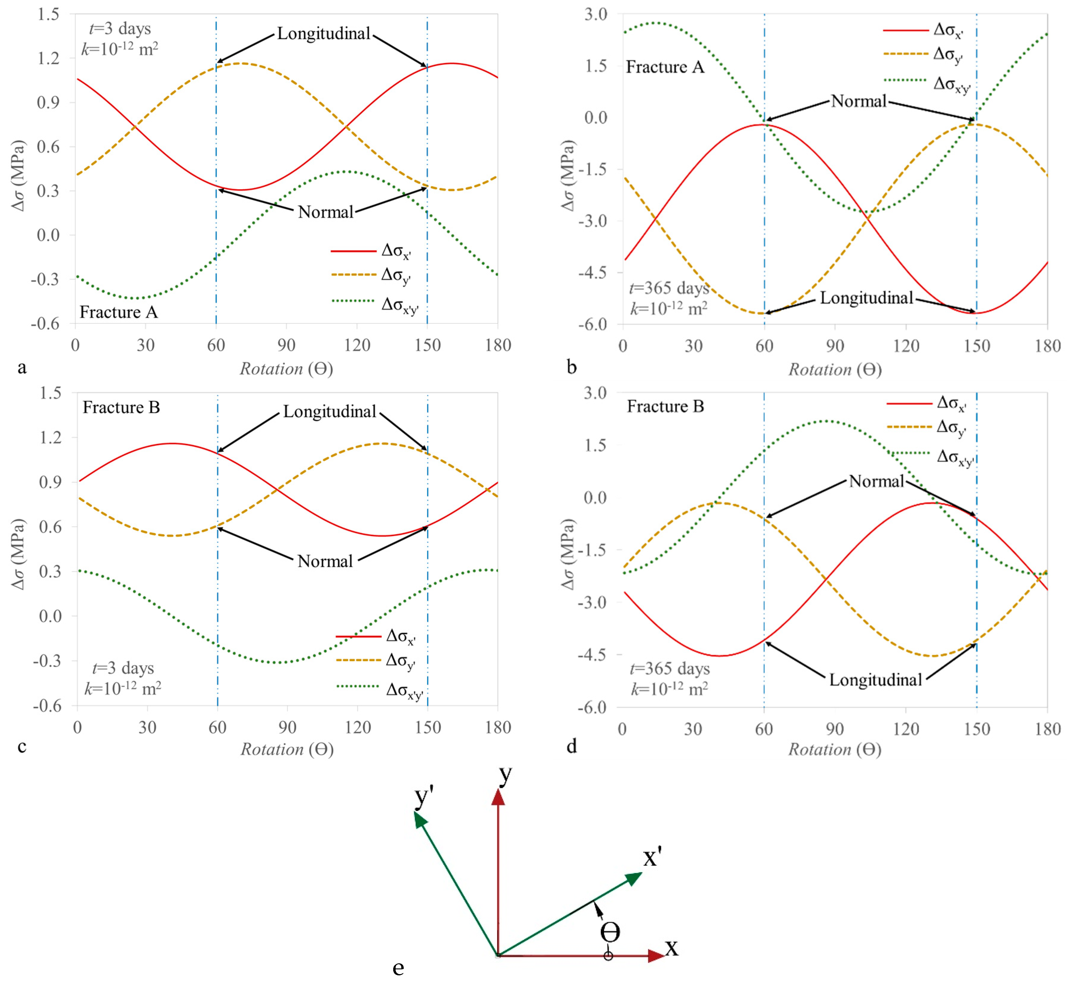
Figure 11 displays the in-plane stress changes at a point within fractures A and B as a function of orientation. For a rotation of 0°, the stress changes coincide with those of the coordinate axes; i.e., Δσx = Δσx′ and Δσy = Δσy′. In fracture A (dip of −30°), while a rotation of 60° leads Δσx′ and Δσy′ to coincide with the normal and longitudinal stresses to the fracture, respectively, a rotation of 150° leads Δσx′ and Δσy′ to coincide with the longitudinal and normal stresses to the fracture, respectively. Similarly, in fracture B, Δσx′ becomes the longitudinal stress for a rotation of 60° and the normal stress to the fracture for a rotation of 150°, and the opposite occurs for Δσy′. At the beginning of injection (day 3), cooling is negligible and only the effect of pressure buildup is observed in the fractures around the injection well (Figure 11a,c). Thus, total stresses increase as a result of pressure buildup, with the longitudinal stress change being larger than that normal to the fracture. In the long-term (1 year of injection), cooling also affects the fractures around the injection well and thus, a thermal stress reduction is induced (Figure 11b,d). Again, the total stress changes in the longitudinal direction are larger than in the normal direction to the fracture because of the difference in the pressure and temperature gradients in these directions. The maximum and minimum stress changes do not coincide with the fracture direction in all cases. This discrepancy is caused by local stress rotation around fractures induced by pressure and temperature changes and interaction between fractures.
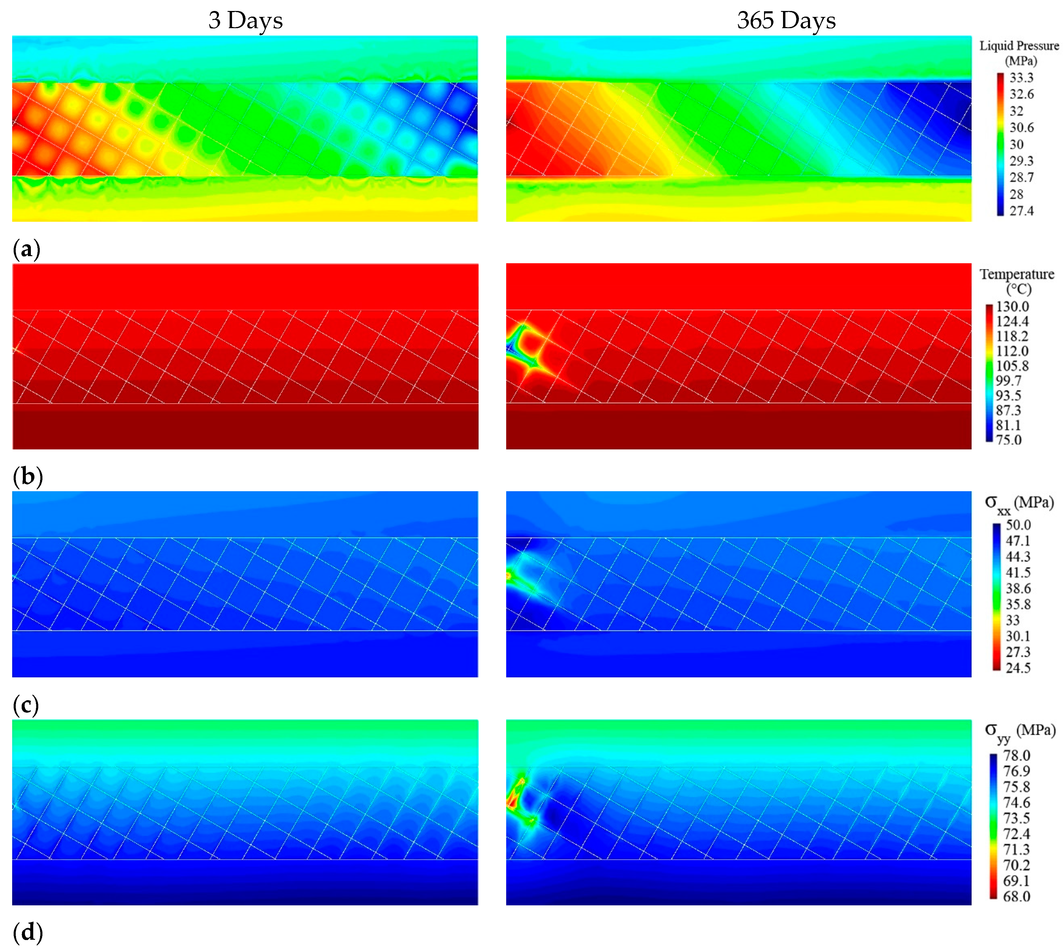
Figure 12 shows the distribution of pressure, temperature, and horizontal and vertical stresses in the short-term (3 days) and long-term (365 days) of operation for low-temperature fluid injection. At the beginning of injection, pressure diffuses through fractures causing strong pressure gradients towards the matrix blocks (Figure 12a). Eventually, the matrix blocks reach equilibrium with the pressure in the fractures, which gives rise to a homogenized pressure distribution in the long-term, when steady-state conditions have already been reached (recall Section 3.1). Cooling advances much more slowly than pressure (Figure 12b), so temperature changes are negligible in the short-term and preferentially advances through the fractures in the long-term (recall Section 3.2). These pressure and temperature variations cause changes in the total stresses (Figure 12c,d). While the main driving mechanism that changes total stresses is pressure changes in the short-term, it is cooling in the long-term. The largest total stress reduction occurs in the cooled portion of the matrix blocks because the matrix is one order of magnitude stiffer than fractures.
3.3.2. Fractures Stability
Both pressure and temperature forcing result in a non-isotropic variation of the effective stresses that affects the potential for fracture failure. Figure 13 and Figure 14 represent the stress state by means of the mean effective stress and the deviatoric stress . Prior to injection, the reservoir is stable and behaves elastically. Once injection begins, the mean effective stress and the deviatoric stress around the injection well change due to pressure buildup and temperature drop, causing an increase in the ratio. As a result, the yield envelope may be reached in some part of the reservoir, especially in the cooled region. At these parts, the rock begins to behave plastically.
Figure 13 shows that fractures A and B undergo shear failure conditions for a distance of 70 and 40 m from the injection well, respectively, if the friction angle is assumed to be of 30°; i.e., = 1.2. Simulation results show that fracture stability strongly depends on its permeability. Since shear failure is mainly driven by cooling in the modeled scenario, the lower the fracture permeability, the shorter the portion of the fracture that undergoes shear failure conditions.
Figure 14 displays the ratio along the horizontal direction from the injection point. Shear failure conditions occur within a short distance from the injection well; i.e., a maximum of 15 m. The values are significantly higher (by a factor of 2) in the matrix blocks than in the fractures (compare Figure 13 and Figure 14) because of the larger thermal stress reduction in the stiff matrix than in the soft fractures. Thus, shear fractures may be created in the matrix blocks even though its strength is higher than that of pre-existing fractures.
The changes in fracture stability are very similar regardless of the fluid that is injected; i.e., water or CO2. Nevertheless, the decrease in stability is smaller for CO2 than for water injection (Figure 13 and Figure 14). This difference is caused by the slower advance of the cooling front for CO2 injection (recall Section 3.2), which induces smaller thermal stresses.
3.3.3. Caprock Stability
Simulation results show that neither pressure nor temperature changes significantly propagate into the caprock after 1 year of operation because of the low permeability of the caprock and the slow advance of the cooling front (Figure 12). Nevertheless, fluid pressure slightly changes in the caprock as a result of the reverse water-level fluctuation (Figure 5). This pressure variations change the effective stresses in the caprock, leading to a slight decrease in stability above the injection well and a slight increase in stability above the production well. Overall, the changes in the ratio are small, which ensures a stable situation for the caprock during the operation.
4. Discussion
Fluid injection and production in NFR produces pressure changes that preferentially advance through fractures. Additionally, injected fluids are usually at a lower temperature than the reservoir, which cools down fractures and the portion of matrix blocks around them. These pressure and temperature changes cause strong gradients in the direction normal to fractures that lead to changes in the total stress in the longitudinal direction of fractures induced by the differential strain between fractures and the matrix. Consequently, the change in the effective stresses is smaller than the change in fluid pressure, which highlights the necessity to explicitly account for coupled THM processes to accurately assess fracture stability [41]. However, these effects are sometimes ignored in conventional methods by simplifications such as applying the variation of pore pressure on the effective stress state or considering equivalent porous media instead of explicitly modeling fractures.
The observed total stress changes in response to pressure changes are actually due to the permeability contrast between fractures and matrix and not to the mechanical boundary conditions. Given the difference in hydraulic parameters, fluid pressure mostly flows through the more permeable fractures, and barely diffuses toward the reservoir matrix blocks in the short-term. In the long-term, the pore pressure in the matrix blocks equilibrates with that of the fractures. Thus, the permeability contrast between fractures and the matrix sensibly affects the poromechanical response. Moreover, if there were no permeability contrast, the reservoir would become a homogeneous porous media and all the THM processes observed in this study would not take place.
Moreover, the cooling front advances due to a combination of advection and conduction in the fractures, but it only propagates by conduction into the matrix and low-permeable formations. This promotes a preferential advance of the cooling front through fractures, accentuating the larger total stress changes in the longitudinal than in the normal direction to fractures (Figure 11).
Considering cooling leads to two main differences with respect to the isothermal case. First, cooling produces a higher fluid pressure gradient as a result of the viscosity increase caused by the decrease in temperature. Second, cooling causes a decrease of the same magnitude in both total and effective stresses. The magnitude of the thermal stress change is proportional to the temperature drop and the stiffness of the rock (Equation (10)). Therefore, the thermal stress reduction is much larger in the reservoir matrix than in the fractures (Figure 12c,d).
Both pressure and temperature changes affect reservoir stability. While reservoir stability influenced by pressure changes alone can be controlled in a relatively easy way in operations in which fluid is injected and produced at a certain distance because the range of pressure perturbation can be managed during operation, cooling induced by injection of fluids may lead to reservoir instability. Such instability may occur both in the fractures and in the intact rock matrix. In the former case, pre-existing fractures would slip, inducing microseismicity, and may open up by dilation, increasing fracture permeability. In the latter case, new fractures may be formed, which would also increase reservoir permeability.
Injection in and production from NFRs rely on fractures that provide the essential porosity and permeability to the fractured reservoir. Despite providing sufficiently high permeability, the storage capacity is limited in NFRs because of the relatively high entry pressure of the matrix blocks, which maintains the injected gas (CO2) within the fractures. The relatively low storage capacity of NFRs should not prevent the implementation of CCUS projects in such reservoirs, because at the basin scale, the cumulative storage capacity becomes non-negligible, so CCUS operations can contribute to reduce CO2 emissions and obtain an economic benefit.
In this study, fractures represent high permeable discontinuities of an idealized NFR and reservoir matrix blocks represent discontinuities and intact rock with lower permeability. We have considered constant fracture permeability because we aimed at identifying the coupled THM processes that occur in a NFR. However, since fracture deformation, both elastic and irreversible, cause permeability changes, we will investigate the effects of variable permeability of fractures in future studies.
5. Conclusions
We have performed THM models to investigate the effects of cold fluid injection in a NFR. The models consider two sets of perpendicular fractures embedded into a reservoir matrix. To differentiate thermal from poromechanical effects we have compared coupled THM and HM simulations for a range of fracture intrinsic permeability. This approach facilitates understanding the simultaneous effects of pressure and temperature variations and the processes leading to induced instability in NFRs and their caprock.
The main conclusions that can be drawn from this study are:
- -
- Fluid pressure changes extend further in the fractures than in the reservoir matrix in the short-term due to the large permeability contrast between them, but pressure eventually diffuses into the matrix, leading to a homogenized pressure variation in the long-term.
- -
- The pore volume increases above the injection well and decrease above the production well in the lower part of the caprock as a result of caprock bending, causing reverse water-level fluctuations.
- -
- The permeability contrast between the fractures and the reservoir matrix causes a large and non-uniform pressure gradient in the direction normal to the fractures, which causes a greater increase of the total stress in the longitudinal direction of the fracture than in the direction normal to it.
- -
- A large thermal stress reduction occurs in the longitudinal direction of the fracture in response to temperature drop. Given that thermal stress is proportional to the material stiffness, stress reduction becomes large in the portion of the matrix affected by cooling.
- -
- Coupled THM effects in NFRs might cause local rotations of the stress tensor.
- -
- Simulations show that, after one year of operation, the cooling front does not reach the caprock, which remains stable, but the fractures and reservoir matrix close to the injection point may reach failure conditions because of thermally-induced stresses. Thus, fractures may only be reactivated around injection wells.
Author Contributions
A.Z. and V.V. conceptualized, investigated, simulated, validated, and visualized the work; A.Z. curated and analyzed the data; the methodology of the study was presented by A.Z., V.V., and S.O.; the project administration was done by A.Z.; writing the original draft was done by A.Z. and S.D.S.; reviewing and editing the work was done by A.Z., V.V., S.D.S., H.S., and S.O.; Resources were provided by V.V. and S.O.; the work was supervised by H.S. and V.V.
Acknowledgments
A.Z. acknowledges the financial support received from the “Iran’s Ministry of Science, Research and Technology” (Ph.D. students’ sabbatical grants). V.V. acknowledges financial support from the “ZoDrEx” project, which has been subsidized through the ERANET Cofund GEOTHERMICA (Project No. 731117), from the European Commission and the Spanish Ministry of Economy, Industry and Competitiveness (MINECO).
Conflicts of Interest
The authors declare no conflicts of interest.
References
- Dake, L.P. The Practice of Reservoir Engineering; Elsevier: New York, NY, USA, 2001. [Google Scholar]
- Amarnath, A. Enhanced Oil Recovery Scoping Study; Electric Power Research Institute: Palo Alto, CA, USA, 1999. [Google Scholar]
- Thomas, S. Enhanced oil recovery-an overview. Oil Gas Sci. Technol. 2008, 63, 9–19. [Google Scholar] [CrossRef]
- De Simone, S.; Vilarrasa, V.; Carrera, J.; Alcolea, A.; Meier, P. Thermal coupling may control mechanical stability of geothermal reservoirs during cold water injection. Phys. Chem. Earth 2013, 64, 117–126. [Google Scholar] [CrossRef]
- Vilarrasa, V.; Rutqvist, J.; Rinaldi, A. Thermal and Capillary effects on the caprock mechanical stability at In Salah, Algeria. Greenh. Gases Sci. Technol. 2015, 2, 408–418. [Google Scholar] [CrossRef]
- Kim, S.; Hosseini, S.A. Hydro-thermo-mechanical analysis during injection of cold fluid into a geologic formation. Int. J. Rock Mech. Min. Sci. 2015, 77, 220–236. [Google Scholar] [CrossRef] [Green Version]
- Schlumberger. Carbonate Reservoirs: Meeting Unique Challenges to Maximize Recovery. Schlumberger Mark. Anal. 2007, 1, 1–12. [Google Scholar]
- Narr, W.; Schechter, D.S.; Thompson, L.B. Naturally Fractured Reservoir Characterization; Society of Petroleum Engineers: Richardson, TX, USA, 2006. [Google Scholar]
- Nelson, R.A. Geologic Analysis of Naturally Fractured Reservoirs; Gulf Professional Pub: Houston, TX, USA, 2001. [Google Scholar]
- Tsang, C.-F. Linking Thermal, Hydrological, and Mechanical Processes in Fractured Rocks. Annu. Rev. Earth Planet. Sci. 1999, 27, 359–384. [Google Scholar] [CrossRef]
- Rutqvist, J.; Börgesson, L.; Chijimatsu, M.; Kobayashi, A.; Jing, L.; Nguyen, T.S.; Noorishad, J.; Tsang, C.F. Thermohydromechanics of partially saturated geological media: governing equations and formulation of four finite element models. Int. J. Rock Mech. Min. Sci. 2001, 38, 105–127. [Google Scholar] [CrossRef]
- Neuzil, C.E. Hydromechanical coupling in geologic processes. Hydrogeol. J. 2003, 11, 41–83. [Google Scholar] [CrossRef]
- Rutqvist, J.; Stephansson, O. The role of hydromechanical coupling in fractured rock engineering. Hydrogeol. J. 2003, 11, 7–40. [Google Scholar] [CrossRef] [Green Version]
- Rutqvist, J.; Tsang, C.-F. Multiphysics processes in partially saturated fractured rock: Experiments and models from Yucca Mountain. Rev. Geophys. 2012, 50. [Google Scholar] [CrossRef] [Green Version]
- Vilarrasa, V.; Rutqvist, J. Thermal effects on geologic carbon storage. Earth Sci. Rev. 2017, 165, 245–256. [Google Scholar] [CrossRef] [Green Version]
- Wang, W.; Kolditz, O. Object-oriented finite element analysis of thermo-hydro-mechanical (THM) problems in porous media. Int. J. Numer. Methods Eng. 2007, 69, 162–201. [Google Scholar] [CrossRef]
- Börgesson, L. ABAQUS. Dev. Geotech. Eng. 1996, 79, 565–570. [Google Scholar]
- Israelsson, J.I. Short description of FLAC version 3.2. Dev. Geotech. Eng. 1996, 79, 513–522. [Google Scholar]
- Israelsson, J.I. Short Descriptions of UDEC and 3DEC. Dev. Geotech. Eng. 1996, 79, 523–528. [Google Scholar]
- Olivella, S.; Carrera, J.; Gens, A.; Alonso, E.E. Nonisothermal multiphase flow of brine and gas through saline media. Transp. Porous Media 1994, 15, 271–293. [Google Scholar] [CrossRef]
- Olivella, S.; Gens, A.; Carrera, J.; Alonso, E.E. Numerical formulation for a simulator (CODE_BRIGHT) for the coupled analysis of saline media. Eng. Comput. 1996, 13, 87–112. [Google Scholar] [CrossRef] [Green Version]
- Pan, P.-Z.; Rutqvist, J.; Feng, X.-T.; Yan, F. Modeling of caprock discontinuous fracturing during CO2 injection into a deep brine aquifer. Int. J. Greenh. Gas Control 2013, 19, 559–575. [Google Scholar] [CrossRef]
- Pan, P.-Z.; Rutqvist, J.; Feng, X.-T.; Yan, F. An Approach for Modeling Rock Discontinuous Mechanical Behavior Under Multiphase Fluid Flow Conditions. Rock Mech. Rock Eng. 2014, 47, 589–603. [Google Scholar] [CrossRef]
- Hubbert, M.K. Darcy’s Law and the Field Equations of the Flow of Underground Fluid. Int. Assoc. Sci. Hydrol. Bull. 1956, 2, 23–59. [Google Scholar] [CrossRef]
- Bear, J. Dynamics of Fluids in Porous Media; Courier Corporation: Chelmsford, MA, USA, 1972. [Google Scholar]
- Olivella, S.; Alonso, E.E. Gas flow through clay barriers. Géotechnique 2008, 58, 157–176. [Google Scholar] [CrossRef] [Green Version]
- Witherspoon, P.A.; Wang, J.S.Y.; Iwai, K.; Gale, J.E. Validity of Cubic Law for fluid flow in a deformable rock fracture. Water Resour. Res. 1980, 16, 1016–1024. [Google Scholar] [CrossRef] [Green Version]
- Nield, D.A.; Bejan, A. Convection in Porous Media; Springer: Berlin, Germany, 2017. [Google Scholar]
- Biot, M.A. Thermoelasticity and irreversible thermodynamics. J. Appl. Phys. 1956, 27, 240–253. [Google Scholar] [CrossRef]
- Mctigue, D.F. Thermoelastic Response of Fluid-Saturated Porous Rock. J. Geophys. Res. 1986, 91, 9533–9542. [Google Scholar] [CrossRef]
- Vilarrasa, V.; Rinaldi, A.P.; Rutqvist, J. Long-term thermal effects on injectivity evolution during CO2 storage. Int. J. Greenh. Gas Control 2017, 64, 314–322. [Google Scholar] [CrossRef]
- Hsieh, P.A. Deformation-Induced Changes in Hydraulic Head During Ground-Water Withdrawal. Ground Water 1996, 34, 1082–1089. [Google Scholar] [CrossRef]
- Kim, J.-M.; Parizek, R.R. Numerical simulation of the Noordbergum effect resulting from groundwater pumping in a layered aquifer system. J. Hydrol. 1997, 202, 231–243. [Google Scholar] [CrossRef]
- Vilarrasa, V.; Carrera, J.; Olivella, S. Hydromechanical characterization of CO2 injection sites. Int. J. Greenh. Gas Control 2013, 19, 665–677. [Google Scholar] [CrossRef]
- Rutqvist, J.; Birkholzer, J.T.; Tsang, C.F. Coupled reservoir-geomechanical analysis of the potential for tensile and shear failure associated with CO2 injection in multilayered reservoir-caprock systems. Int. J. Rock Mech. Min. Sci. 2008, 45, 132–143. [Google Scholar] [CrossRef]
- Vilarrasa, V.; Bolster, D.; Olivella, S.; Carrera, J. Coupled hydromechanical modeling of CO2 sequestration in deep saline aquifers. Int. J. Greenh. Gas Control 2010, 4, 910–919. [Google Scholar] [CrossRef] [Green Version]
- Jeanne, P.; Rutqvist, J.; Dobson, P.F.; Walters, M.; Hartline, C.; Garcia, J. The impacts of mechanical stress transfers caused by hydromechanical and thermal processes on fault stability during hydraulic stimulation in a deep geothermal reservoir. Int. J. Rock Mech. Min. Sci. 2014, 72, 149–163. [Google Scholar] [CrossRef]
- De Simone, S.; Carrera, J.; Vilarrasa, V. Superposition approach to understand triggering mechanisms of post-injection induced seismicity. Geothermics 2017, 70, 85–97. [Google Scholar] [CrossRef]
- De Simone, S.; Carrera, J.; Gómez-Castro, B.M. A practical solution to the mechanical perturbations induced by non-isothermal injection into a permeable medium. Int. J. Rock Mech. Min. Sci. 2017, 91, 7–17. [Google Scholar] [CrossRef]
- Engelder, T.; Fischer, M.P. Influence of poroelastic behavior on the magnitude of minimum horizontal stress, Sh in overpressured parts of sedimentary basins. Geology 1994, 22, 949–952. [Google Scholar] [CrossRef]
- Hillis, R. Pore pressure/stress coupling and its implications for seismicity. Explor. Geophys. 2000, 31, 448–454. [Google Scholar] [CrossRef]
- Geertsma, J. Land Subsidence above Compacting Oil and Gas Reservoirs. J. Pet. Technol. 1973, 25, 734–744. [Google Scholar] [CrossRef]
- Segall, P.; Fitzgerald, S.D. A note on induced stress changes in hydrocarbon and geothermal reservoirs. Tectonophysics 1998, 289, 117–128. [Google Scholar] [CrossRef]
- Rudnicki, J.W. Alteration of Regional Stress by Reservoirs and other Inhomogeneities: Stabilizing or Destabilizing? In Proceedings of the 9th ISRM Congress, Paris, France, 25–28 August 1999. [Google Scholar]
- Altmann, J.B.; Müller, T.M.; Müller, B.I.R.; Tingay, M.R.P.; Heidbach, O. Poroelastic contribution to the reservoir stress path. Int. J. Rock Mech. Min. Sci. 2010, 47, 1104–1113. [Google Scholar] [CrossRef] [Green Version]
- Timoshenko, S.; Goodier, J.N. Theory of Elasticity; McGraw-Hill: New York, NY, USA, 1970. [Google Scholar]
- Boley, B.A. Theory of Thermal Stresses; Dover Publications: Mineola, NY, USA, 2012. [Google Scholar]
Figure 1.
Schematic description of the model geometry and boundary conditions.

Figure 2.
Fluid pressure changes along the fractures with different dips as a function of the distance, (a) fracture A (dip −30°) and (b) fracture B (dip 60°). Note that the changes in the pressure gradient coincide with intersections with other fractures.
Figure 2.
Fluid pressure changes along the fractures with different dips as a function of the distance, (a) fracture A (dip −30°) and (b) fracture B (dip 60°). Note that the changes in the pressure gradient coincide with intersections with other fractures.

Figure 3.
Fluid pressure changes along the horizontal direction in the reservoir (a) after 3 days of injection and (b) after 1 year of injection. Note that the fluctuations are due to the larger pressure changes that occur in the fractures with respect to the reservoir matrix.
Figure 3.
Fluid pressure changes along the horizontal direction in the reservoir (a) after 3 days of injection and (b) after 1 year of injection. Note that the fluctuations are due to the larger pressure changes that occur in the fractures with respect to the reservoir matrix.

Figure 4.
Distribution of liquid saturation degree for low-temperature CO2 injection after 365 days of injection and production for fractures with intrinsic permeability of 10−14 m2.
Figure 4.
Distribution of liquid saturation degree for low-temperature CO2 injection after 365 days of injection and production for fractures with intrinsic permeability of 10−14 m2.

Figure 5.
Liquid pressure during a 1-year injection and production period for a point at the bottom of the caprock placed 1.5 m above the reservoir-caprock interface and 30 m away from (a) the injection boundary and (b) the production boundary.
Figure 5.
Liquid pressure during a 1-year injection and production period for a point at the bottom of the caprock placed 1.5 m above the reservoir-caprock interface and 30 m away from (a) the injection boundary and (b) the production boundary.

Figure 6.
Temperature evolution along the fractures near to the injection point when fluid is injected 50 °C cooler than the reservoir temperature during 1 year, for (a) fracture A and (b) fracture B.
Figure 6.
Temperature evolution along the fractures near to the injection point when fluid is injected 50 °C cooler than the reservoir temperature during 1 year, for (a) fracture A and (b) fracture B.

Figure 7.
Temperature distribution along the horizontal line from the injection point after 1-year of injection.
Figure 7.
Temperature distribution along the horizontal line from the injection point after 1-year of injection.

Figure 8.
(a) Pressure gradient in the longitudinal (xl) and normal (xn) directions of a fracture after 1 day of injection and (b) fluid pressure distribution due to injection into a fractured medium and sections depicted in the profiles shown in (a). Note that pressure buildup mostly propagates into the longitudinal direction of a fracture. Consequently, the pressure gradient in the normal direction is greater than in the longitudinal direction.

Figure 9.
Total stress changes in the normal and longitudinal directions for isothermal injection along fractures (a) A and (b) B after 1 year of injection for a fracture with intrinsic permeability of 10−12 m2.
Figure 9.
Total stress changes in the normal and longitudinal directions for isothermal injection along fractures (a) A and (b) B after 1 year of injection for a fracture with intrinsic permeability of 10−12 m2.

Figure 10.
(a) Normal stress change along fracture A, (b) longitudinal stress change along fracture A, (c) normal stress change along fracture B and (d) longitudinal stress change along fracture B after 1 year of cold fluid injection for a fracture with intrinsic permeability of 10−12 m2.
Figure 10.
(a) Normal stress change along fracture A, (b) longitudinal stress change along fracture A, (c) normal stress change along fracture B and (d) longitudinal stress change along fracture B after 1 year of cold fluid injection for a fracture with intrinsic permeability of 10−12 m2.

Figure 11.
Stress rotations in two points on fractures A and B in response to thermal-hydro-mechanical (THM) effects for intrinsic permeability equal to 10−12 m2 (a) for fracture A, after 3 days of injection, (b) for fracture A, after 365 days of injection, (c) for fracture B, after 3 days of injection, (d) for fracture B, after 365 days of injection and (e) schematic representation of the reference axes for a rotation angle ϴ.

Figure 12.
Distribution of (a) liquid pressure, (b) temperature, (c) horizontal total stresses, and (d) vertical total stress for low-temperature fluid injection after 3 and 365 days of injection and production for fractures with intrinsic permeability of 10−12 m2.
Figure 12.
Distribution of (a) liquid pressure, (b) temperature, (c) horizontal total stresses, and (d) vertical total stress for low-temperature fluid injection after 3 and 365 days of injection and production for fractures with intrinsic permeability of 10−12 m2.

Figure 13.
trajectory along the fractures near to the injection point when cold water or CO2 are injected during 1 year, for (a) fracture A and (b) fracture B. Note that the fluctuations indicate the intersections between fractures.
Figure 13.
trajectory along the fractures near to the injection point when cold water or CO2 are injected during 1 year, for (a) fracture A and (b) fracture B. Note that the fluctuations indicate the intersections between fractures.

Figure 14.
trajectory in the horizontal direction at the depth of the injection point when cold water or CO2 are injected during 1 year. Note that the internal friction angle of the reservoir matrix is higher than that of pre-existing fractures and thus, the failure thresholds are different in fractures and reservoir matrix.


Table 1.
Material properties used in the thermo-hydro-mechanical analysis of the naturally fractured reservoirs (NFR).
Table 1.
Material properties used in the thermo-hydro-mechanical analysis of the naturally fractured reservoirs (NFR).
| Parameters | Units | Reservoir | Cap and Base Rocks | |
|---|---|---|---|---|
| Fractures | Matrix | |||
| Young’s modulus | GPa | 1.2 | 12.0 | 4.0 |
| Poisson ratio | - | 0.25 | 0.25 | 0.25 |
| Intrinsic permeability | m2 | 10−12–10−14 | 10−17 | 10−20 |
| Relative permeability | - | |||
| Entry pressure | MPa | 0.01 | 0.1 | 5 |
| Porosity | % | 15 | 15 | 5 |
| Thermal conductivity | Wm−1K−1 | 2.0 | 2.0 | 1.5 |
| Linear thermal expansion | 10−5/°C | 3.0 | 3.0 | 2.0 |
| Specific heat for solid phase | 103 J/kg K | 1 | 1 | 1 |
| Longitudinal dispersity for heat | m | 10 | 10 | 10 |
| Transversal dispersity for heat | m | 1 | 1 | 1 |
© 2018 by the authors. Licensee MDPI, Basel, Switzerland. This article is an open access article distributed under the terms and conditions of the Creative Commons Attribution (CC BY) license (http://creativecommons.org/licenses/by/4.0/).
Share and Cite
MDPI and ACS Style
Zareidarmiyan, A.; Salarirad, H.; Vilarrasa, V.; De Simone, S.; Olivella, S. Geomechanical Response of Fractured Reservoirs. Fluids 2018, 3, 70. https://doi.org/10.3390/fluids3040070
AMA Style
Zareidarmiyan A, Salarirad H, Vilarrasa V, De Simone S, Olivella S. Geomechanical Response of Fractured Reservoirs. Fluids. 2018; 3(4):70. https://doi.org/10.3390/fluids3040070
Chicago/Turabian StyleZareidarmiyan, Ahmad, Hossein Salarirad, Victor Vilarrasa, Silvia De Simone, and Sebastia Olivella. 2018. "Geomechanical Response of Fractured Reservoirs" Fluids 3, no. 4: 70. https://doi.org/10.3390/fluids3040070