
Remote Sensing of the Subtropical Front in the Southeast Pacific and the Ecology of Chilean Jack Mackerel Trachurus murphyi


College of Marine Science and Technology, Zhejiang Ocean University, Zhoushan 316022, China
*
Author to whom correspondence should be addressed.
Fishes 2023, 8(1), 29; https://doi.org/10.3390/fishes8010029
Submission received: 5 December 2022
/
Revised: 23 December 2022
/
Accepted: 26 December 2022
/
Published: 2 January 2023
(This article belongs to the Special Issue Application of Remote Sensing in Fisheries)
Abstract
:The Subtropical Front (STF) plays a key role in the ecology of Chilean jack mackerel Trachurus murphyi. Nonetheless, there are few remote sensing studies of the STF in the open Southeast Pacific, and almost all of them have been conducted by satellite oceanographers in Russia and Ukraine to support respective large-scale fisheries of jack mackerel in this region. We reviewed these studies that documented long-term seasonal and interannual variability of the STF from sea surface temperature (SST) and sea surface height (SSH) data. We also mapped the STF from satellite sea surface salinity (SSS) data of the SMOS mission (2012–2019). The Subtropical Front consists of two fronts–North and South STF about 500 km apart–that border the Subtropical Frontal Zone (STFZ) in-between. The STF is density-compensated, with spatially divergent manifestations in temperature and salinity. In the temperature field, the STF extends in the WNW to ESE direction in the Southeast Pacific. In the salinity field, the STFZ appears as a broad frontal zone, extending zonally across the entire South Pacific. Three major types of satellite data-SST, SSH, and SSS-can be used to locate the STF. The SSH data is most advantageous with regard to the jack mackerel fisheries, owing to the all-weather capability of satellite altimetry and the radical improvement of the spatial resolution of SSH data in the near future. Despite the dearth of dedicated in situ studies of the South Pacific STFZ, there is a broad consensus regarding the STFZ being the principal spawning and nursing ground of T. murphyi and a migration corridor between Chile and New Zealand. Major data/knowledge gaps are identified, and key next steps are proposed to mitigate the data/knowledge gaps and inform fisheries management.
1. Introduction
The subtropical-subantarctic belt of the South Pacific, especially its central part between 30° S and 45° S, is the least studied region of the World Ocean. The extreme remoteness of this area challenged sea-going oceanographers before the advent of satellite oceanography. Meanwhile, this region became a major fishing ground after a discovery in the 1970s of an abundant population of Chilean jack mackerel Trachurus murphyi. Catches of T. murphyi in the South Pacific reached 5 Mt by 1995—a huge number given the total global fish catch of 100 Mt at the time. Clearly, the 5 Mt/year catch was unsustainable. As a result of overfishing and poor recruitment, exacerbated by complex interactions between fishing, climate, and stock dynamics, the jack mackerel fishery collapsed [1]. Now this fishery is tightly regulated, owing in a large part to the creation of the South Pacific Regional Fisheries Management Organisation (SPRFMO). Once fully recovered, the jack mackerel fishery will become one of the world’s most important sustainable deep-sea fisheries. The protection and conservation of this valuable resource provides a strong impetus for marine ecology studies.
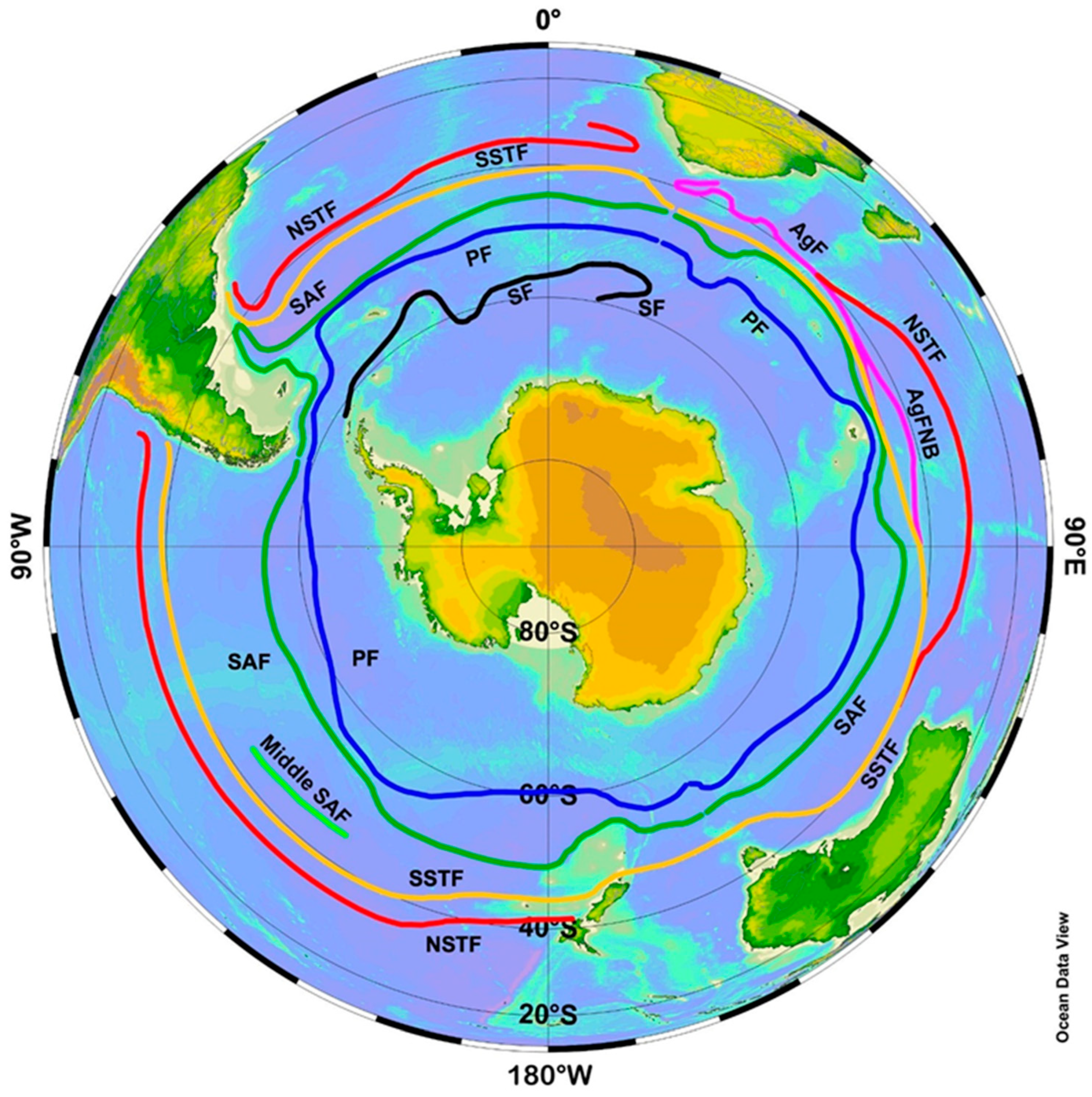
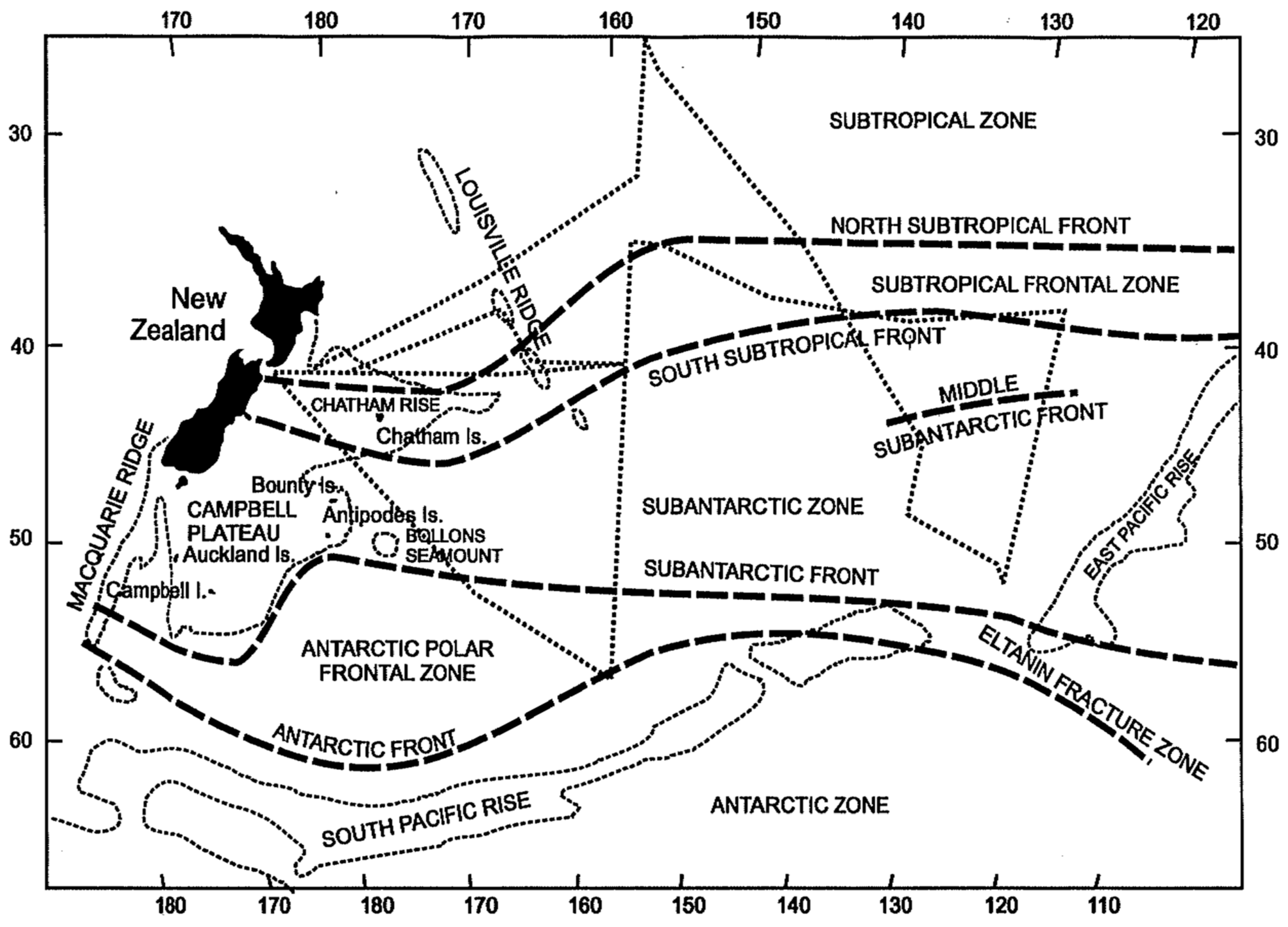
The main oceanographic feature of this region is the Subtropical Front (STF) associated with the South Pacific Current and extended WSW-ENE across the entire South Pacific as reported by Stramma et al. [2] from hydrographic section data. Belkin [3] documented the STF in the South Pacific between New Zealand and 126° W, where the STF was found to consist of two parallel fronts 400–500 km apart, termed the North and South STF (NSTF and SSTF, respectively), that border the subtropical frontal zone (STFZ) in-between. In a follow-up study, Belkin [4] identified a similar STFZ in the South Atlantic. Finally, when Belkin and Gordon [5] discovered the North STF in the South Indian Ocean, the concept of a circumpolar STFZ in the Southern Ocean was born (Figure 1, modified from ([5], Figure 5) using the Ocean Data View (ODV) software by Schlitzer [6]).
The STFZ is well observed in the Southwest Pacific, between Tasmania and the Chatham Islands. By contrast, very few oceanographic expeditions explored the STFZ east of the Chatham Islands, across the central South Pacific, up to the Southeast Pacific, where ocean fronts were systematically studied by Chilean scientists, largely in a series of papers by Chaigneau and Pizarro [7,8,9]. The central South Pacific, far from the shores of New Zealand and Chile, is prohibitively remote, which explains why the data coverage of the STFZ is sparse.
In the west, the spatial density of CTD data drops off precipitously east of the Chatham Islands. In the east, the CTD data density drops off west of 100° W–110° W. Thus, the vast area between 175° W and 110° W is data poor. The western and central parts of this area, between New Zealand and 126° W, were covered by a large-scale oceanographic survey during the R/V Dmitriy Mendeleyev Cruise 34 [3,10,11,12]. This survey, conducted in early 1985, remains the only dedicated multi-disciplinary oceanographic study of the Central South/Southeast Pacific to date. In the 1990s–2000s, high-quality CTD data were acquired during the World Ocean Circulation Experiment (WOCE) when a few meridional CTD sections were occupied across the South Pacific STFZ, including the Southeast Pacific [13,14]. Nonetheless, the in-situ data coverage of the STFZ region remains sparse to date. The dearth of quality in-situ data explains why no review of the South Pacific STFZ was ever attempted. The paucity of in-situ data was partly mitigated by remote sensing from satellites. The availability of satellite data that lends itself to mapping the STFZ was the main impetus for the remote sensing studies reviewed in this paper.
Another strong motivation for this work was the need to elucidate relations between the STFZ and ecology of Chilean jack mackerel Trachurus murphyi. In general, the ecological importance of the Southern Ocean STFZ has been widely recognized [15,16]. In particular, the spatial association between the STF/STFZ and Chilean jack mackerel was recognized early on [17,18]. Nonetheless, the role played by the South Pacific STFZ in the ecology of T. murphyi has not been emphasized in numerous ecological and fisheries oceanography studies (reviewed, among others, by Gerlotto and Dioses [19]). In many studies of T. murphyi, the South Pacific STFZ and its role were simply ignored. The present review is an attempt to rectify this situation.
2. Data and Methods
The majority of remote sensing studies of the central and eastern parts of the South Pacific STFZ were conducted in Russia and Ukraine and published almost exclusively in Russian. While the extreme westernmost and easternmost sectors were covered by studies conducted, respectively, in New Zealand and Chile, the vast swath of the South Pacific between the respective EEZs has not been a subject of peer-reviewed remote sensing studies by other countries except Russia and Ukraine. The present review is focused on this valuable information resource, which to date has remained largely untapped by the international community.
Systematic processes for reviews, such as systematic maps, are now commonplace and the gold standard for reviews; therefore, the below description follows the formalism proposed by Haddaway et al. [20], including a certain structure (systematic map protocols or checklists) for descriptions of metadata (https://www.roses-reporting.com/systematic-map-protocols; accessed 4 December 2022).
Our search strategy was comprehensive and inclusive owing to several factors. First, the search focused on a single geographic region (open South Pacific). Second, the search focused on a single oceanic feature (Subtropical Front). Third, the open South Pacific is prohibitively remote, so that every publication is eminently valuable and should not be excluded. Fourth, the search focused on papers published by only two countries (Russia and Ukraine) since other countries have not conducted academic studies of this most remote region of the World Ocean (save for a few long oceanographic sections under the aegis of the World Ocean Circulation Experiment, WOCE). Fifth, the search was performed in two languages (Russian and English; most papers by Ukrainian researchers were published in Russian). Sixth, oceanographic data collected by the fishing industry remain largely proprietary and do not appear in publicly available reports.
Scopus was our main search engine and also a de facto bibliographic database. Before switching to Scopus in 2018, we used Web of Science (WOS) for many years. Google Scholar was used as an alternative search engine. Russian-language papers were accessed online via two scientific libraries in Russia: e-Library (https://www.elibrary.ru/defaultx.asp; accessed 4 December 2022) and CyberLeninka (https://cyberleninka.ru/; accessed 4 December 2022), the latter being an Open Science library.
To ensure the reproducibility of our work, we (1) limited our survey to those sources that are freely available online at no charge, (2) provided DOI or URL for every source; (3) hyper-linked all sources in Section 3 to respective references. Our Boolean search terms are listed in Keywords.
We searched all available English-language literature published in peer-reviewed international journals and SPRFMO reports. We accessed websites with online archives of scientific publications, including the main Russian fisheries oceanography institute, VNIRO (Moscow), and its regional branches in Kaliningrad (AtlantNIRO), Vladivostok (TINRO), and Kerch (Ukraine, YugNIRO). A few Russian periodicals have recently made their PDF archives of published papers freely accessible on the Web, particularly Trudy VNIRO, whose entire PDF archive since Vol. 1 (published in 1935) is now available at http://www.vniro.ru/en/scientificactivities/publishingvniro/bulletins/trudy-vniro; other notable periodicals include Izvestiya TINRO (https://izvestiya.tinro-center.ru/jour) and Trudy AtlantNIRO (http://atlant.vniro.ru/index.php/trudy-atlantniro/vypuski-zhurnala) (both accessed 4 December 2022).
The Russian and Ukrainian satellite oceanography papers (Table 1) constitute the only massive information source on this region to date. The main goal of these studies was to provide an oceanographic background for Russian and Ukrainian fisheries of Chilean jack mackerel Trachurus murphyi. The Russian and Ukrainian remote sensing studies of the South Pacific STFZ began in the 2000s, long after the collapse of the T. murphyi fisheries in the 1990s. A few research groups have been active at the same time, located in Moscow, St. Petersburg, and Kaliningrad in Russia and Sevastopol in Ukraine. These groups used a similar approach to front detection. We searched respective papers and other relevant sources from the advent of satellite oceanography in the late 1970s and up to December 2022.
3. Satellite Oceanography of the Subtropical Front in the Southeast Pacific
The below literature survey proceeds chronologically and includes all satellite oceanography papers on this region that are freely accessible on the Web to date (December 2022). No effort was spared to make this survey truly comprehensive; therefore, any omission is not intentional.
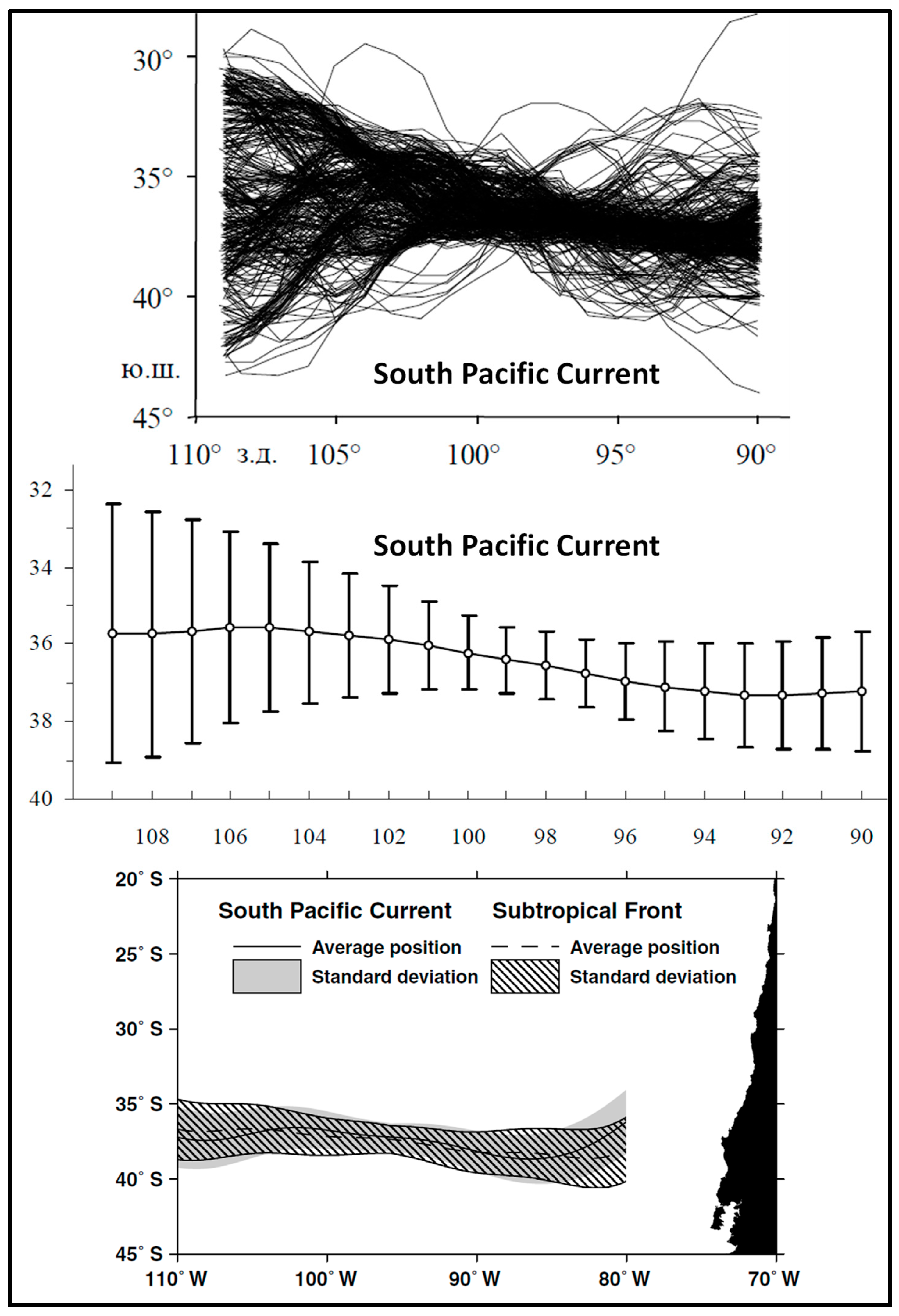
Sirota et al. [28] mapped the South Pacific Current (SPC) as the locus of maximum gradients of dynamic topography (SSH), leaving aside the thorny issue of discrepancy between the locations of STF determined from hydrographic data (temperature and salinity) vs. those determined from SSH data (so-called “dynamic STF” [29]). The discrepancy between the hydrographic STF and dynamic STF is caused by the density-compensated nature of the STF [2,30]. Sirota et al. [28] used SSH data from the TOPEX/Poseidon satellite altimetry mission in 1992–2003 to map maximum SSH gradients in the Southeast Pacific (Figure 2, top and middle panels). The SPC was found to be nearly zonal between 109° W and 90° W, with a slight non-zonal spatial trend from 36° S in the west to 37° S in the east, across the study area. The slight deviation of the SPC from a strictly zonal trend contrasts with the distinct WNW–ESE trend of the STF determined from SST data and described below. The relative stability (variability minimum) of the STC path around 100° W noted by Sirota et al. [28] is also collocated with maximum meridional gradients of SSH, hence maximum eastward geostrophic currents.
In a follow-up study, Lebedev and Sirota [26] expanded the study area eastward up to 80° W (Figure 2, bottom panel). In addition to mapping the SPC from the TOPEX/Poseidon SSH data (1992–2003), they mapped the STF from multi-channel SST data, MCSST. In both cases, the SPC and STF paths are nearly zonal and close to one another. The northward bend of the SPC east of 85° W is caused by the topographic deflection owing to the proximity of the South American continent. The nearly zonal path of STF determined by Lebedev and Sirota [26] from MCSST is inconsistent with the strongly non-zonal path of STF in the same area determined by other researchers as discussed below.
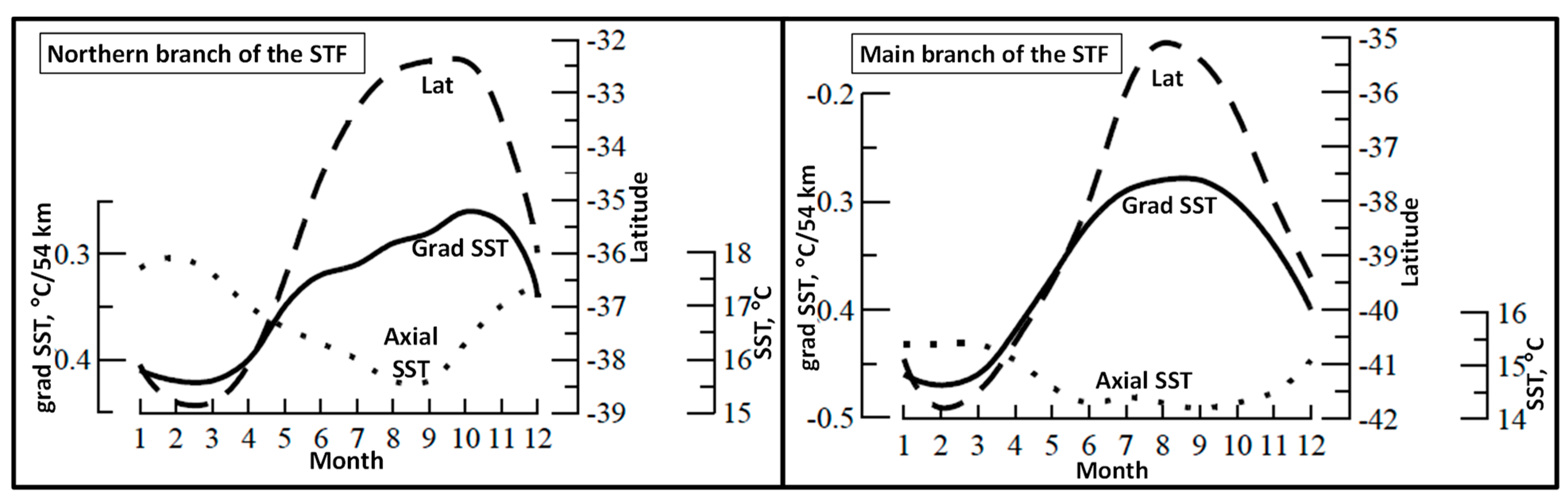
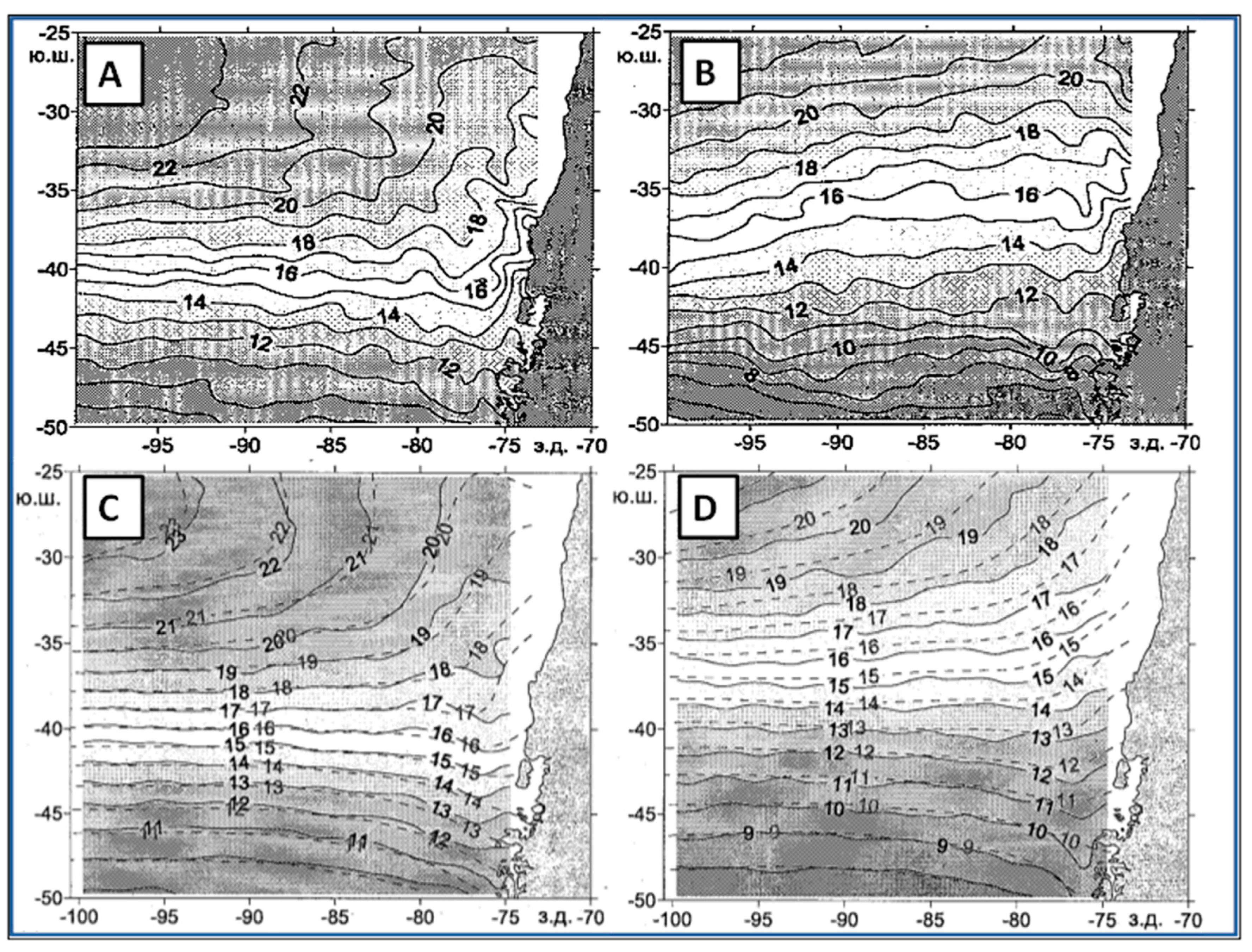
Yu. V. Artamonov and collaborators [21,22,23] identified fronts with local maxima of meridional SST gradient. In a pilot study, Artamonov and Skripaleva [21] detected the STF along 84° W. Instead of a single STF as expected, they found two fronts separated by 3° of latitude. This two-front structure is remarkably consistent with the double-front structure (North and South STF) found by Belkin [3]. Artamonov and Skripaleva [21] reported seasonal variability of both fronts, including their latitude, meridional SST gradient, and axial SST (Figure 3). The axial SST of the NSTF/SSTF varied seasonally between 15.5–18 °C and 14–15.5 °C, respectively.
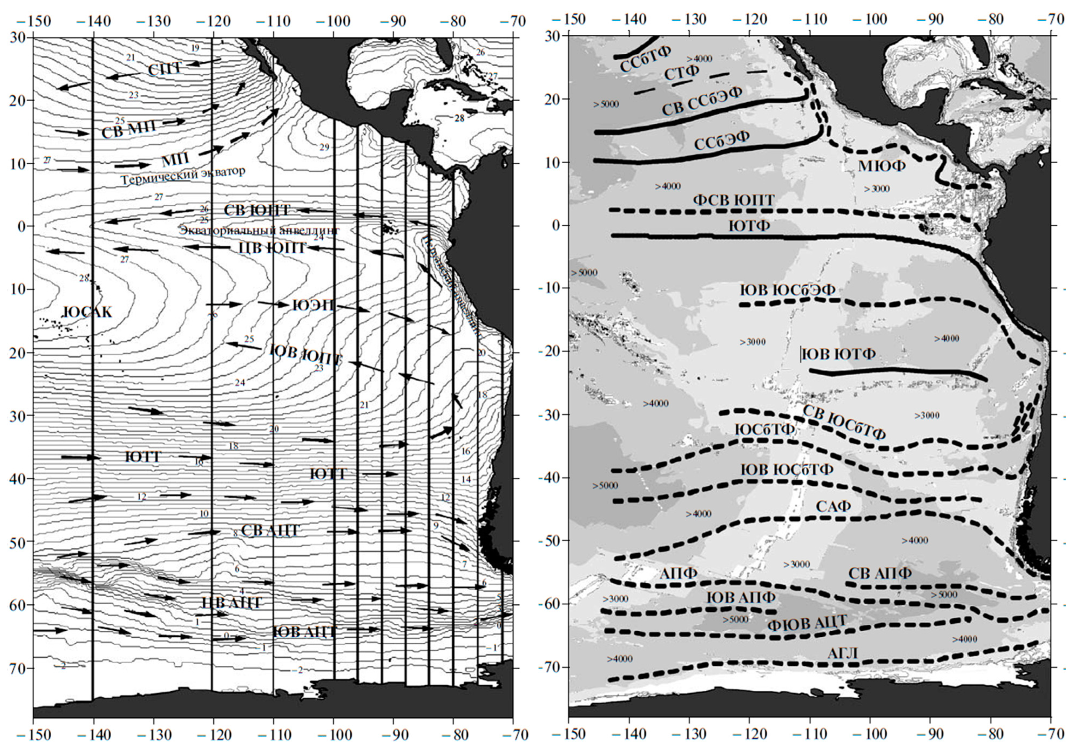
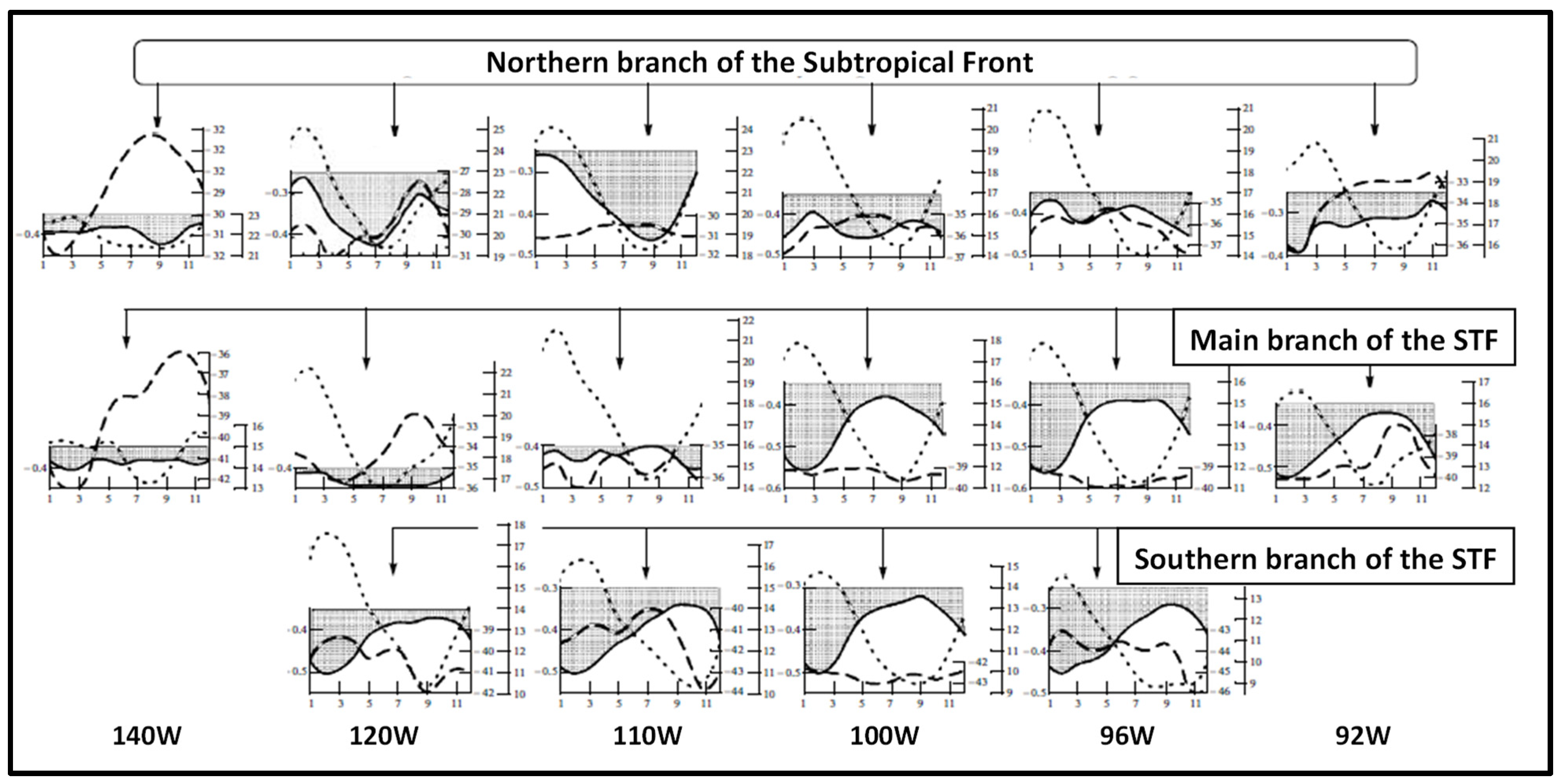
In a follow-up study, Artamonov and Skripaleva [22] mapped SST fronts of the Southeast Pacific east of 145° W (Figure 4 and Figure 5). In addition to the northern branch and main branch of the STF identified by Artamonov and Skripaleva [21] along 84° W, Artamonov and Skripaleva [22] identified the southern branch of the STF.
Artamonov et al. [23] expanded their study across the entire Southern Ocean. In the South Pacific, they mapped SST fronts along 170° E, 170° W, 140° W, 110° W, and 84° W from the Pathfinder AVHRR SST data, 1985–2002. However, this study is less detailed vs. Artamonov and Skripaleva [22], especially in the South Pacific.
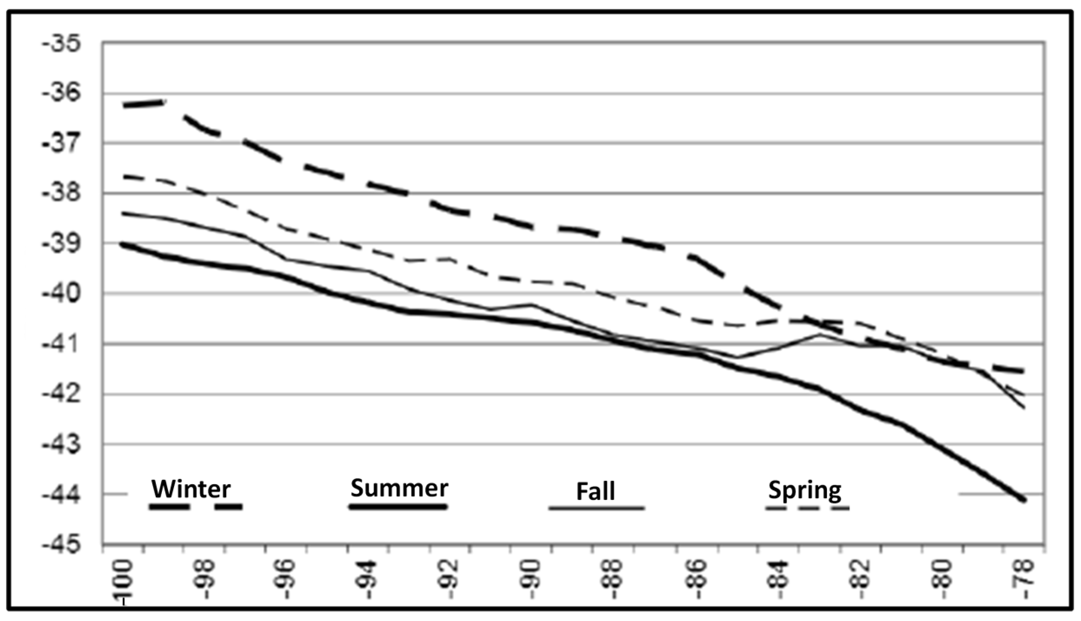
Meanwhile, Gordeeva and Malinin [24] studied the STF’s space-time variability from SST data. They documented the long-term mean path of the STF (Figure 6), revealing a marked non-zonal WNW-ESE spatial trend from 38° S at 100° W down to 42° S at 78° W, contrasting with the near-zonal STF path in Sirota et al. [28] and Lebedev and Sirota [26] (Figure 2).
Gordeeva and Malinin [24] also documented the seasonal variability of the STF. The front migrates from its northernmost location in winter to its southernmost location in summer, with an annual amplitude of seasonal migrations of less than 3° of latitude (Figure 7), which is consistent with similar results by Artamonov and Skripaleva [22]. This consistency throws some doubt onto the six-degree-of-latitude annual amplitude of seasonal migrations along 84° W determined earlier by Artamonov and Skripaleva [21].
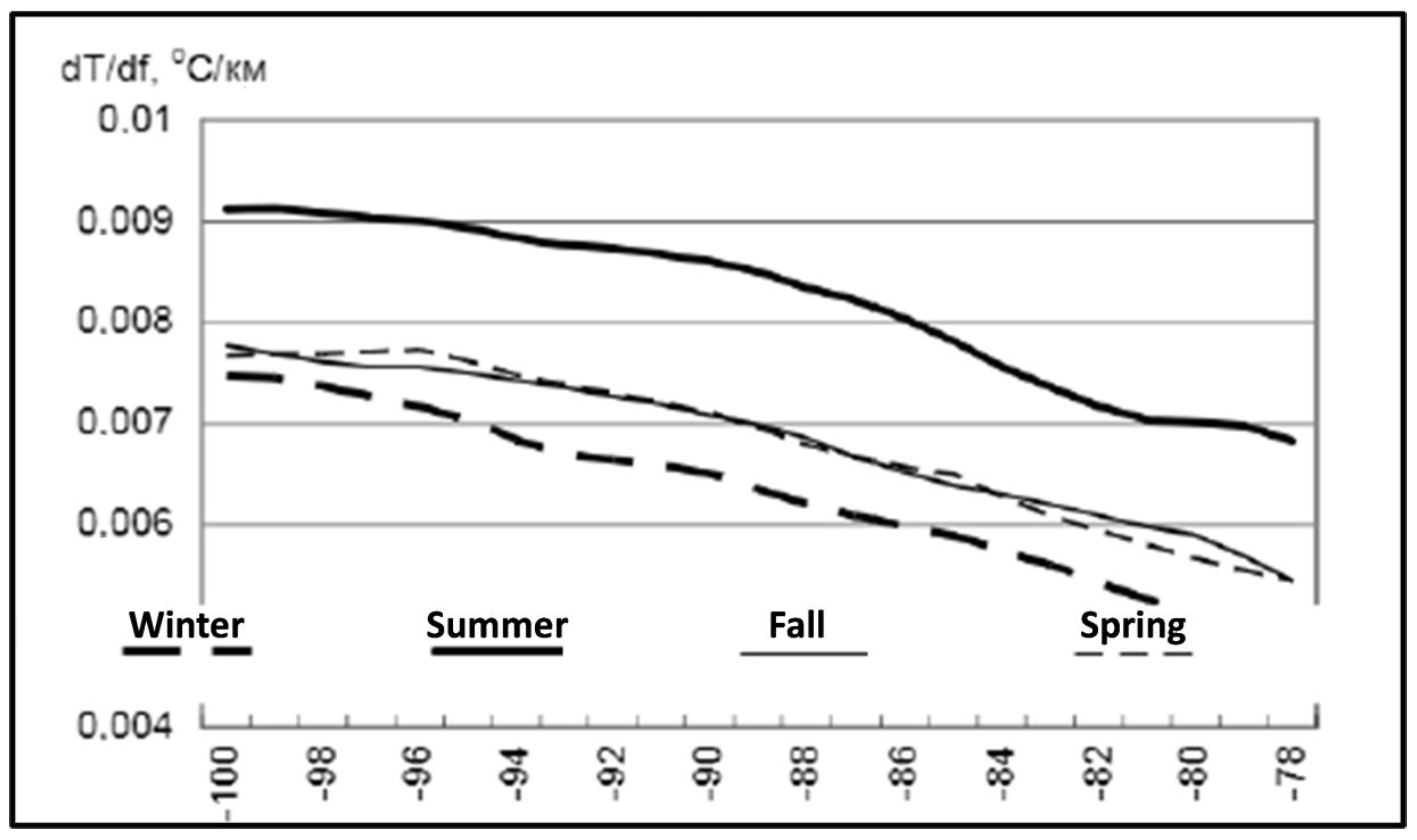
Gordeeva and Malinin [24] also studied seasonal and spatial variability of cross-frontal SST gradient (Figure 8). Across the entire study area (100° W–78° W), the cross-frontal gradient peaks during the austral summer and weakens during the austral winter, which is opposite to the findings by Artamonov and Skripaleva [21] and Artamonov and Skripaleva [22] presented above, especially with regard to the main and southern branch of the STF that feature very weak cross-frontal gradients during the austral summer (February–March).
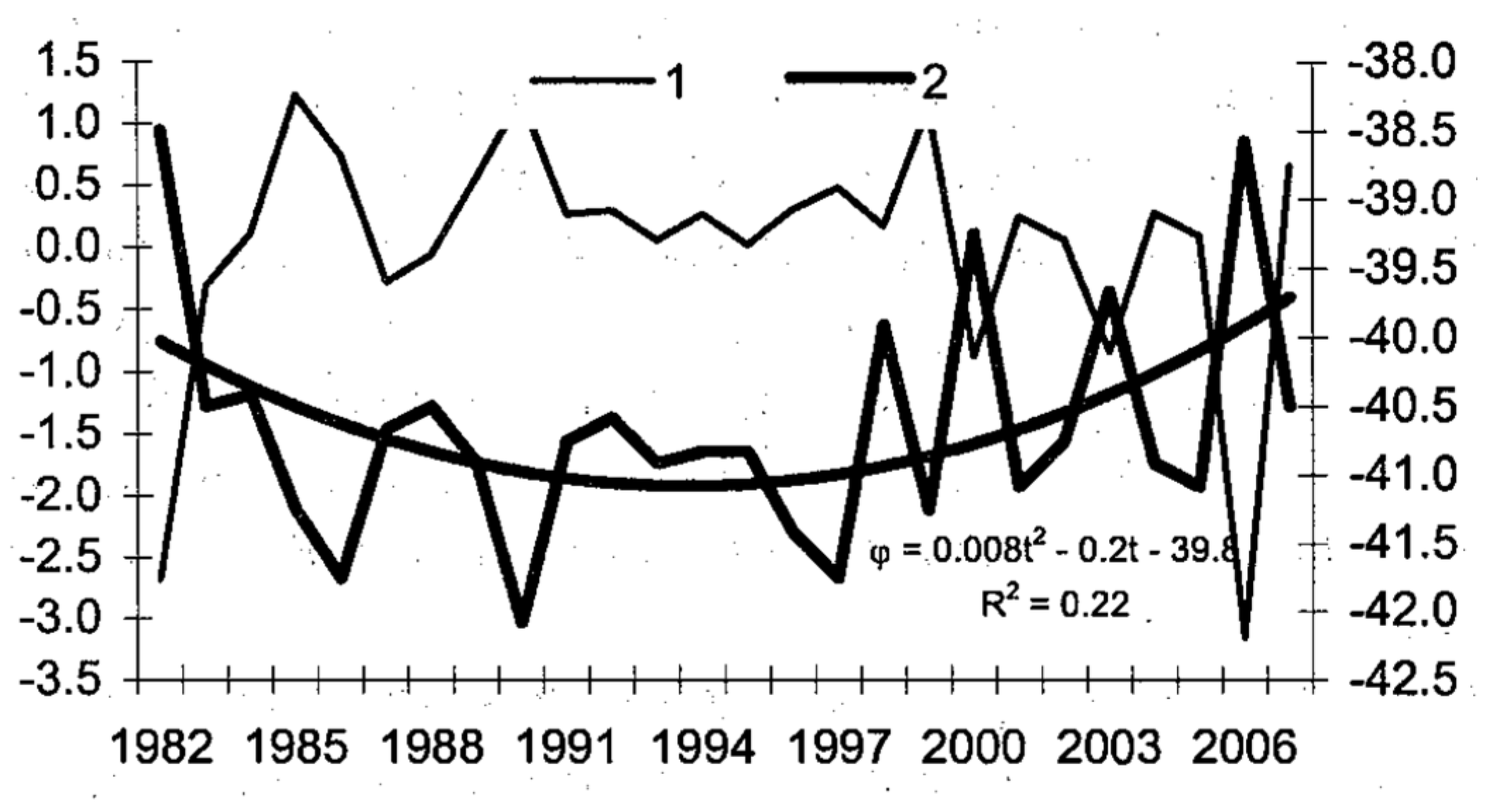
Malinin and Gordeeva [27] documented interannual shifts of the STF along 84.5° W between 1982 and 2006, when the front dipped from 38.5° S to 42° S, then bounced back (Figure 9). This is the only study of the long-term variability of the STF. Therefore, a follow-up study based on a much longer dataset is warranted.
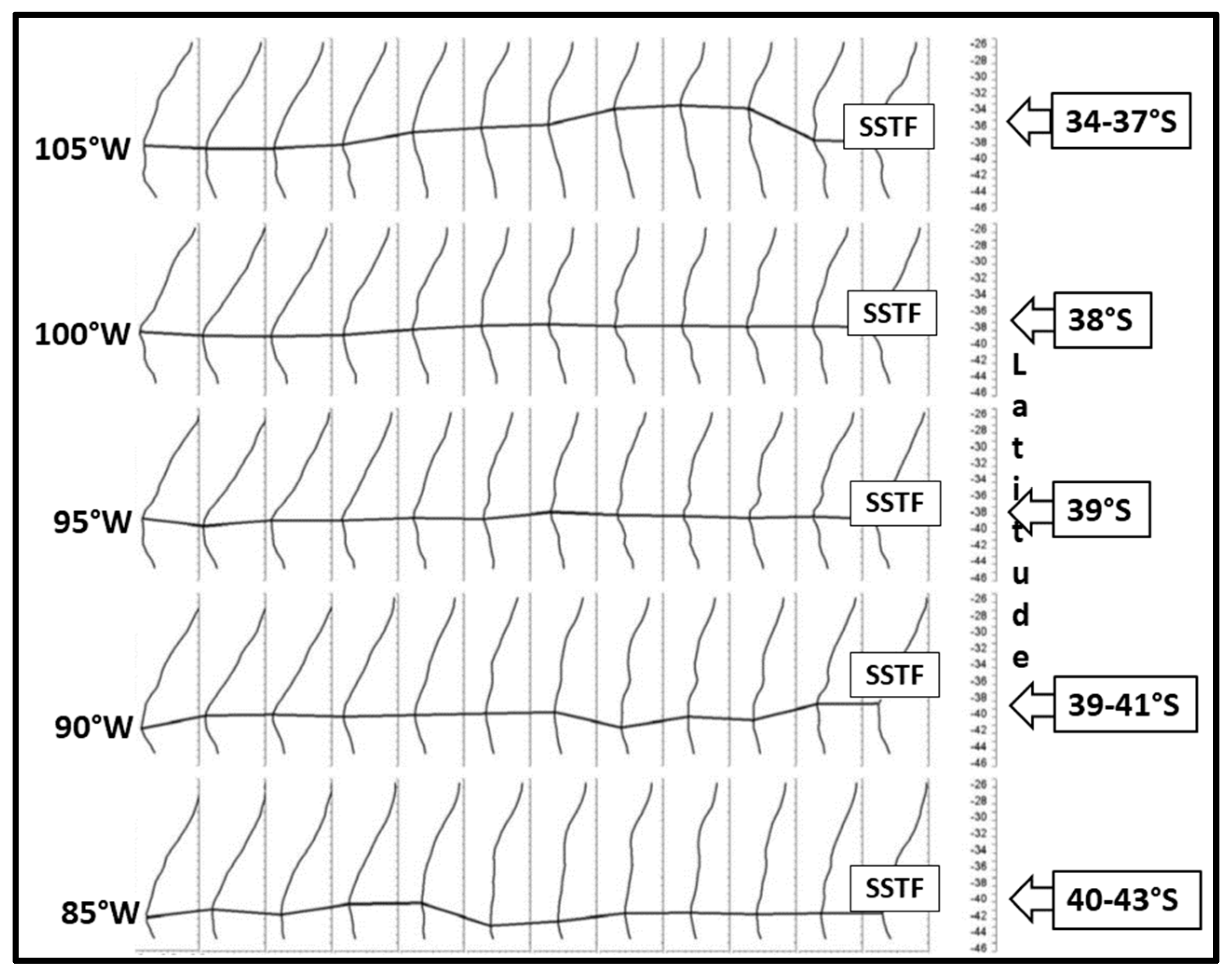
Krasnoborodko [25] studied the STF from SST data in the Southeast Pacific along five meridians between 105° W and 85° W (Figure 10). The most notable result of this study is the strong non-zonal WNW-ESE trend of the STF, from 34° S–37° S at 105° W down to 40° S–43° S at 85° W. Thus, the spatial orientation of the STF in this study agrees quite precisely with the STF climatology by Gordeeva and Malinin [24] presented above.
4. Subtropical Front and the Ecology of Chilean Jack Mackerel Trachurus murphyi
4.1. Jack Mackerel Spawning in the Subtropical Frontal Zone
The key role of the Subtropical Front in the ecology of Chilean jack mackerel (CJM) Trachurus murphyi in the South Pacific was recognized early on. Based on the collections of T. murphyi larvae made off Peru in 1982 and in the central and western South Pacific in 1985, Evseenko [17] pointed out that the spawning area of jack mackerel in the open ocean is confined to the “Subtropical Convergence Zone” (STCZ, the term replaced here by STFZ). The open ocean larvae analyzed by Evseenko [17] were collected during the same cruise (R/V Dmitriy Mendeleyev Cruise 34) when the STFZ was mapped between New Zealand and 126° W [3,12] (Figure 11). Evseenko put the larvae distribution into an oceanographic context by adding to the larvae map the extreme seasonal locations of the 16 °C isotherm in winter (August) and summer (March). Assuming (reasonably) that the larvae caught at 139° W were brought from the west by an eastward current along the STFZ, Evseenko concluded that the spawning area extends westward up to 150–160° W.
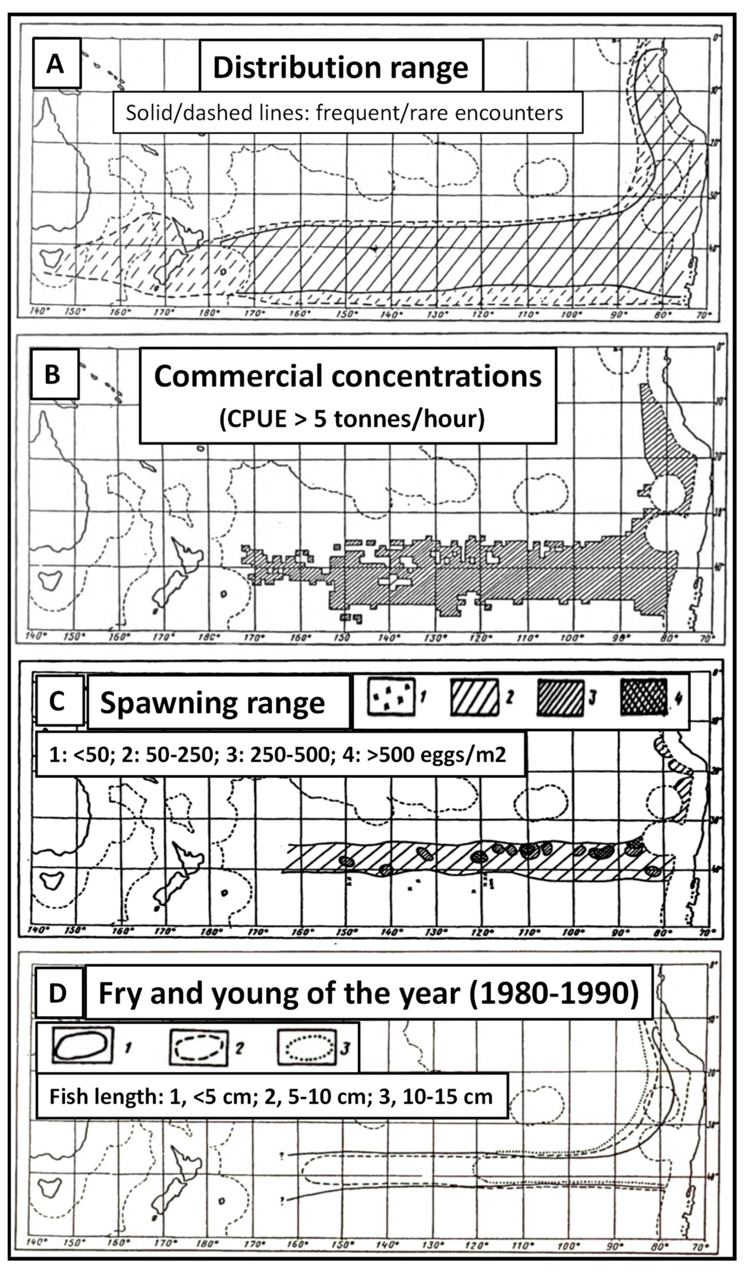
The main conclusion by Evseenko [17] about the CJM spawning within the STCZ was confirmed with a much larger dataset by Bailey [18] who noted (ibid., p. 273): “The predominance of T. murphyi in the diet of albacore suggests that the jack mackerel are abundant between latitudes 34° S and 41° S, longitudes 127° W and 165° W during the austral summer.” Bailey [18] extended the jack mackerel spawning area westward up to the Chatham Rise, presented evidence of the transpacific distribution of jack mackerel along the Subtropical Convergence Zone, and concluded (ibid., p. 277): “It is apparent that Trachurus murphyi is found and likely spawn across the South Pacific from New Zealand to Chile.” The strong spatial correlation between the Subtropical Front (Convergence) and CJM spawning/nursing grounds has been confirmed in numerous studies [31,32,33,34]. Based on data collected in >200 research and fisheries expeditions, Elizarov et al. [35] have documented the CJM range and coined the term “jack mackerel belt” to describe the distribution of T. murphyi in the South Pacific. Elizarov et al. [35] presented two maps showing the entire jack mackerel distribution range that encompasses a wide zonal belt (“distribution belt”) between 34–35° S and 48–50° S (Figure 12A,B) and two maps showing a narrow zonal belt (“spawning belt”) between 34° S and 41° S (Figure 12C,D), the latter coinciding with the STFZ (Figure 1 and Figure 11). The spawning belt is in-between the summer and winter locations of the 16 °C isotherm as postulated by Evseenko ([17], Figure 4). The annual north–south shift of the 16 °C isotherm is about five degrees of latitude (between 35–40° S) as evident from monthly SST maps (Figure 13) (after Malinin and Gordeeva ([27], Figures 5.7 and 5.8). Thus, the annual envelope of the 16 °C isotherm (35–40° S) coincides with both the STFZ (Figure 1 and Figure 11) and CJM spawning belt (Figure 12C,D).
4.2. Population Structure of Jack Mackerel and along-STF Connectivity
Evseenko [17] considered three hypotheses: (1) single population, (2) separate inshore and offshore populations, and (3) offshore population dependent on the inshore population. Evseenko [17] settled at the third hypothesis by eliminating the first two. The population structure of jack mackerel in the South Pacific remained a hotly debated topic ever since as discussed, among others, by Serra [36], Taylor [37], Cárdenas et al. [38], Ashford et al. [39], Gerlotto et al. [40], Vásquez et al. [34], Zhu et al. [41], Dragon et al. [42], Parada et al. [43], and Gerlotto et al. [44].
The eastward South Pacific Current [2] associated with the STF provides physical connectivity (“the along-STF connectivity”) across the South Pacific, where in the open ocean there are no barriers (e.g., submarine ridges) that would help create circulation cells with isolated populations. In the Southwest Pacific, the Louisville Seamount Chain may constrain deep-water and abyssal circulation but not the upper layer (0–300 m) circulation, which is most important to jack mackerel. Only in the easternmost Southeast Pacific, the Juan Fernandez Archipelago serves as a partial barrier to the westerlies and South Pacific Current, creating a low-wind, slow-current area in the wake of the islands, between the archipelago and Chile. This area may serve as an ichthyoplankton retention zone, where Nuñez et al. [33] reported by far the largest concentrations of eggs and larvae of T. murphyi found during November–December.
Drawing upon an extensive review of fisheries and biological data, Serra [36] postulated the existence of two self-sustaining populations, one off Peru and another off Chile, with a boundary between the two stocks “somewhere off southern Peru” (ibid., p. 79). The two-stock concept by Serra [36] has been the organizing focus of many studies, particularly in South America (Julian Ashford, pers. comm., 2021). With regard to the STF, the two-stock concept is of less importance than the “metapopulation” concept (e.g., Gerlotto et al. [40,44]), in which the along-STF connectivity plays a key role. As pointed out by Julian Ashford (pers. comm., 2021), “rather than discrete populations separated by boundaries, the otolith chemistry indicated nucleus chemistry in NZ fish consistent with origin along the STF. The chemistry also suggested that transport in the STF connected life history habitats in the Southeastern Pacific; and heterogeneity was due to extensive mixing between fish from the large spawning zone and smaller, more ephemeral groups surviving in areas with similar conditions along the coast off Chile and Peru”.
4.3. Jack Mackerel Distribution and Subtropical Front
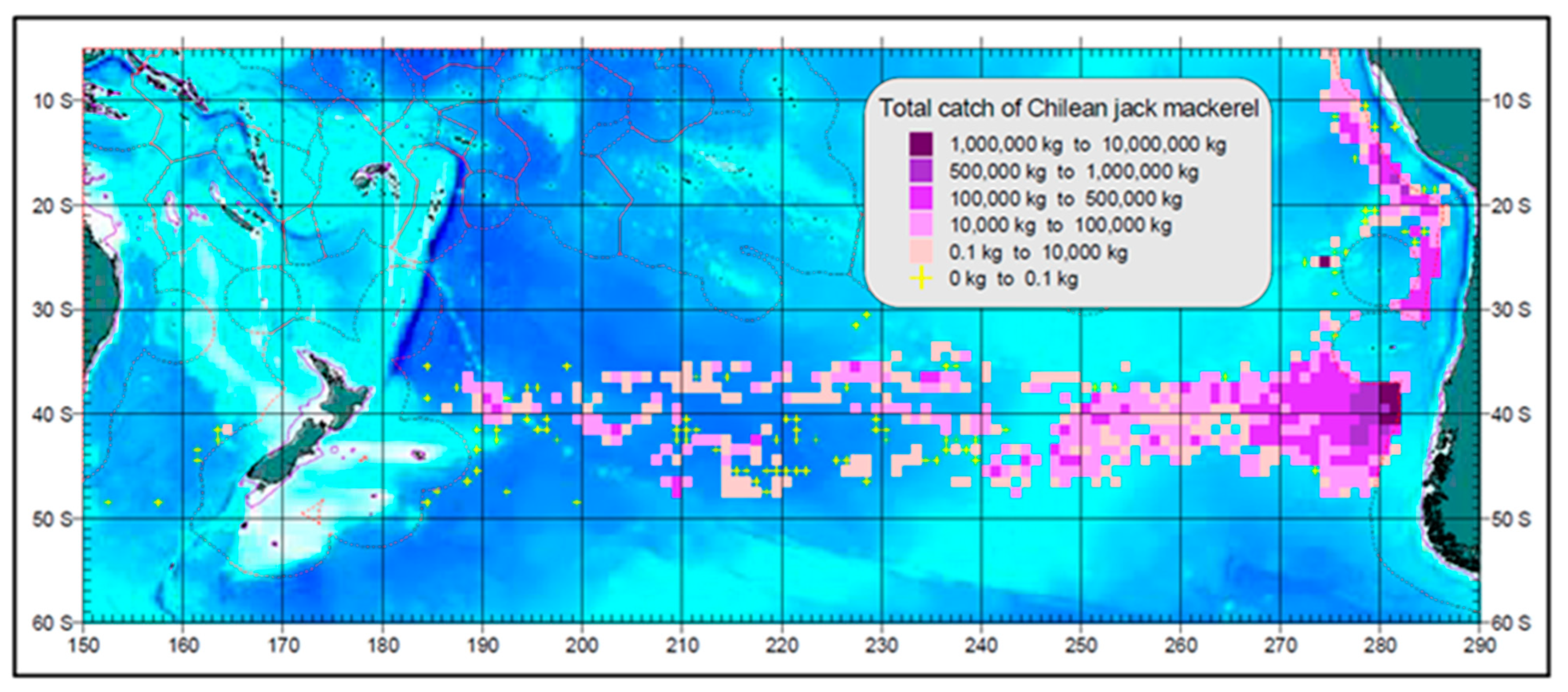
Despite the common recognition of the important role played by the STFZ in the ecology of jack mackerel, very few field studies to date are based on dedicated oceanographic surveys of the STFZ. Instead, most studies resorted to fishery-dependent data from commercial fisheries augmented by remote sensing data such as SST, SSH, and chlorophyll (e.g., Bertrand et al. [45], Li et al. [46], and Parada et al. [43]). The spatial association between the STFZ and T. murphyi is revealed by fishing fleet distribution data. During the maximum extent of Russian fisheries in 1978–1992 (Figure 14) the fleet distribution in the open ocean was spatially congruent with the STFZ, extending zonally across the entire South Pacific from the Chilean EEZ to the New Zealand EEZ in the 34° S–48° S zonal band, aligned with and encompassing the STFZ. The 14-degree latitudinal span of the fleet distribution exceeds the 5-degree latitudinal span of the STFZ (Figure 11) by extending south, down to 48° S, into colder subantarctic waters, where adult fish forage for larger prey as pointed out, among others, by Vinogradov M.E. et al. [47].
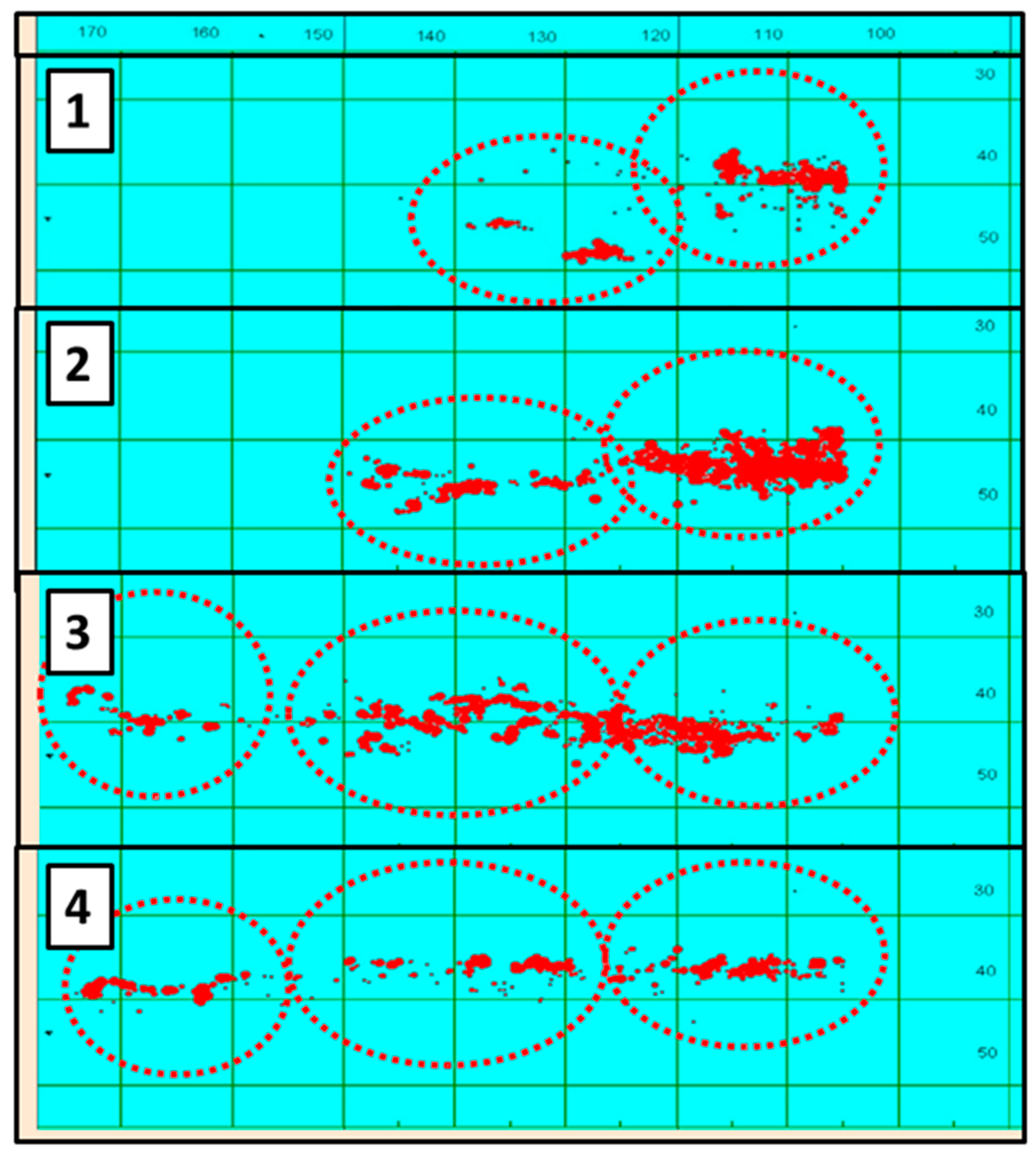
Soldat et al. [50] presented quarterly maps (Figure 15) that imply a rather strong concentration of Russian fishing vessels within a relatively narrow zonal band just a few hundred km wide at a time, extending from Chile westward into the Central South Pacific. This zonal band shifts seasonally, with the annual amplitude of seasonal south-to-north shifts of up to 14° of latitude, from 49° S during the first quarter to 35° S during the fourth quarter, in 1982–1991. Distribution of Chinese fishing vessels [46,51,52] reveals a similar pattern, with the fishing fleet shifting seasonally south-to-north by 10° of latitude, from 47° S in March to 37° S in July, in 2013–2017 ([52], Figure 1). The most detailed annual distribution maps of European fisheries in 2007–2009 ([53], Figures 4–6) reveal steady month-to-month northward progression of the fleet from 47° S in April to 30° S in October, apparently following seasonal migrations of T. murphyi.
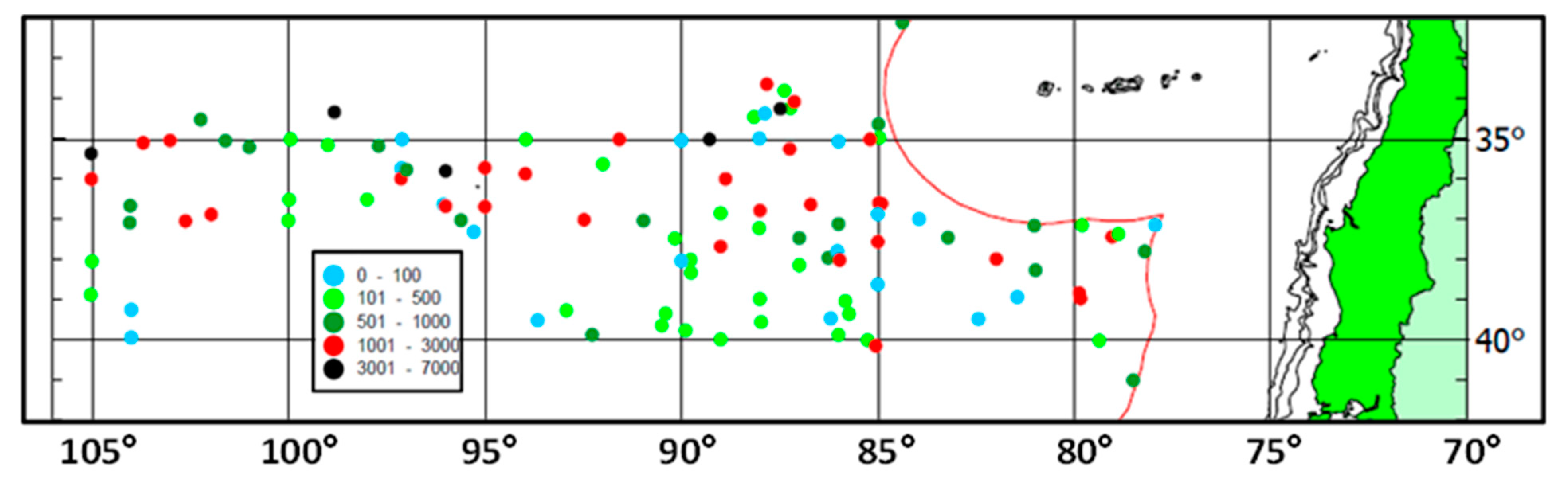
Climatological monthly maps of jack mackerel habitat probability by Bertrand et al. [45] reveal a trans-ocean zonal belt of elevated probabilities in the 35–50° S range (ibid.) aligned with the STFZ envelope (Figure 11). This belt experiences seasonal meridional shifts of about 7–8° of latitude (ibid.). With regards to interannual variability of its location, this zonal belt appears robust (ibid.). The long-term stability of the STFZ location is consistent with Russian fishery distribution data. When, after a 10-year hiatus, the Russian fishery resumed its operations in the Southeast Pacific in 2002, the spatial pattern of the fishery remained intact [54]. The maximum CPUE values were recorded within a narrow zonal belt between 34° S–37° S (Figure 16) nearly collocated with the STFZ (Figure 11). The affinity of T. murphyi to the STFZ seemed to increase westward (Figure 16).
A caveat is warranted regarding possible interpretations of seasonal shifts of fisheries that are often ascribed to the concurrent shifts of the STF. According to this view, the fisheries follow the fish that follow the STF. There are two problems with this interpretation. First, the annual amplitude of seasonal north–south shifts of the STF in the Southeast Pacific is between 1.5° and 3° of latitude, depending on longitude (Figure 7). Meanwhile, as noted above, the annual amplitude of seasonal south-to-north shifts of Russian, Chinese, and European fisheries in the Southeast Pacific is up to, respectively, 14°, 10°, and 17° of latitude. Clearly, there is a gross mismatch between the magnitudes of the seasonal shifts of the fisheries and STF.
The second problem is that the seasonal north-south migrations of jack mackerel are not necessarily caused by the water temperature. Moreover, they are not primarily caused by the water temperature. As pointed out, among others, by Vinogradov M.E. et al. [47], adult fish move south, into colder subantarctic water, in search of larger prey: “The feeding area appears to be between 45 and 50 ° S, where rich feeding grounds are found, providing the most effective foraging. Thus, it should be assumed that seasonal migrations of jack mackerel are determined, not by following the displacement of a hydrological “front”, but by their association with the seasonal change of feeding grounds, different for juveniles and adult fish. Taylor [37] summed up the Vinogradov M.E. et al. [47] conclusions as follows: “Spawning aggregations of jack mackerel occur to the north in waters of the Subtropical Frontal Zone (STFZ) at the frontal break at about 40° S, characterized by small food warm water (summer SST is 16–18 °C), and less seasonal change in plankton biomass than the more southerly zone. Between 45 and 50° S is the feeding zone characterized by rich areas of larger food items. Thus, it follows that seasonal migrations are not due to following the shifts of hydrological fronts, but are associated with seasonal changes in feeding area, which are different for the young and adults.” Without explicitly referring to fronts, Konchina et al. [55] essentially concurred that “the temporal and spatial characteristics of migrations of the Pacific jack mackerel are determined by the temporal and spatial dynamics of species composition and biomass of its main food, meso- and macro-plankton representing the epipelagic and mesopelagic migrating communities”.
4.4. Subtropical Front and Spawning Grounds of Jack Mackerel
The spawning grounds of jack mackerel are associated with a relatively narrow SST range of 15–19 °C typical of the STFZ [32,42]. Based on four ship surveys in oceanic waters (32° S–39° S, 75° W–92° W) off central Chile in November–December 1998–2001, Cubillos et al. ([32], p. 268) concluded that “suitable conditions for spawning could be related to SSTs higher than 15–16 °C. In fact, it is probable that these temperatures are related to the ‘subtropical frontal zone’, to the north of 40° S. In terms of the spawning boundaries, the offshore boundary was never resolved by the surveys, but the main spawning was maximal at 35° S and sea surface temperatures higher than 15–16 °C.” Consistent with other works, numerous Russian studies (including earlier papers reviewed by Taylor [37]) relate the spatial distribution of jack mackerel larvae and juveniles with SST of 15–19 °C typical of the STFZ. Spawning at fronts can be advantageous for fishes owing to the rapid dispersal of fish eggs by current jets associated with most fronts.
4.5. Adult Fishes Leave the Subtropical Frontal Zone to Forage in Subantarctic Waters
Numerous studies focused on temperature ranges preferred by T. murphyi during different life stages, often using SST and certain temperature indices as proxies. There is a consensus regarding T. murphyi spawning at relatively high temperatures typical of the northern periphery of the STFZ. Juveniles remain in or near the STFZ, where they feed mostly on small prey (Figure 12C,D) [35]. Adult fish spend most of their time in colder waters typical of the southern periphery of the STFZ and northern part of the subantarctic zone, south of the STFZ, down to 48° S in the Southeast Pacific, where they feed on larger prey [47]. Since adult fishes forage in northern subantarctic waters south of the STFZ, higher CPUEs are associated with colder SST of 12–15 °C [51]. Seasonal variability of optimum SST ranges associated with highest CPUEs (based on Chinese fishery-dependent data) is documented by Li et al. [46]: Seasonal distributions of SST are approximately Gaussian (except summer), with modal SST of 19 °C, 13 °C, 14 °C, and 15 °C in summer, fall, winter, and spring, respectively. The modal SSTs determined by Li et al. [46] are within the optimum SST ranges determined by Zhang et al. [56]: 15–19 °C in summer, 13–15 °C in fall, 12–14 °C in winter, and 13–16 °C in spring. The main fishing area off central-southern Chile is usually demarcated by the 15 °C isotherm [46,51,57].
4.6. Jack Mackerel’s Affinity to the Subtropical Front
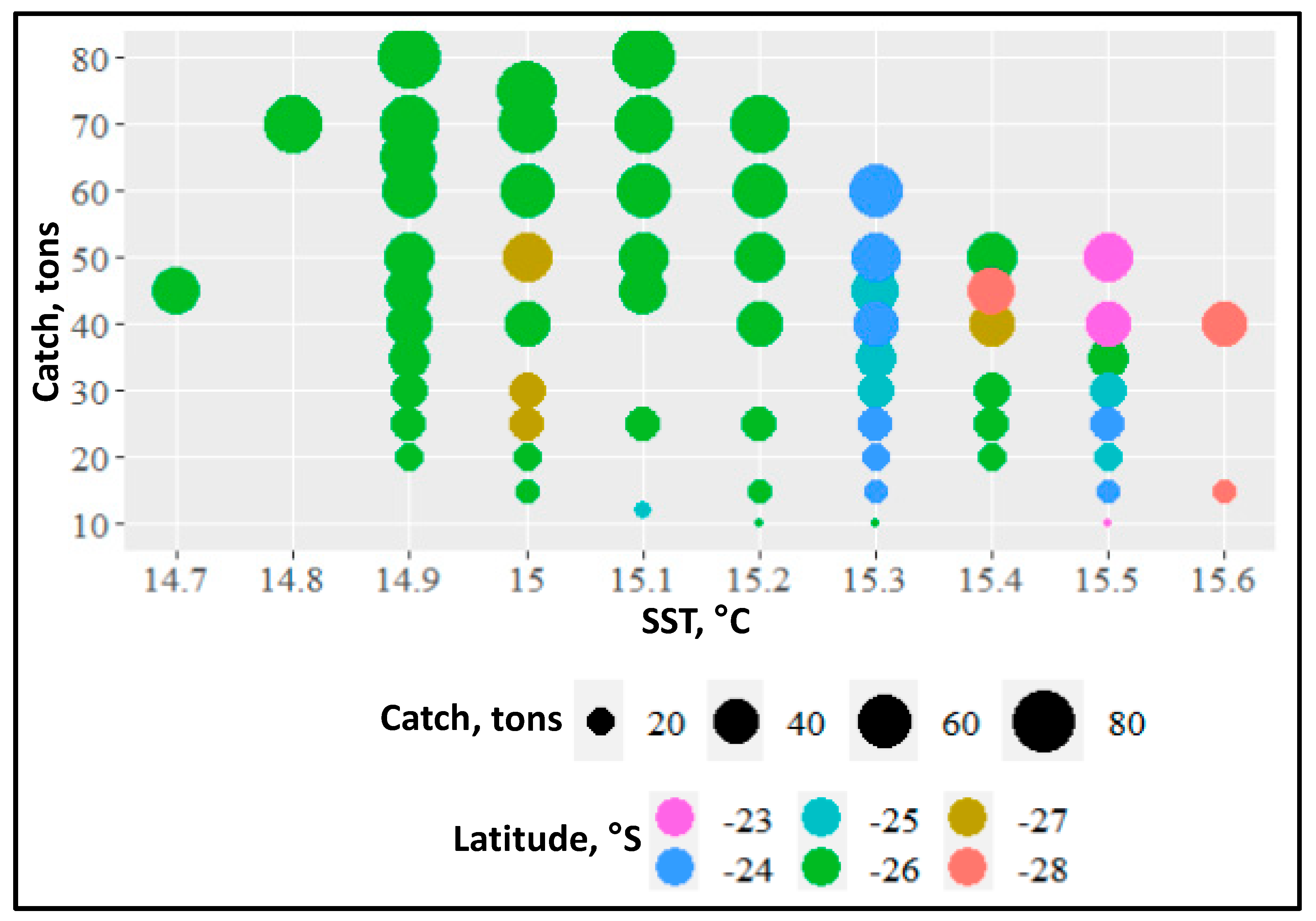
Based on Russian fishery data from austral winter 2020, Dubishchuk [58] reported elevated catches of T. murphyi associated with a narrow range of SST (<1 °C) identified as the STF and spatially confined to just one-degree range of latitudes. Indeed, the maximum catches were linked to SST between 14.9 °C and 15.2 °C observed between 26° S and 27° S (Figure 17). North of 26° S, in warmer waters (SST > 15.5 °C), catches decreased, whereas south of 27° S, in colder waters (SST < 14.7 °C), jack mackerel was nearly absent [58]. The extremely narrow range of SST associated with maximum CPUE is suggestive of jack mackerel seeking the water mass convergence embedded into the front and probably using water temperature and salinity as cues. Such front-related convergences feature elevated concentrations of zooplankton, the main prey of jack mackerel.
4.7. Migration of Jack Mackerel along the Subtropical Front
The jack mackerel’s length and age in the South Pacific increases westward (e.g., [59]). The most obvious explanation of this trend is the westward migration of jack mackerel. The eastward South Pacific Current (approximately collocated with the STFZ) is rather sluggish, with mean surface velocities of 2 cm/s east of 100° W [8] and geostrophic transport of 2 to 5 Sv [2]. Therefore, the jack mackerel could swim long distances against this current without expending too much energy fighting the opposing current. Konchina et al. [55] reported: “Our analysis proves that before reaching sexual maturity (at the age of three years), the young jack mackerel (20–26 cm, two-year-olds) successfully forage and grow in oceanic epipelagic waters. The ranges of feeding migrations of the mackerel juveniles [may be] extensive because fish at the length of 20 cm (1 yr) can move 280–840 nautical miles in a month.” Konchina and Pavlov [60] emphasized the importance of strong year classes. Such dominant cohorts tend to migrate west along the STFZ toward New Zealand as visualized by Grechina [61] and Gerlotto et al. [40], albeit without explicitly referring to the STFZ as the migration corridor. Horn and Maolagáin [59] analyzed otoliths from T. murphyi collected off New Zealand in 2007–2019 and concluded that there were at least two invasions of jack mackerel from the high seas into the New Zealand waters. The STFZ is the most plausible path taken by the immigrant T. murphyi coming toward New Zealand from the east.
There are two mechanisms facilitating the westward migration of jack mackerel in the South Pacific: (1) westward countercurrent proposed by McGinnis [62]; (2) westward propagation of mesoscale eddies documented by Chaigneau and Pizarro [7]. McGinnis [62] mapped spatial distribution of lanternfish larvae that revealed a distinct trend of westward increase of larval age. Since the larvae are poor swimmers, they are passive tracers of ocean currents. Thus, McGinnis [62] concluded that the larvae are carried to the west by a westward current that flows against the broad eastward West Wind Drift. Deacon [63] supported McGinnis’ hypothesis by pointing out the existence of a westward wedge of low-salinity water in the subantarctic zone west of Chile as a proof of a westward current. The low-salinity wedge originates off the Chilean coast owing to the copious amount of precipitation falling onto the western slopes of the Andes and feeding numerous rivers draining the slopes [64,65]. For an alternative, model-based explanation of the westward wedge of low salinity, see Karstensen [66].
The existence of a westward current was further supported by Neshyba and Fonseca [67] and Uribe et al. [68] who conducted an oceanographic survey based on a meridional high-resolution (11 km) XBT section along 92° W, from 45° to 35° S, in February 1979, and presented physical evidence of a counterflow to the eastward West Wind Drift corroborated by biological evidence based on the biogeography of phytoplankton sampled during the oceanographic survey, particularly the pennate diatom Nitzshcia longissimi, which is “generally associated with shallow coastal waters and which comprises a major fraction of the phytoplankton assemblage near the frontal zone [STFZ] but within the low-salinity tongue.” ([68], p. 1229).
Another mechanism that explains the observed length/age distribution of Chilean jack mackerel in the South Pacific is the westward movement of mesoscale eddies (“eddy trains”) generated off Chile documented by Chaigneau and Pizarro [7] and Belmadani et al. [69,70]. For any marine animal (including fish) inside a mesoscale eddy in this region, traveling westward with the eddy is energetically advantageous vs. swimming against the eastward currents that dominate this region. In addition to the “free ride” inside westward-moving mesoscale eddies, fish may seek out such eddies owing to the prey concentration inside mesoscale eddies. The affinity of various marine animals, including fish, to mesoscale eddies has been documented in numerous studies, some of them reviewed by Belkin [71].
The continuous migration along the STFZ is consistent with the concept of a single population (or pelagic meta-population) of jack mackerel encompassing the entire subtropical–subantarctic belt between Chile and New Zealand [38,45]. An alternative concept envisions a few distinct populations (or sub-populations) of T. murphyi within the STFZ [35,39,40,42,43,50]. From a purely oceanographic viewpoint, the multi-stock hypothesis lacks strong support. Indeed, the relatively smooth bathymetry inside this latitudinal belt could not play any substantial role in the presumed isolation of such individual stocks from one another. There are no meridional topographic barriers (steep submarine ridges or seamount chains like the Louisville Seamount Chain in the Southwest Pacific) that could facilitate the emergence of circulation cells in the upper few hundred meters that could serve as habitats of choice for isolated populations of T. murphyi.
Nonetheless, seamounts in the 33–39° S, 105–120° W area could play a certain role in the formation of a partly isolated spawning/nursery ground as argued by Parada et al. [43], especially because this area is traversed by the STFZ [3,9,13,14] and associated South Pacific Current [2,8]. These seamounts can impede the westward propagation of mesoscale eddies emanated from the Chile–Peru Current [7], thereby contributing to the formation of a shadow zone of eddy activity [43] favorable for the existence of an isolated population of T. murphyi.
5. Discussion
5.1. Spatial Discordance between Temperature and Salinity Manifestations of the STF
All remote sensing studies based on SST data and reviewed in Section 3 arrived at the same spatial trend: Namely, in the Southeast Pacific, the SST-based STF/STFZ extends from WNW to ESE. At the same time, studies based on in-situ hydrographic data [2,72] arrived at a different spatial trend: Across the entire South Pacific, the salinity-based STF/STFZ extends from WSW to ENE. The dynamic STF (identified with maximum gradient of SSH) is approximately zonal across the Southeast Pacific (see Section 3), thus being spatially dissociated from either the temperature or salinity manifestations of the STF. The spatial discordance between thermohaline and dynamic manifestations of the STF in the Southern Ocean was previously reported by Stramma and Peterson [73], Stramma [74], Stramma and Lutjeharms [75], James et al. [76], Tippins and Tomczak [30], Wong and Johnson [77], Hamilton [78], and Graham and de Boer [29], and was attributed to the density compensation of temperature and salinity across the STF. This phenomenon was also observed by Rudnick and Ferrari [79] in the North Pacific, where thermohaline fronts in the upper mixed layer on horizontal scales from 20 m to 10 km were found to be density-compensated.
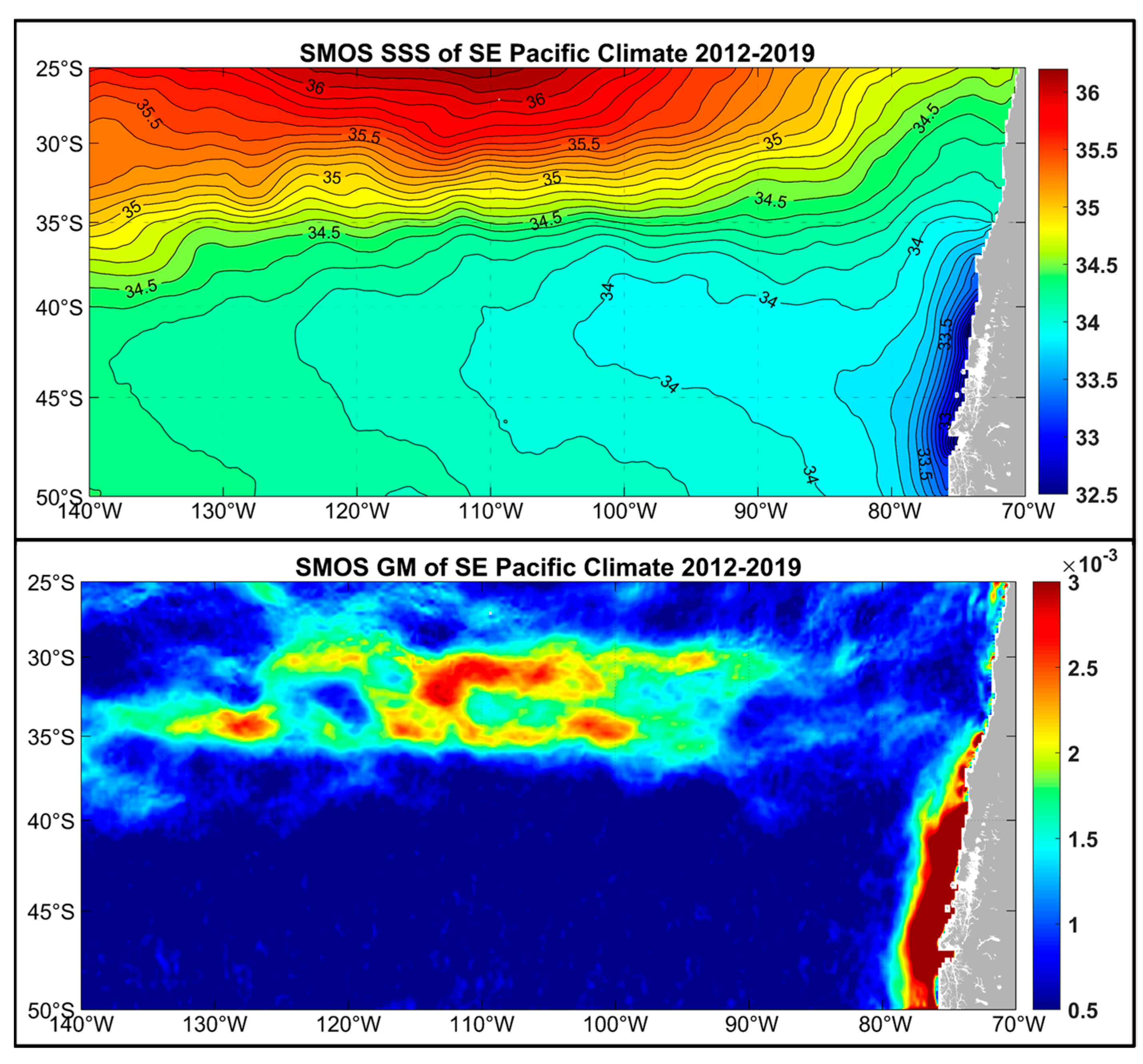
Recently, the authors explored the potential of satellite SSS data application for front mapping in the Southern Ocean, particularly with regard to the STF mapping. Using SMOS data from 2012–2019, we studied seasonal and interannual variability of the SSS manifestation of the circumpolar STFZ. Here we present two maps (SSS and grad SSS) from the Southeast Pacific (Figure 18). The grad SSS map shows the STFZ as a broad (5° of latitude) zonal frontal zone between 30° S and 35° S. Monthly maps of grad SSS (not shown) reveal an intricate internal structure of the STFZ consisting of multiple disconnected frontal segments. These maps also show relatively small (1–2° of latitude) seasonal north-south shifts of the SSS-defined STFZ.
5.2. Salinity Data in Fish Ecology
Very few population models to date used salinity and salinity gradient as explanatory variables, even though the STF is well known as a distinct salinity front [2,3,72]. The Chilean jack mackerel was reported to prefer a very narrow range of salinities (34.9–35.1 [19]). These salinities are typical of the STF [3], which is suggestive of the fish using salinity as a cue to locate the STF. Owing to the important ecological role of the STF, salinity and salinity gradients should be included into population models. This is not always the case, even in recent studies (e.g., [80]). Using habitat suitability index (HSI) models to examine spatial patterns of Dosidicus gigas (Humboldt squid) and Trachurus murphyi off Chile, Feng et al. [81] used SSS for D. gigas but not for T. murphyi even though SSS data for the latter was available. In most case studies, the dearth of salinity data remains a major impediment to the inclusion of salinity into various models. Even when XBT data are collected every 30 to 40 km along shipping lanes crossing the STFZ, salinity data are collected less frequently by expensive XCTDs [77]. The data paucity problem could be solved by the development of automated flow-through thermosalinographs (TSG) for fishing fleets operating in the STFZ. The full potential of satellite SSS data should be utilized as well. Our ongoing study has shown that satellite SSS data can be used to map large-scale fronts in the Southern Ocean (Figure 18).
5.3. Fronts (Gradients) in Population Models
The existing population models of jack mackerel include temperature among other explanatory environmental variables. None of the existing population models of jack mackerel includes fronts or gradients as proxies of fronts. At the same time, anecdotal evidence mounts of fishers actively seeking out fronts as habitats of choice for jack mackerel, at least during certain life stages. For example, during the R/V Dmitry Mendeleyev Cruise 34 in 1985, surface temperature and salinity fronts in the Central South Pacific were documented continuously underway in real time using a flow-through thermosalinograph connected to the ship’s water intake [3,10,11]. The coordinates and TS-ranges of the fronts crossed by R/V Dmitry Mendeleyev were radioed daily to the nearby MV Pioner Nikolaeva (large freezer-trawler), where Dr. Nikolai Shurunov used the front data to target jack mackerel and improve the efficiency of the ship’s fishing operations.
5.4. Front Data in Marine Ecology and Fisheries
A strong case can be made for using front data in marine ecology and fisheries. The systematic use of satellite data from various missions and state-of-the-art front detection algorithms (reviewed recently by Belkin [71]) would likely have a synergetic effect. Technically and logistically, all components are available for an efficient implementation of a front-centric computerized system for jack mackerel fisheries. For instance, Gordeeva and Zharova [82] used SST and SSH data to provide STF forecasts in assistance to the Chilean jack mackerel fisheries in the Southeast Pacific. The most difficult aspect of a forecast system is the need to account for qualitatively different strategies used by jack mackerel during different life stages. For example, a strong link between jack mackerel and STF during spawning does not exist later during nursing and foraging stages, when adult fish leave the STF and move south for colder subantarctic waters with larger prey items. This is a generic species-specific problem of marine animals moving across the ocean realm between different life stages, sometimes migrating from one large-scale front to another as pointed out, among others, by Belkin et al. [83].
6. Data Gaps, Knowledge Gaps, and Key Next Steps
Major data gaps hinder applications of remote sensing in marine fisheries and population management of various fishes, including Chilean jack mackerel, in the Southeast Pacific. In particular, comprehensive up-to-date climatology of the Subtropical Front in the open South Pacific is missing. Such a climatology should combine in-situ data (however patchy and sparse) and satellite data. The existing studies reviewed in this work have been largely based on satellite SST data. Salinity data, including satellite SSS, were all but ignored until recently. No attempts were made until 2021 to consider the Subtropical Front in the South Pacific as an integral part of the circumpolar Subtropical Frontal Zone [84]. Even though SST maps are routinely used by international deep-sea fisheries, particularly by Russian and Ukrainian fleets in the open Southeast Pacific, no systematic studies of SST fronts in this region have been published after 2009 save for a single paper in 2017 (see Section 3 above). All studies reviewed in this work were based on old SST data (through 2006). This means, inter alia, that possible regional manifestations of the ongoing global warming that took place in this region since 2006 remain undocumented and unaccounted for. These studies used long-term mean monthly data that are not suitable for front detection owing to the inevitable smoothing during averaging and also due to the relatively low spatial resolution of long-term mean data sets (Table 1).
Key next steps that can be envisioned at this point will be three-pronged [71]. First, various satellite missions provide SST, SSS, and SSH data that should be utilized in near-real time and delayed mode. Second, fronts (gradients of physical, chemical, and biological properties) should be integrated into population models. Third, advanced algorithms for front detection are available that should be used for front mapping in fisheries research, operational support of deep-sea fisheries, and population modeling.
7. Conclusions
In the South Pacific, the Subtropical Front consists of two fronts, North and South STF, that bound the Subtropical Frontal Zone (STFZ) in-between. The STF plays a key role in the ecology of Chilean jack mackerel Trachurus murphyi that spawn at the STF and migrate along the STF from Chile up to New Zealand. The STF is density-compensated, with spatially divergent manifestations in temperature and salinity. Several studies of the STF from satellite SST data reveal a robust spatial trend from WNW to ESE in the Southeast Pacific. In the salinity field, the STF’s orientation is different as the haline STF extends from WSW to ENE across the entire South Pacific. Various data on T. murphyi distribution in the South Pacific (including spatial data on spawning and catch statistics) are consistent with T. murphyi spawning, nursing, foraging, and migrating within the STFZ; adult fishes forage mostly in colder subantarctic waters south of the STFZ. Three major types of remote sensing data-SST, SSH, and SSS-can be used to locate the STFZ. The SSH data is most advantageous to the jack mackerel fisheries owing to the all-weather capability of satellite altimetry and the radical improvement of the spatial resolution of SSH data in the near future.
Author Contributions
I.M.B.: Conceptualization, methodology, and writing; X.-T.S.: data curation, analysis, and visualization. All authors have read and agreed to the published version of the manuscript.
Funding
This research received no external funding.
Data Availability Statement
No new data have been created for this study. Data sharing is not applicable to this article.
Acknowledgments
Julian Ashford and three anonymous reviewers made important suggestions that helped improve this manuscript. Daphne Johnson created the circumpolar frontal map in Figure 1 with the ODV software. David Peterman provided a PDF of Elizarov et al. (1993), from which four maps were reproduced (with modifications). Igor Belkin is most grateful to his colleagues, participants in the R/V Dmitriy Mendeleyev Cruise 34 (Mikhail Vinogradov, Chief Scientist), during which the Subtropical Frontal Zone in the South Pacific was discovered. While working on this paper, Igor Belkin and Xin-Tang Shen were supported by the College of Marine Science and Technology, Zhejiang Ocean University, Zhoushan, China.
Conflicts of Interest
The authors declare no conflict of interest.
References
- Lima, M.; Canales, T.M.; Wiff, R.; Montero, J. The interaction between stock dynamics, fishing and climate caused the collapse of the jack mackerel stock at Humboldt Current ecosystem. Front. Mar. Sci. 2020, 7, 123. [Google Scholar] [CrossRef]
- Stramma, L.; Peterson, R.G.; Tomczak, M. The South Pacific Current. J. Phys. Oceanogr. 1995, 25, 77–91. [Google Scholar] [CrossRef]
- Belkin, I.M. Main hydrological features of the Central South Pacific. In Ecosystems of the Subantarctic Zone of the Pacific Ocean; Vinogradov, M.E., Flint, M.V., Eds.; Nauka: Moscow, Russia, 1988; pp. 21–28, English translation: Pacific Subantarctic Ecosystems; New Zealand Translation Centre Ltd.: Wellington, New Zealand, 1997; pp. 12–17. [Google Scholar]
- Belkin, I.M. Frontal structure of the South Atlantic. In Pelagic Ecosystems of the Southern Ocean; Voronina, N.M., Ed.; Nauka: Moscow, Russia, 1993; pp. 40–53. (In Russian) [Google Scholar]
- Belkin, I.M.; Gordon, A.L. Southern Ocean fronts from the Greenwich meridian to Tasmania. J. Geophys. Res. Ocean. 1996, 101, 3675–3696. [Google Scholar] [CrossRef]
- Schlitzer, R. Ocean Data View. 2022. Available online: https://odv.awi.de (accessed on 4 December 2022).
- Chaigneau, A.; Pizarro, O. Eddy characteristics in the eastern South Pacific. J. Geophys. Res. Ocean. 2005, 110, C06005. [Google Scholar] [CrossRef]
- Chaigneau, A.; Pizarro, O. Mean surface circulation and mesoscale turbulent flow characteristics in the eastern South Pacific from satellite tracked drifters. J. Geophys. Res. Ocean. 2005, 110, C05014. [Google Scholar] [CrossRef]
- Chaigneau, A.; Pizarro, O. Surface circulation and fronts of the South Pacific Ocean, east of 120° W. Geophys. Res. Lett. 2005, 32, L08605. [Google Scholar] [CrossRef]
- Belkin, I.M.; Gritsenko, A.M.; Kryukov, V.V. Thermohaline structure and hydrological fronts. In Ecosystems of the Subantarctic Zone of the Pacific Ocean; Vinogradov, M.E., Flint, M.V., Eds.; Nauka: Moscow, Russia, 1988; pp. 28–36. (In Russian); English translation: Pacific Subantarctic Ecosystems; New Zealand Translation Centre Ltd.: Wellington, New Zealand, 1997; pp. 18–23 [Google Scholar]
- Belkin, I.M.; Gusev, Y.M.; Levin, L.A. Surface thermohaline fronts of the South Pacific. In Ecosystems of the Subantarctic Zone of the Pacific Ocean; Vinogradov, M.E., Flint, M.V., Eds.; Nauka: Moscow, Russia, 1988; pp. 36–47. (In Russian); English translation: Pacific Subantarctic Ecosystems; New Zealand Translation Centre Ltd.: Wellington, New Zealand; 1997; pp. 24–29 [Google Scholar]
- Vinogradov, M.E.; Flint, M.V. (Eds.) Ecosystems of the Subantarctic Zone of the Pacific Ocean; Nauka: Moscow, Russia; p. 304. (In Russian); English translation: Pacific Subantarctic Ecosystems; New Zealand Translation Centre Ltd.: Wellington, New Zealand, 1997, p. 243.
- Tsuchiya, M.; Talley, L.D. Water-property distributions along an eastern Pacific hydrographic section at 135W. J. Mar. Res. 1996, 54, 541–564. [Google Scholar] [CrossRef]
- Tsuchiya, M.; Talley, L.D. A Pacific hydrographic section at 88° W: Water-property distribution. J. Geophys. Res. Ocean. 1998, 103, 12899–12918. [Google Scholar] [CrossRef]
- González Carman, V.; Piola, A.; O’Brien, T.D.; Tormosov, D.D.; Acha, E.M. Circumpolar frontal systems as potential feeding grounds of Southern Right whales. Prog. Oceanogr. 2019, 176, 102123. [Google Scholar] [CrossRef]
- Clay, T.A.; Phillips, R.A.; Manica, A.; Jackson, H.A.; de Brooke, M.L. Escaping the oligotrophic gyre? The year-round movements, foraging behaviour and habitat preferences of Murphy’s petrels. Mar. Ecol. Prog. Ser. 2017, 579, 139–155. [Google Scholar]
- Evseenko, S.A. On the reproduction of the Peruvian jack mackerel, Trachurus symmetricus murphyi (Nichols), in the Southern Pacific. J. Ichthyol. 1987, 27, 151–160. [Google Scholar]
- Bailey, K. Description and surface distribution of juvenile Peruvian jack mackerel, Trachurus murphyi, Nichols from the subtropical convergence zone of the central South Pacific. Fish. Bull. 1989, 87, 273–278. [Google Scholar]
- Gerlotto, F.; Dioses, T. Bibliographical Synopsis on the Main Traits of life of Trachurus murphyi in the South Pacific Ocean. SPRFMO 2013, SC-01-INF-17. In Proceedings of the 1st Meeting of the Scientific Committee, La Jolla, CA, USA, 21–27 October 2013; p. 217. [Google Scholar]
- Haddaway, N.R.; Macura, B.; Whaley, P.; Pullin, A.S. ROSES RepOrting standards for Systematic Evidence Syntheses: Pro forma, flow-diagram and descriptive summary of the plan and conduct of environmental systematic reviews and systematic maps. Environ. Evid. 2018, 1998, 7. [Google Scholar] [CrossRef]
- Artamonov, Y.V.; Skripaleva, E.A. Variability of hydrological fronts in the Peru-Chilean sector from satellite data. Ukr. Antarct. J. 2006, 5, 109–116. (In Russian) [Google Scholar] [CrossRef]
- Artamonov, Y.V.; Skripaleva, E.A. Seasonal variability of the large-scale fronts in the Eastern Pacific based on satellite data. Earth Stud. Space 2008, 4, 45–61. (In Russian) [Google Scholar]
- Artamonov, Y.V.; Skripaleva, E.A.; Babiy, M.V.; Galkovskaya, L.K. Seasonal and interannual variability of the hydrological fronts in the Southern Ocean. Ukr. Antarct. J. 2009, 8, 205–216. (In Russian) [Google Scholar] [CrossRef]
- Gordeeva, V.N.; Malinin, V.N. Large-scale variability of the South Subtropical Front in the south-eastern part of the Pacific Ocean. Vestn. Immanuel Kant Balt. Fed. Univ. 2006, 2, 160–169. (In Russian) [Google Scholar]
- Krasnoborodko, O.Y. Formation of local frontal zones and mesoscale dynamics of waters in the southern part of Pacific Ocean. Tr. VNIRO 2017, 169, 136–141. (In Russian) [Google Scholar]
- Lebedev, S.A.; Sirota, A.M. Oceanographic investigation in the Southeastern Pacific Ocean by satellite radiometry and altimetry data. Adv. Space Res. 2007, 39, 203–208. [Google Scholar] [CrossRef]
- Malinin, V.N.; Gordeeva, S.M. Fisheries Oceanography of the Southeast Pacific: Variability of Habitat Factors; St. Petersburg State University Publishing House: St. Petersburg, Russia, 2009; Volume 1, p. 278. (In Russian) [Google Scholar]
- Sirota, A.M.; Lebedev, S.A.; Timokhin, E.N.; Chernyshkov, P.P. Application of Satellite Altimetry for Diagnostics of Fisheries Oceanography Conditions in the Atlantic Ocean and Southeast Pacific; AtlantNIRO: Kaliningrad, Russia, 2004; p. 68. (In Russian) [Google Scholar]
- Graham, R.M.; De Boer, A.M. The Dynamical Subtropical Front. J. Geophys. Res. Ocean. 2013, 118, 5676–5685. [Google Scholar] [CrossRef] [Green Version]
- Tippins, D.; Tomczak, M. Meridional Turner angles and density compensation in the upper ocean. Ocean Dyn. 2003, 53, 332–342. [Google Scholar] [CrossRef]
- Núñez, S.; Letelier, J.; Donoso, D.; Sepúlveda, A.; Arcos, D. Relating spatial distribution of Chilean jack mackerel and environmental factors in the oceanic waters off Chile. Gayana 2004, 68, 444–449. [Google Scholar] [CrossRef]
- Cubillos, L.A.; Paramo, J.; Ruiz, P.; Núñez, S.; Sepúlveda, A. The spatial structure of the oceanic spawning of jack mackerel (Trachurus murphyi) off central Chile (1998–2001). Fish. Res. 2008, 90, 261–270. [Google Scholar] [CrossRef]
- Núñez, S.; Vásquez, S.; Ruiz, P.; Sepúlveda, A. Distribution of Early Developmental Stages of Jack Mackerel in the Southeastern Pacific Ocean. Technical Report, Chilean Jack Mackerel Workshop Paper #2, 2010; p. 11.
- Vásquez, S.; Correa-Ramírez, M.; Parada, C.; Sepúlveda, A. The influence of oceanographic processes on jack mackerel (Trachurus murphyi) larval distribution and population structure in the southeastern Pacific Ocean. ICES J. Mar. Sci. 2013, 70, 1097–1107. [Google Scholar] [CrossRef] [Green Version]
- Elizarov, A.A.; Grechina, A.S.; Kotenev, B.N.; Kuznetsov, A.N. Peruvian jack mackerel, Trachurus symmetricus murphyi in the open waters of the South Pacific. J. Ichthyol. 1993, 33, 86–104. [Google Scholar]
- Serra, R. Important life history aspects of the Chilean jack mackerel, Trachurus symmetricus murphyi. Investig. Pesq. 1991, 36, 67–83. [Google Scholar]
- Taylor, P.R. Stock structure and population biology of the Peruvian jack mackerel, Trachurus symmetricus murphyi. New Zealand Fish. Assess. Rep. 2002, 2002, 78. [Google Scholar]
- Cárdenas, L.; Silva, A.X.; Magoulas, A.; Cabezas, J.; Poulin, E.; Ojeda, F.P. Genetic population structure in the Chilean jack mackerel, Trachurus murphyi (Nichols) across the South-eastern Pacific Ocean. Fish. Res. 2009, 100, 109–115. [Google Scholar] [CrossRef]
- Ashford, J.; Serra, R.; Saavedra, J.C.; Letelier, J. Otolith chemistry indicates large-scale connectivity in Chilean jack mackerel (Trachurus murphyi), a highly mobile species in the Southern Pacific Ocean. Fish. Res. 2011, 107, 291–299. [Google Scholar] [CrossRef]
- Gerlotto, F.; Gutiérrez, M.; Bertrand, A. Insight on population structure of the Chilean jack mackerel (Trachurus murphyi). Aquat. Living Resour. 2012, 25, 341–355. [Google Scholar] [CrossRef] [Green Version]
- Zhu, G.P.; Zhang, M.; Ashford, J.; Zou, X.R.; Chen, X.J.; Zhou, Y.Q. Does life history connectivity explain distributions of Chilean jack mackerel Trachurus murphyi caught in international waters prior to decline of the southeastern Pacific fishery? Fish. Res. 2014, 151, 20–25. [Google Scholar] [CrossRef]
- Dragon, A.-C.; Senina, I.; Hintzen, N.T.; Lehodey, P. Modelling South Pacific jack mackerel spatial population dynamics and fisheries. Fish. Oceanogr. 2017, 27, 97–113. [Google Scholar] [CrossRef]
- Parada, C.; Gretchina, A.; Vásquez, S.; Belmadani, A.; Combes, V.; Ernst, B.; Di Lorenzo, E.; Porobic, J.; Sepúlveda, A. Expanding the conceptual framework of the spatial population structure and life history of jack mackerel in the eastern South Pacific: An oceanic seamount region as potential spawning/nursery habitat. ICES J. Mar. Sci. 2017, 74, 2398–2414. [Google Scholar] [CrossRef]
- Gerlotto, F.; Bertrand, A.; Hintzen, N.; Gutiérrez, M. Adapting the concept of metapopulations to large scale pelagic habitats. SPRFMO, SC9-HM01, 2021; p. 35.
- Bertrand, A.; Habasque, J.; Hattab, T.; Hintzen, N.T.; Oliveros-Ramos, R.; Gutiérrez, M.; Demarcq, H.; Gerlotto, F. 3-D habitat suitability of jack mackerel Trachurus murphyi in the Southeastern Pacific, a comprehensive study. Prog. Oceanogr. 2016, 146, 199–211. [Google Scholar] [CrossRef]
- Li, G.; Cao, J.; Zou, X.R.; Chen, X.J.; Runnebaum, J. Modeling habitat suitability index for Chilean jack mackerel (Trachurus murphyi) in the South East Pacific. Fish. Res. 2016, 178, 47–60. [Google Scholar] [CrossRef]
- Vinogradov, M.E.; Shushkina, E.K.; Evseyenko, S.A. Plankton biomass and potential stocks of the Peruvian jack mackerel in the southeastern Pacific subantarctic zone. J. Ichthyol. 1991, 31, 146–151. [Google Scholar]
- Trotsenko, B.G.; Kukharev, N.N.; Romanov, E.V. Database on Ukrainian research of Chilean jack mackerel Trachurus murphyi in the high seas of the southern Pacific. In Proceedings of the International Conference “The Humboldt Current System: Climate, Ocean Dynamics, Ecosystem Processes and Fisheries”, Lima, Peru, 27 November–1 December 2006; p. 195. [Google Scholar]
- Timokhin, I.G.; Kukharev, N.N. Stock status of the Peruvian horse mackerel Trachurus murphyi in the open waters of the southeastern Pacific Ocean (FAO areas 81, 87) and prospects for the resumption of the Ukrainian fishery. Proc. YugNIRO 2008, 46, 162–173. (In Russian) [Google Scholar]
- Soldat, V.T.; Kolomeiko, F.V.; Glubokov, A.I.; Nesterov, A.A.; Chernyshkov, P.P.; Timokhin, E.N. Jack Mackerel (Trachurus murphyi) Distribution Peculiarities in the High Seas of the South Pacific in Relation to the Population Structure. In Proceedings of the 8th Chilean Jack Mackerel Workshop, Santiago, Chile, 30 June–4 July 2008. [Google Scholar]
- Li, G.; Zou, X.R.; Chen, X.J.; Zhou, Y.Q.; Zhang, M. Standardization of CPUE for Chilean jack mackerel (Trachurus murphyi) from Chinese trawl fleets in the high seas of the Southeast Pacific Ocean. J. Ocean Univ. China 2013, 12, 441–451. [Google Scholar] [CrossRef]
- Feng, Z.P.; Yu, W.; Chen, X.J.; Zou, X.R. Distribution of Chilean jack mackerel (Trachurus murphyi) habitats off Chile based on a maximum entropy model. J. Fish. Sci. China 2021, 28, 431–441. [Google Scholar]
- Corten, A. The Fishery for Jack Mackerel in the Eastern Central Pacific by European Trawlers in 2008 and 2009. In Proceedings of the SPRFMO, SP-08-SWG-JM-01, 2009, Santiago, Chile, 30 June–4 July 2008; p. 10. [Google Scholar]
- Vinogradov, V.I.; Arkhipov, A.G.; Kozlov, D.A. Nutrition of Peruvian horse mackerel Trachurus symmetricus murphyi and Peruvian mackerel Scomber japonicus peruanus in the southeast Pacific. KSTU News 2013, 28, 49–69. (In Russian) [Google Scholar]
- Konchina, Y.V.; Nesin, A.V.; Onishchik, N.A.; Pavlov, Y.P. On the migration and feeding of the jack mackerel Trachurus symmetricus murphyi in the Eastern Pacific. J. Ichthyol. 1996, 36, 753–766. [Google Scholar]
- Zhang, H.; Zhang, S.-M.; Cui, X.-S.; Yang, S.-L.; Hua, C.-J.; Ma, H.-Y. Spatio-temporal dynamics in the location of the fishing grounds and catch per unit effort (CPUE) for Chilean jack mackerel (Trachurus murphyi Nichols, 1920) from Chinese trawl fleets on the high seas of the Southeast Pacific Ocean, 2001–2010. J. Appl. Ichthyol. 2015, 31, 646–656. [Google Scholar] [CrossRef]
- Arcos, D.F.; Cubillos, L.A.; Núñez, S.P. The jack mackerel fishery and El Niño 1997-98 effects off Chile. Prog. Oceanogr. 2001, 49, 597–617. [Google Scholar] [CrossRef]
- Dubishchuk, M.M. Peculiarities of the jack mackerel Trachurus murphyi biological traits and fishery in the open waters of the central subarea of South-East Pacific in August–October 2020. Tr. AtlantNIRO 2021, 5, 122–135. (In Russian) [Google Scholar]
- Horn, P.L.; Maolagáin, C. The growth and age structure of Chilean jack mackerel (Trachurus murphyi) following its influx to New Zealand waters. J. Fish Biol. 2021, 98, 1144–1154. [Google Scholar] [CrossRef] [PubMed]
- Konchina, Y.V.; Pavlov, Y.P. On the strength of generations of the Pacific jack mackerel Trachurus symmetricus murphyi. J. Ichthyol. 1999, 39, 748–754. [Google Scholar]
- Grechina, A.S. Historia de investigaciones y aspectos básicos de la ecología del jurel Trachurus symmetricus murphyi (Nichols) en alta mar del Pacífico Sur. In Biología y Ecología del Jurel en Aguas Chilenas; Arcos, D., Ed.; Instituto de Investigación Pesquera, Talcahuano: Santiago, Chile, 1998; pp. 11–34. [Google Scholar]
- McGinnis, R.F. Counterclockwise circulation in the Pacific subantarctic sector of the Southern Ocean. Science 1974, 186, 736–738. [Google Scholar] [CrossRef]
- Deacon, G.E.R. Comments on a counterclockwise circulation in the Pacific subantarctic sector of the Southern Ocean suggested by McGinnis. Deep-Sea Res. 1977, 24, 927–930. [Google Scholar] [CrossRef]
- Dávila, P.M.; Figueroa, D.; Müller, E. Freshwater input into the coastal ocean and its relation with the salinity distribution off austral Chile (35–55° S). Cont. Shelf Res. 2002, 22, 521–534. [Google Scholar] [CrossRef]
- Saldías, G.S.; Sobarzo, M.; Quiñones, R. Freshwater structure and its seasonal variability off western Patagonia. Prog. Oceanogr. 2019, 174, 143–153. [Google Scholar] [CrossRef]
- Karstensen, J. Formation of the South Pacific shallow salinity minimum: A Southern Ocean pathway to the Tropical Pacific. J. Phys. Oceanogr. 2004, 34, 2398–2412. [Google Scholar] [CrossRef] [Green Version]
- Neshyba, S.; Fonseca, T.R. Evidence for counterflow to the West Wind Drift off South America. J. Geophys. Res. 1980, 85, 4888–4892. [Google Scholar] [CrossRef]
- Uribe, E.; Neshyba, S.; Fonseca, T. Phytoplankton community composition across the West Wind Drift off South America. Deep Sea Res. 1982, 29, 1229–1243. [Google Scholar] [CrossRef]
- Belmadani, A.; Concha, E.; Donoso, D.; Chaigneau, A.; Colas, F.; Maximenko, N.; Di Lorenzo, E. Striations and preferred eddy tracks triggered by topographic steering of the background flow in the eastern South Pacific. J. Geophys. Res. Ocean. 2017, 122, 2847–2870. [Google Scholar] [CrossRef]
- Belmadani, A.; Auger, P.-A.; Maximenko, N.; Gomez, K.; Cravatte, S. Similarities and contrasts in time-mean striated surface tracers in Pacific eastern boundary upwelling systems: The role of ocean currents in their generation. Fluids 2021, 6, 455. [Google Scholar] [CrossRef]
- Belkin, I.M. Remote sensing of ocean fronts in marine ecology and fisheries. Remote Sens. 2021, 13, 883. [Google Scholar] [CrossRef]
- Koshlyakov, M.N.; Tarakanov, R.Y. Intermediate water masses in the southern part of the Pacific Ocean. Oceanology 2005, 45, 455–473. [Google Scholar]
- Stramma, L.; Peterson, R.G. The South Atlantic Current. J. Phys. Oceanogr. 1990, 20, 846–859. [Google Scholar] [CrossRef]
- Stramma, L. The South Indian Ocean Current. J. Phys. Oceanogr. 1992, 22, 421–430. [Google Scholar] [CrossRef]
- Stramma, L.; Lutjeharms, J.R.E. The flow field of the subtropical gyre of the South Indian Ocean. J. Geophys. Res. Ocean. 1997, 102, 5513–5530. [Google Scholar] [CrossRef]
- James, C.; Tomczak, M.; Helmond, I.; Pender, L. Summer and winter surveys of the Subtropical Front of the southeastern Indian Ocean 1997-1998. J. Mar. Syst. 2002, 37, 129–149. [Google Scholar] [CrossRef]
- Wong, A.P.S.; Johnson, G.C. South Pacific Eastern Subtropical Mode Water. J. Phys. Oceanogr. 2003, 33, 1493–1509. [Google Scholar] [CrossRef]
- Hamilton, L.J. Structure of the Subtropical Front in the Tasman Sea. Deep-Sea Res. Part I 2006, 53, 1989–2009. [Google Scholar] [CrossRef]
- Rudnick, D.L.; Ferrari, R. Compensation of horizontal temperature and salinity gradients in the ocean mixed layer. Science 1999, 283, 526–529. [Google Scholar] [CrossRef] [Green Version]
- Vásquez, S.; Salas, C.; Sepulveda, A.; Pennino, M. Estimation and prediction of the spatial occurrence of jack mackerel (Trachurus murphyi) using Bayesian hierarchical spatial models. In Proceedings of the 8th Meeting of the South Pacific Regional Fisheries Management Organisation, Port Vila, Vanuatu, 14–18 February 2020; p. 14. [Google Scholar]
- Feng, Z.; Yu, W.; Zhang, Y.; Li, Y.; Chen, X. Habitat variations of two commercially valuable species along the Chilean waters under different-intensity El Niño events. Front. Mar. Sci. 2022, 9, 919620. [Google Scholar] [CrossRef]
- Gordeeva, V.N.; Zharova, A.D. Operational assessment of fisheries in the Southeast Pacific. Proc. Russ. State Hydrometeorol. Univ. 2016, 44, 96–103. (In Russian) [Google Scholar]
- Belkin, I.M.; Hunt, G.L.; Hazen, E.L.; Zamon, J.E.; Schick, R.S.; Prieto, R.; Brodziak, J.; Teo, S.L.H.; Thorne, L.; Bailey, H.; et al. Fronts, fish, and predators (editorial). Deep. Sea Res. Part II 2014, 107, 1–2. [Google Scholar] [CrossRef]
- Belkin, I.M. Subtropical Frontal Zone of the Southern Ocean (in preparation). Preprints 2023, 2021, 2021060183. [Google Scholar]
Figure 1.
Southern Ocean fronts (modified after Belkin and Gordon [5], Figure 5). Acronyms: AgF, Agulhas Front; AgFNB, Northern Branch of the Agulhas Front; NSTF/SSTF, North/South Subtropical Front; SAF, Subantarctic Front; PF, Polar Front; SF, Scotia Front. Map created by Daphne Johnson with the Ocean Data View (ODV) software [6].

Figure 2.
Top panel: Location of the South Pacific Current (SPC) based on weekly maps of satellite altimeter SSH data from the TOPEX/Poseidon mission (1992–2003). Modified after Sirota et al. ([28], Figure 21). Middle panel: Long-term mean and standard deviation of the SPC path. Modified after Sirota et al. ([28], Figure 22). Bottom panel: Average position and standard deviation of the SPC based on the TOPEX/Poseidon satellite altimeter SSH data (1992–2003) and the Subtropical Front based on MCSST data (1982–2000). Modified after Lebedev and Sirota ([26], Figure 4).

Figure 3.
Seasonal variability of the STF at 84° W. Modified after Artamonov and Skripaleva ([21], Figure 3).
Figure 3.
Seasonal variability of the STF at 84° W. Modified after Artamonov and Skripaleva ([21], Figure 3).

Figure 4.
Currents, SST, and SST fronts of the East Pacific Ocean. Left panel: Current directions (arrows) and SST (isotherms). Right panel: SST fronts over bathymetry. Modified after Artamonov and Skripaleva ([22], Figure 2). Russian acronyms pertaining to the Subtropical Front in the Southeast Pacific: ЮTT, South Pacific Current; ЮCбTФ, Southern Subtropical Front; CВ ЮCбTФ, Northern Branch of the Southern Subtropical Front; ЮВ ЮCбTФ, Southern Branch of the Southern Subtropical Front.

Figure 5.
Seasonal variability of SST fronts in the South Pacific along six meridians (from left to right): 140° W, 120° W, 110° W, 100° W, 96° W, and 92° W. Frontal paths (front axis) are shown with dashed lines, cross-frontal SST gradient-with solid lines, axial SST of fronts-with dotted lines. Modified after Artamonov and Skripaleva ([22], Figure 6).

Figure 6.
Long-term mean path and variability of the STF from SST data. Modified after Gordeeva and Malinin ([24], Figure 3).
Figure 6.
Long-term mean path and variability of the STF from SST data. Modified after Gordeeva and Malinin ([24], Figure 3).

Figure 7.
Seasonal migrations of the STF from SST data. Modified after Gordeeva and Malinin ([24], Figure 5a).
Figure 7.
Seasonal migrations of the STF from SST data. Modified after Gordeeva and Malinin ([24], Figure 5a).

Figure 8.
Seasonal variability of cross-frontal (meridional) SST gradient. Modified after Gordeeva and Malinin ([24], Figure 5b).
Figure 8.
Seasonal variability of cross-frontal (meridional) SST gradient. Modified after Gordeeva and Malinin ([24], Figure 5b).

Figure 9.
Interannual shifts of the STF along 84.5° W from SST data. The front’s latitude is shown with heavy line (2) and right-hand scale, while the first EOF is shown with thin line (1) and left-hand scale. After Malinin and Gordeeva ([27], Figure 4.24).
Figure 9.
Interannual shifts of the STF along 84.5° W from SST data. The front’s latitude is shown with heavy line (2) and right-hand scale, while the first EOF is shown with thin line (1) and left-hand scale. After Malinin and Gordeeva ([27], Figure 4.24).

Figure 10.
Space-time variability of the SSTF from climatic SST data averaged on a regular 1° grid over 1970–2000. Cross-frontal SST gradient (X-axis) is plotted vs. latitude (Y-axis) for each month, from January on the left to December on the right. Gradient scale is 1 °C per one degree of latitude. Modified after Krasnoborodko ([25], Figure 2).

Figure 11.
Fronts of the South Pacific (after Belkin ([3], Figure I.4). Dotted line, 3000 m isobath. Short-dashed line, R/V Dmitriy Mendeleyev Cruise 34.
Figure 11.
Fronts of the South Pacific (after Belkin ([3], Figure I.4). Dotted line, 3000 m isobath. Short-dashed line, R/V Dmitriy Mendeleyev Cruise 34.

Figure 12.
Distribution range (A), CPUE (B), spawning range (C), and fry/juveniles (D) of T. murphyi (after Elizarov et al. ([35], Figures 1–4, respectively, with modifications).
Figure 12.
Distribution range (A), CPUE (B), spawning range (C), and fry/juveniles (D) of T. murphyi (after Elizarov et al. ([35], Figures 1–4, respectively, with modifications).

Figure 13.
Monthly SST distributions in the SE Pacific. Modified after Malinin and Gordeeva ([27], Figures 5.7 and 5.8). (A), March 1982; (B), December 1986; (C), January (long-term mean); (D), June (long-term mean). Data sources: A and B, SODA; C and D, SODA (solid lines) and RESM (dashes). The 16 °C isotherm migrates seasonally between 35° S in winter and 40° S in summer. These latitudes approximate, respectively, the North STF and South STF that act as physical boundaries of the Chilean jack mackerel spawning belt (Figure 12C,D).

Figure 14.
Catches of T. murphyi by Russian fisheries vessels in 1978–1992 [48]. Reproduced after ([49], Figure 2).

Figure 15.
Quarterly maps of Chilean jack mackerel catches by Russian vessels in 1982–1991. Modified after Soldat et al. [50]. Bold numbers 1 to 4 are quarter numbers.
Figure 15.
Quarterly maps of Chilean jack mackerel catches by Russian vessels in 1982–1991. Modified after Soldat et al. [50]. Bold numbers 1 to 4 are quarter numbers.

Figure 16.
Catches of T. murphyi (CPUE, kg/h) in October 2002–January 2003 during the RF/V Atlantida Cruise 53. Modified after Vinogradov V.I. et al. ([54], Figure 1). The maximum CPUE values (>1000 kg/h) were recorded within a narrow zonal band between 34° S and 37° S nearly collocated with the STFZ (Figure 11).

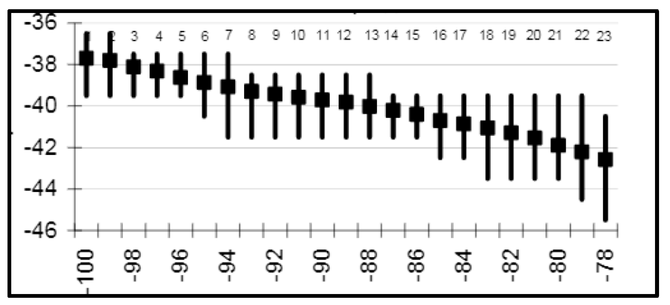
Figure 17.
Average catches of T. murphyi per trawling operation versus latitude and SST during austral winter 2020 (mid-August through early October) in the vicinity of the STF off central Chile (23–29° S, 74–76° W). All latitudes are rounded down; for example, 23 means the 23.00–23.99 range. Modified after Dubishchuk ([58], Figure 4).

Figure 18.
Long-term annual mean sea surface salinity (SSS) (top) and SSS gradient magnitude GM (bottom) from SMOS satellite data, 2012–2019.
Figure 18.
Long-term annual mean sea surface salinity (SSS) (top) and SSS gradient magnitude GM (bottom) from SMOS satellite data, 2012–2019.


Table 1.
Remote sensing studies of the STFZ in the Southeast Pacific. *, Var., Variable; MCSST, Multi-channel SST.
Table 1.
Remote sensing studies of the STFZ in the Southeast Pacific. *, Var., Variable; MCSST, Multi-channel SST.
| Authors, Year, Reference Number | Var. * | Sensor; Satellite | Period | Region | Resolution |
|---|---|---|---|---|---|
| Artamonov, Skripaleva 2006 [21] | SST | AVHRR | 1985–2002 | 84° W | 54 km, 1 mo. |
| Artamonov, Skripaleva 2008 [22] | SST | AVHRR | 1985–2002 | 140° W–72° W | 54 km, 1 mo. |
| Artamonov et al. 2009 [23] | SST | AVHRR | 1985–2002 | S. Ocean | 54 km, 1 mo. |
| Gordeeva, Malinin 2006 [24] | SST | Misc. | 1982–2003 | 100° W–77° W | 111 km, 1 mo. |
| Krasnoborodko 2017 [25] | SST | Misc. | 1971–2000 | 170° W–85° W | 111 km, 1 mo. |
| Lebedev, Sirota 2007 [26] | SSH | TOPEX/Poseidon | 1992–2003 | 110° W–80° W | 111 km, 1 day |
| Lebedev, Sirota 2007 [26] | SST | MCSST * | 1992–2003 | 110° W–80° W | 18 km, 1 week |
| Malinin, Gordeeva 2009 [27] | SST | Misc. | 1982–2006 | 100° W–77° W | 111 km, 1 mo. |
| Sirota et al. 2004 [28] | SSH | TOPEX/Poseidon | 1992–2003 | 109° W–90° W | 111 km, 1 day |
Disclaimer/Publisher’s Note: The statements, opinions and data contained in all publications are solely those of the individual author(s) and contributor(s) and not of MDPI and/or the editor(s). MDPI and/or the editor(s) disclaim responsibility for any injury to people or property resulting from any ideas, methods, instructions or products referred to in the content. |
© 2023 by the authors. Licensee MDPI, Basel, Switzerland. This article is an open access article distributed under the terms and conditions of the Creative Commons Attribution (CC BY) license (https://creativecommons.org/licenses/by/4.0/).
Share and Cite
MDPI and ACS Style
Belkin, I.M.; Shen, X.-T. Remote Sensing of the Subtropical Front in the Southeast Pacific and the Ecology of Chilean Jack Mackerel Trachurus murphyi. Fishes 2023, 8, 29. https://doi.org/10.3390/fishes8010029
AMA Style
Belkin IM, Shen X-T. Remote Sensing of the Subtropical Front in the Southeast Pacific and the Ecology of Chilean Jack Mackerel Trachurus murphyi. Fishes. 2023; 8(1):29. https://doi.org/10.3390/fishes8010029
Chicago/Turabian StyleBelkin, Igor M., and Xin-Tang Shen. 2023. "Remote Sensing of the Subtropical Front in the Southeast Pacific and the Ecology of Chilean Jack Mackerel Trachurus murphyi" Fishes 8, no. 1: 29. https://doi.org/10.3390/fishes8010029