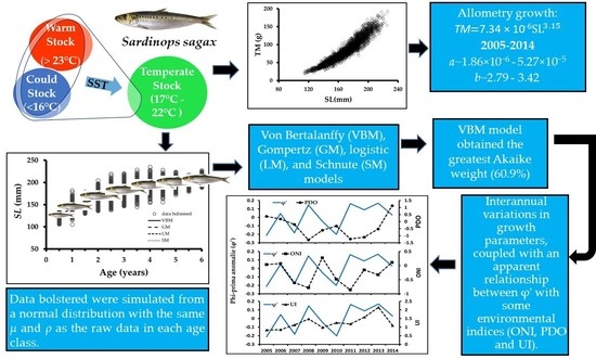
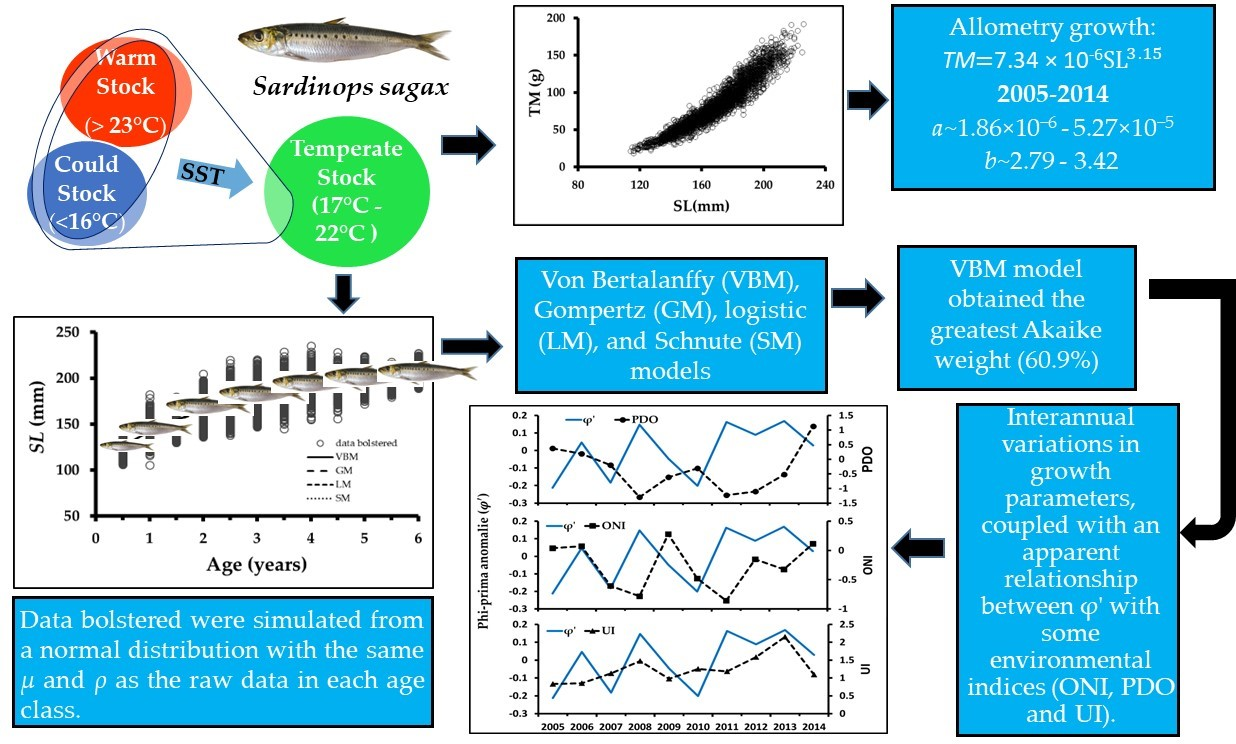
Allometry and Individual Growth of the Temperate Pacific Sardine (Sardinops sagax) Stock in the Southern California Current System

Abstract

We analyzed individual growth and body mass allometry of the temperate stock of Sardinops sagax from samples collected on commercial fleet during 2005 to 2014 in the southern California Current System. Ages were estimated on otolith growth ring reading. Age (years) and standard length (SL; mm) data were fitted using four growth models: von Bertalanffy (VBM), Gompertz (GM), logistic (LM), and Schnute (SM) models. Parameters of each model were calculated by the maximum likelihood method using Akaike information criterion and Akaike’s weight (WAIC_i) to select the model with the greatest plausibility. Additionally, the interannual growth performance (φ′) variation was described. Body mass allometry was established from the relationship between total body mass (TM; g) and standard length. The sardine samples ranged in size from 114 to 226 mm SL and in weight from 20 to 192 g TM; ages varied from 0.5 to 6.0 years. The allometric parameter (b) was estimated to be 3.155 (3.154–3.156), showing a hyper-allometry growth type. On the basis of raw data, we found that the LM model fit the original data better (WAIC_i ~35%). When models were fitted to data bolstered with simulated values, the VBM model obtained the greatest weight (WAIC_i = 60.9%), but the LM model had null plausibility. Consequently, we determined that the Pacific sardine growth pattern was best described by the VBM model, which appears to be more robust against biased data. The φ′ showed interannual variation (2.13–2.51), with an average of φ′ = 2.25. An apparent inverse relationship was observed between φ′ and the Oceanic Niño Index (ONI) or the Pacific Decadal Oscillation (PDO) and the apparent positive relationship between Upwelling Index (UI) and φ’.

1. Introduction

The Pacific sardine Sardinops sagax (Jenyns, 1842)—a resource that has supported one of the most important fisheries in the California Current System (CCS) [1,2]—has frequently been the dominant species among small pelagic fishes throughout the CCS [3,4,5]. The species is distributed from Alaska, USA, to Baja California Sur, Mexico, and within the Gulf of California [4,6]. Three stocks of this species have been hypothesized—cold, temperate, and warm—overlaid dynamically in space, exhibiting temporal asynchrony influenced by sea surface temperature (SST) variability within the CCS. The cold or northern stock inhabits waters from 13 °C to 17 °C, extending from Ensenada (EN), Baja California (BC), México, to San Pedro (SP), California, USA, from January to June and from Oregon, USA, to British Columbia, Canada, from July to December. The temperate or southern stock is adapted to temperatures from 17 °C to 22 °C, located off BC and SP from October to December and from April to June off Bahía Magdalena (MB), Baja California Sur (BCS) up to the middle part of BC (Figure 1). The warm stock adapted to temperatures that oscillate from 22 °C to 27 °C inhabits the Gulf of California with seasonal migrations off Bahia Magdalena from July to December [7,8,9,10,11,12].

Due to the catch volumes, this small pelagic fishery is the most important in Mexico since it provides up to 50% of national fishery and aquaculture production [13]. In the last decade, an annual average of 678,031 tons of small pelagic fish has been reported, where the Pacific sardine has represented 38% on average.

According to previous studies, fluctuations in the S. sagax biomass may be due to environmental factors that influence variability in population parameters [8,12,14].

Furthermore, parameter variation in time and space, such as individual growth, may be due to ecosystem dynamics [15]. To make an adequate evaluation of any fish stock subjected to exploitation, detailed estimation of individual growth is necessary [16,17,18]. Some growth parameters, such as allometry ($b$), individual growth coefficient (k), and asymptotic length (L_∞), are used as seed values in integrated models [19,20], which serve to estimate the current state of the exploited fish population.

For S. sagax, as in most fish populations, the von Bertalanffy growth model (VBM) has been the most used for individual growth description [15,21,22,23,24,25,26]. Other functions frequently used are Gompertz, logistic [27], Schnute [28], and Schnute–Richards [29] models. The Akaike information criterion (AIC), framed in the information theory approach, has been used to evaluate the performance of the models and to select the one with the greatest biological and statistical plausibility [18,25,26,30].

Even though studies on the growth of the Pacific sardine have been conducted [21,23,31], in these studies, only fish caught in Bahía Magdalena or Isla Cedros from the temperate stock were evaluated. However, there is no updated evaluation of the growth of the entire temperate stock, i.e., one that includes information on the sardines caught between Ensenada and Bahía Magdalena. Therefore, in this study, the body mass allometry and individual growth of the temperate stock of Pacific sardine in the southern CCS were analyzed through the information theory approach to select the model that best represents the somatic growth for this species. This was evaluated using the VBM, Gompertz, Schnute, and logistic models. Additionally, we examined whether there are interannual variations in growth parameters, and the possible relationship between growth performance and the environment is discussed.

2. Materials and Methods

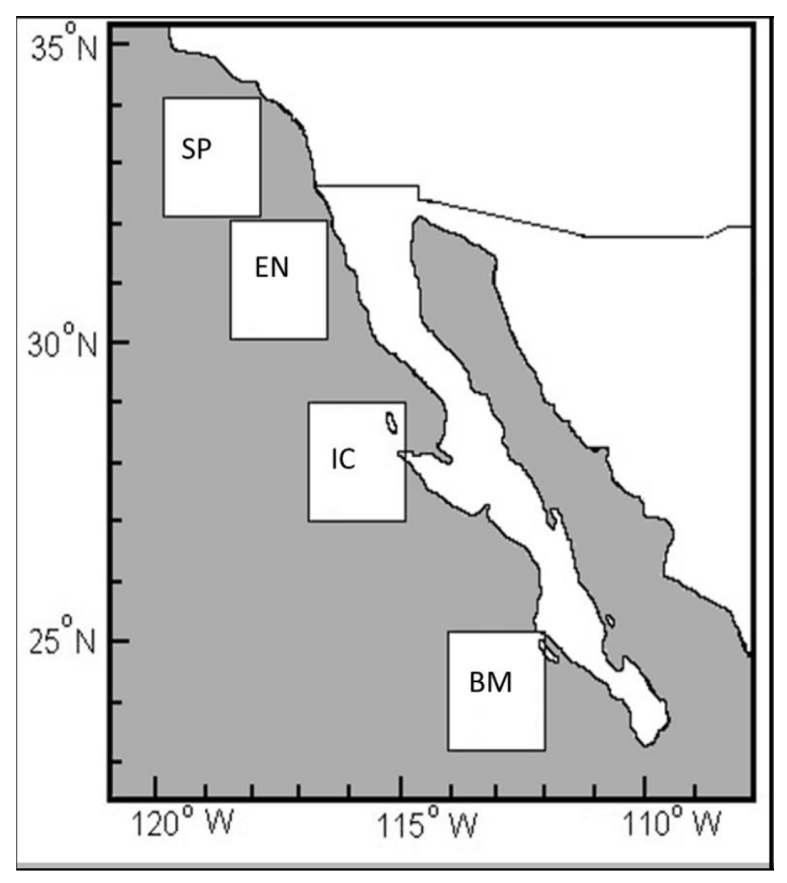
2.1. Study Area

The purse-seine fishing fleet carries out its sardine fishing activities along the coast of the Baja California peninsula, Mexico (Figure 1), landing their catches both in Ensenada, BC, and in Bahia Magdalena, BCS. This region is influenced by interannual events (such as El Niño and La Niña) and has a seasonal upwelling regime in spring–summer. During El Niño events, warmer than average conditions occur, increasing the salinity, deepening the thermocline and nutricline, decreasing the primary productivity, and changing the composition of zooplankton species [32,33,34,35,36]. The reverse is observed during cold interannual events (La Niña) [33,36].

Figure 1. Map of the study area showing the distribution of the temperate stock Pacific sardine (Sardinops sagax). BM (Bahía Magdalena); IC (Isla Cedros); EN (Ensenada); SP (San Pedro).

Figure 1. Map of the study area showing the distribution of the temperate stock Pacific sardine (Sardinops sagax). BM (Bahía Magdalena); IC (Isla Cedros); EN (Ensenada); SP (San Pedro).

2.2. Data Collection

Data were taken from the small pelagic monitoring programs of Instituto Nacional de Pesca y Acuacultura (INAPESCA) and Centro Interdisciplinario de Ciencias Marinas (CICIMAR) collected from 2005 to 2014. By law, the purse-seine nets for sardine capture have a maximum length of 640 meters, with a mesh size of 25 mm. Since the fishing fleet carries out its fishing activities all year round, the sampling was performed throughout the year at the landing ports (Ensenada and Bahia Magdalena). To have a better representation of the temperate stock, a sample of approximately 10 kg (from 80 to 100 sardines, depending on individual weight) was taken randomly; at least one sample per month per landing port of Pacific sardine was obtained. All sardines in the sample were measured for standard length (SL, precision ±1 mm) and grouped into 5 mm length intervals. Next, five sardines were randomly selected from each length interval or, if there were less than five, all sardines in that interval were selected. This subsample of fish was measured for biological characteristics such as standard length (SL) and total body mass (TM, precision of ± 1 g), and sagitta otoliths were removed.

2.3. Age Determination

Age was determined by counting the number of opaque and hyaline growth increments in the otoliths. For this, otoliths were mounted on glass slides with synthetic resin. A stereoscopic microscope (16× and 40×) was used with reflected light on a dark background to examine otoliths. Under these conditions, opaque (white color) and hyaline (dark color) growth increments were observed and counted [18,37,38]. The readings were made by two independent readers, and the results were compared (each otolith was read twice by each reader); in cases where a difference was found in the readings, the otoliths were reread simultaneously by the two readers and a joint decision was reached. The readers did not have previous information about each specimen’s SL.

The precision of age determinations between readers was evaluated by calculating the average percentage error (APE) [39] and coefficient of variation (CV) [40]. The formation periodicity of opaque and hyaline growth increments was determined through otolith edge graphical analysis [18,23,37].

We did not assume any birthdate for the Pacific sardine, because we know that this is a species that has partial reproduction and an extended reproductive period that can last up to 6 months. Therefore, we assigned ages to sardines as a function of the number of growth increments counted in the otolith: (1) if the otolith of a given sardine had three growth increments counted, one opaque, one hyaline, and the edge was undoubtedly opaque, this sardine was assigned an age of 1.5 years; (2) if the otolith of a given sardine had six growth increments counted, three opaque and three hyaline, and the edge was without undoubtedly hyaline, this sardine was assigned an age of 3.0 years; (3) if the otolith of a given sardine was counted nine growth increments, five opaque and four hyaline, with the edge being undoubtedly opaque, this sardine was assigned an age of 4.5 years. This approach was used in all otoliths.

2.4. Differentiating Sardinops sagax Stock Catches

In order to separate the three different stocks that inhabit the western coast of the Baja California peninsula, the differentiation criterion of stock catches by temperature was used [7]. Catch data from 2005 to 2014 were grouped monthly by collection area to define each stock component. This could be applied because each catch landed has the record of the area where the catch was made. The warm stock (WS) inhabits temperatures higher than 22 ℃, the temperate stock (TS) inhabits temperatures from 17 ℃ to 22 ℃, and the cold stock (CS) inhabits temperatures below 17 ℃. To obtain sea surface temperature (SST), we used the Geospatial Interactive Online Visualization and Analysis Infrastructure (Giovanni) system developed and maintained by the National Aeronautics and Space Administration (NASA), Goddard Earth Sciences (GES) Data and Information Services Center (DISC) (https://giovanni.gsfc.nasa.gov, accessed on 11 January 2021). Monthly averages of sea surface temperature (SST) were obtained by quadrants of 2° N × 2° W (Figure 1); those in Bahía Magdalena were from 23 to 25° N × 112 to 114° W, those in Isla de Cedros were from 27 to 29° N × 115 to 117° W, and those in Ensenada were from 30 to 32° N × 117 to 119° W [7].

2.5. Body Mass–Length Relationship

Body mass allometry was established from the relationship between total body mass (TM; g) and standard length (SL; mm), considering all sampled data (2005–2014), using the potential model [27].

$$TM=aS{L}^b,$$

(1)

where parameter b indicates the growth pattern, and a is a parameter describing body shape [41]. Adjustments were performed using the maximum log-likelihood function.

$$LL\left(\varphi |data\right)=-\frac{n}{2}\left[ln2\pi +2ln\sigma +1\right],$$

(2)

where $\varphi$ represents the model parameters, n is the sample size, and $\sigma$ is the standard deviation (SD), which was calculated and estimated considering a normal distribution of error.

$$\sigma =\sqrt{\frac{{\sum }_{i=1}^n{\left(T{M}_i-\widehat{TM}\right)}^2}{n}},$$

(3)

where TM_i is the total body mass observed, and $\widehat{TM}$ is the total body mass estimated.

The confidence intervals (95% CI) of parameters a and b were estimated [42] and used for comparing parameter b with b = 3 (isometry) [43] and defining growth type (b < 3, hypo-allometric or negative allometry; b > 3, hyper-allometric or positive allometry) [41].

2.6. Selecting the Best Fish Growth Model

Fish growth adjustment was performed using four growth models (

Table 1. Candidate growth models for the temperate Sardinops sagax stock age-at-length data in the southern California Current System (CCS).

Model	Equation	Description
VBM	$L\left(t\right)=L_{\infty }\left[1-e^{-k\left(t-t_0\right)}\right]$	$L\left(t\right)$ is size (in mm SL) at age t, $L_{\infty }$ is asymptotic length (mm SL), $k$ is the growth rate coefficient (year−1), $t_0$ in VBM and SM is the theoretical age at which length is zero (years). $t_0$ in GM and LM corresponds to an inflection point on the growth curve $t$ is age at size $L\left(t\right)$ $\pi$ is a relative growth rate (time constant) $\mathit{\lambda }$ is an incremental relative growth rate (incremental time constant), $T_1$ is the lowest age in the dataset,$T_2$ is the highest age in the dataset, $L_1$ is the size at age $T_1$, $L_2$ is the size at age $T_2$
GM	$L\left(t\right)=L_{\infty }{e}^{\left(-\left(\frac{1}{k}\right)e^{-k\left(t-t_0\right)}\right)}$
LM	$L\left(t\right)=L_{\infty }{\left[1-e^{-K\left(t-t_0\right)}\right]}^{-1}$
SM	$L\left(t\right)={\left[L_1{}^{\pi }+\left(L_2{}^{\pi }-L_1{}^{\pi }\right)\frac{1-e^{-\mathit{\lambda }\left(t-T_1\right)}}{1-e^{-\mathit{\lambda }\left(T_2-T_1\right)}}\right]}^{\frac{1}{\pi }}$

): the von Bertalanffy growth model (VBM) [44], the Gompertz growth model (GM) [45], the logistic model (LM) [27], and the Schnute model (SM) [28]. The Schnute model was used assuming that the parameters ʎ and π are not equal to zero [28].

The parameters of each model were estimated assuming that the residuals had a log-normal distribution around the growth models. For all candidate growth models, the parameters ($\theta$) were fitted maximizing the log-likelihood function through an iterative procedure with Newton’s algorithm [20,46].

$$L{L}_{\left(\theta |data\right)}=-\left(\frac{n}{2}\right)\left(ln\left(2\pi \right)+2\times ln\left(\sigma \right)+1\right),$$

(4)

where LL_(ϕ|data) is the maximum log-likelihood value, n is the sample size, and σ is the standard deviation (SD), which was obtained using the following analytical equation [20]:

$$\sigma =\sqrt{\frac{{\sum }_{i=1}^n{\left(ln\left(S{L}_{obs\left(t\right)i}\right)-ln\left(S{L}_{est\left(t\right)}\right)\right)}^2}{n}},$$

(5)

where $S{L}_{obs\left(t\right)i}$ is the standard length observed (in mm) at age $t$ (in years), and $S{L}_{est\left(t\right)}$ is the estimated standard length at age $t$. It was assumed that $L\left(t\right)$ had a log-normal distribution around the candidate growth models. The objective function was solved using Solver in Excel^®.

The Akaike information criterion (AIC) [25,26,30] was used to select the best growth model for the S. sagax age and length data according to the following equation:

$$AIC=\left(-2L{L}_{\left(\theta |data\right)}\right)+2K,$$

(6)

where K denotes the total estimated parameters, including σ [30]. The AIC differences (Δi) for each model were given by the following function:

$$\mathsf{\Delta }i=AICi–AICmin,$$

(7)

where AICmin represents the AIC for the best candidate growth model, and AIC_i is the AICmin estimated for each growth model. Plausibility was estimated for candidate ($i$) by means of Akaike weight (WAIC_i), providing a proportional best adjustment index according to the following equation [30]:

$$WAI{C}_i=\frac{e^{-0.5\Delta i}}{{\sum }_{i=1}^4{e}^{-0.5\Delta i}}.$$

(8)

The parameter ($\theta$) confidence intervals (CI) were estimated using profile likelihood construction [47,48]. A likelihood interval by itself is not very informative and, thus, insufficient to indicate change. A likelihood interval must always be accompanied by the value of $\theta$ to give some idea of the symmetry of the likelihood function with respect to probable alternative values of $\theta$ and, in this sense, show how plausibility changes within the interval. This estimation was made for all growth parameters, considering a distribution χ² with m degrees of freedom [49,50], where CIs were defined as all values $\theta$ that satisfied inequality.

$$\mathrm{CI}=2\left[LL\left(\theta |\mathrm{data}\right)-LL\left(\theta |best\right)\right]<{\chi }_{1,1-\alpha }^2,$$

(9)

where $LL\left(\theta |best\right)$ is the log-likelihood of the most probable value of θ, $LL\left(\theta |data\right)$ is the log-likelihood θ within the likelihood profile, and ${\chi }_{1,1-\alpha }^2$ projects the distribution of χ² with one degree of freedom at a confidence level of 1 − α. Thus, the 95% CI includes all the values of θ that double the difference between the log-likelihood in the likelihood profile and the best estimate of θ, i.e., all values less than 3.84 were included in CI [20,51].

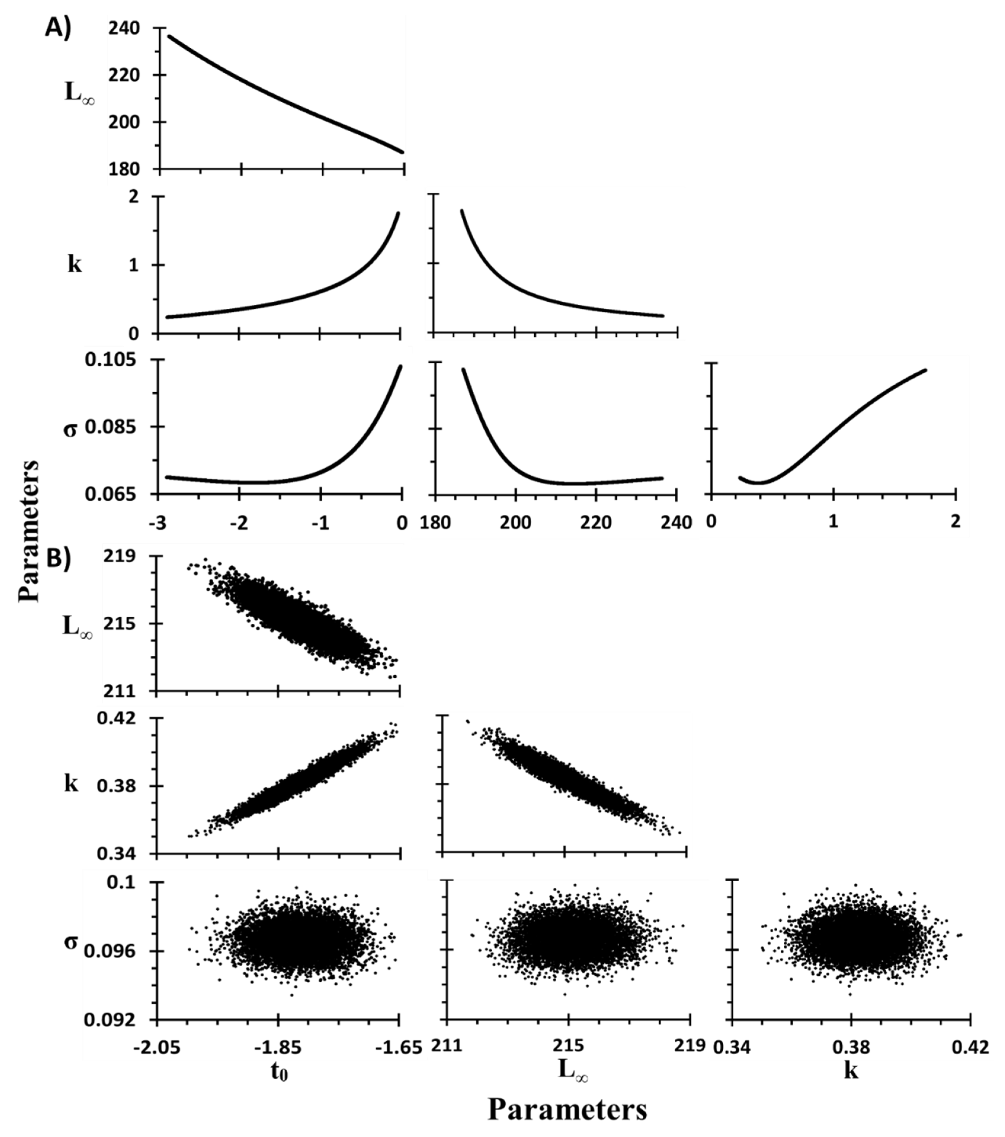
2.7. Sensitivity Analysis

A sensitivity analysis was performed to quantify the effect of the sampled distribution on the growth parameter estimates following the approach of Bolser et al. [52] and Scherrer et al. [53]. For this, different amounts of simulated data were added to the original data, such that each observed age (0.5 to 6.0 years) had 500 observations to compensate for unequal sampling between age groups. In the case of ages 2.0 and 3.0 years, data were not simulated because these ages had 1090 and 640 data, respectively; therefore, in these two cases, 500 data were randomly selected from the raw data. The data were simulated from a normal distribution with the same mean and standard deviation as the raw data in each age class. The normality of the data distributions was tested using the Kolmogorov–Smirnov statistical test. Each model was then fitted using this new dataset, and the goodness of fit was assessed in the same way as described above. Bolser et al. [52] and Scherrer et al. [53] highlighted that this type of approach does not explicitly consider differences in selectivity or differences between the structure of the sampled and the true population but can fill critical gaps caused by these and other factors [54,55] by homogenizing the number of observations of each of the age–size classes.

2.7.1. Sensitivity in Growth Parameters of VBM

Additionally, we calculated the bias in k and L_∞ of VBM through a comparison between the two- and three-parameter estimation models, following Pardo et al. [56].

2.7.2. Model VBM—Three Parameters (VBM-3)

A von Bertalanffy growth curve was created with the following parameters: k = 0.383 year⁻¹, L_∞ = 214.6 mm, and t₀ = −1.813 years; to simulate the uncertainty in size-at-age values, for each of the 12 age classes, we drew 1000 random draws from a log-normal distribution with mean-centered bias correction [56].

$$L_{te}=L_{tor}\times e^{\mathsf{{\rm N}}\left(\mu ,\sigma \right)+\frac{{\sigma }^2}{2}},$$

(10)

where $L_{te}$ is the distribution of length-at-age t with error included, $L_{tor}$ is the length-at-age $t$ of the original model, and Ν (μ, σ) is a normal distribution with a mean of 0 (μ) and standard deviation (σ) of 0.1. The set of 12,000 simulated data $L_{te}$ replace the original length-at-age values, and the parameters $t_0$, $k$, and $L_{\infty }$ were estimated using the maximum likelihood function, assuming that the residual errors are of the multiplicative type (Equations (4) and (5)).

2.7.3. Model VBM—Two Parameters (VBM-2)

The methodology described by Neer et al. [57] was used, where $t_0$ is fixed iteratively from a normal distribution of possible ages at which length is zero for Pacific sardine obtained from bibliographic sources (−0.02 to −2.88) [12,18,31]. Once $t_0$ was fixed, the parameters k and $L_{\infty }$ were estimated considering the 12,000 values of length-at-age using the maximum likelihood function, assuming that the residual errors are of the multiplicative type (Equations (4) and (5)).

2.7.4. Estimation of Parameters and Confidence Intervals

Both models (VBM—two parameters and VBM—three parameters) were run 10,000 times, creating in each process a new dataset that was used to describe the empirical distribution of the parameters. The values of the mean ($\tilde{x})$ and standard deviation (SD) of the bootstrap are considered as an estimate of the mean value and standard error of θ. The coefficient of variation (CV) was estimated as $CV=\raisebox{1ex}{$SD$}\!\left/ \!\raisebox{-1ex}{$\tilde{x}$}\right.$ [58]. The bias (B) and percentage bias (%B) were estimated as follows: $B=\tilde{x}-\theta$ and $\%B=\frac{\tilde{x}-\theta }{\theta }\times 100\%$ [59], where $\theta$ is the i-th best estimate of the parameters of the proposed model. Confidence intervals were calculated using the bias-corrected percentile method [20].

2.8. Annual Growth (2005–2014)

To determine if there were variations in growth between the years 2005 and 2014, the VBM model was adjusted to the bolstered raw data of each year, estimating the growth parameters using the maximum likelihood function, assuming that the residual errors are of the multiplicative type (Equations (4) and (5)). On the basis of the results of this analysis, growth performance was evaluated using the phi-prime (φ′) index proposed by Pauly and Munro [60]. This index reflects the relationship between $L_{\infty }$ (the theoretical maximum length) and k (the growth coefficient) of VBM. Phi-prime was estimated using the following equation:

$${\phi }^{\prime }={\log }_{10}k+2{\log }_{10}{L}_{\infty }.$$

(11)

To highlight the differences from the average, the φ′ anomalies were obtained as

$$anom={{\phi }^{\prime }}_i-\left[\frac{{\sum }_{i=1}^n{\phi }^{\prime }}{n}\right],$$

(12)

where i is the year, φ′_i is the growth performance index, and n is the total number of years.

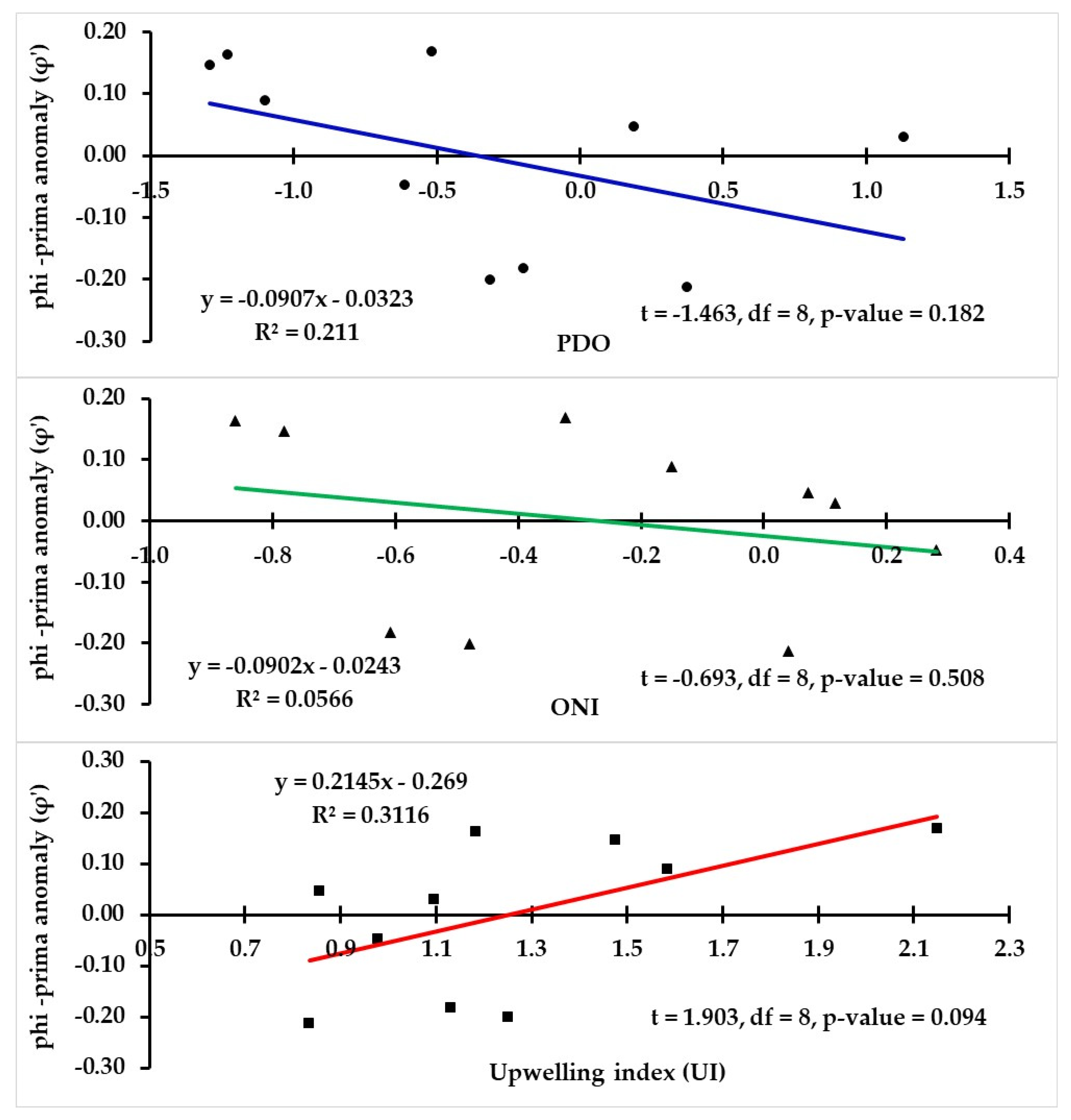
2.9. Relationship between Individual Growth and Environmental Conditions

The interannual relationships of the individual growth of the temperate stock of S. sagax (φ′) with environmental variables such as the Pacific Decadal Oscillation (PDO, httph://www.ncei.noaa.gov/pub/data/cmb/ersst/v5/index/ersst.v5.pdo, accessed on 6 February 2021), the Oceanic El Niño Index (ONI, https://psl.noaa.gov/data/correlation/oni, accessed on 11 February 2021), and the Upwelling Index (UI, https://www.pfeg.noaa.gov/products/PFELData/upwell/monthly/upindex.mon, accessed on 14 February 2021), were analyzed through a simple linear regression analysis and using Pearson’s correlation test.

3. Results

3.1. Differentiating of Sardinops sagax Stock Catches

Of the total landings of S. sagax captured on the western coast of the Baja California peninsula during the period from 2005 to 2014, on average 66% belonged to the temperate stock (17 °C–22 °C), 21% corresponded to the warm stock (>22 °C), and 13% corresponded to the cold stock (<17 °C). For the following analysis, only information from the temperate stock of S. sagax from the southern part California Current was used.

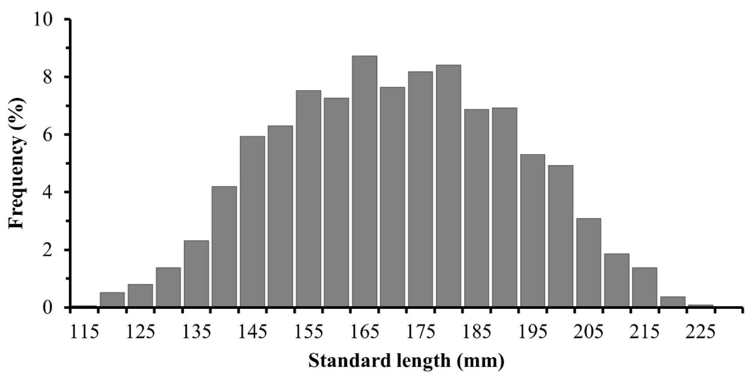
3.2. Structure of Standard Lengths

A total of 3509 fish were analyzed from 2005 to 2014 along the distribution area of temperate S. sagax stock. The SL frequency distribution (Figure 2) for all seasons combined (2005–2014) showed a length range from 114 to 226 mm of SL, with an average of 169.1 mm SL and SD at 21.07 mm; in weight, the sardines ranged between 20 and 192 g of TM (mean: 82.94 ± 32.77 g). The length frequency distributions and ages for each year are presented in the Figure S1 and Figure S2, respectively (Supplementary Materials). It was observed that there were differences between years, with some years presenting very few small fish (or young ages) and others with fewer large fish (or older).

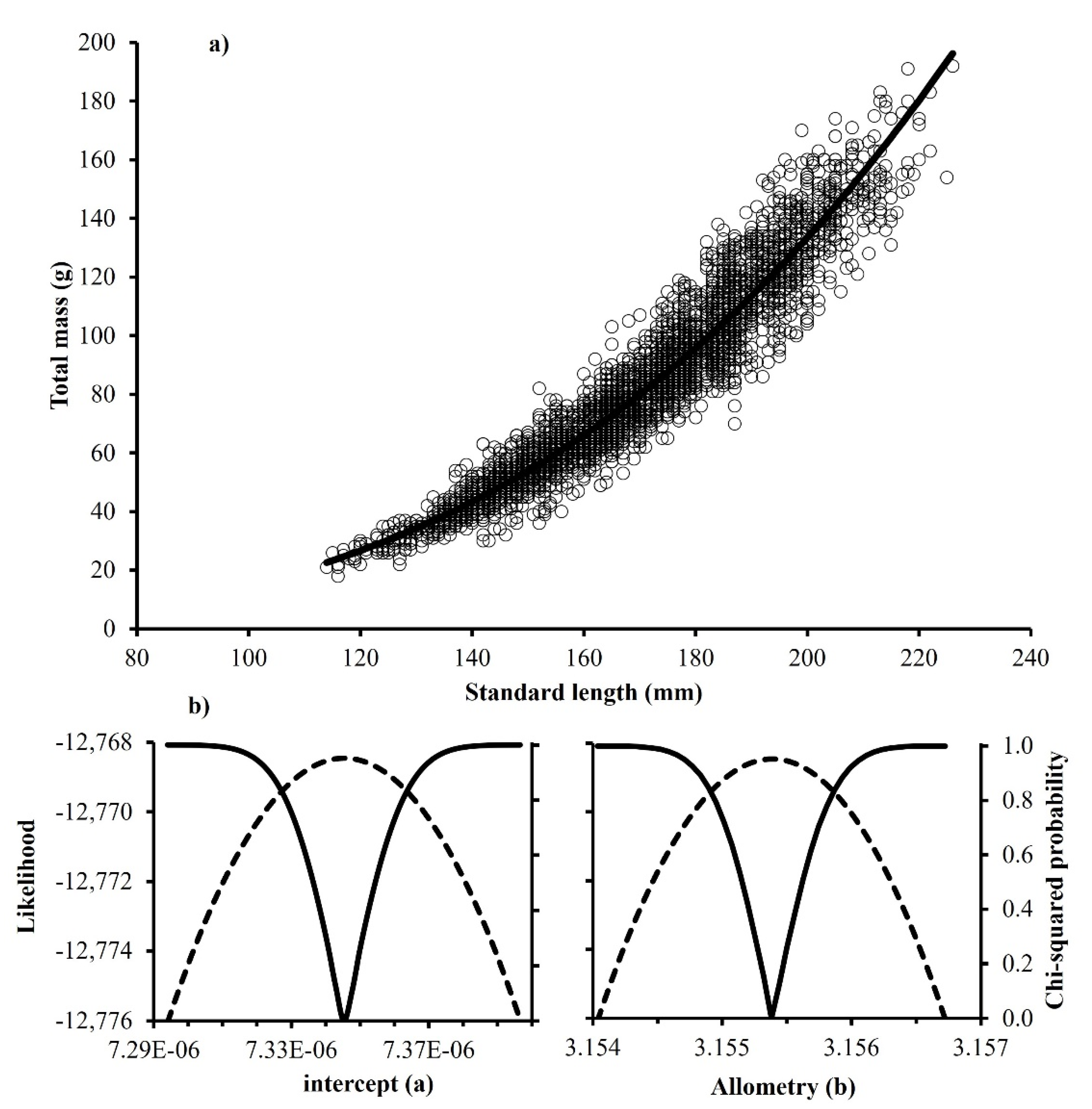
3.3. Body Mass–Length Relationship

Figure 3a shows all data from 2005 to 2014 and the relationship between TM and SL. The parameters a and b obtained with respective confidence profiles are shown in Figure 3b. An intercept value of a = 7.34 × 10⁻⁶ was obtained with a 95% CI between 7.32 × 10⁻⁶ and 7.37 × 10⁻⁶. The value obtained for b = 3.155 showed a hyper-allometry (+H) growth type. This, considering the range of the 95% CI between b = 3.154 and 3.156, does not include the value of 3.0. When evaluating the TM–SL relationship for each year from 2005 to 2014 (

Table 2. Average values and 95% confidence intervals (CI; α = 0.05) of parameters a and b obtained by adjusting the potential model for each year from 2005 to 2014, including all data (average) of the temperate Sardinops sagax stock and growth type (GT; +H, hyper-allometry; −H, hypo-allometry).

Year	a			b			n	GT
	CIinf	Mean	CIsup	CIinf	Mean	CIsup
2005	3.218 × 10−6	3.242 × 10−6	3.281 × 10−6	3.319	3.321	3.323	463	+H
2006	1.710 × 10−5	1.742 × 10−5	1.773 × 10−5	2.982	2.986	2.989	164	+H
2007	9.194 × 10−6	9.209 × 10−6	9.302 × 10−6	3.103	3.104	3.106	550	+H
2008	2.841 × 10−5	2.869 × 10−5	2.896 × 10−5	2.890	2.892	2.893	392	−H
2009	1.835 × 10−6	1.861 × 10−6	1.876 × 10−6	3.419	3.421	3.423	215	+H
2010	3.755 × 10−5	3.800 × 10−5	3.845× 10−5	2.833	2.835	2.838	214	−H
2011	1.297 × 10−5	1.309 × 10−5	1.322 × 10−5	3.051	3.053	3.055	285	+H
2012	5.230 × 10−5	5.274 × 10−5	5.319 × 10−5	2.788	2.790	2.791	444	−H
2013	4.234 × 10−6	4.269 × 10−6	4.328 × 10−6	3.252	3.254	3.256	358	+H
2014	1.574 × 10−5	1.588 × 10−5	1.601 × 10−5	2.991	2.992	2.994	424	−H
2005–2014	7.32 × 10−6	7.34 × 10−6	7.37 × 10−6	3.154	3.155	3.156	3509	+H

), it was found that the a value varied from 1.86 × 10⁻⁶ to 5.27 × 10⁻⁵, and the b parameters showed values from 2.790 to 3.421, alternating between hyper-allometric and hypo-allometric (−H) growth types throughout the decade assessed (Table 2). The parameters of the relationship between TM and SL for each year from 2005 to 2014 are presented graphically in Figure 4. The TM–SL relationship adjusted to bolstered raw data is included in the Supplementary Materials (Table S1). The same behavior was observed in the values of parameters a and b, presenting hyper-allometric or hypo-allometric growth patterns in the same years.

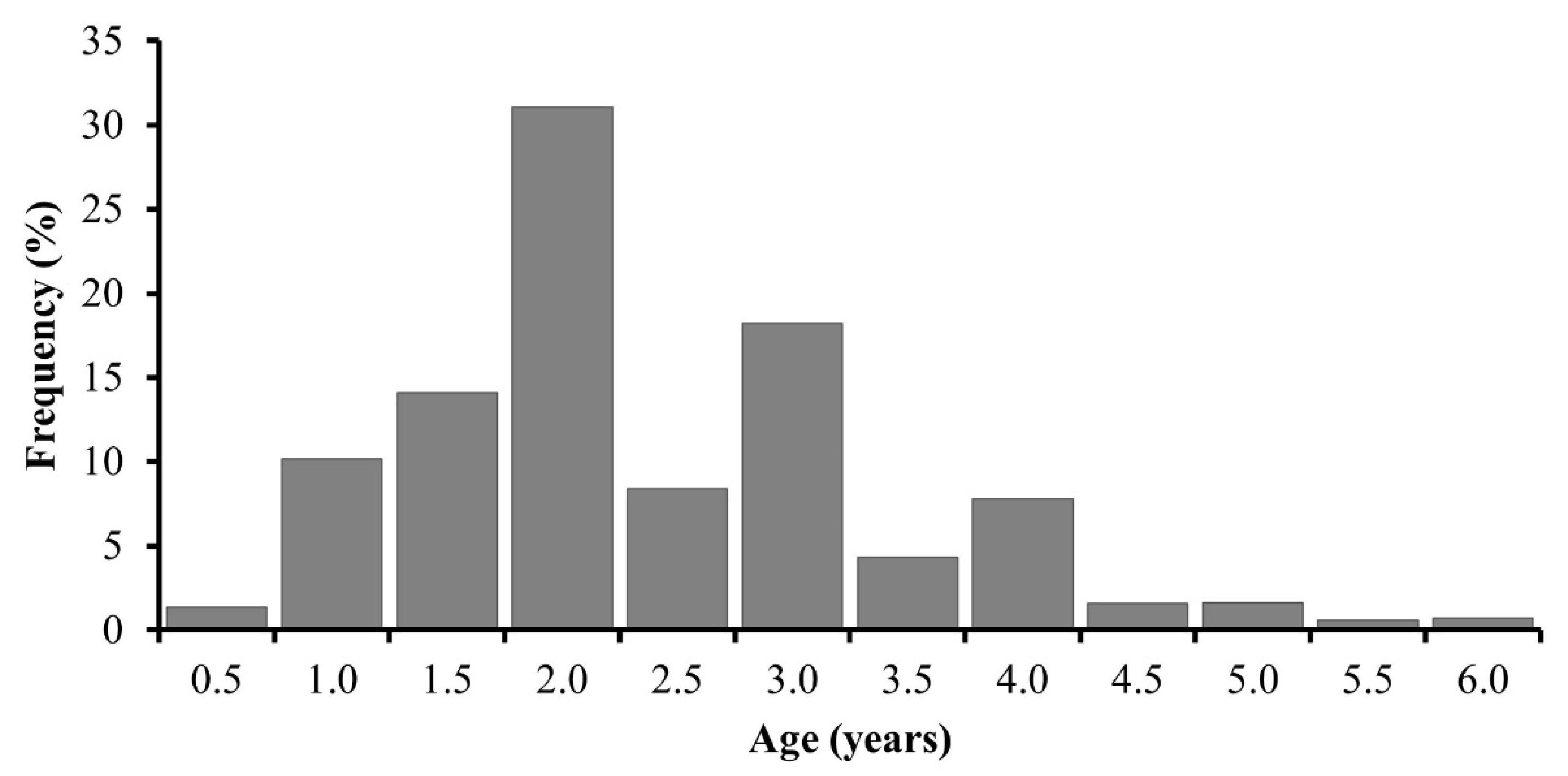
3.4. Age Determination

The average value of the percentage error (APE = 3.2%) and the average coefficient of variation (CV = 4.1%) indicated a good level of aging precision in the readings, which means reproducibility in the age determination between the readers. The edge analysis (Figure 5) highlighted the deposition of an opaque increment during the late spring–summer months, while a hyaline increment formed in the autumn–winter months, thus confirming an annual pattern of increasing deposition of opaque and hyaline increments.

Figure 6 shows the age structure, in which 12 age groups were found, fish from 0.5 years (one opaque edge) to 6.0 years (six opaque edges and six hyaline edges) of age. The highest frequency was observed at the age of 2 and 3 years. The average age was 2.39 years, and the standard deviation was 1.03 years.

Table 3. Mean standard length (SL, mm) at age and standard deviation (SD) determined for the temperate Sardinops sagax stock in the southern California Current System (CCS) during the study period (2005–2014) (n: sampling size).

Age	SL	SD	n
0.5	125.7	6.9	48
1.0	143.8	11.8	357
1.5	152.3	11.4	495
2.0	165.2	14.2	1090
2.5	175.5	14.7	295
3.0	182.0	15.1	640
3.5	186.8	13.3	152
4.0	192.0	13.1	274
4.5	193.9	10.3	55
5.0	199.2	9.8	57
5.5	199.4	6.5	21
6.0	206.4	6.8	25

shows the mean standard length at age and the corresponding standard deviation (SD) determined for the Pacific sardine temperate stock for all data from the period 2005 to 2014.

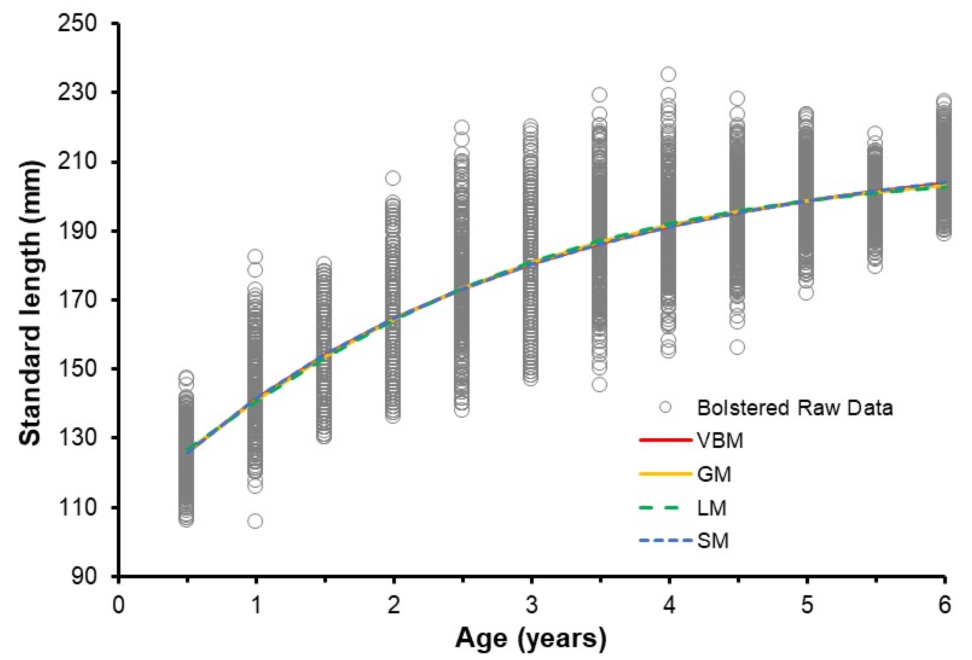
3.5. Selecting the Best Growth Model

The values of the growth parameters with their 95% CI for each model adjusted to the raw data are presented in

Table 4. Growth parameters values and 95% confidence intervals (CI; α = 0.05) estimated by models VBM (von Bertalanffy growth model), GM (Gompertz model), LM (logistic model), and SM (Schnute model), fitted to raw age–length data of the temperate Sardinops sagax stock in the southern California Current System (CCS) during the study period (2005–2014).

Model	Parameter	Value	Lower CI	Upper CI
VBM	$t_0$ (year)	−1.845	−1.870	−1.821
	$L_{\infty }$ (mm)	216.3	215.6	217.1
	$k$ (year−1)	0.372	0.369	0.375
GM	$t_0$ (year)	−0.906	−0.934	−0.880
	$L_{\infty }$ (mm)	211.0	210.4	211.7
	$k$ (year−1)	0.479	0.474	0.483
LM	$t_0$ (year)	−0.296	−0.324	−0.269
	$L_{\infty }$ (mm)	207.4	206.7	208.1
	$k$ (year−1)	0.586	0.578	0.593
SM	$\mathit{\lambda }$	0.536	0.523	0.344
	$\pi$	−0.538	−0.685	1.574
	$L_1$ (mm)	127.1	126.3	127.9
	$L_2$ (mm)	202.8	201.8	204.0

For SM, $L_{\infty }$ = 208.9 mm and $t_0$ = −1.71 years.

. Estimated L_∞ varied between 207.4 mm and 216.3 mm SL, while the estimated k varied between 0.372 and 0.586 year⁻¹, with the lowest value estimated for VBM and highest values estimated for the other models (Table 4). The estimated values for AICi, Δi, and WAIC_i of each evaluated model are presented in

Table 5. Growth model selection for models fitted to raw age-length data of the temperate Sardinops sagax stock in the southern California Current System (CCS). K is the number of parameters; LL is the maximum log-likelihood; AIC is the Akaike’s information criterion; Δi is Akaike’s differences; WAIC_i% is Akaike’s weight for each model; SE is the standard error.

Model	K	LL	AIC	Δi	WAICi%	SE
VBM	4	3864.11	−7720.23	1.290	18.15	0.08
GL	4	3864.73	−7721.47	0.049	33.77	0.08
LM	4	3864.76	−7721.52	0.000	34.61	0.08
SM	5	3864.82	−7719.63	1.886	13.47	0.08

. All the compared models had a value of Δ < 2, while the WAIC varied between 13.47% and 34.61%, which indicates that all models were substantially supported by the data. It is shown in Figure S3 (Supplementary Materials) that the growth models produced similar asymptotic growth patterns.

The assumption that the length-at-age data were normally distributed could not be rejected on the basis of the Kolmogorov–Smirnov test. This diagnostic indicated that the data simulation approach was adequate.

Table 6. Growth parameter values and 95% confidence intervals (CI; α = 0.05) estimated by models VBM (von Bertalanffy growth model), GM (Gompertz model), LM (logistic model), and SM (Schnute model), fitted to raw age–length data bolstered by simulated values of the temperate Sardinops sagax stock in the southern California Current System (CCS) during the study period (2005–2014).

Model	Parameter	Value	Lower CI	Upper CI
VBM	$t_0$ (year)	−1.813	−1.828	−1.799
	$L_{\infty }$ (mm)	214.6	214.2	215.0
	$k$ (year−1)	0.383	0.381	0.384
GM	$t_0$ (year)	−0.889	−0.904	−0.874
	$L_{\infty }$ (mm)	210.6	210.3	211.0
	$k$ (year−1)	0.484	0.481	0.487
LM	$t_0$ (year)	−0.262	−0.278	−0.247
	$L_{\infty }$ (mm)	207.9	207.5	208.2
	$k$ (year−1)	0.587	0.582	0.592
SM	$\mathit{\lambda }$	0.335	0.326	0.344
	$\pi$	1.474	1.378	1.574
	$L_1$ (mm)	125.8	125.3	126.4
	$L_2$ (mm)	204.1	203.6	204.5

For SM, $L_{\infty }$ = 217.1 mm and $t_0$ = −1.271 years.

shows the parameter estimates for the four models adjusted to the bolstered raw data, including their 95% CI. Estimated L_∞ varied between 207.9 mm and 217.1 mm SL, while the estimated k varied between 0.372 and 0.586 year⁻¹, with the lowest values estimated for SM and VBM and highest values estimated for LM and GM. The four models reflect a phase of rapid growth during the first 2 years of age (~80% $L_{\infty }$ value) and a growth rate decreasing after 4 years of age (~90% $L_{\infty }$ value) (Figure 7).

In

Table 7. Growth model selection for models fitted to raw age–length data bolstered by simulated values of the temperate Sardinops sagax stock in the southern California Current System (CCS). K is the number of parameters; LL is the maximum log likelihood; AIC is Akaike’s information criterion; Δi is Akaike’s differences; WAIC_i% is Akaike’s weight for each model; SE is the standard error.

Model	K	LL	AIC	Δi	WAICi%	SE
VBM	4	7590.59	−15,173.18	0.00	60.92	0.07
GM	4	7586.12	−15,164.24	8.94	0.70	0.07
LM	4	7577.67	−15,147.33	25.85	0.00	0.07
SM	5	7591.13	−15,172.25	0.92	38.38	0.07

, the estimated values for AICi, Δi, and WAICi according to the bolstered raw data for each evaluated model are presented. Only VBM and SM models had a value of Δ < 2, while the WAIC was 60.92% and 38.28%, which indicates that these two models were substantially supported by the data. The LM and GM received no support from Δ or WAIC (Table 7).

Synthesis of the above considerations and assessments led to the selection of the VBM as the best model to represent growth in the Pacific sardine temperate stock; in this sense, the parameters obtained from the VBM can be considered valid.

The Monte Carlo simulations revealing the covariation among the parameters estimated by the VBM of the Pacific sardine temperate stock considering VBM-2 and VBM-3 are shown in Figure 8A and Figure 8B, respectively. For both cases, $t_0$, $k$, and σ increased and $L_{\infty }$ decreased; if $L_{\infty }$ increased, $k$ and σ decreased, and, if $k$ increased, σ increased. Although the covariation scale for $t_0$ differed between both settings, this parameter was also relevant in the definition of growth for Pacific sardine temperate stock.

The descriptive statistics of the parameters estimated by Monte Carlo simulation and the 95% CI estimated by the bias-corrected percentile method are shown in

Table 8. Parameters and bias-corrected percentile confidence intervals (CI; α = 0.05) from von Bertalanffy model (VBM) for the temperate Sardinops sagax stock in the southern California Current System (CCS).

	Parameter	Value	Mean	SD	CV	Bias	%Bias	Lower CI	Upper CI
Two parameters (t0 fixed)	t0 (year)	−1.81	−1.45	0.83	−0.57	0.36	−19.84	−2.81	−0.09
	L∞ (mm)	214.60	209.77	13.74	0.07	−4.82	−2.25	188.72	235.00
	k (year−1)	0.38	0.58	0.34	0.59	0.20	52.11	0.27	1.71
	σ	0.07	0.07	0.01	0.11	0.01	7.83	0.07	0.10
Three parameters	t0 (year)	−1.81	−1.81	0.05	−0.03	0.00	0.02	−1.91	−1.73
	L∞ (mm)	214.60	215.11	0.94	0.00	0.51	0.24	213.34	217.06
	k (year−1)	0.38	0.38	0.01	0.02	0.00	0.02	0.37	0.40
	σ	0.07	0.10	0.00	0.01	0.03	41.50	0.10	0.10

. The parameters obtained by VBM-3 revealed lower CV and biases than estimated by VBM-2, where the mean values estimated by VBM-3 were close to the parameters estimated via the objective maximum likelihood function. These results reveal that the 95% CI for the estimated parameters by VBM-3 had more accuracy (Table 8).

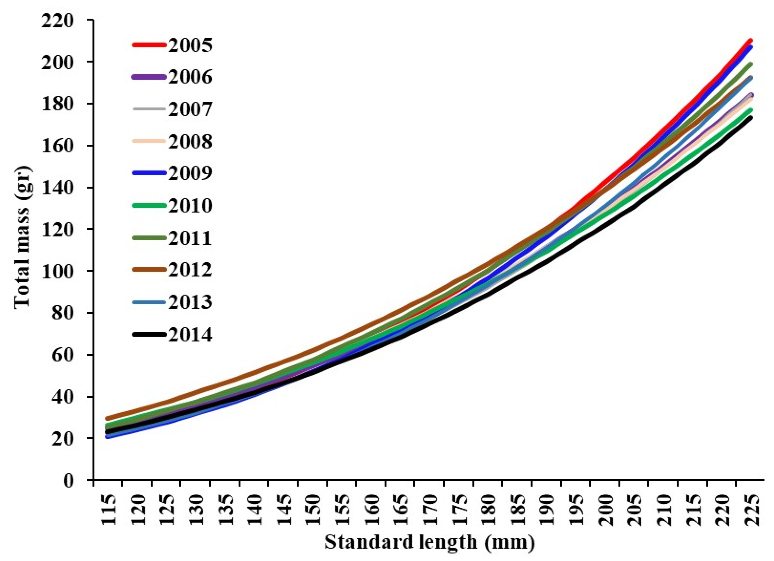
3.6. Annual Growth (2005–2014)

The VBM parameters per year of temperate S. sagax stock are shown in

Table 9. Annual average values and 95% confidence intervals (CI; α = 0.05) of the parameters t₀, k, L_∞, and phi-prima (φ′) obtained from von Bertalanffy growth model for temperate Sardinops sagax stock in the southern California Current System (CCS).

Year	t0 (year)			L∞ (mm)			k (year−1)			φ′
	Lower CI	Mean	Upper CI	Lower CI	Mean	Upper CI	Lower CI	Mean	Upper CI
2005	−2.18	−2.16	−2.13	198.7	199.2	199.7	0.300	0.301	0.302	2.13
2006	−1.17	−1.15	−1.13	188.7	189.2	189.6	0.681	0.687	0.693	2.39
2007	−2.36	−2.33	−2.30	189.6	190.1	190.6	0.398	0.402	0.405	2.16
2008	−0.79	−0.78	−0.76	189.2	189.7	190.2	0.853	0.861	0.870	2.49
2009	−1.53	−1.51	−1.49	196.6	197.0	197.5	0.507	0.511	0.514	2.30
2010	−2.47	−2.44	−2.42	185.9	186.4	186.8	0.397	0.400	0.403	2.14
2011	−0.76	−0.75	−0.74	189.4	189.7	190.1	0.887	0.894	0.901	2.51
2012	−1.01	−1.00	−0.99	199.2	199.6	200.0	0.676	0.680	0.685	2.43
2013	−0.77	−0.76	−0.74	208.6	209.0	209.5	0.740	0.746	0.752	2.51
2014	−1.29	−1.27	−1.26	210.9	211.3	211.8	0.526	0.529	0.533	2.37

, which reveal interannual variability, where asymptotic length (L_∞) oscillated from 186.4 to 211.0 mm SL with an average of 214.6 mm, the growth coefficient (k) varied from 0.301 to 0.894 year⁻¹ with an average of 0.383, and the age at which length was zero (t₀) was from −2.44 to −0.75 years old. As a growth performance indicator, the phi-prima (φ’) index had values from 2.13 to 2.51 with an average of 2.25 (Table 9).

3.7. Relationship between Individual Growth and Environmental Conditions

The variation among φ′ anomaly and average annual values of PDO, ONI, and UI are shown in Figure 9. The behavior between φ′ anomaly and PDO and ONI indicated that there is an inverse behavior with both indices, i.e., the highest values of φ′ coincided with the lowest values of ONI and PDO. In contrast, the variation between φ′ anomaly and UI showed a similar trend. However, in all cases, the linear relationships were not statistically significant (p > 0.05).

4. Discussion

The study, evaluation, and appropriate management of Pacific sardine (S. sagax) in the southern part of the California Current will depend on a precise differentiation of the stocks that are distributed in this region and that are supposed to have certain synchrony in their migratory behavior, which translates into suitably differentiated entities [9,61]. A method to differentiate landings from Pacific sardine stocks using concomitant measurements of sea surface temperature (SST) was proposed by Félix-Uraga et al. (2004, 2005) [7,8]. Later, Demer and Zwolinski [10] corroborated and refined the method using regional indices of optimal potential habitat for the northern population and indices based on SST associated with the potential habitat. They found that landings of the temperate stock in Ensenada, BC, Mexico, on average were 63–72%, while 32–36% of the stock was landed in San Pedro, California, USA. In our work, of total catch landings, an approximate average of 66% were from the temperate stock, 13% corresponded to the cold stock (<17 °C), and 21% corresponded to the warm stock (>22 °C); the latter landed in Magdalena Bay, BCS, Mexico. This method of differentiating stocks is considered adequate [10], since it allows for the improvement of the definition of size structure, ages, and length–weight relationships, as well as of the subsequent estimations of biomass of the temperate stock, recruitment, and mortality. Notwithstanding the above, we must emphasize that the method is not exempt from errors in the allocation of stocks, particularly during periods of habitat transition, in which finer spatial and/or temporal scales could be used [10].

The size structure observed for the temperate S. sagax stock was integrated into 12 age groups (0.5–6.0). However, the predominant sardines were from age groups 1 to 3, which accounted for 82% of the catches. The results agree with the age structure described for Bahía Magdalena (0–5) [24,62]. In the northernmost part of the geographical distribution area of S. sagax, older ages (at least 8 years) have been reported, where sardines from 2 to 5 years predominate [5,12,63]. These differences could be explained by the cold stock of S. sagax being distributed in a colder habitat with a different environmental dynamic than that observed along the coasts of the Baja California peninsula, which allows sardines from the cold stock to reach larger sizes and ages [64,65].

The allometry body mass results for the temperate S. sagax stock showed hyper-allometric growth (b = 3.155), indicating that S. sagax grows more in volume (mass) than in length [41]. The allometry coefficient average values estimated were found in agreement with those reported for this species by García-Alberto [66], who estimated b values of 3.034, 3.130, and 3.159 for Bahía Magdalena, Ensenada, and San Pedro, respectively. Nonetheless, the b values estimated in this study showed notable interannual fluctuations (from b = 2.790 to 3.493), which is why interannual changes took place from hyper- to hypo-allometric growth type. These values are deemed acceptable considering that, in wide distribution species, as is the case of S. sagax, they may be found in heterogeneous habitats, consequently having a wide variation range in the allometry parameter [67]. According to the b values estimated by García-Alberto [66] with an ascending tendency of b concerning latitude, this pattern may be explained with Bergmann’s Rule, considering that the highest b values infer a better condition and suggest that body mass increases toward greater latitudes and/or lower temperatures [68], as pointed out for the epipelagic species Peprilus medius [43]. Therefore, because S. sagax is a highly migratory organism, its population may be affected along its displacement for different factors that have a bearing on its condition, such as thermoregulation, productivity (food availability), age, or maturity stage [66,68].

The temperate stock, during winter and summer, has a wide distribution from Bahia Magdalena to Ensenada, but catches of this stock are higher in Bahia Magdalena during winter, while, in Ensenada, they are higher in summer. However, in spring, when the stock has its southernmost distribution, catches are higher in Bahia Magdalena, whereas, in autumn, when the stock has its northernmost distribution, catches are higher in Ensenada. This behavior of the catches is related to the migratory behavior of the stock, which in turn is closely related to the seasonal behavior of both the SST and the upwelling [61]. These differences in the environment inhabited by the temperate stock could cause the sardines caught in the Ensenada, Isla Cedros, and Bahía Magdalena areas to present changes in weight for a given size or in reproductive behavior in such a way that this would be reflected in the growth of sardines. In other words, perhaps in one area, a sardine grows more in length, while, in another area, it grows more in weight or reproduces more.

Estimating fish growth is critical to understanding life history and conducting fishery assessments [17,52,53,69]. It is very important when estimating individual fish growth that each size and age class of fish is sufficiently sampled to build models that accurately reflect biological growth patterns, particularly for commercially exploited species in which the largest, older individuals may be less abundant and smaller individuals may not yet be recruited to the fishery. Therefore, it should be considered that it is highly likely that these age and size groups are not very well represented in our samples and that the results may not adequately represent the individual growth of the fish stock. Therefore, the possible bias that samples with these characteristics could have in the estimation of the parameters of the growth model must be evaluated in such a way that it can be incorporated into the estimation process. In that context, this study addressed that concern using a simulation exercise [52,53] to understand how the characteristics of our original data affected the results obtained. Therefore, with the raw data, the LM model had the highest WAIC (~35%), while the VBM model had a WAIC of only ~18%. However, when the bolstered raw data were fitted, the VBM model had the highest WAIC (~61%), while the LM model had null plausibility. The simulation of an ideal sampling scenario in which each age class was equally represented revealed that the inadequate representation of the young and very old age groups could change the result regarding which model feasibly describes the growth of the Pacific sardine in the south of the CCS. Consequently, we found that the von Bertalanffy growth model suitably described the growth pattern of the Pacific sardine, which appears to be more robust against biased data. This finding agrees with a similar study for the Gulf of California specie where the greatest plausibility was for the VBM [18].

Our results allow us to consider the use of the VBM model acceptable to compare with other studies performed for this species [12,15,21,22,23,70,71], as well as its usefulness as an input parameter in future abundance and population dynamics assessment of the temperate S. sagax stock. This model has been useful to represent fish growth, mainly for species of commercial interest. The growth parameters may differ within the same population, i.e., growth parameters for this species may have different values depending on their distribution area and ecosystem dynamics [8,12,14,15,31,72,73,74,75]. Moreover, successive cohorts may also grow differently according to habitat conditions and affect growth parameter values [12].

The AIC approach, commonly used in growth studies, balances model complexity (number of parameters) and goodness of fit (likelihood), but does not necessarily provide the most unbiased parameter estimates. Fixing model parameters may seem like an appealing approach, particularly when faced with few data, and one degree of freedom can be saved in the estimation of parameters. However, in the case of the VBM-2, we show how fixing $t_0$ results in a substantial risk of estimating a biased growth parameter, outweighing any benefits of this approach. VBM-2 increases the bias in growth parameters estimates and, in this case, the highest bias was recorded for parameter $k$ (52.11%), which can further affect its use as a proxy in life-history estimation and stock assessments. The finding in this study is consistent with that reported by Pardo et al. [56]. Given that the $t_0$ and the $L_0$ parameterizations are mathematically equivalent, fixing them to a specified value would result in the same mathematical constraints and, hence, similar effects on model performance to those highlighted in our study [56,76].

The parameters obtained by VBM-3 revealed lower CV and biases than estimated by VBM-2, where the mean values estimated by VBM-3 were close to the parameters estimated via the objective maximum likelihood function. These results reveal that the CI for the estimated parameters by VBM-3 had more accuracy. However, testing the performance of this approach under uncertain $t_0$ parameter values should be the focus of further investigation.

The growth performance index (φ′) proposed by Pauly and Munro [60] was a useful way to prove if the growth parameters ($L_{\infty }$, y, $k$) for the same species generated from a new set of data were adequate. De Anda-Montañez et al. [15] estimated index φ′ values for the Gulf of California species from 2.3 to 2.7 and the United States and Canada with very similar values from 2.4 to 2.7. In Bahía Magdalena, Álvarez-Trasviña [72] found values oscillating from 2.0 to 2.7, which is why those φ′ values estimated in this study (2.1 to 2.5) for the temperate S. sagax stock with the VBM model parameters may be considered adequate. Although φ′ values were similar among the different distribution areas, in the northern latitudes (USA and Canada), their variation interval was lower (cold stock) than that in the southern CCS (temperate stock). This result can be explained by the variations in environmental conditions being more heterogeneous south of the CCS than in the northern part [77]. Fish may show changes and a greater variation in their growth patterns due to changes in their biotic and abiotic relationships [78,79], which may result in a greater growth performance variation in the temperate stock organisms that inhabit a more heterogeneous environment than their northern congeners. In this sense, interannual variability was also observed in the growth parameters and φ′values found for temperate S. sagax stock. The apparent inverse relationship observed between φ’ and the ONI or the PDO and the apparent positive relationship between UI and φ′ would indicate that, in the years in which there were warm water conditions (e.g., El Niño), the values of φ′would possibly tend to be the lowest, while the opposite could occur with relatively cold conditions (e.g., La Niña). Therefore, it is possible that, during warm water conditions, the Pacific sardine may grow less (smaller and/or thinner) due to a decrease in quality available preys, as the subtropical species, which tend to be smaller and less nutritious, could be more abundant during warm conditions [35], while the opposite would occur under temperate or relatively cold conditions. In this context, a possible mechanism that could explain the behavior observed in growth and allometry could be a bottom-up process. This opens a way of working to explore, in the near future, the relationship between growth variation and temperature, incorporating more years with growth data and using different environmental indices, which would reflect environmental variability in interannual and decadal scales. It is worth mentioning that interannual variation could also be a consequence of incorporating new cohorts in the population since recruiting changes have been pointed out as a way of incorporating annual variability in individual growth [12,80]. Lastly, it is important to point out that growth can also be approached using random or mixed effects models (random and fixed), through which the effects that different intrinsic and extrinsic covariates have on the estimation of growth and its variability have been explored [79,81,82,83,84,85,86]. On the other hand, it has been noted that integrated mixed-effects models could reduce bias in growth model parameters versus non-integrated models [87], but that this line of research has not yet fully explored the performance of integrated mixed-effects models to simultaneously estimate unknown ages, growth model parameters, and derived variables. In this context, for this species, there is an open route in which the growth of the different Pacific sardine stocks that inhabit the California Current and the Gulf of California can be explored.

5. Conclusions

Overall, this article provided information on individual growth and allometry not currently available for the entire temperate stock of the Pacific sardine (S. sagax), which will help us further our understanding of its biology. The sample distribution has an important influence on the growth model selection; as pointed out in other works, the data used must be carefully examined to avoid biases in data influencing the selection of a growth model that is not biologically realistic. In this work, the von Bertalanffy growth model suitably represented the biological reality of S. sagax, seemed to be more robust against biased data and was statistically comparable with the contrasted models. The comparison between the von Bertalanffy model with three and two parameters (t₀ fixed) indicated that the two-parameter model estimated more biased values and with a higher CV than the three-parameter model, mainly affecting parameter k. Interannual variability was observed in growth parameters for the temperate stock of S. sagax, coupled with an apparent relationship between φ′ and some environmental indices (ONI, PDO, and UI).

References

1. Wolf, P. Recovery of the Pacific sardine and the California sardine fishery. Calif. Coop. Ocean. Fish. Investig. Rep. 1992, 33, 76–86. [Google Scholar]
2. Deriso, R.B.; Barnes, J.T.; Jacobson, L.D.; Arenas, P.R. Catch-at-age analysis for Pacific sardine (Sardinops sagax), 1983–1995. Calif. Coop. Ocean. Fish. Investig. Rep. 1996, 37, 175–187. [Google Scholar]
3. Smith, P.E. Biological effects of ocean variability: Time and space scales of biological response. Rapp. Proces Verbaux Reun. Cons. Int. Explor. Mer 1978, 173, 117–127. [Google Scholar]
4. Parrish, R.H.; Serra, R.; Grant, W.S. The monotypic sardines, Sardina and Sardinops: Their taxonomy, distribution, stock structure, and zoogeography. Can. J. Fish. Aquat. Sci. 1989, 46, 2019–2036. [Google Scholar] [CrossRef]
5. Emmett, R.L.; Brodeur, R.D.; Miller, T.W.; Pool, S.S.; Bentley, P.J.; Krutzikowsky, G.K.; McCrae, J. Pacific Sardine (Sardinops sagax) Abundance, Distribution, and Ecological Relationships in the Pacific Northwest. Calif. Coop. Ocean. Fish. Investig. Rep. 2005, 46, 122–143. [Google Scholar]
6. Kramer, D.; Smith, P.E. Seasonal and geographic characteristics of fishery resources. California current region VII. Pacific Sardine. Commer. Fish. Rev. 1971, 33, 7–11. [Google Scholar]
7. Félix-Uraga, R.; Gómez-Muñoz, V.M.; Quiñonez-Velázquez, C.; Melo-Barrera, F.N.; García-Franco, W. On the Existence of Pacific Sardine Groups off the West Coast of Baja California and Southern California. Calif. Coop. Ocean. Fish. Investig. Rep. 2004, 45, 146–151. [Google Scholar]
8. Félix-Uraga, R.; Gómez-Muñoz, V.M.; Quiñonez-Velázquez, C.; Melo-Barrera, F.N.; Hill, K.; García-Franco, W. Pacific Sardine (Sardinops sagax) Stock Discrimination off the West Coast of Baja California and Southern California Using Otolith Morphometry. Calif. Coop. Ocean. Fish. Investig. Rep. 2005, 46, 113–121. [Google Scholar]
9. Smith, P.E. A History of Proposals for Subpopulation Structure in the Pacific Sardine (Sardinops sagax) Population off Western North America. Calif. Coop. Ocean. Fish. Investig. Rep. 2005, 46, 75–82. [Google Scholar]
10. Demer, D.A.; Zwolinski, J.P. Corroboration and refinement of a method for differentiating landings from two stocks of Pacific sardine (Sardinops sagax) in the California Current. ICES J. Mar. Sci. 2014, 71, 328–335. [Google Scholar] [CrossRef]
11. Demer, D.A.; Zwolinski, J.P. Optimizing fishing quotas to meet target fishing fractions of an internationally exploited stock of Pacific Sardine. North Am. J. Fish. Manag. 2014, 34, 1119–1130. [Google Scholar] [CrossRef]
12. Dorval, E.; McDaniel, J.D.; Macewicz, B.J.; Porzio, D.L. Changes in growth and maturation parameters of Pacific sardine Sardinops sagax collected off California during a period of stock recovery from 1994 to 2010. J. Fish Biol. 2015, 87, 286–310. [Google Scholar] [CrossRef]
13. DOF. NORMA Oficial Mexicana NOM-003-SAG/PESC-2018, Para Regular el Aprovechamiento de las Especies de Peces Pelágicos Menores con Embarcaciones de Cerco, en Aguas de Jurisdicción Federal del Océano Pacífico, Incluyendo el Golfo de California, Ciudad de México. Secretaria de Gobernación. 2019. Available online: https://www.dof.gob.mx/normasOficiales/7610/sader11_C/sader11_C.html (accessed on 12 March 2019).
14. Checkley, D.M., Jr.; Asch, R.G.; Rykaczewski, R.R. Climate, anchovy, and sardine. Annu. Rev. Mar. Sci. 2017, 9, 469–493. [Google Scholar] [CrossRef]
15. De Anda-Montañez, A.; Arreguín-Sánchez, F.; Martínez-Aguilar, S. Length based growth estimates for pacific sardine (Sardinops sagax) in the Gulf of California, Mexico. Calif. Coop. Ocean. Fish. Investig. Rep. 1999, 40, 179–183. [Google Scholar]
16. Mercier, L.; Panfili, J.; Paillon, C.; N’diaye, A.; Mouillot, D.; Darnaude, A.M. Otolith reading and multi-model inference for improved estimation of age and growth in the gilthead seabream Sparus aurata (L.). Estuar. Coast. Shelf Sci. 2011, 92, 534–545. [Google Scholar] [CrossRef]
17. Lorenzen, K. Toward a new paradigm for growth modeling in fisheries stock assessments: Embracing plasticity and its consequences. Fish. Res. 2016, 180, 4–22. [Google Scholar] [CrossRef]
18. Nevárez-Martínez, M.O.; Arzola-Sotelo, E.A.; López-Martínez, J.; Santos-Molina, J.P.; Martínez-Zavala, M.A. Modeling Growth of the Pacific Sardine Sardinops Caeruleus in the Gulf of California, Mexico, Using the Multimodel Inference Approach. Calif. Coop. Ocean. Fish. Investig. Rep. 2019, 60, 1–13. [Google Scholar]
19. Beddington, J.R.; Kirkwood, G.P. The estimation of potential yield and stock status using life-history parameters. Philos. Trans. R. Soc. B 2005, 360, 163–170. [Google Scholar] [CrossRef]
20. Haddon, M. Modeling and Quantitative Methods in Fisheries, 2nd ed.; Chapman and Hall/CRC: New York, NY, USA, 2011. [Google Scholar] [CrossRef]
21. Alvarado-Castillo, R.M.; Félix-Uraga, R. Edad y crecimiento de la sardina Monterrey Sardinops caeruleus (Pisces: Clupeidae) en Isla de Cedros, Baja California, México, durante 1985 y 1986. Bol. Investig. Mar. Costeras 1996, 25, 77–86. [Google Scholar] [CrossRef]
22. Cisneros-Mata, M.A.; Estrada, J.; Montemayor, G. Growth, mortality and recruitment of exploited small pelagic fishes in the Gulf of California. Fishbyte 1990, 8, 15–17. [Google Scholar]
23. Quiñonez-Velázquez, C.; Alvarado-Castillo, R.; Félix-Uraga, R. Relación entre el crecimiento individual y la abundancia de la población de la sardina del Pacífico Sardinops Caeruleus (Pisces: Clupeidae) (Girard 1856) en Isla de Cedros, Baja California, México. Rev. Biol. Mar. Oceanogr. 2002, 37, 1–8. [Google Scholar] [CrossRef]
24. Félix-Uraga, R. Dinámica Poblacional de la Sardina del Pacífico Sardinops sagax (Jenyns 1842) (Cupleiformes: Clupeidae), en la Costa Oeste de la Península de Baja California y el sur de California. Ph.D. Thesis, CICIMAR, La Paz, México, 2006; 86p. [Google Scholar]
25. Katsanevakis, S. Modelling fish growth: Model selection, multi-model inference and model selection uncertainty. Fish. Res. 2006, 81, 229–235. [Google Scholar] [CrossRef]
26. Katsanevakis, S.; Maravelias, C.D. Modelling fish growth: Multi-model inference as a better alternative to a priori using von Bertalanffy equation. Fish Fish. 2008, 9, 178–187. [Google Scholar] [CrossRef]
27. Ricker, W.E. Computation and interpretation of biological statistics of fish populations. Bull. Fish. Res. Board Can. 1975, 191, 382. [Google Scholar]
28. Schnute, J. A versatile growth model with statistically stable parameters. Can. J. Fish. Aquat. Sci. 1981, 38, 1128–1140. [Google Scholar] [CrossRef]
29. Schnute, J.T.; Richards, L.J. A unified approach to the analysis of fish growth, maturity, and survivorship data. Can. J. Fish. Aquat. Sci. 1990, 47, 24–40. [Google Scholar] [CrossRef]
30. Burnham, K.P.; Anderson, D.R. Model Selection and Multimodel Inference: A Practical Information-Theoretic Approach; Springer: New York, NY, USA, 2002. [Google Scholar] [CrossRef]
31. Félix-Uraga, R. Crecimiento de Sardinops caeruleus en Bahía Magdalena, México. Investig. Mar. 1990, 5, 27–31. [Google Scholar]
32. Durazo, R.; Baumgartner, T.R. Evolution of oceanographic conditions off Baja California: 1997–1999. Prog. Oceanogr. 2002, 54, 7–31. [Google Scholar] [CrossRef]
33. Espinosa-Carreon, T.L.; Strub, P.T.; Beier, E.; Ocampo-Torres, F.; Gaxiola-Castro, G. Seasonal and interannual variability of satellite-derived chlorophyll pigment, surface height, and temperature off Baja California. J. Geophys. Res. 2004, 109, C03039. [Google Scholar] [CrossRef]
34. Durazo, R. Climate and upper ocean variability off Baja California, Mexico: 1997–2008. Prog. Oceanogr. 2009, 83, 361–368. [Google Scholar] [CrossRef]
35. Cavole, L.M.; Demko, A.M.; Diner, R.E.; Giddings, A.; Koester, I.; Pagniello, C.M.L.S.; Paulsen, M.L.; Ramirez-Valdez, A.; Schwenck, S.M.; Yen, N.K.; et al. Biological impacts of the 2013–2015 warm-water anomaly in the Northeast Pacific: Winners, losers, and the future. Oceanography 2016, 29, 273–285. [Google Scholar] [CrossRef] [Green Version]
36. Durazo, R.; Castro, R.; Miranda, L.E.; Delgadillo-Hinojosa, F.; Mejía-Trejo, A. Anomalous hydrographic conditions off the northwestern coast of the Baja California Peninsula during 2013–2016. Cienc. Mar. 2017, 43, 81–92. [Google Scholar] [CrossRef]
37. Nevárez-Martínez, M.O.; Cisneros-Mata, M.A.; Montemayor-López, G.; Santos-Molina, P. Estructura por edad, y crecimiento de la sardina monterrey (Sardinops sagax caeruleus) del Golfo de California, México: Temporada de pesca 1990/91. Cienc. Pesq. 1996, 13, 30–36. [Google Scholar]
38. Yaremko, M. Age Determination in Pacific Sardine, Sardinops sagax; NOAA Technical Memorandum; NOAA-TM-NMFS-SWFSC-223; Southwest Fisheries Science Center: San Diego, CA, USA, 1996; 33p. [Google Scholar]
39. Beamish, R.J.; Fournier, D.A. A method for comparing the precision of a set of age determination. Can. J. Fish. Aquat. Sci. 1981, 38, 982–983. [Google Scholar] [CrossRef]
40. Chang, W.Y.B. A statistical method for evaluating the reproducibility of age determination. Can. J. Fish. Aquat. Sci. 1982, 39, 1208–1210. [Google Scholar] [CrossRef]
41. Froese, R. Cube law, condition factor and weight-length relationships: History, meta-analysis and recommendations. J. Appl. Ichthyol. 2006, 22, 241–253. [Google Scholar] [CrossRef]
42. Sokal, R.R.; Rohlf, F.J. Introduction of Biostatistics, 2nd ed.; Dover Publications, Inc.: New York, NY, USA, 2009. [Google Scholar]
43. Maldonado-Amparo, M.A.; Sanchez-Cardenas, R.; Salcido-Guevara, L.A.; Valdez-Pineda, M.C.; Ramirez-Perez, J.S.; Arzola-González, J.F.; Moreno-Sánchez, X.G.; Marin-Enriquez, E. Length-weight relationship and condition factor of butterfish Peprilus medius (Peters, 1869) in the southeast Gulf of California. Calif. Fish Game 2019, 105, 39–47. [Google Scholar]
44. Von Bertalanffy, L. A quantitative theory of organic growth (inquiries on growth laws II). Hum. Biol. 1938, 10, 181–213. [Google Scholar]
45. Gompertz, B. On the nature of the function expressive of the law of human mortality, and on a new mode of determining the value of life contingencies. Philos. Trans. R. Soc. Lond. 1825, 115, 513–583. [Google Scholar]
46. Neter, J.; Kutner, M.H.; Nachtsheim, J.; Wasserman, W. Applied Linear Statistical Models; McGraw-Hill: New York, NY, USA, 1996; 1408p. [Google Scholar]
47. Venzon, D.J.; Moolgavkor, S.H. A Method for computing profile-likelihood based confidence intervals. J. R. Stat. Society. Ser. C Appl. Stat. 1988, 37, 87–94. [Google Scholar] [CrossRef]
48. Hilborn, R.; Mangel, M. The Ecological Detective. Confronting Models with Data; Princeton University Press: Princeton, NJ, USA, 1997. [Google Scholar]
49. Polacheck, T.; Hilborn, R.; Punt, A.E. Fitting surplus production models: Comparing methods and measuring uncertainty. Can. J. Fish. Aquat. Sci. 1993, 50, 2597–2607. [Google Scholar] [CrossRef]
50. Zar, J.H. Biostatistical Analysis; Prentice-Hall: Englewood Cliffs, NJ, USA, 1999; 633p. [Google Scholar]
51. Pawitan, Y. In All Likelihood: Statistical Modeling and Inference Using Likelihood; Oxford University Press: Oxford, UK, 2001; 528p. [Google Scholar]
52. Bolser, D.G.; Grüss, A.; Lopez, M.A.; Reed, E.M.; Mascareño-Osorio, I.; Erisman, B.E. The influence of sample distribution on growth model output for a highly-exploited marine fish, the Gulf Corvina (Cynoscion othonopterus). PeerJ 2018, 6, e5582. [Google Scholar] [CrossRef]
53. Scherrer, S.R.; Kobayashi, D.R.; Weng, K.C.; Okamoto, H.Y.; Oishi, F.G.; Franklin, E.C. Estimation of growth parameters integrating tag-recapture, length-frequency, and direct aging data using likelihood and Bayesian methods for the tropical deepwater snapper Pristipomoides filamentosus in Hawaii. Fish. Res. 2021, 233, 105753. [Google Scholar] [CrossRef]
54. Goodyear, C.P. Modeling growth: Consequences from selecting samples by size. Trans. Am. Fish. Soc. 2019, 148, 528–551. [Google Scholar] [CrossRef]
55. Kapur, M.; Haltuch, M.; Connors, B.; Rogers, L.; Berger, A.; Koontz, E.; Cope, J.; Echave, K.; Fenske, K.; Hanselman, D.; et al. Oceanographic features delineate growth zonation in Northeast Pacific sablefish. Fish. Res. 2020, 222, 105414. [Google Scholar] [CrossRef]
56. Pardo, S.A.; Cooper, A.B.; Dulvy, N.K. Avoiding fishy growth curves. Methods Ecol. Evol. 2013, 4, 353–360. [Google Scholar] [CrossRef]
57. Neer, J.A.; Thompson, B.A.; Carlson, J.K. Age and growth of Carcharhinus leucas in the northern Gulf of Mexico: Incorporating variability in size at birth. J. Fish Biol. 2005, 67, 370–383. [Google Scholar] [CrossRef]
58. Deriso, R.B.; Quinn, B.J., II; Neal, P.R. Catch-age analysis with auxiliary information. Can. J. Fish. Aquat. Sci. 1985, 42, 815–824. [Google Scholar] [CrossRef]
59. Jacobson, L.D.; Lo, N.C.H.; Barnes, J.T. A biomass-based assessment model for northern anchovy, Engraulis mordax. Fish. Bull. 1994, 92, 711–724. [Google Scholar]
60. Pauly, D.; Munro, L. Once more on growth comparison in fish and invertebrates. Fishbyte 1984, 2, 21. [Google Scholar]
61. García-Morales, R.; Shirasago-German, B.; Félix-Uraga, R.; Perez-Lezama, E.L. Conceptual models of Pacific sardine distribution in the California Current System. Curr. Dev. Oceanogr. 2012, 5, 23–47. [Google Scholar]
62. Melo-Barrera, F.N.; Félix-Uraga, R.; Quiñonez-Velázquez, C. Análisis de la pesquería de Sardinops sagax en la costa occidental de Baja California Sur, México, durante 2006–2008. Cienc. Pesq. 2010, 18, 33–46. [Google Scholar]
63. Hill, K.T.; Lo, N.C.H.; Macewicz, B.J.; Crone, P.R.; Félix-Uraga, R. Assessment of the Pacific Sardine Resource in 2010 for U.S. Management in 2011; NOAA Technical. Memorandum; NMFS-SWFSC-469; U.S. Department of Commerce: La Jolla, CA, USA, 2010; 137p.
64. Lo, N.C.H.; Macewicz, B.J.; Griffith, D.A. Migration of Pacific Sardine (Sardinops sagax) off the West Coast of United States in 2003–2005. Bull. Mar. Sci. 2011, 87, 395–412. [Google Scholar] [CrossRef]
65. McDaniel, J.; Piner, K.; Lee, H.H.; Hill, K. Evidence that the Migration of the Northern Subpopulation of Pacific Sardine (Sardinops sagax) off the West Coast of the United States Is Age-Based. PLoS ONE 2016, 11, e0166780. [Google Scholar] [CrossRef]
66. García-Alberto, G. Reproducción de la Sardina del Pacífico Sardinops Sagax (Jenyns, 1842) en la Región sur de la Corriente de California. Master’s Thesis, CICIMAR, La Paz, México, 2010; 77p. [Google Scholar]
67. Costa, M.R.; Araújo, F.G. Length-weight relationship and condition factor of Micropogonias furnieri (Desmarest) (Perciformes, Sciaenidae) in the Sepetiba Bay, Rio de Janeiro, Brazil. Rev. Bras. De Zool. 2003, 20, 685–690. [Google Scholar] [CrossRef]
68. Meiri, S. Bergmann’s rule—What’s in a name? Glob. Ecol. Biogeogr. 2011, 20, 203–207. [Google Scholar] [CrossRef]
69. Miller, T.J.; O’Brien, L.; Fratantoni, P.S. Temporal and environmental variation in growth and maturity and effects on management reference points of Georges Bank Atlantic cod. Can. J. Fish. Aquat. Sci. 2018, 75, 2159–2171. [Google Scholar] [CrossRef]
70. Barnes, J.T.; Foreman, T.J. Recent evidence for the formation of annual growth increments in the otoliths of young Pacific sardines (Sardinops sagax). Calif. Fish Game 1994, 79, 29–35. [Google Scholar]
71. Álvarez-Trasviña, E. Variabilidad en el Crecimiento Individual de la Sardina del Pacífico Sardinops Sagax (Jenyns 1842) y su Relación con el Ambiente en Bahía Magdalena, B.C.S. Master’s Thesis, CICIMAR, La Paz, México, 2012; 45p. [Google Scholar]
72. Holt, S.J. A preliminary comparative study of the growth, maturity and mortality of sardines. In Proceedings of the World Scientific Meeting on the Biology of Sardines and Related Species, Rome, Italy, 14–21 September 1959; FAO: Rome, Italy, 1960; Volume 2, pp. 553–561. [Google Scholar]
73. Beverton, R.J.H. Maturation, growth and mortality of clupeid and engraulid stocks in relation to fishing. Rapp. Procès Verbaux Réunions Cons. Perm. Int. Explor. Mer 1963, 1954, 44–67. [Google Scholar]
74. Méndez-Dasilveira, B. Edad y Crecimiento de Sardinops Sagax Caerulea en el Golfo de California. Bachelor’s Thesis, Facultad de Ciencias, Universidad de Guadalajara, Guadalajara, México, 1987; 91p. [Google Scholar]
75. Jiménez-Rodríguez, J.G. Análisis Comparativo del Crecimiento y la Estructura Poblacional de Sardina Monterrey Sardinops Caruleus (Girard) en el Golfo de California de las Temporadas 1988/1989 y 1989/1990. Bachelor’s Thesis, Escuela de Biología, Universidad Autónoma de Guadalajara, Guadalajara, México, 1991; 60p. [Google Scholar]
76. Cailliet, G.M.; Smith, W.D.; Mollet, H.F.; Goldman, K.J. Age and growth studies of chondrichthyan fishes: The need for consistency in terminology, verification, validation, and growth function fitting. Environ. Biol. Fishes 2006, 77, 211–228. [Google Scholar] [CrossRef]
77. McClatchie, S. Oceanography of the Southern California Current System Relevant to Fisheries. In Regional Fisheries Oceanography of the California Current System; Springer: Dordrecht, The Netherlands, 2014; pp. 13–60. [Google Scholar] [CrossRef]
78. Helfman, G.S.; Collette, B.B.; Facey, D.E.; Bowen, B.W. The Diversity of Fishes, 2nd ed.; Wiley-Blackwell: Hoboken, NJ, USA, 2009. [Google Scholar] [CrossRef]
79. Veron, M.; Duhamel, E.; Bertignac, M.; Pawlowski, L.; Huret, M. Major changes in sardine growth and body condition in the Bay of Biscay between 2003 and 2016: Temporal trends and drivers. Prog. Oceanogr. 2020, 182, 102274. [Google Scholar] [CrossRef]
80. Félix-Uraga, R.; Melo-Barrera, F.N.; Quiñones-Velázquez, C. Parámetros poblacionales de la sardina del Pacífico Sardinops sagax y su contribución a la pesquería de Bahía Magdalena: Enfoques de stocks. In Estudios Ecológicos en Bahía Magdalena; Funes-Rodríguez, R., Gómez-Gutiérrez, J., Palomares-García, R., Eds.; CICIMAR-IPN: La Paz, México, 2007; pp. 221–230. [Google Scholar]
81. Cope, J.M.; Punt, A.E. Admitting Ageing Error When Fitting Growth Curves: An Example Using the Von Bertalanffy Growth Function with Random Effects. Can. J. Fish. Aquat. Sci. 2007, 64, 205–218. [Google Scholar] [CrossRef]
82. Thorson, J.T.; Minte-Vera, C.V. Relative magnitude of cohort, age, and year effects on size at age of exploited marine fishes. Fish. Res. 2016, 180, 45–53. [Google Scholar] [CrossRef]
83. Morrongiello, J.R.; Thresher, R.E. A statistical framework to explore ontogenetic growth variation among individuals and populations: A marine fish example. Ecol. Monogr. 2015, 85, 93–115. [Google Scholar] [CrossRef]
84. Cadigan, N.G.; Campana, S.E. Hierarchical Model-Based Estimation of Population Growth Curves for Redfish (Sebastes mentella and Sebastes fasciatus) off the Eastern Coast of Canada. ICES J. Mar. Sci. 2017, 74, 687–697. [Google Scholar] [CrossRef]
85. Lee, Q.; Punt, A. Extracting a time-varying climate-driven growth index from otoliths for use in stock assessment models. Fish. Res. 2018, 200, 93–103. [Google Scholar] [CrossRef]
86. Dey, R.; Cadigan, N.; Zheng, N. Estimation of the von Bertalanffy Growth Model When Ages Are Measured with Error. J. R. Stat. Soc. Ser. C Appl. Stat. 2019, 68, 1131–1147. [Google Scholar] [CrossRef]
87. Chasco, B.E.; Thorson, J.T.; Heppell, S.S.; Avens, L.; McNeill, J.B.; Bolten, A.B.; Bjorndal, K.A.; Ward, E.J. Integrated mixed-effect growth models for species with incomplete ageing histories: A case study for the loggerhead sea turtle Caretta caretta. Mar. Ecol. Prog. Ser. 2020, 636, 221–234. [Google Scholar] [CrossRef]
Figure 2. Standard length frequency distribution of the temperate Sardinops sagax stock in the southern California Current System (CCS) during the study period (2005–2014).
Fishes 07 00226 g002
Figure 3. (a) Total body mass and standard length (TMSL) relationship for the Sardinops sagax temperate stock in the southern California Current System (CCS); (b) likelihood profiles for parameters a and b obtained for the TMSL relationship.
Fishes 07 00226 g003
Figure 4. Total body mass and standard length (TMSL) relationship per year for the Sardinops sagax temperate stock in the southern California Current System (CCS). Parameters a and b are presented in Table 2.
Fishes 07 00226 g004
Figure 5. Monthly relative frequencies of otoliths with opaque edge (white circle) and hyaline (black circle) for the temperate Sardinops sagax stock in the southern California Current System (CCS) from 2005 to 2014.
Fishes 07 00226 g005
Figure 6. Age (years) frequency distribution of the temperate Sardinops sagax stock in the southern California Current System (CCS) during study period (2005–2014).
Fishes 07 00226 g006
Figure 7. Growth models adjusted to age-at-length data bolstered of the temperate Sardinops sagax stock in the southern California Current System (CCS) during study period (2005–2014).
Fishes 07 00226 g007
Figure 8. Monte Carlo simulation for parameters estimated by the von Bertalanffy Model of the temperate Sardinops sagax stock considering (A) two parameters (t0 fixed) and (B) three parameters.
Fishes 07 00226 g008
Figure 9. Relationship between the growth performance anomalies ( φ ) of the temperate Sardinops sagax stock and environmental indices (PDO, ONI, and UI).
Fishes 07 00226 g009