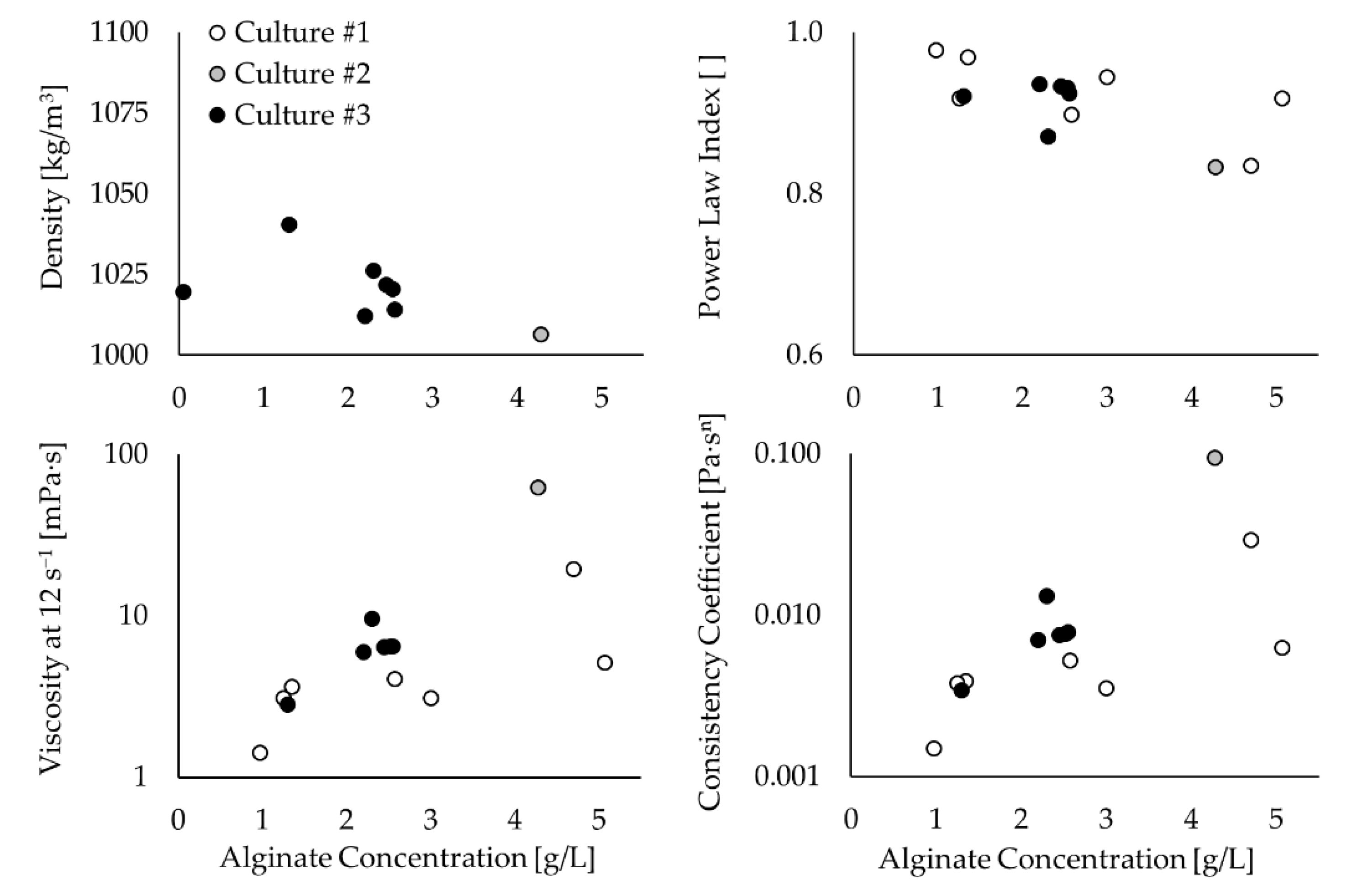
3.1. Fermentation Broth Physical and Rheological Characterization
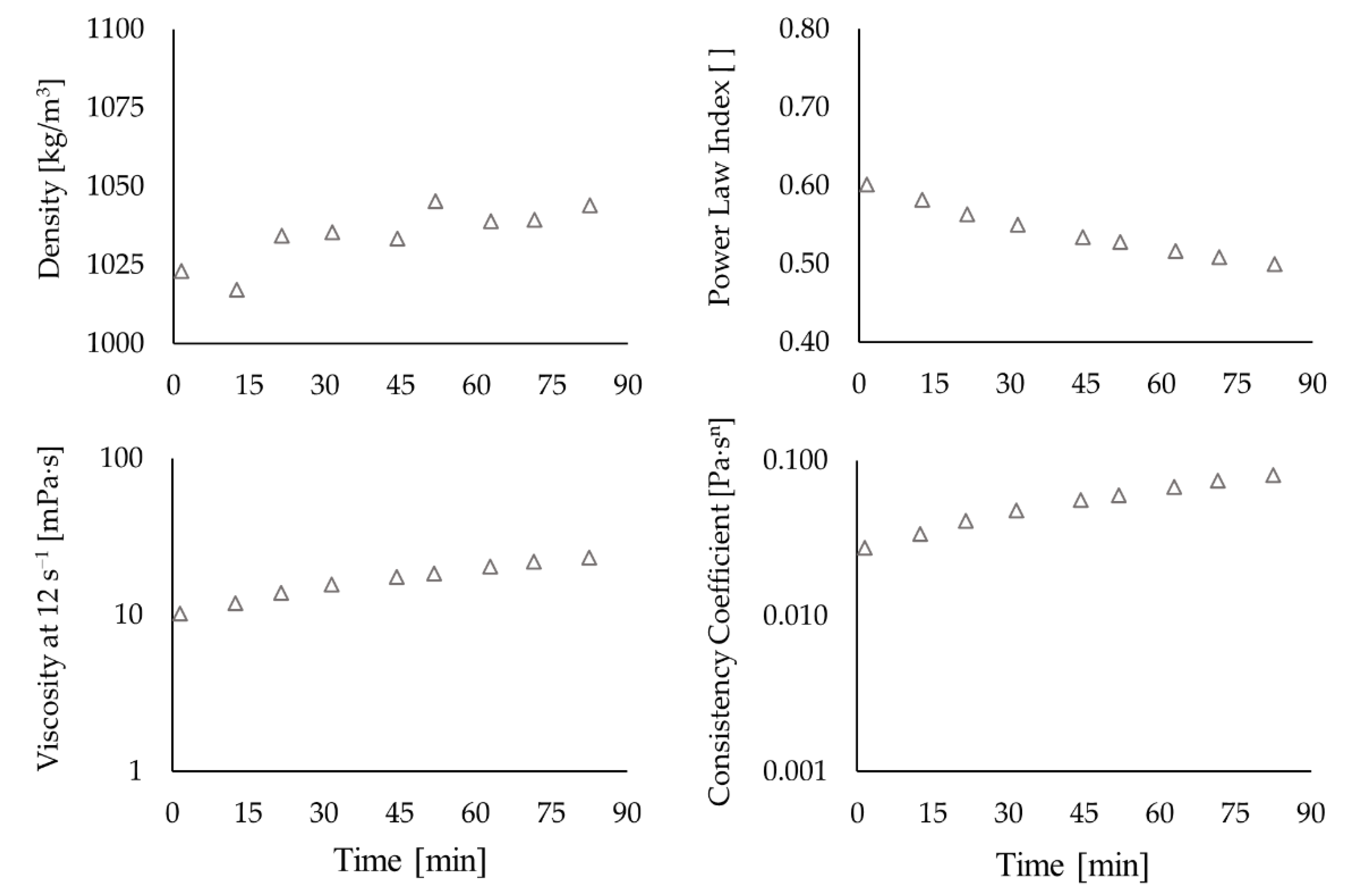
The rheological characterization of the fermentation samples confirmed the non-Newtonian pseudoplastic behaviour of the culture medium because the power-law index decreases below one as the alginate concentration increases (see
Figure 4). Exceptions were found at alginate concentrations below 1 g/L when the culture medium behaves as a Newtonian fluid with a viscosity similar to water. On the other hand, the consistency coefficient shows a trend to increase with the alginate concentration but with very dispersed values. The density also shows scattered values but within a narrow range between 1000 kg/m
3 and 1040 kg/m
3 (see
Figure 4).
The highest viscosity of the culture medium was associated with an alginate concentration of around 4.5 g/L, and varied between 19 and 62 mPa∙s (at 12 s
−1) among the cultures (see
Figure 4). This result is in good agreement with Peña et al. [
2], who reported viscosities between 20 and 420 mPa∙s (at 12 s
−1) for 4 g/L of alginate produced in a 1.0 L system stirred at 300 rpm by three Rushton turbines, under different controlled DOT values.
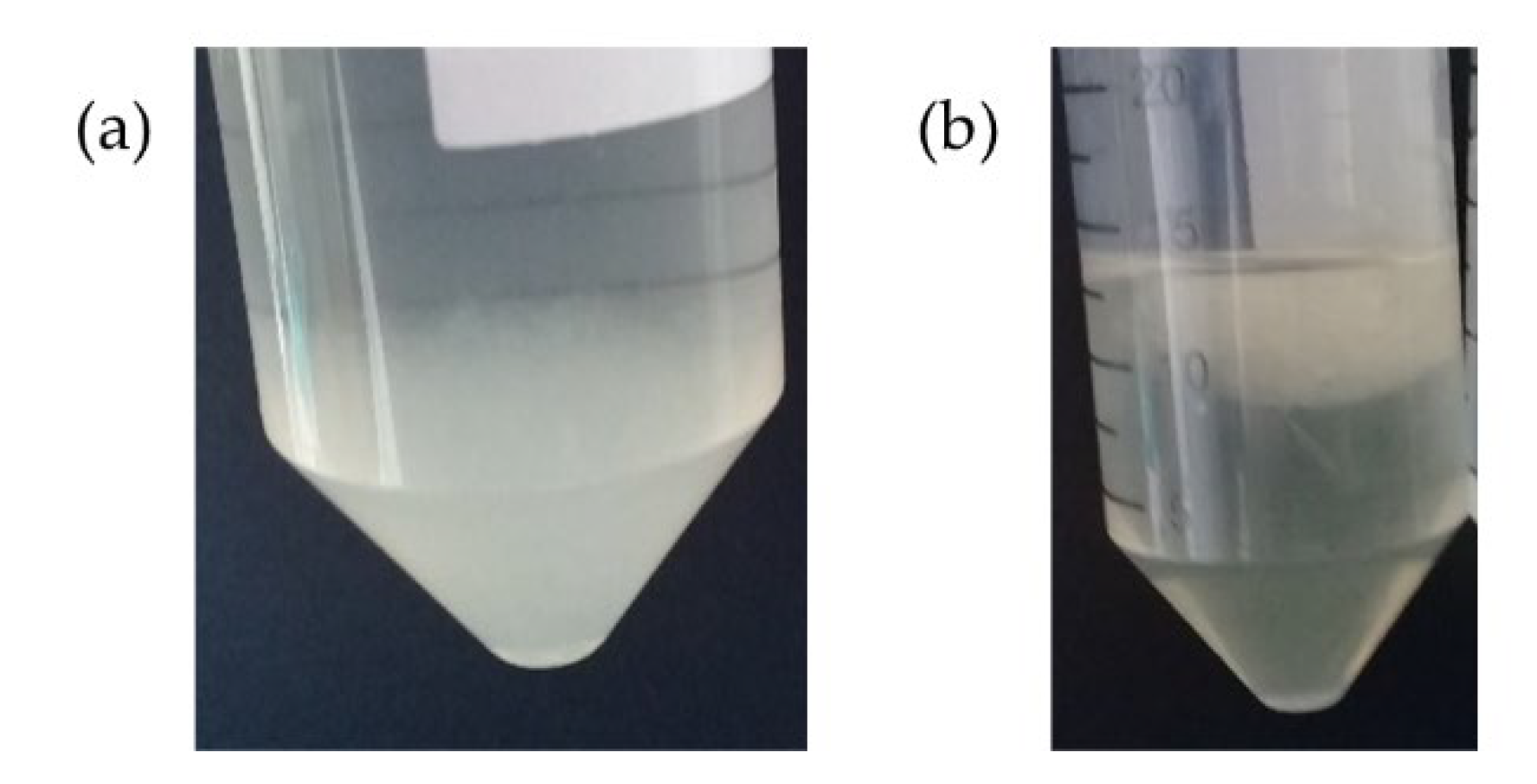
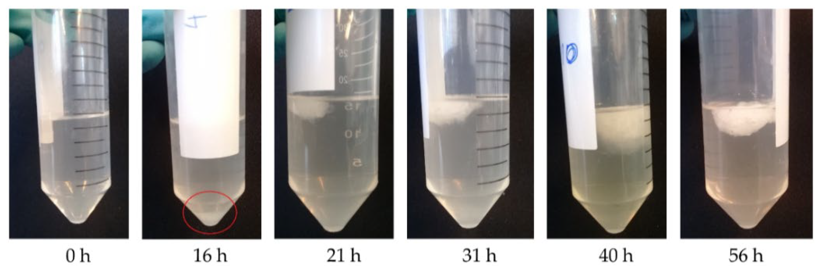
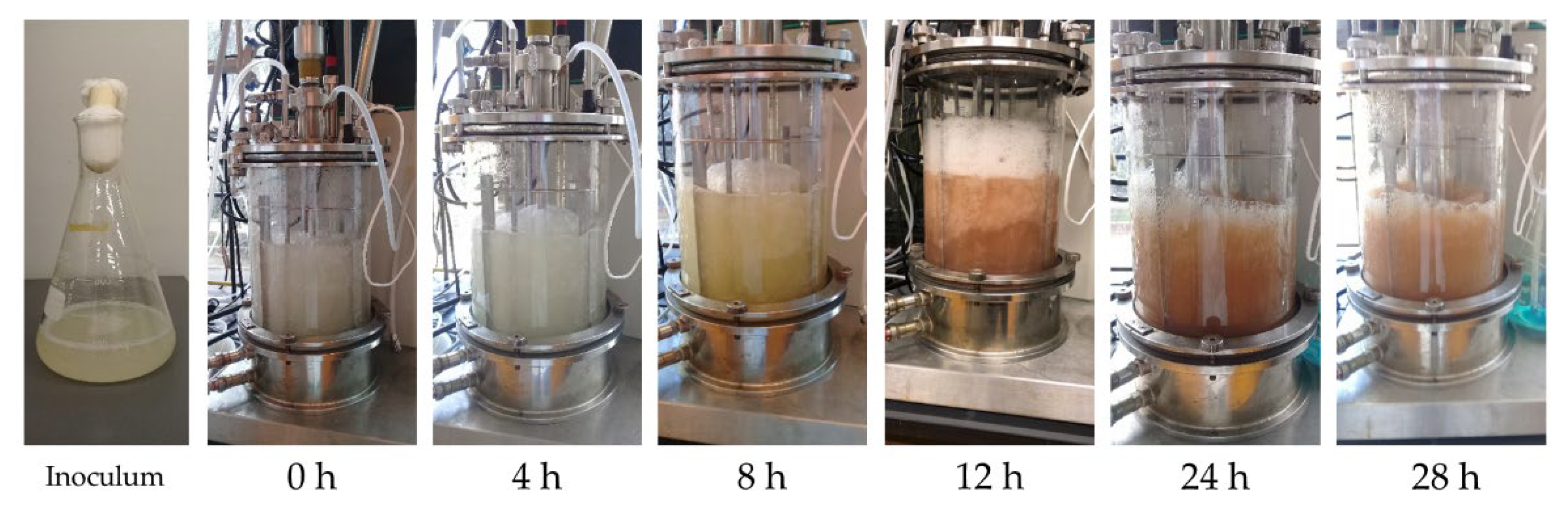
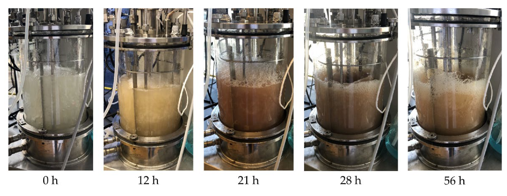
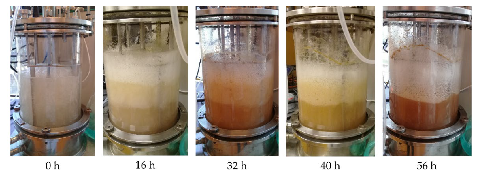
It is important to mention that the sampling from the cultures became more difficult as the alginate concentration increased because the mixing close to the sampler probe became poorer, and, therefore, the sample may not represent adequately other parts of the system. Furthermore, despite the existence of a pH control unit, the pH of the culture medium increased during the fermentations. This may also be due to the mixing problems triggered by the high viscosity of alginate. All these operational difficulties and the complex and inherently variable nature of the microorganisms may cause variations in the process itself. Indeed, the characteristics of the alginate aggregates changed during the process. This was observed after the precipitation and resuspension of alginate from the broth samples. For culture #1, the alginate aggregate of the samples at times 30 and 51 h had a disaggregated and a compact look, respectively, while a compact aspect was observed for most of the re-suspended alginate of culture #2 (see
Appendix E). Furthermore, large variations in the consistency coefficient of the broth samples were registered among the triplicates. Both facts may respond to a variation in the molecular composition of the alginate that can affect its intrinsic viscosity and gelling properties [
29].
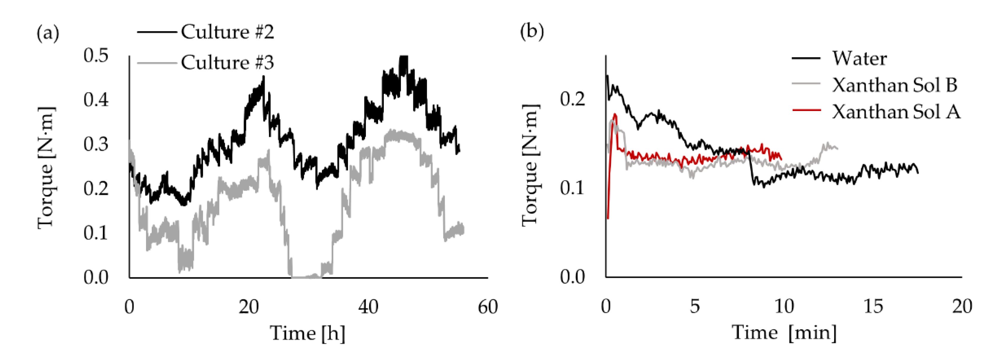
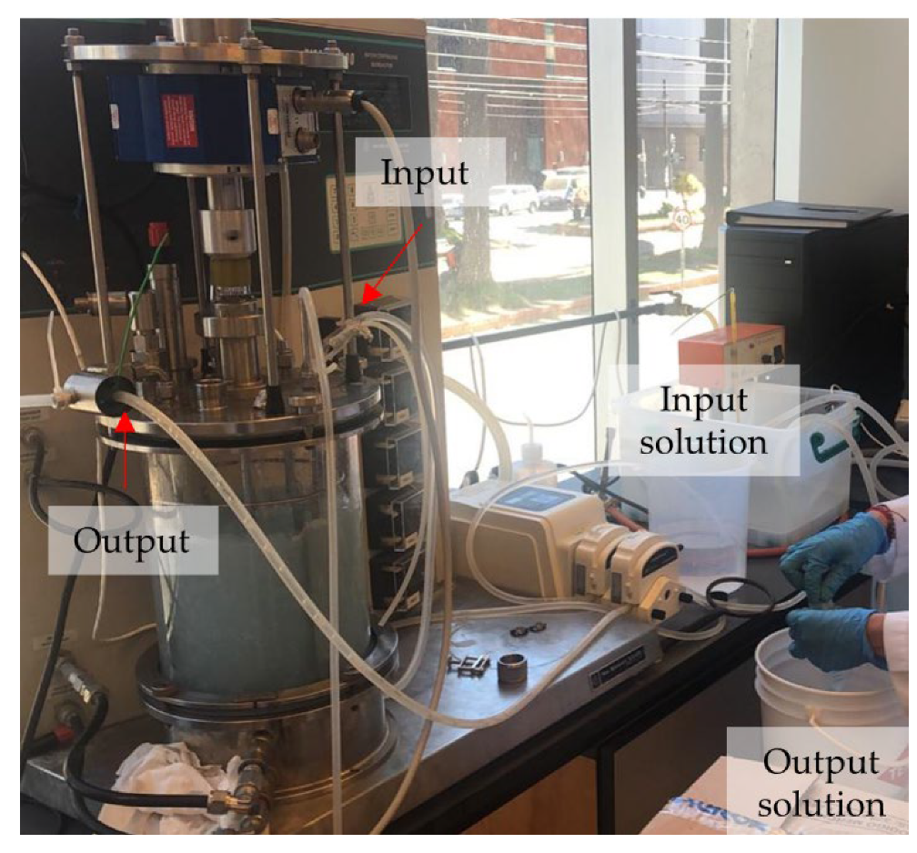
3.2. Experimental Torque Characterization
Due to the broth opacity (see
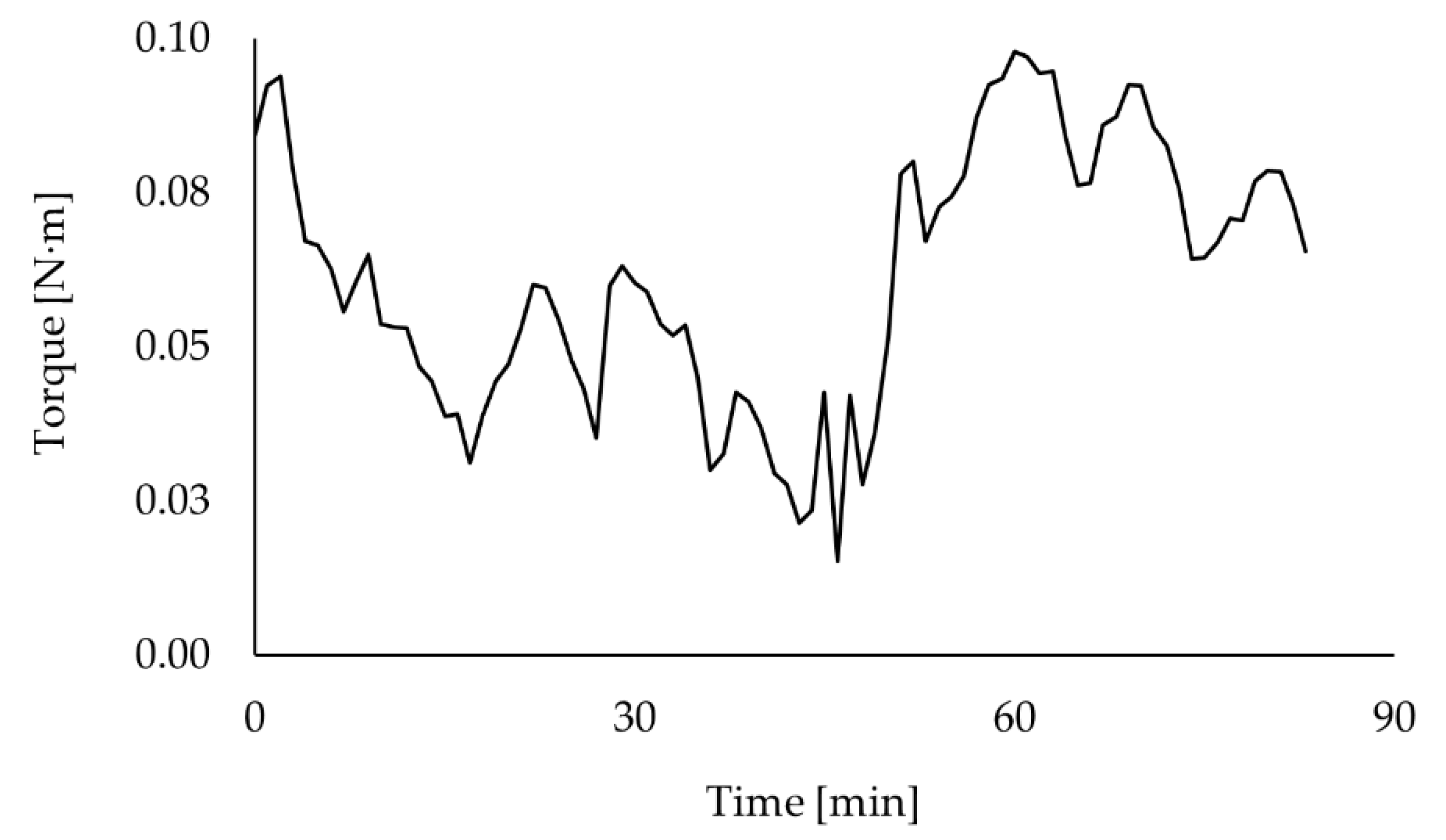
Appendix E), the shaft torque measurement was the most suitable technique that could be used to monitor the fluid dynamics over the fermentation. Unfortunately, the torque data registered during culture #1 had to be discarded due to a technical problem. The torque curve shows similar behaviour for cultures #2 and #3 (see
Figure 5a). The curves are separated by an almost constant gap, except at around hour 30. That bigger gap was caused by an earthquake (6.7 Mww in Chile [
30]) that occurred during culture #3 and affected the performance of the torque meter calibration over a few hours.
Both torque curves have significant small oscillations as part of bigger oscillations. This could be explained by the interaction of different factors, such as mechanical mixing, aeration, and rheological changes. However, due to the complexity of the system, it is difficult to identify how each of these factors contributes to the bioreactor fluid dynamics and, thus, to its torque curve. Therefore, it was necessary to study the abiotic systems to be able to isolate the effect of those factors at different stages of the fermentation process.
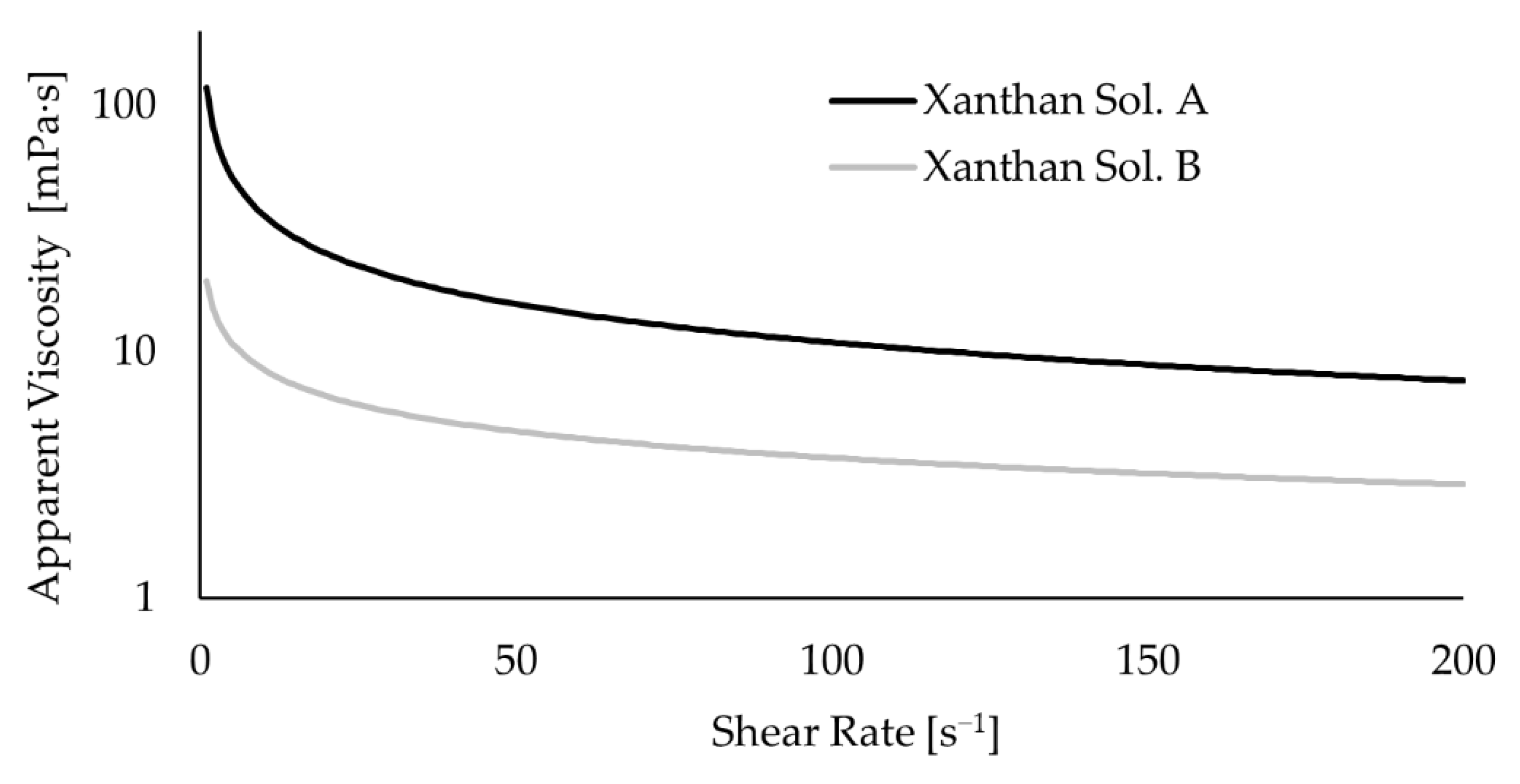
The study of the abiotic systems enabled us to analyze the impact of the mechanical mixing on the torque and how the extent of that impact depends on the rheological characteristics of the fluid (see
Figure 5b). The case with water shows more torque oscillations. It may be explained by the onset of vortical macro-instabilities along the impeller shaft, as discussed in
Section 3.5 which make the initial stabilization of the system more difficult. On average, the system with water had a lower torque than the cases with xanthan solution and, though a slight difference, Xanthan Sol B had a lower torque than Xanthan Sol A (see
Table 4). That is in agreement with the fluid viscosity differences as, under the same operating conditions, a higher torque was obtained for a fluid with a higher viscosity.
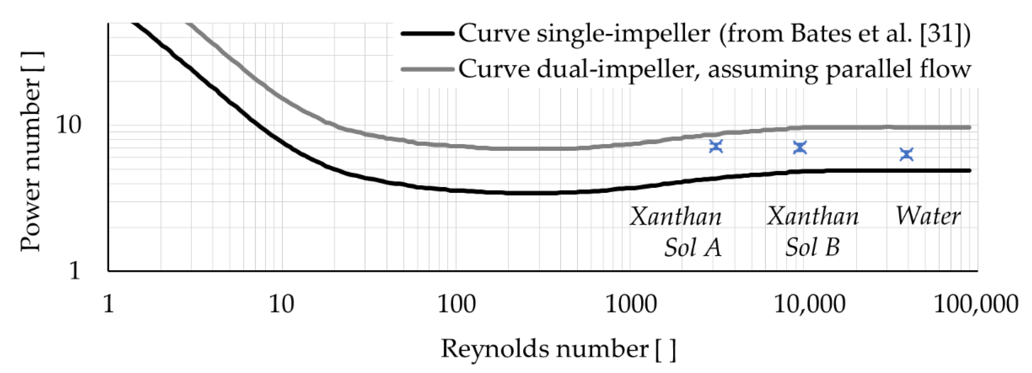
Figure 6 compares the power number experimentally obtained for the abiotic systems versus the one expected for a dual-impellers reactor with a parallel flow (see
Appendix C). The Reynolds number of the abiotic systems is given in
Table 4, while the power number was estimated from the experimental torque based on equations given in
Appendix C. It can be observed that, under the same operating conditions, the system with the highest viscosity (Xanthan Sol A) had a power number more similar to the value expected for dual-impellers with a parallel flow, and the system with the lowest viscosity (water) had a power number more similar to a single-impeller tank, while the other system was in an intermediate situation. Therefore, it is proposed that viscosity had a fundamental role in the flow pattern definition as it determined the level of interaction between the impellers. Particularly, the impeller interaction decreased as the viscosity increased.
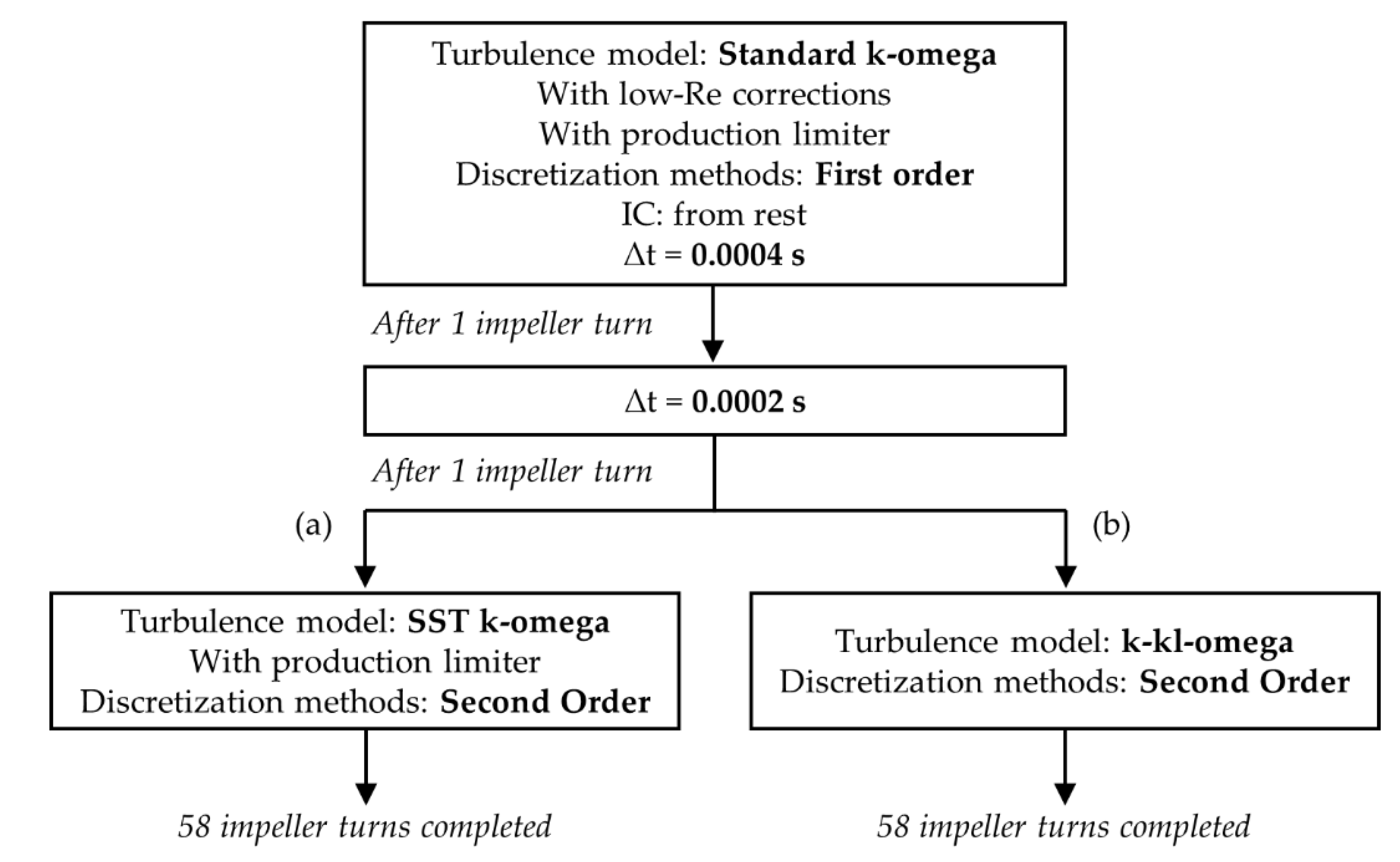
3.3. CFD Settings Analysis
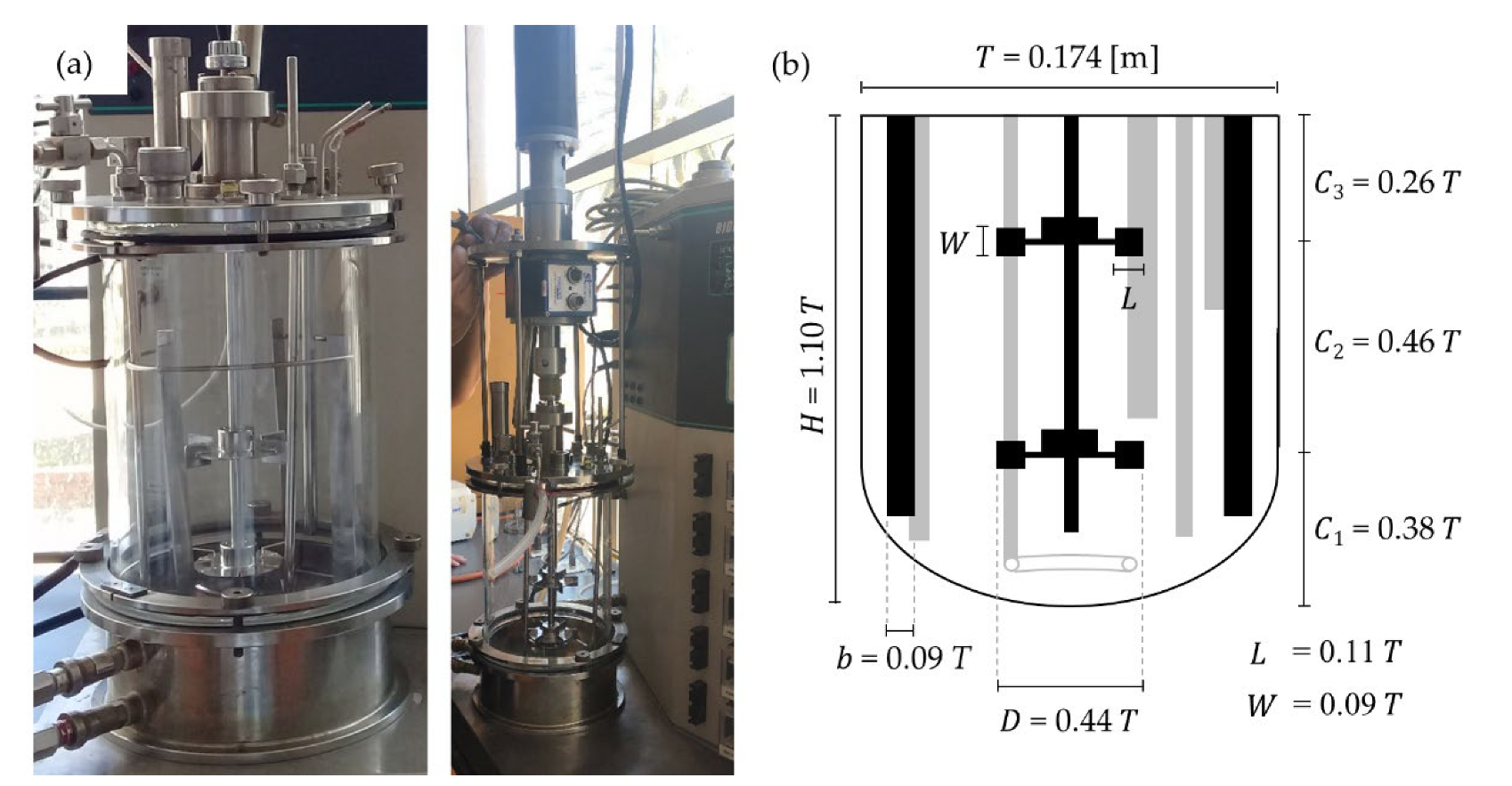
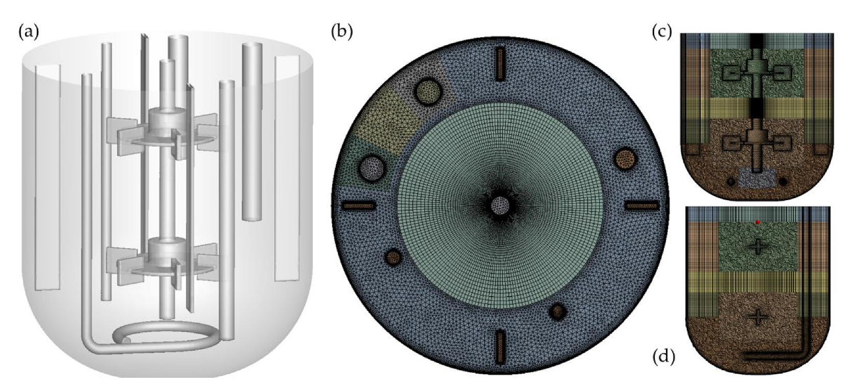
For an accurate simulation of the mixing process, we have included all of the internal elements of the bioreactor in the CFD domain, even the probes that are usually neglected because we have previously proved that they affect the fluid flow patterns [
23]. Furthermore, to have an insight into the macro-instabilities, transient simulations are necessary [
23,
32,
33]. All of these factors add to the complexity of the CFD model, requiring a small time-step to achieve a convergent, numerically stable, and time-step size-independent simulation. That is the reason why, with the existing computational capabilities, it is not possible to simulate the evolution of the bioprocess within a reasonable period of time and, therefore, the strategy of simulating the abiotic systems to approach the fermentation process stages remains the only realistic option for now. Indeed, to simulate 0.15 s (one impeller turn) of XSolB-SSTkω, 7.5 h of computation was required using a cluster of 64 CPUs with processors Intel(R) Xeon(R) E5-2683 v4. Thus, using the same computational resources, around1232 years would be required to simulate 60 hr of fermentation. If we consider the continuous computational improvement during that time, however, this estimation would be substantially reduced.
The residual values were verified. In the case of XSolA-SSTkω, initially, the residual for the turbulence parameter ω converged intermittently, to finally stop converging during the simulation of the sixth impeller turn, while all the other residuals were below 10−5 at every time step. For XSolB-SSTkω, all the residuals were below 10−5 at every time step, except the residual of the parameter ω in a few time steps (approximately 17 out of 750 time-steps). In the cases of XSolA-SSTkω and XSolB-SSTkω, the parameter ω stabilized around 10−5 and did not go below. For XSolA-kklω, XSolB-kklω, and XSolC-lam, the residuals values were below 10−5 at every time step. Furthermore, based on the monitored variables, numerical instabilities were discarded, and it was ensured that the systems were in a stationary state over the last ten impeller turns.
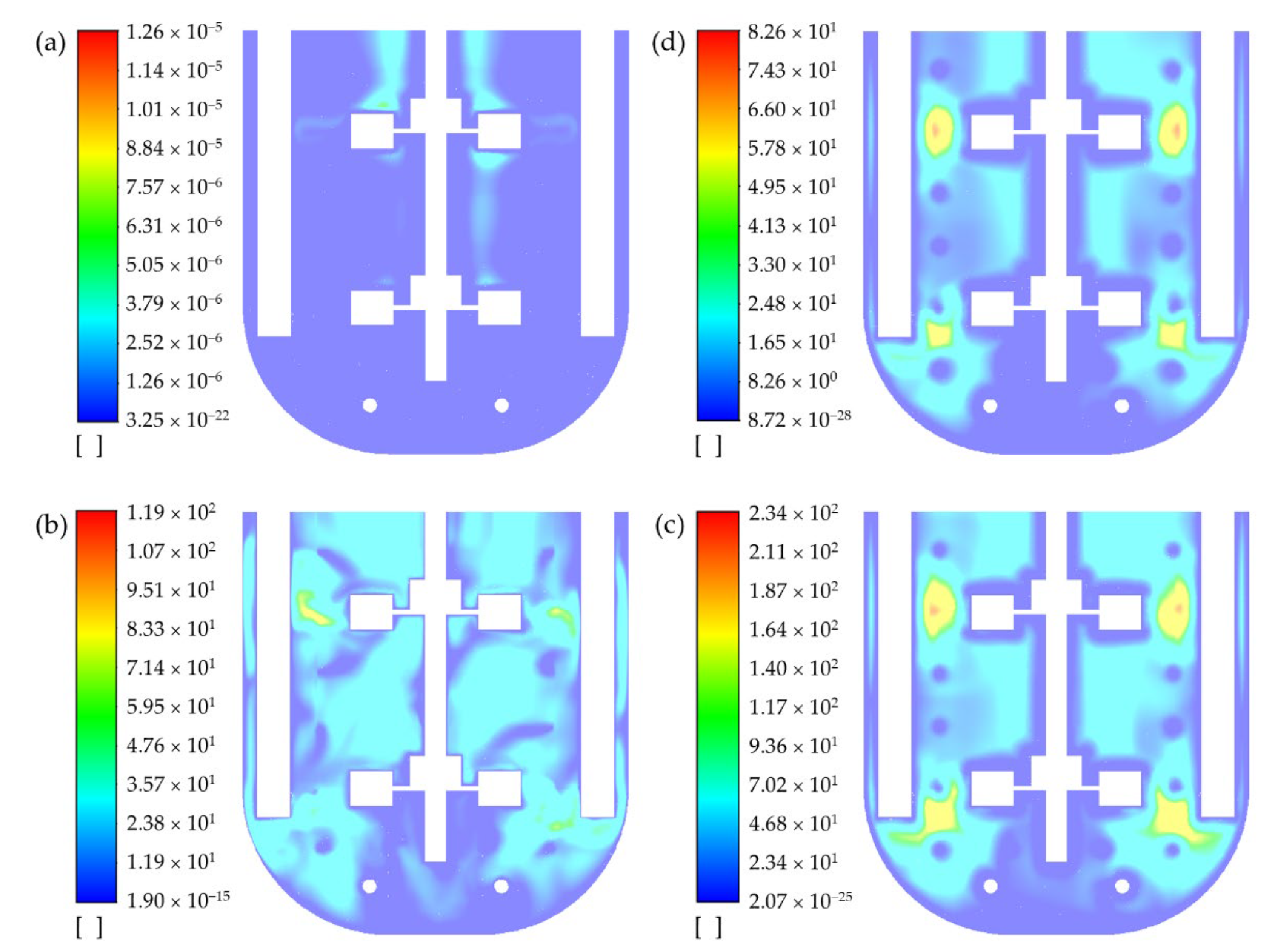
According to the analysis of the Reynolds number, the systems with Xanthan Sol C, Xanthan Sol B, and Xanthan Sol A are all in the transitional flow regime (10 ≤
≤ 10
4). However, the analysis of the turbulent viscosity ratio permitted a different conclusion (see
Appendix F). For this study, it was accepted, as a rule of thumb, that a turbulent viscosity ratio above 10 and below 5 indicates, respectively, a turbulent and a laminar flow regime, while a value between 5 and 10 corresponds to a transitional regime. Therefore, for Xanthan Sol C, even though
= 312, the flow actually corresponds to a laminar regime based on the turbulent viscosity ratio. In the case of Xanthan Sol A, the turbulent viscosity ratio values have a broader distribution, spanning the three flow regimes, but the zones in the laminar and transitional regimes prevail. As previously described, the simulation XSolA-SSTkω had convergence issues related to the parameter ω, which has been attributed to the use of a turbulent model to characterize a system where the turbulent regime is not predominant. In consequence, the model XSolA-SSTkω was discarded, and only XSolA-kklω was used to study the system Xanthan Sol A. The k-kl-omega model was chosen because it is suitable for systems where the boundary layer transitions between the laminar and turbulent regimes [
34], as happens in most of the walls of the tank due to the periodical passage of the blades and the high pseudoplasticity of Xanthan Sol A.
With respect to Xanthan Sol B, the turbulent viscosity ratio values span the three flow regimes as well, but the turbulent regime is more prevalent than for Xanthan Sol A. So much so that the results obtained with XSolB-SSTkω and XSolB-kklω are very similar, in agreement with the fact that the Reynolds number of Xanthan Sol B is very close to the limit between the transitional and turbulent range. As there is not enough information to ensure which one of the models adapted for Xanthan Sol B is better than the other one, the results of both are considered in this study. It is hypothesized that, probably, the real behaviour of the system Xanthan Sol B is at some point in between the predictions of XSolB-SSTkω and XSolB-kklω.
It is important to remark that the RANS turbulence models available in Ansys Fluent were not developed to describe the flow of non-Newtonian fluids. Their inaccuracy relies on the use of the resolved-scale strain rate instead of the local one to compute the apparent viscosity of the fluid. Unfortunately, there are few developments that could be applied for the modelling of turbulent non-Newtonian fluid flows. Gavrilov and Rudyak [
35] have proposed a new turbulence model to be used with power-law non-Newtonian fluids, but it has not been validated for stirred tanks. Instead, in recent publications of CFD models in bioprocesses as well as other fields, the traditional RANS equations have been applied to simulate the flow of non-Newtonian fluids with successful experimental validation [
9,
17,
36]. Particularly, for the case of stirred tanks, it has been shown that the SST k-omega model allows an accurate prediction of torque and flow patterns when mixing non-Newtonian fluids in the turbulent flow regime [
18,
19,
20]. However, to our knowledge, the use of k-kl-omega has not been reported for non-Newtonian fluids.
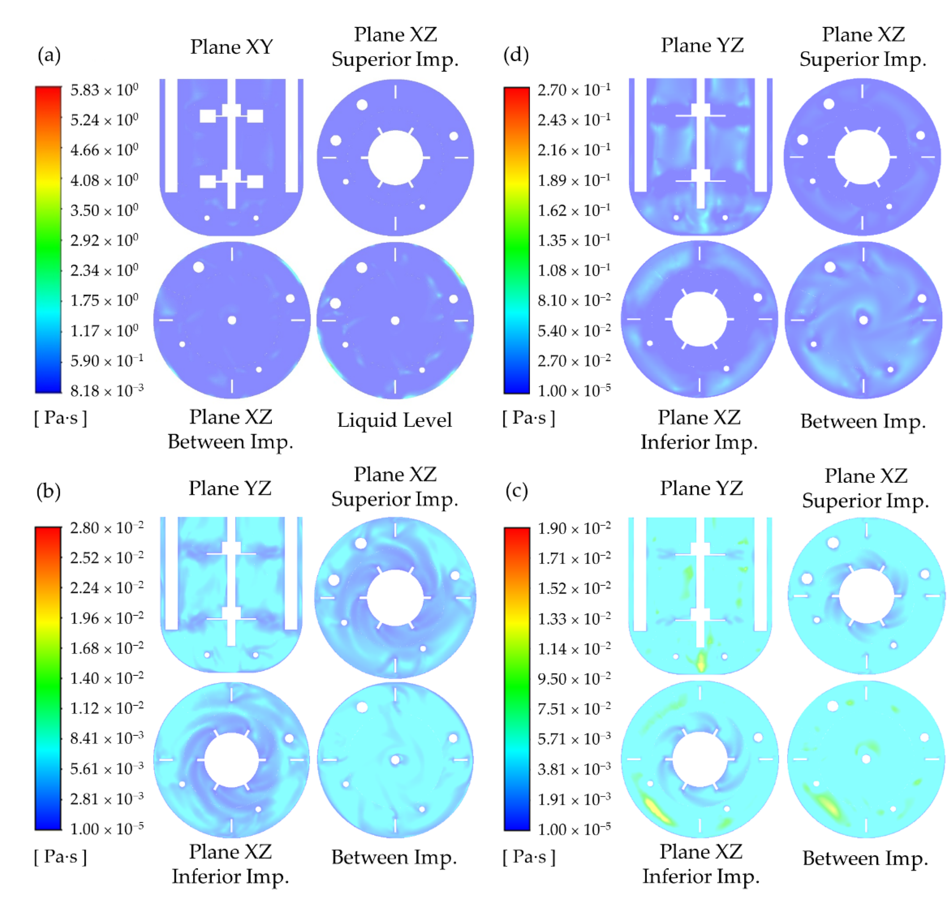
As mentioned before, ANSYS Fluent requires as input a lower and upper viscosity limit for the non-Newtonian power-law model. In other words, a power-law fluid is handled similarly to a Carreau fluid [
37]. Therefore, it is important to set up limits that will not artificially influence the simulation of the mixing system. This was evident in the case with Xanthan Sol C, for which preliminarily the upper limit was set as 0.5 Pa·s. However, after the simulation of several impeller turns, the contours at different planes showed that the viscosity reached the maximum allowed value in several zones (see
Appendix G). This observation raised the question of whether the applied upper limit was too low. During the experimental characterization of Xanthan Sol A, the maximum measured viscosity was 0.2 Pa∙s at a shear rate of 0.36 s
−1, but lower shear rates can be found in the bioreactor and, therefore, higher viscosities. According to the literature, Xanthan solutions can reach viscosities up to 8 and 200 Pa∙s at 0.1 and 0.001 s
−1, respectively [
38,
39]. Based on this, the simulation for Xanthan Sol C was re-started, using 300 Pa∙s as the upper limit. Similar attention was given to the lower viscosity limit. Thus, it was ensured that the applied viscosity limits did not affect the results obtained with the models of the abiotic systems with non-Newtonian fluids. See viscosity contours in
Appendix G.
3.4. Mesh Analysis and CFD Model Validation
The mesh independence was thoroughly proven for Water-SSTKω in previous work [
23]. So, as the models for the systems with non-Newtonian fluids used the same mesh, only the confirmation of their mesh independence was pending. As expected for grid-independent results, we found small differences between the computed values of the torque on the moving walls versus on the stationary walls responding to the conservation of angular momentum. The highest difference was 4.3%, which is similar to the one obtained for Cortada-Garcia et al. [
40] for its optimal grid. The detailed results of this analysis can be found in
Appendix H.
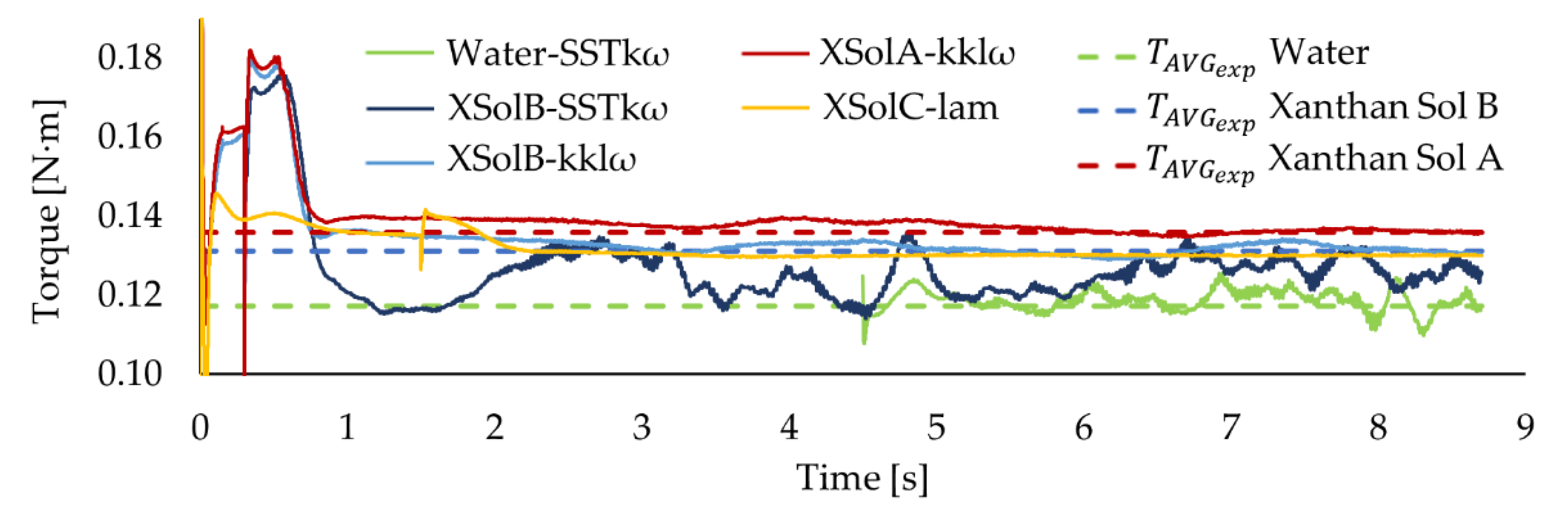
Observing
Figure 7, it is apparent that the CFD models successfully predicted the effect that the fluid viscosity has on the torque. In particular, the models XSolA-kklω and XSolB-kklω satisfactorily captured the effect of the fluid rheology on the torque for the non-Newtonian systems in the transitional flow regime. This is a relevant result because, to the best of our knowledge, it is the first time that the k-kl-omega transition model has been evaluated for the simulation of stirred tanks.
The validation analysis of Water-SSTKω can be found in Sadino-Riquelme et al. [
23]. In the case of the abiotic system with non-Newtonian fluids,
was compared with
, obtaining
below 5% (see
Table 5). These are small errors in comparison to the ones obtained by Ebrahimi et al. [
41], which vary between 5.7% and 14.9% for the simulations of dual impellers mixing water with
between 11,700 and 35,000. It is important to notice that the cited study used power values for validation purposes, which is analogous to using torque, based on their linear relationship.
Previously, for the verification analysis of the model Water-SSTkω,
was estimated as equal to 8.2% [
23]. Assuming that the validation uncertainty is the same for the abiotic systems with non-Newtonian fluids, and as
in all the cases, the CFD models for Xanthan Sol A and Xanthan Sol B are successfully validated at an 8.2% uncertainty level.
In the case of XSolC-lam, although not having experimental data to compare with, a higher comparative error related to the use of a multi-phase model with single-phase conditions can be expected. In a preliminary study, the mechanical mixing of water was simulated using the same domain described in this article to compare a single-phase CFD model versus a CFD multi-phase model under single-phase conditions. It was observed that the comparative error estimated for the multi-phase model was between 2-fold and 2.5-fold bigger than for the single-phase model. Additionally, it is interesting to notice that a lower torque was predicted for Xanthan Sol C than for Xanthan Sol A and Xanthan Sol B. Considering that Xanthan Sol C has a significantly higher viscosity than the other fluids, this result may appear erroneous, but it is not. Actually, it is in agreement with the power number curve behaviour, as Xanthan Sol C has
= 236, which corresponds to a power number smaller than for the other systems and, therefore, to a smaller torque (see
Figure 6). Thus, the model XSolC-lam is assumed as valid too.
Thus, different single-phase CFD model configurations were successfully adapted to model a stirred tank without aeration, which are able to simulate changing fluid rheology as well as an evolving flow regime.
3.5. Analysis of Mixing Mechanisms
Based on the analysis of the flow regime, it can be expected that the mixing process of the system with Xanthan Sol C will depend more on the micromixing than on the macro or mesomixing scales, contrary to what is predicted for the other systems. A comparative analysis of the turbulence length scale and Kolmogorov scale also supports that hypothesis (see
Table 5). Furthermore, the Kolmogorov scale for Xanthan Sol B (as mentioned before, it is hypothesized that the real behaviour of the system Xanthan Sol B is at some point in between the predictions of XsolB-SSTkω and XsolB-kklω), as well as for water, would be around 50% lower than for Xanthan Sol A. This would explain a significantly higher mixing time of the system Xanthan Sol A in comparison to the other systems experimentally studied. It is important to remark that the length scales are not reported for XSolC-lam because this analysis does not apply for laminar flows.
The Schmidt number allows us to compare the viscous diffusion with the molecular diffusion (see
Table 5). For alginate aqueous solutions, with alginate concentration between 0.25 and 2% (
w/
w), the oxygen diffusion coefficient varies only 14%, according to the experimental data reported by Ho et al. [
28], with an average value of 1.96∙10
−9 m
2/s. Therefore, we could expect a similar value for this parameter over the fermentation process. However, the kinematic viscosity increases 1800% from water to Xanthan Sol A (see
Table 5). Thus, even if the oxygen diffusion coefficient increases over the process due to the effect of certain broth compounds, we could still expect that the mixing will be significantly limited by the viscous diffusion.
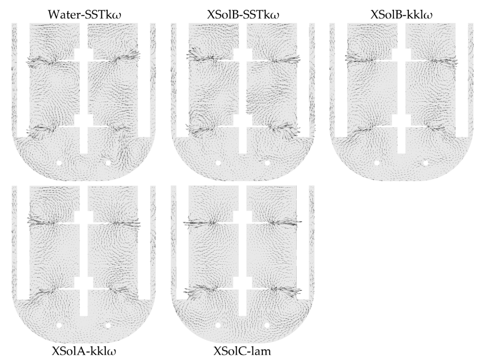
The velocity vectors of the systems were compared with those described by Rutherford et al. [
42] for stable flow patterns in a dual-Rushton turbine stirred vessel. Based on the behaviour of the vectors between the impellers and at the bottom of the fermenter, it is concluded that the systems with water and Xanthan Sol B do not have stable flow patterns, while the system with Xanthan Sol C has a parallel stable flow. In the case of Xanthan Sol A, the criterion of a parallel pattern is met by the zone between the impellers but not by the bottom zone (see
Figure 8). The flow patterns can also be studied from the examination of the lower and upper impeller torque. Both torque values are expected to be similar in a system with a parallel flow, meaning that the impellers are working independently of each other. As expected, this condition is only fulfilled by Xanthan Sol C (see
Appendix I).
The flow patterns are of importance because they affect the mixing time. Among the stable patterns, a parallel flow would have the weakest interchange between the upper and lower zones of the tank, increasing the mixing time [
42].
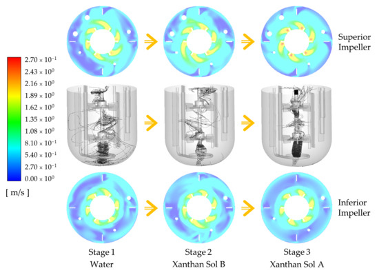
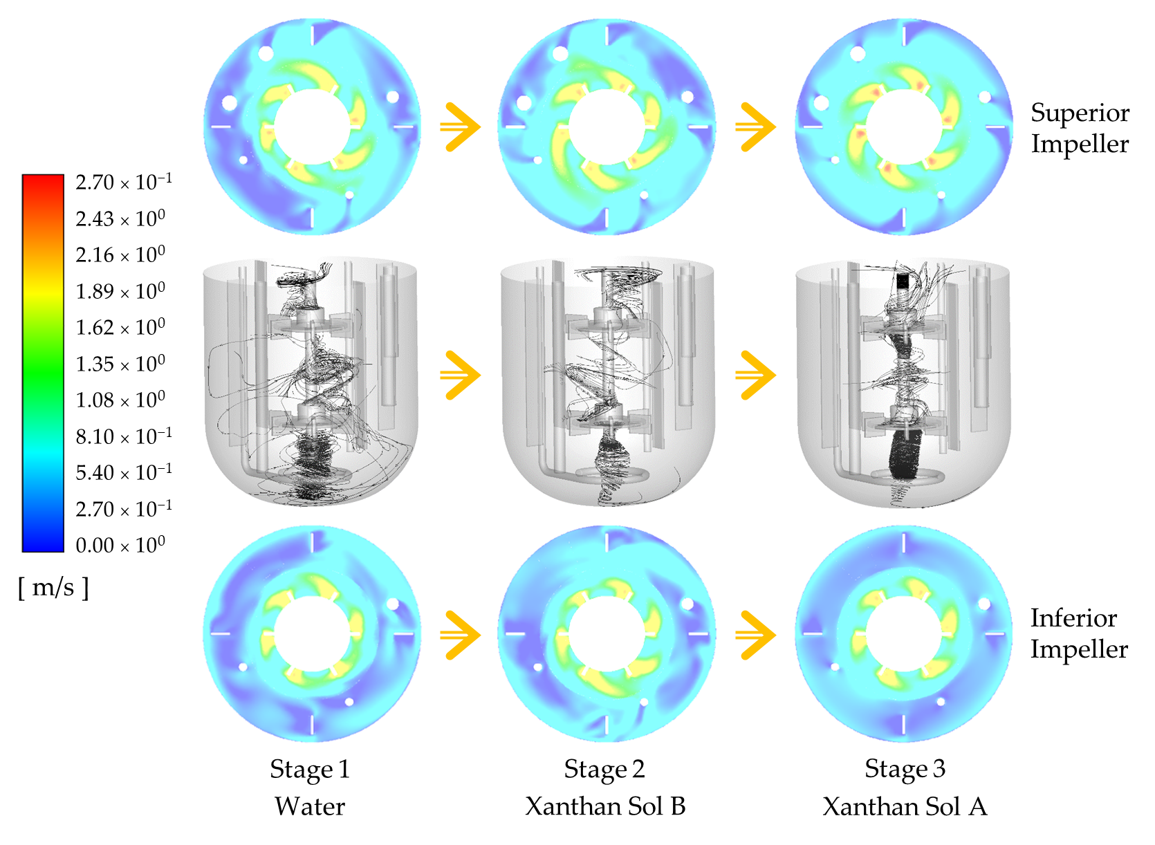
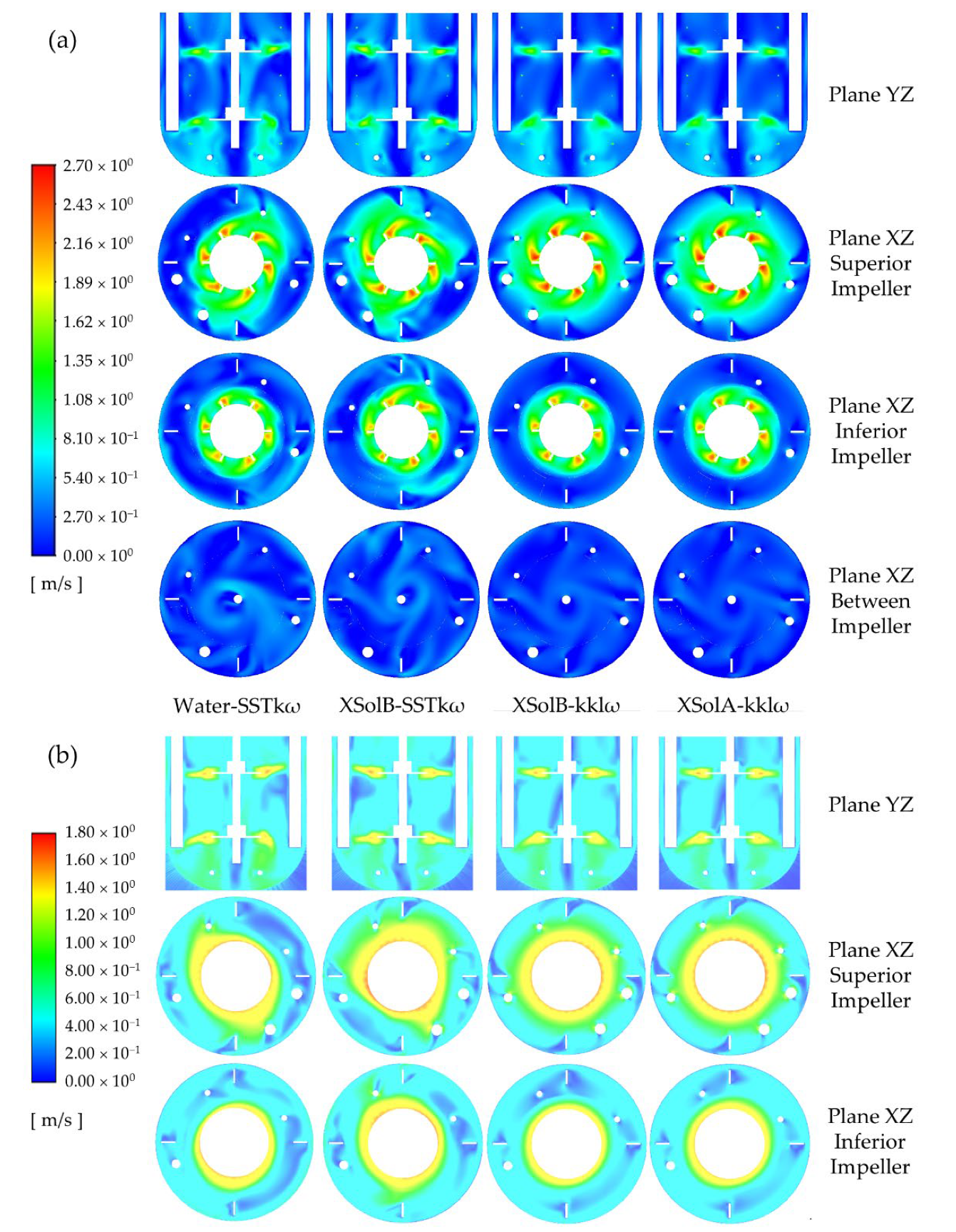
Among the three abiotic systems experimentally studied, the velocity not only changed in direction but also in magnitude. A comparative analysis of the instantaneous velocity magnitude contours shows a significant reduction of the velocity close to the walls, the liquid surface, and between the impellers, as the fluid becomes more pseudoplastic (see
Figure 9a); while the time-averaged contours reveal that the higher velocities span less area, but more symmetrically, around the impellers (see
Figure 9b). The latter is a consequence of the direction of the impeller discharge stream. The impeller discharge stream for the system with water has axial and radial components, while it is mostly radial for the other fluids.
In terms of the mixing time, that may not be detrimental for the system Xanthan Sol B, but it is a disadvantage for the case with Xanthan Sol A. Adding an axial component to the impeller discharge stream of Xanthan Sol A could help to reduce the stagnant zones and mixing time.
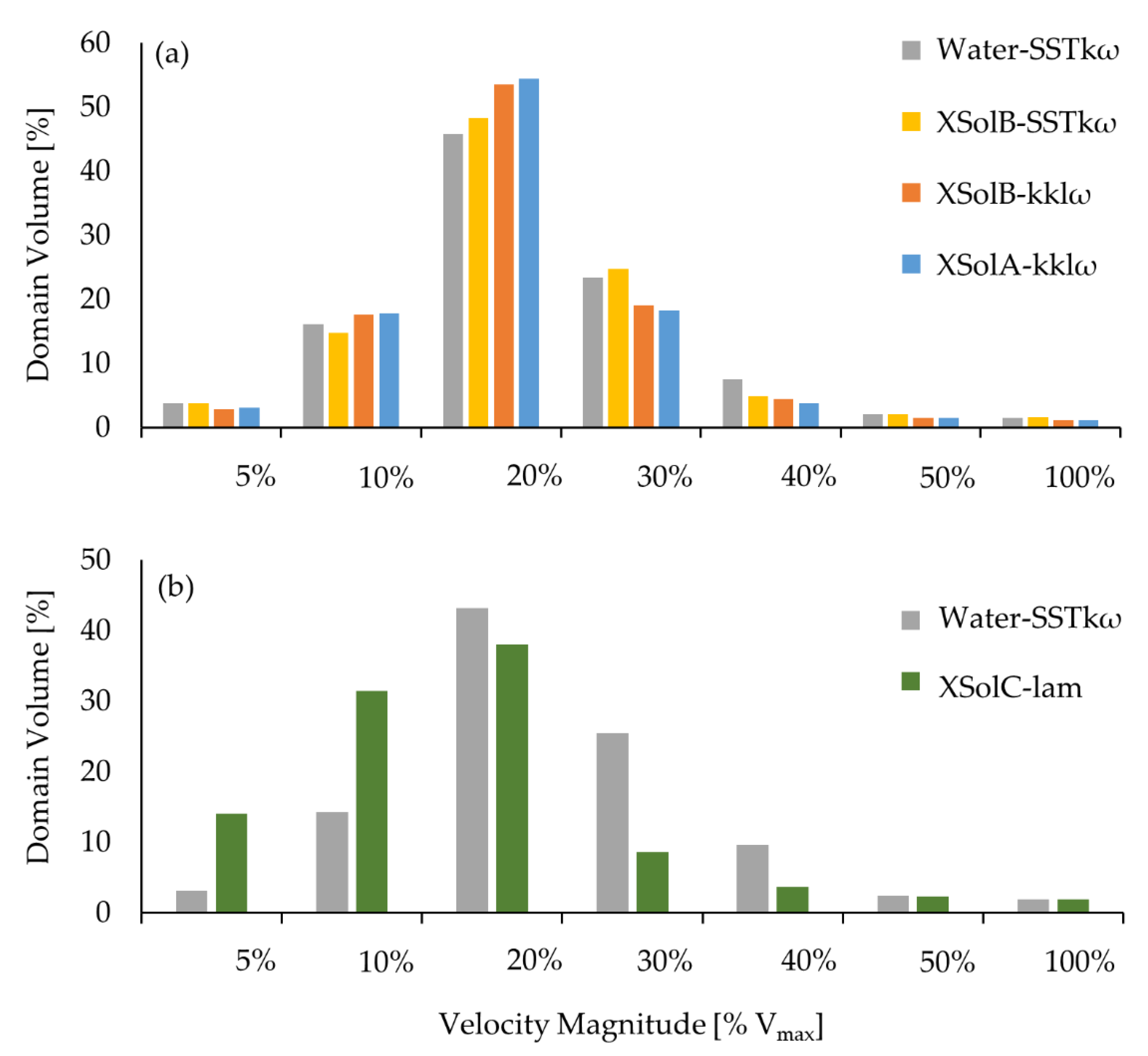
Over the course of the fermentation, an additional factor can impair the homogenization of the system, which is the stagnation of the fluid into dead zones. In this work, the definition of the dead zone used by Vesvikar and Al-Dahhan [
43] was applied. This definition considers the zones with velocity magnitude lower than 5% of the maximum velocity magnitude of the system (
). Based on this concept, when the broth properties evolve from water to Xanthan Sol B and Xanthan Sol A, although there is a significant increment of fluid volume with velocities below 20%
, it does not significantly affect the dead zone volume. On the other hand, if the broth properties evolve to Xanthan Sol C, the dead zones span 14% of the system volume, which is almost 5-fold bigger than for water. See graphics in
Appendix J.
The rotation of the Rushton turbines creates several vortical structures that enhance the mixing process by creating flow instabilities. The trailing vortices are formed just behind the blades and affect the flow due to their periodic passage (see
Figure 10a,b). For the systems with Xanthan solutions, the trailing vortices dissipated at a shorter radial distance from the shaft than for the case with water due to the higher viscosities that dissipate the eddies into heat. Moreover, the vertical distance between the trailing vortices of each blade is stretched as higher the pseudoplasticity. Overall, the superior impeller vortices are slightly different from those of the inferior one as an effect of the tank’s internal elements.
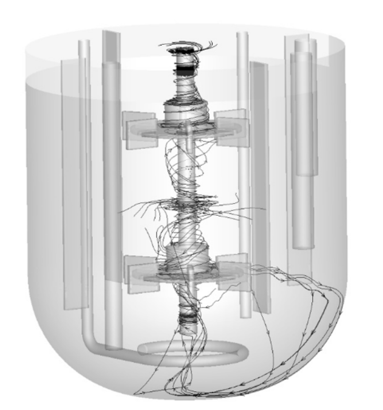
An additional vortical structure was found around the impeller axis (see
Figure 10c). It is an effect of a phenomenon called the Ekman Layer, where the pressure gradient force, the Coriolis force and the turbulent drag play a fundamental role. The difference between the vorticity in the bulk of the fluid and the tank bottom generates a vertical velocity that, in these systems, pumps the fluid upwards (see
Figure 10d). This is called Ekman pumping, and it can be associated with a precessional vortex type of macro-instability [
44]. This feature is an advantage when there are particles that need to be suspended, such as the microorganisms inside the bioreactor. Furthermore, the unstable flow patterns of the abiotic systems with water and Xanthan Sol B can be explained by the behaviour of these vortices, especially by its asymmetric shape around the shaft, in the zone between the impellers. Congruently, the parallel flow pattern was related to a symmetric vortex around the impeller axis (see
Appendix K). Furthermore, the vortex around the impeller axis would explain the flow pattern differences observed in the tank bottom when comparing the vortex shape Xanthan Sol C with the other abiotic systems.
Other vortical structures are formed around the probes, baffles, and sparger (see
Figure 10e). It is important to highlight the existence of these vortices because, most of the time, these elements are not included in the CFD domain. However, as shown here, they play a role in the fluid dynamics at a mesomixing scale.
Based on the experimental and computational results, it is hypothesized that the aeration would modify the trailing vortices and the Ekman pumping by the onset of the air cavities and the modification of the pressure gradients in the bottom zone of the tank, respectively. Currently, the CFD models with aeration are being adapted to study the veracity of these hypotheses.
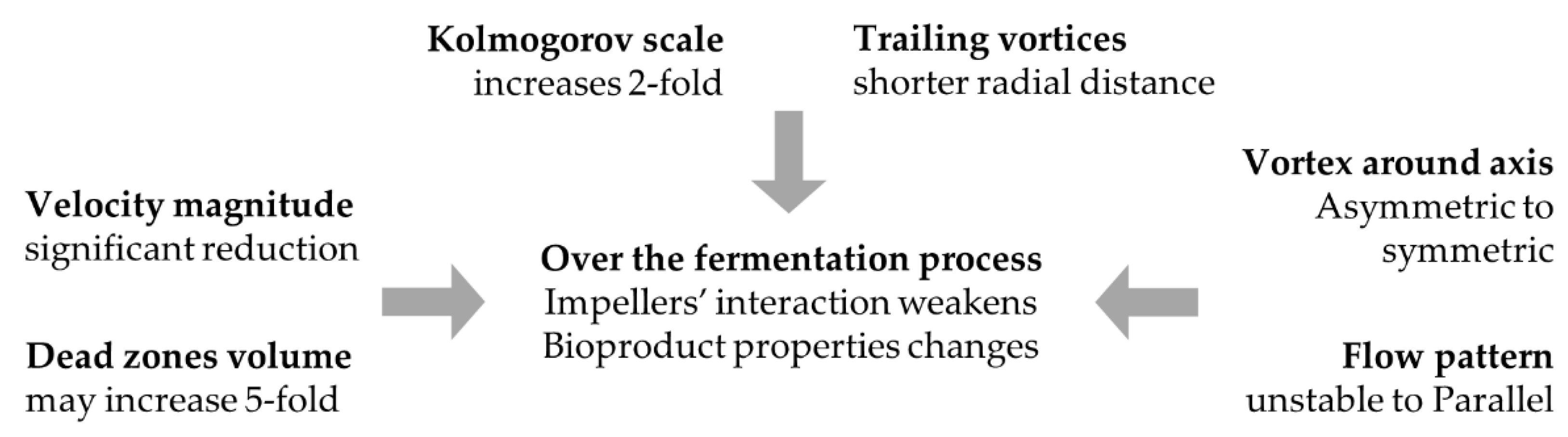
Figure 11 summarizes the modifications that the fluid dynamics of a bioprocess with evolving pseudoplasticity can be subjected to that may impair the fermentation results. Importantly, all these factors were characterized using CFD modelling, which implies that CFD-aided design can be applied to optimize the mixing mechanisms of stirred bioprocesses with changing fluid rheology. For example, the effect of the position of probes, impellers, and air injection on the vortical structures could be studied to identify a tank configuration that improves the mixing times and biomass suspension. Furthermore, the CFD configurations described in this work would allow the study of the optimization of the fluid dynamics based on the specific needs of the different fermentation stages. For example, variable operating conditions could be analyzed in order to counteract the rheology changes.


 ,
, 


