Shifts in Forest Structure in Northwest Montana from 1972 to 2015 Using the Landsat Archive from Multispectral Scanner to Operational Land Imager

 ,
,
Abstract
:1. Introduction
2. Materials and Methods
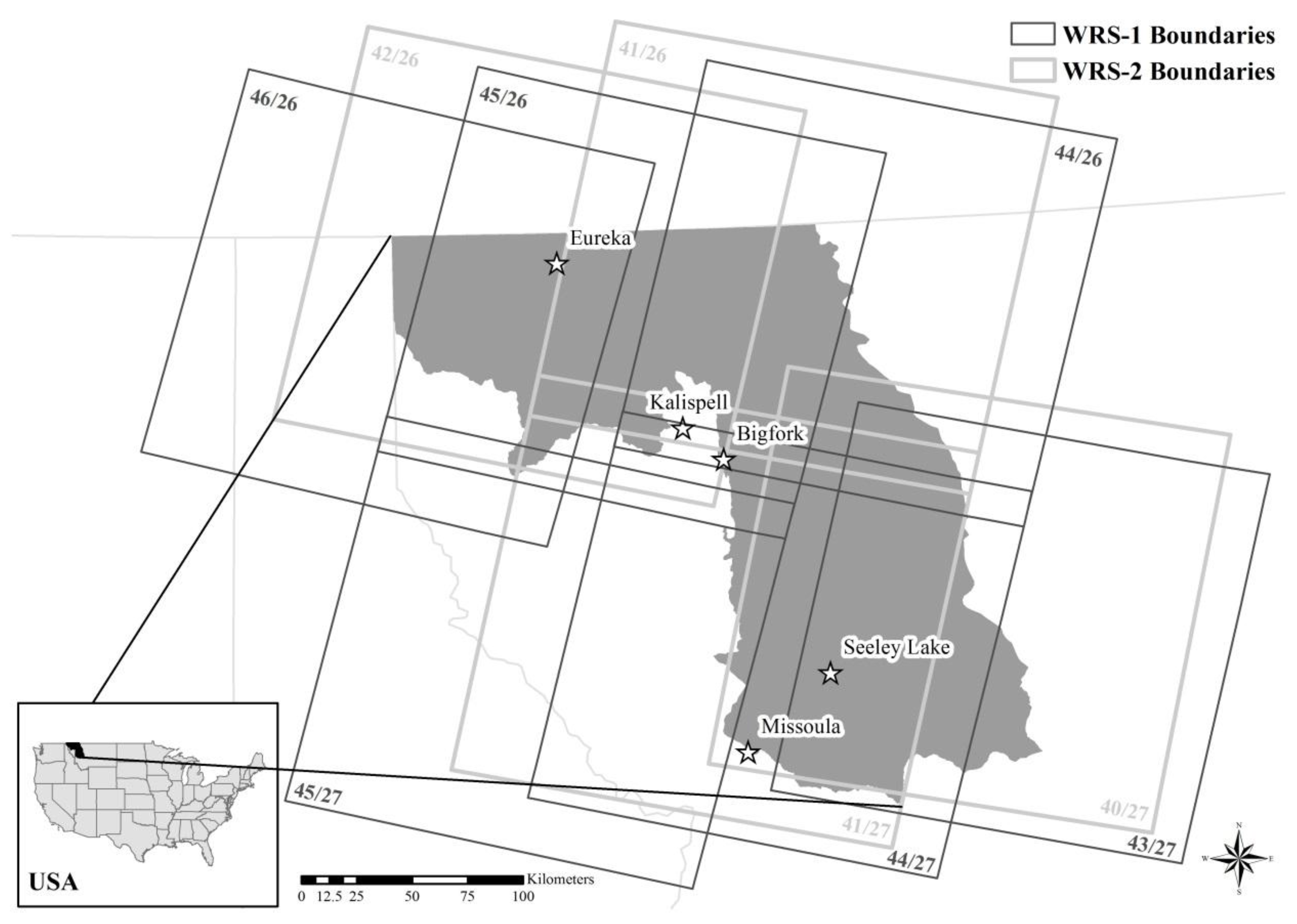
2.1. Study Area
2.2. Data Collection
2.2.1. Landsat Imagery
2.2.2. Forest Structure Reference Data
2.2.3. Ancillary Data
2.3. Landsat Data Processing through LandsatLinkr
2.4. Ancillary Data Processing
2.5. Classification of Master Image
2.5.1 Accuracy Assessment of the Initial 2013 Classification
2.6. Change Vector Analysis
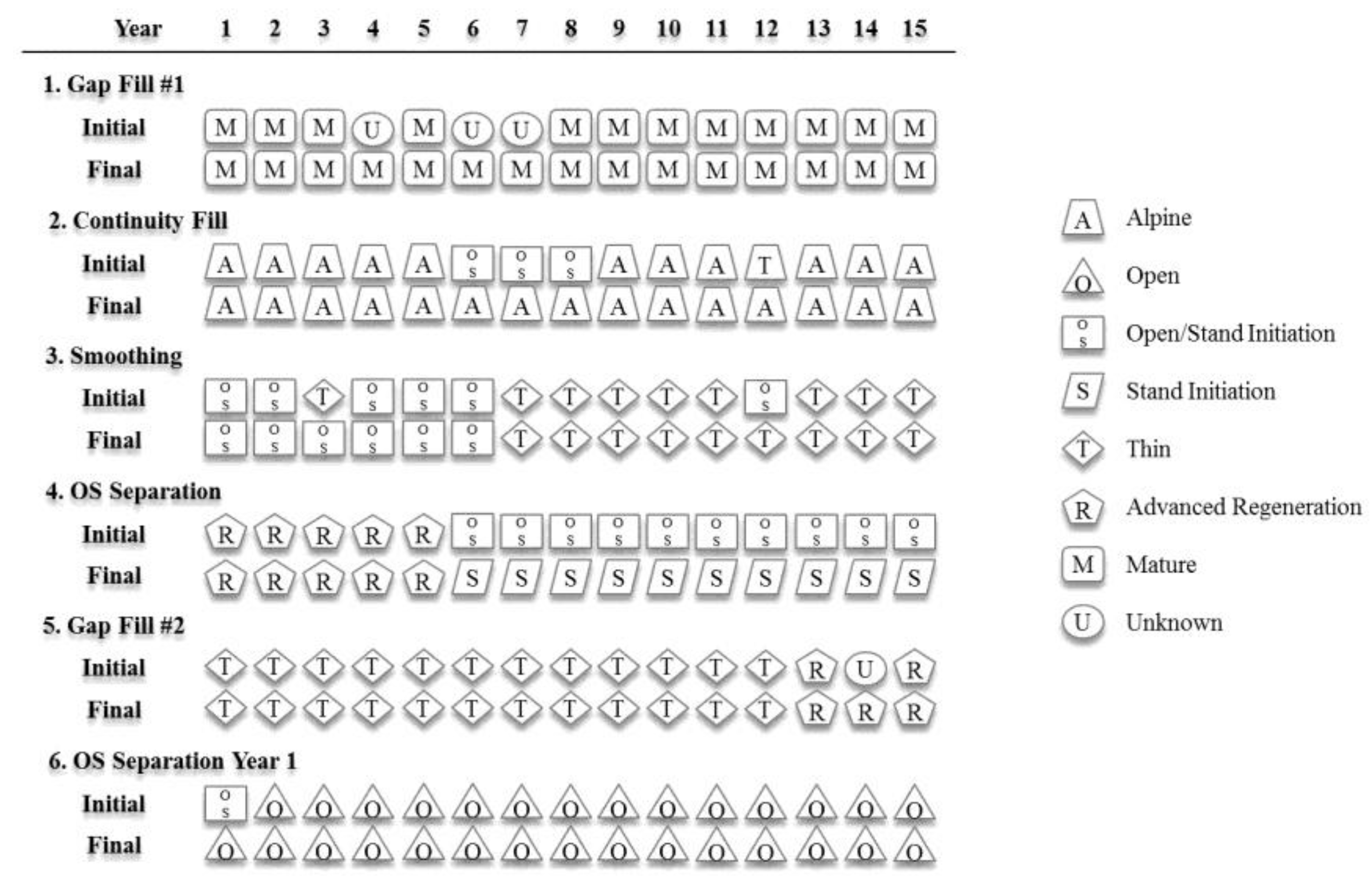
2.7. Informing Yearly Classifications with Time Series
- Gap fill #1 (where no data existed in a year—due to clouds, scan line gaps, and/or missing scenes for that year): utilized data from surrounding years by filling with the class of the previous year if it was not Unknown, or with the following year if the class of the previous year was Unknown; remained Unknown if the classes of the surrounding years were Unknown;
- Continuity fill: looked for consistent Alpine, Mature, and Open/Stand Initiation (i.e., 1972 = A, 2015 = A, and the majority of the time series at this pixel = A, then fill this pixel with A);
- Smoothing: looked for single occurrences within the time series (i.e., if 1973 = Thin, 1974 = Open/Stand Initiation, and 1975 = Thin, fill the 1974 pixel with Thin);
- Separate Open from Stand Initiation: based on whether previous years were Mature, Advanced Regeneration, or Thin (we expect that Open would not follow Mature, Advanced Regeneration, or Thin directly, while Stand Initiation can follow them directly); does not include any changes to 1972;
- Gap fill #2: utilized data from surrounding years by filling with the class of the previous year if it was not Unknown, or with the following year if the class of the previous year was Unknown; remained Unknown if the classes of the surrounding years were Unknown;
- Separate Open from Stand Initiation for the 1972 classification: based on 1973 values;
- Alpine by elevation (any Open pixel ≥ 2500 m was labeled as Alpine);
- Mask low elevation to exclude areas of non-forest (exclude all pixels <500 m).
2.8. Accuracy Assessment for Initial and Time-Series-Informed Classifications
2.9. Comparison to US Forest Service Forest Inventory and Analysis Data
3. Results
3.1. Classification of Master Image
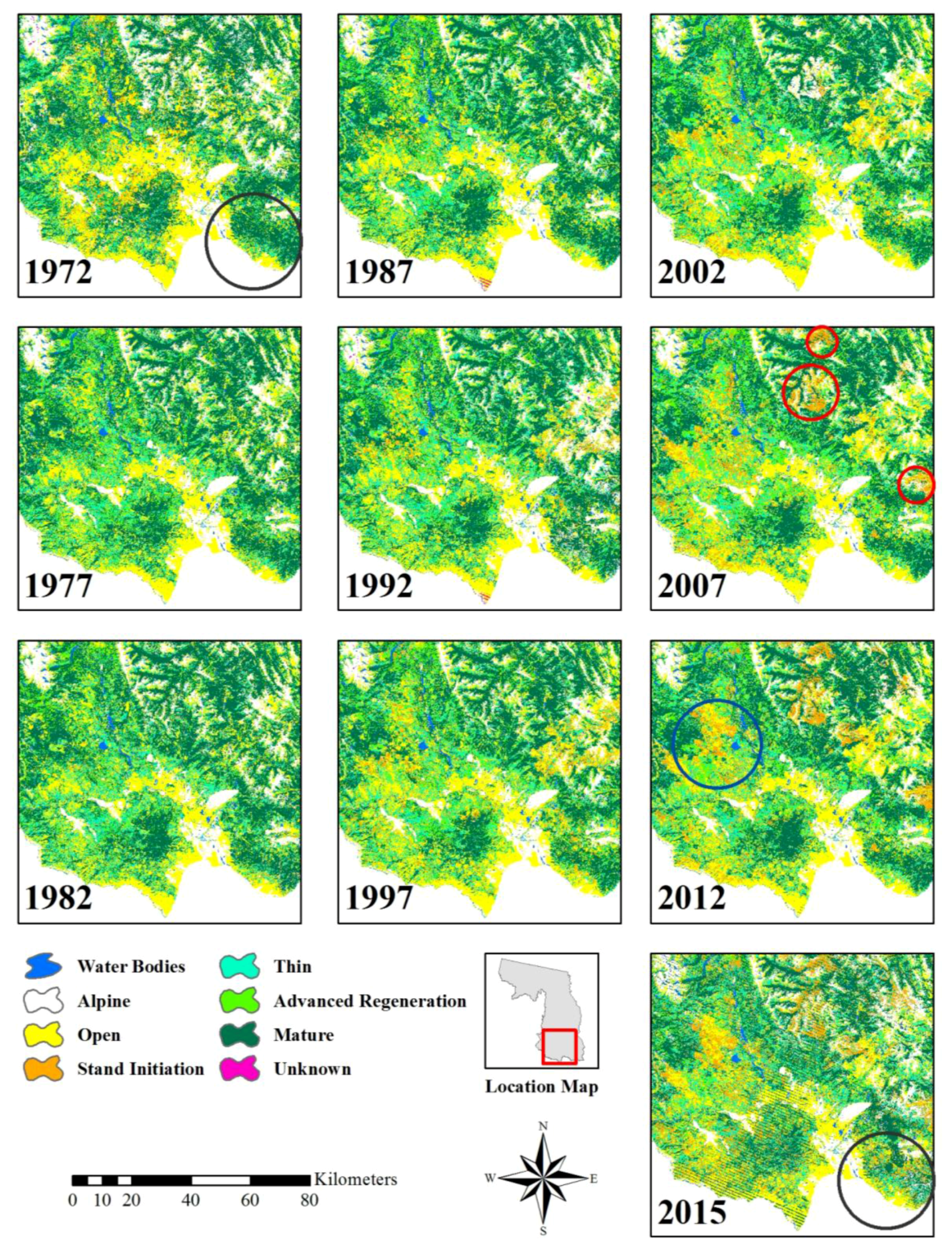
3.2. Yearly Forest Structure Classifications
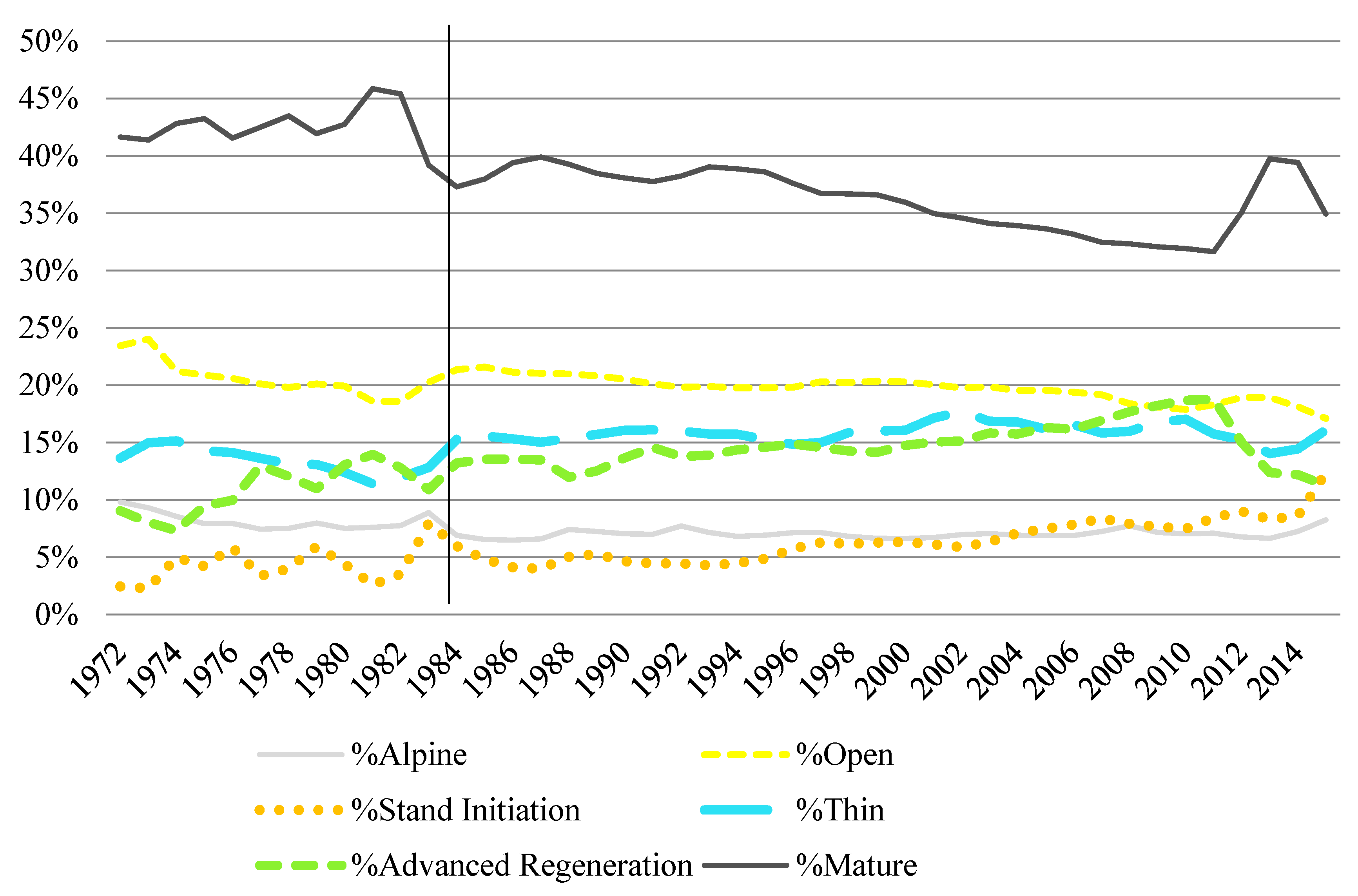
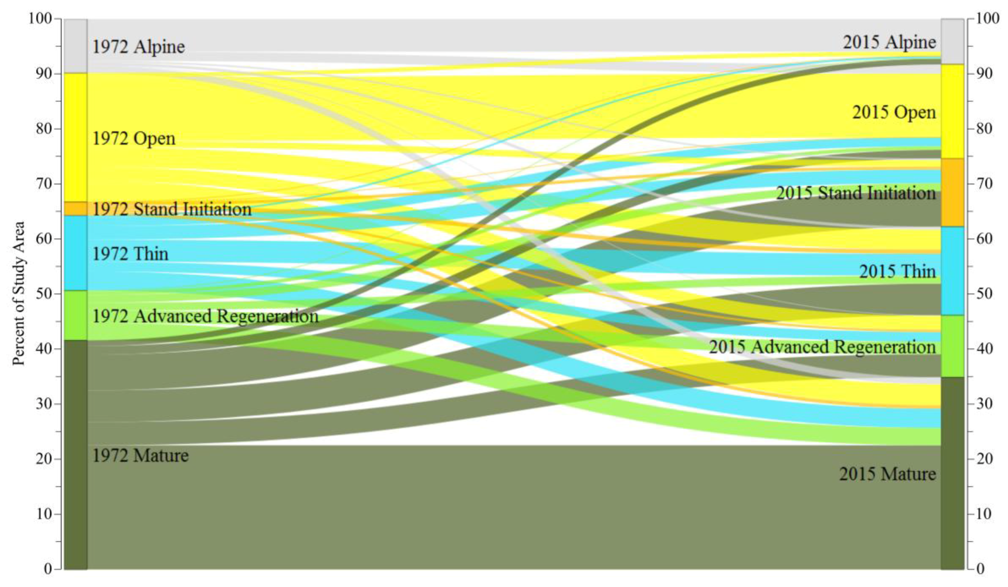
3.3. Time-Series-Informed Yearly Classifications
4. Discussion
4.1. Time Series Analysis
4.2. Classification of Forest Structure
4.3. Change Vector Analysis and Temporal Continuity Rules
5. Conclusions
Supplementary Materials
Acknowledgments
Author Contributions
Conflicts of Interest
References
- Cazcarra-Bes, V.; Tello-Alonso, M.; Fischer, R.; Heym, M.; Papathanassiou, K. Monitoring of forest structure dynamics by means of L-band SAR tomography. Remote Sens. 2017, 9, 1229. [Google Scholar] [CrossRef]
- DeVries, B.; Verbesselt, J.; Kooistra, L.; Herold, M. Robust monitoring of small-scale forest disturbance in a tropical montane forest using Landsat time series. Remote Sens. Environ. 2015, 161, 107–120. [Google Scholar] [CrossRef]
- Hill, R.A.; Hinsley, S.A. Airborne lidar for woodland habitat quality monitoring: Exploring the significance of lidar data characgteristics when modelling organism-habitat relationships. Remote Sens. 2015, 7, 3446–3466. [Google Scholar] [CrossRef]
- Lefsky, M.A.; Cohen, W.B.; Spies, T.A. An evaluation of alternate remote sensing products for forest inventory, monitoring, and mapping of Douglas-fir forests in western Oregon. Can. J. For. Res. 2000, 31, 78–87. [Google Scholar] [CrossRef]
- Noss, R.F. Assessing and monitoring forest biodiversity: A suggested framework and indicators. For. Ecol. Manag. 1999, 115, 135–146. [Google Scholar] [CrossRef]
- Kennedy, R.E.; Yang, Z.; Cohen, W.B. Detecting trends in forest disturbance and recovery using yearly Landsat time series: 1. LandTrendr—Temporal segmentation algorithms. Remote Sens. Environ. 2010, 114, 2897–2910. [Google Scholar] [CrossRef]
- Cohen, W.B.; Yang, Z.; Kennedy, R. Detecting trends in forest disturbance and recovery using yearly Landsat time series: 2. TimeSync—Tools for calibration and validation. Remote Sens. Environ. 2010, 114, 2911–2924. [Google Scholar] [CrossRef]
- Brooks, E.B.; Coulston, J.W.; Wynne, R.H.; Thomas, V.A. Improving the precision of dynamic forest parameter estimates using Landsat. Remote Sens. Environ. 2010, 179, 162–169. [Google Scholar] [CrossRef]
- Braaten, J.D.; Cohen, W.B.; Yang, Z. LandsatLinkr. Zenodo 2017. [Google Scholar] [CrossRef]
- Pasquarella, V.J.; Bradley, B.A.; Woodcock, C.E. Near-Real-Time Monitoring of Insect Defoliation Using Landsat Time Series. Forests 2017, 8, 275. [Google Scholar] [CrossRef]
- Bunker, B.E.; Tullis, J.A.; Cothren, J.D.; Casana, J.; Aly, M.H. Object-based Dimensionality Reduction in Land Surface Phenology Classification. AIMS Geosci. 2016, 2, 302–328. [Google Scholar] [CrossRef]
- Pflugmacher, D.; Cohen, W.B.; Kennedy, R.E.; Yang, Z. Using Landsat-derived disturbance and recovery history and lidar to map forest biomass dynamics. Remote Sens. Environ. 2014, 151, 124–137. [Google Scholar] [CrossRef]
- Hyde, P.; Dubayah, R.; Peterson, B.; Blair, J.B.; Hofton, M.; Hunsaker, C.; Knox, R.; Walker, W. Mapping forest structure for wildlife habitat analysis using waveform lidar: Validation of montane ecosystems. Remote Sens. Environ. 2005, 96, 427–437. [Google Scholar] [CrossRef]
- Hyde, P.; Dubyah, R.; Walker, W.; Blair, J.B.; Hofton, M.; Hunsaker, C. Mapping forest structure for wildlife habitat analysis using multi-sensor (LiDAR, SAR/InSAR, ETM+, Quickbird) synergy. Remote Sens. Environ. 2006, 102, 63–73. [Google Scholar] [CrossRef]
- Lim, K.; Treitz, P.; Wulder, M.; St-Onge, B.; Flood, M. LiDAR remote sensing of forest structure. Prog. Phys. Geogr. 2003, 27, 88–106. [Google Scholar] [CrossRef]
- Zald, H.S.; Wulder, M.A.; White, J.C.; Hilker, T.; Hermosilla, T.; Hobart, G.W.; Coops, N.C. Integrating Landsat pixel composite and change metrics with lidar plots to predictively map forest structure and aboveground biomass in Saskatchewan, Canada. Remote Sens. Environ. 2016, 176, 188–201. [Google Scholar] [CrossRef]
- Zimble, D.A.; Evans, D.L.; Carlson, G.C.; Parker, R.C.; Grado, S.C.; Gerard, P.D. Characterizing vertical forest structure using small-footprint airborne LiDAR. Remote Sens. Environ. 2003, 87, 171–182. [Google Scholar] [CrossRef]
- Wulder, M.A.; Masek, J.G.; Cohen, W.B.; Loveland, T.R.; Woodcock, C.E. Opening the archive: How free data has enabled the science and monitoring promise of Landsat. Remote Sens. Environ. 2012, 122, 2–10. [Google Scholar] [CrossRef]
- Wulder, M.A.; White, J.C.; Loveland, T.R.; Woodcock, C.E.; Belward, A.S.; Cohen, W.B.; Fosnight, E.A.; Shaw, J.; Masek, J.G.; Roy, D.P. The global Landsat archive: Status, consolidation, and direction. Remote Sens. Environ. 2016, 185, 271–283. [Google Scholar] [CrossRef]
- Ahmed, O.S.; Wulder, M.A.; White, J.C.; Hermosilla, T.; Coops, N.C.; Franklin, S.E. Classification of annual non-stand replacing boreal forest change in Canada using Landsat time series: A case study in northern Ontario. Remote Sens. Lett. 2017, 8, 29–37. [Google Scholar] [CrossRef]
- Huang, C.; Goward, S.N.; Masek, J.G.; Thomas, N.; Zhu, Z.; Vogelmann, J.E. An automated approach for reconstructing recent forest disturbance history using dense Landsat time series stacks. Remote Sens. Environ. 2010, 114, 183–198. [Google Scholar] [CrossRef]
- Neigh, C.S.; Bolton, D.K.; Diabate, M.; Williams, J.J.; Carvalhais, N. An automated approach to map the history of forest disturbance from insect mortality and harvest with Landsat time-series data. Remote Sens. 2014, 6, 2782–2808. [Google Scholar] [CrossRef]
- Schroeder, T.A.; Wulder, M.A.; Healy, S.P.; Moisen, G.G. Mapping wildfire and clearcut harvest disturbances in boreal forests with Landsat time series data. Remote Sens. Environ. 2011, 115, 1421–1433. [Google Scholar] [CrossRef]
- Zhao, F.R.; Meng, R.; Huang, C.; Zhao, M.; Zhao, F.A.; Gong, P.; Yu, L.; Zhu, Z. Long-term post-disturbance forest recovery in the greater Yellowstone Ecosystem analyzed using Landsat time series stack. Remote Sens. 2016, 8, 898. [Google Scholar] [CrossRef]
- Pflugmacher, D.; Cohen, W.B.; Kennedy, R.E. Using Landsat-derived disturbance history (1972–2010) to predict current forest structure. Remote Sens. Environ. 2012, 122, 146–165. [Google Scholar] [CrossRef]
- Brown, S.; Barber, J. The Region 1 Existing Vegetation Mapping Program (VMap), Flathead National Forest Overview, version 12; Region One Vegetation Classification, Mapping, Inventory and Analysis Report 12–34; USDA Forest Service: Missoula, MT, USA, 2012. [Google Scholar]
- Kosterman, M.K.; Squires, J.R.; Holbrook, J.D.; Pletscher, D.H.; Hebblewhite, M. Forest structure provides the income for reproductive success in a southern population of Canada lynx. Ecol. Appl. 2018. [Google Scholar] [CrossRef] [PubMed]
- Crist, E.P.; Cicone, R.C. A physically-based transformation of Thematic Mapper data–The TM Tasseled Cap. IEEE Trans. Geosci. Remote 1984, 3, 256–263. [Google Scholar] [CrossRef]
- Crist, E.P. A TM tasseled cap equivalent transformation for reflectance factor data. Remote Sens. Environ. 1985, 17, 301–306. [Google Scholar] [CrossRef]
- Kennedy, R.F.; Cohen, W.B. Automated designations of tie-points for image-to-image coregistration. Int. J. Remote Sens. 2003, 24, 3467–3490. [Google Scholar] [CrossRef]
- Braaten, J.D.; Cohen, W.B.; Yang, Z. Automated cloud and cloud shadow identification in Landsat MSS imagery for temperate ecosystems. Remote Sens. Environ. 2015, 169, 128–138. [Google Scholar] [CrossRef]
- Chavez, P.S. Image-based atmospheric corrections–revisited and improved. Photogramm. Eng. Remote Sens. 1996, 62, 1025–1035. [Google Scholar] [CrossRef]
- Chavez, P.S., Jr. An improved dark-object subtraction technique for atmospheric scattering correction of multispectral data. Remote Sens. Environ. 1988, 24, 459–479. [Google Scholar] [CrossRef]
- Masek, J.G.; Vermote, E.F.; Saleous, N.E.; Wolfe, R.; Hall, F.G.; Huemmrich, K.F.; Gao, F.; Kutler, J.; Lim, T.K. A Landsat surface reflectance dataset for North America, 1990–2000. IEEE Geosci. Remote Sens. 2006, 3, 68–72. [Google Scholar] [CrossRef]
- Vermote, E.; Justice, C.; Claverie, M.; Franch, B. Preliminary analysis of the performance of the Landsat 8/OLI land surface reflectance product. Remote Sens. Environ. 2016, 185, 46–56. [Google Scholar] [CrossRef]
- Zhu, Z.; Woodcock, C.E. Object-based cloud and cloud shadow detection in Landsat imagery. Remote Sens. Environ. 2012, 118, 83–94. [Google Scholar] [CrossRef]
- Olofsson, P.; Foody, G.M.; Herold, M.; Stehman, S.V.; Woodcock, C.E.; Wulder, M.A. Good practices for estimating area and assessing accuracy of land change. Remote Sens. Environ. 2014, 148, 42–57. [Google Scholar] [CrossRef]
- Lambin, E.F.; Strahler, A.H. Change-vector analysis in multitemporal space: A tool to detect and categorize land-cover change processes using high temporal-resolution satellite data. Remote Sens. Environ. 1994, 48, 231–244. [Google Scholar] [CrossRef]
- Crookston, N.; Dixon, G. The forest vegetation simulator: A review of its structure, content, and applications. Comput. Electron. Agric. 2005, 49, 60–80. [Google Scholar] [CrossRef]
- Hais, M.; Kuĉera, T. Surface temperature change of spruce forest as a result of bark beetle attach: Remote sensing and GIS approach. Eur. J. For. Res. 2008, 127, 327–336. [Google Scholar] [CrossRef]
- Oliver, C.D. Forest development in North America following major disturbances. For. Ecol. Manag. 1980, 3, 153–168. [Google Scholar] [CrossRef]
- Shatford, J.P.A.; Hibbs, D.E.; Puettmann, K.J. Conifer regeneration after forest fire in the Klamath-Siskiyous: How much, how soon? J. For. 2007, 105, 139–146. [Google Scholar] [CrossRef]
- Swanson, M.E.; Franklin, J.F.; Beschta, R.L.; Crisafulli, C.M.; DellaSala, D.A.; Hutto, R.L.; Lindenmayer, D.B.; Swanson, F.J. The forgotten stage of forest succession: Early-successional ecosystems on forest sites. Front. Ecol. Environ. 2011, 9, 117–125. [Google Scholar] [CrossRef]
- Carlson, B.Z.; Georges, D.; Rabatel, A.; Randin, C.F.; Renaud, J.; Delestrade, A.; Zimmermann, N.E.; Choler, P.; Thuiller, W. Accounting for tree line shift, glacier retreat and primary succession in mountain plant distribution models. Divers. Distrib. 2014, 20, 1379–1391. [Google Scholar] [CrossRef]
- Gehrig-Fasel, J.; Guisan, A.; Zimmerman, N.E. Tree line shifts in the Swiss Alps: Climate change or land abandonment? J. Veg. Sci. 2007, 18, 571–582. [Google Scholar] [CrossRef]
- Grace, J.; Berninger, F.; Nagy, L. Impacts of climate change on the tree line. Ann. Bot. 2002, 90, 537–544. [Google Scholar] [CrossRef] [PubMed]
- Sauer, B.; Morfitt, R.; Dwyer, J. Landsat Product Improvement, Collection Processing and Management Update, MSS and No PCD Data, Surface Reflectance Status, U.S. Analysis Ready Data and Global Considerations. In Proceedings of the Landsat Science Team Meeting, Boston, MA, USA, 10–12 January 2017; Boston University: Boston, MA, USA, 2017. [Google Scholar]
- Savage, S.L.; Lawrence, R.L. Vegetation dynamics in Yellowstone’s Northern Range: 1985 to 1999. Photogramm. Eng. Remote Sens. 2010, 76, 547–556. [Google Scholar] [CrossRef]


| Overall Accuracy 2013 (%) | SE 2013 (%) | Overall Accuracy 2005 (%) | SE 2005 (%) | Overall Accuracy 1995 (%) | SE 1995 (%) | Overall Accuracy 1975 (%) | SE 1975 (%) | |
|---|---|---|---|---|---|---|---|---|
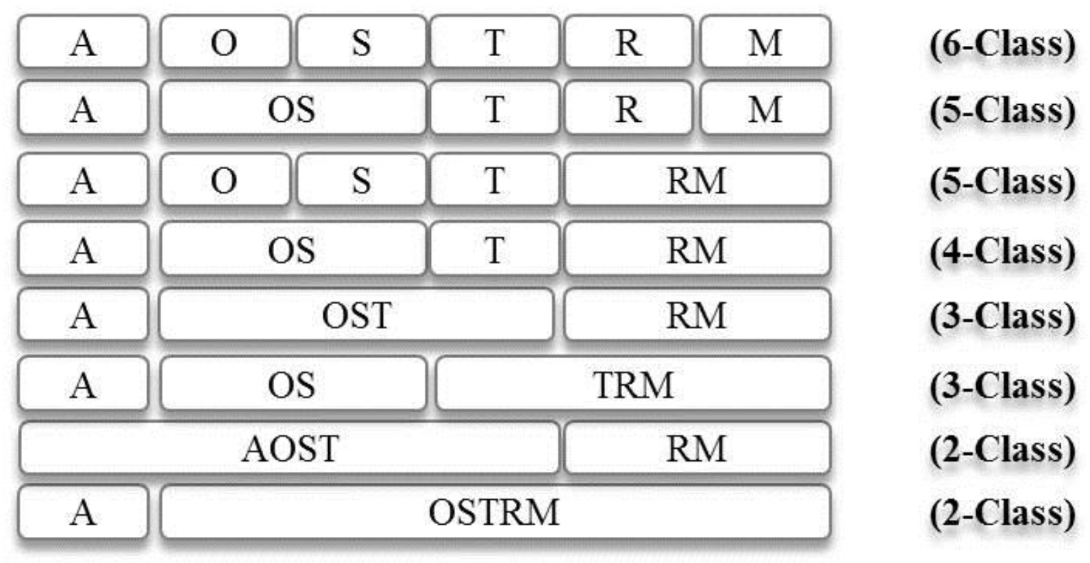
| A vs. O vs. S vs. T vs. R vs. M (6-class) | 68 | 3 | --- | --- | --- | --- | --- | --- |
| A vs. OS vs. T vs. R vs. M (5-class) | 73 | 2 | 55 | 3 | 60 | 3 | 58 | 2 |
| A vs. O vs. S vs. T vs. RM (5-class) | 78 | 2 | --- | --- | --- | --- | --- | --- |
| A vs. OS vs. T vs. RM (4-class) | 82 | 2 | 78 | 2 | 75 | 2 | 70 | 2 |
| A vs. OST vs. RM (3-class) | --- | --- | 90 | 2 | 82 | 2 | 80 | 2 |
| AOST vs. RM (2-class) | --- | --- | 93 | 2 | 87 | 2 | 83 | 2 |
| A vs. OS vs. TRM (3-class) | 91 | 1 | 84 | 2 | 87 | 2 | 83 | 2 |
| A vs. OSTRM (2-class) | 98 | <1 | 97 | 1 | 97 | <1 | 99 | <1 |
| Classification | Class Name | Producer’s Accuracy 2013 (%) | User’s Accuracy 2013 (%) | Producer’s Accuracy 2005 (%) | User’s Accuracy 2005 (%) | Producer’s Accuracy 1995 (%) | User’s Accuracy 1995 (%) | Producer’s Accuracy 1975 (%) | User’s Accuracy 1975 (%) |
|---|---|---|---|---|---|---|---|---|---|
| 6-class | A | 98 | 76 | --- | --- | --- | --- | --- | --- |
| O | 36 | 67 | --- | --- | --- | --- | --- | --- | |
| S | 82 | 50 | --- | --- | --- | --- | --- | --- | |
| T | 49 | 98 | --- | --- | --- | --- | --- | --- | |
| R | 54 | 80 | --- | --- | --- | --- | --- | --- | |
| M | 94 | 63 | --- | --- | --- | --- | --- | --- | |
| 5-class | A | 96 | 76 | 96 | 78 | 96 | 63 | 96 | 94 |
| OS | 93 | 75 | 82 | 67 | 80 | 88 | 75 | 84 | |
| T | 43 | 98 | 32 | 54 | 44 | 53 | 20 | 33 | |
| R | 54 | 80 | 30 | 42 | 28 | 35 | 8 | 12 | |
| M | 94 | 61 | 60 | 45 | 58 | 40 | 74 | 33 |
| Overall Accuracy 2013 (%) | SE 2013 (%) | Overall Accuracy 2005 (%) | SE 2005 (%) | Overall Accuracy 1995 (%) | SE 1995 (%) | Overall Accuracy 1975 (%) | SE 1975 (%) | |
|---|---|---|---|---|---|---|---|---|
| A vs. O vs. S vs. T vs. R vs. M (6-class) | 72 | 2 | 62 | 3 | 58 | 3 | 43 | 3 |
| A vs. OS vs. T vs. R vs. M (5-class) | 75 | 2 | 65 | 3 | 61 | 3 | 57 | 3 |
| A vs. O vs. S vs. T vs. RM (5-class) | 82 | 2 | 80 | 2 | 77 | 3 | 63 | 2 |
| A vs. OS vs. T vs. RM (4-class) | 85 | 2 | 83 | 2 | 80 | 2 | 76 | 3 |
| A vs. OST vs. RM (3-class) | 93 | 1 | 91 | 2 | 86 | 2 | 87 | 2 |
| AOST vs. RM (2-class) | 96 | 1 | 94 | 2 | 89 | 2 | 88 | 2 |
| A vs. OS vs. TRM (3-class) | 90 | 1 | 85 | 2 | 88 | 2 | 88 | 2 |
| A vs. OSTRM (2-class) | 97 | <1 | 97 | 1 | 98 | <1 | 100 | <1 |
| Classification | Class Name | Producer’s Accuracy 2013 (%) | User’s Accuracy 2013 (%) | Producer’s Accuracy 2005 (%) | User’s Accuracy 2005 (%) | Producer’s Accuracy 1995 (%) | User’s Accuracy 1995 (%) | Producer’s Accuracy 1975 (%) | User’s Accuracy 1975 (%) |
|---|---|---|---|---|---|---|---|---|---|
| 6-class | A | 98 | 71 | 96 | 79 | 96 | 81 | 96 | 100 |
| O | 94 | 56 | 82 | 52 | 80 | 61 | 87 | 39 | |
| S | 72 | 82 | 72 | 80 | 68 | 80 | 0 | 0 | |
| T | 43 | 100 | 34 | 66 | 46 | 65 | 20 | 50 | |
| R | 56 | 80 | 28 | 50 | 18 | 50 | 6 | 34 | |
| M | 96 | 66 | 72 | 48 | 82 | 47 | 91 | 40 | |
| 5-class | A | 98 | 71 | 96 | 79 | 96 | 82 | 96 | 100 |
| OS | 94 | 75 | 88 | 69 | 85 | 76 | 84 | 77 | |
| T | 43 | 100 | 34 | 66 | 46 | 65 | 20 | 46 | |
| R | 56 | 81 | 28 | 50 | 18 | 50 | 6 | 35 | |
| M | 96 | 66 | 72 | 48 | 82 | 47 | 91 | 40 |
© 2018 by the authors. Licensee MDPI, Basel, Switzerland. This article is an open access article distributed under the terms and conditions of the Creative Commons Attribution (CC BY) license (http://creativecommons.org/licenses/by/4.0/).
Share and Cite
Savage, S.L.; Lawrence, R.L.; Squires, J.R.; Holbrook, J.D.; Olson, L.E.; Braaten, J.D.; Cohen, W.B. Shifts in Forest Structure in Northwest Montana from 1972 to 2015 Using the Landsat Archive from Multispectral Scanner to Operational Land Imager. Forests 2018, 9, 157. https://doi.org/10.3390/f9040157
Savage SL, Lawrence RL, Squires JR, Holbrook JD, Olson LE, Braaten JD, Cohen WB. Shifts in Forest Structure in Northwest Montana from 1972 to 2015 Using the Landsat Archive from Multispectral Scanner to Operational Land Imager. Forests. 2018; 9(4):157. https://doi.org/10.3390/f9040157
Chicago/Turabian StyleSavage, Shannon L., Rick L. Lawrence, John R. Squires, Joseph D. Holbrook, Lucretia E. Olson, Justin D. Braaten, and Warren B. Cohen. 2018. "Shifts in Forest Structure in Northwest Montana from 1972 to 2015 Using the Landsat Archive from Multispectral Scanner to Operational Land Imager" Forests 9, no. 4: 157. https://doi.org/10.3390/f9040157