Economic Impact of Net Carbon Payments and Bioenergy Production in Fertilized and Non-Fertilized Loblolly Pine Plantations

Abstract

Sequestering carbon in forest stands and using woody bioenergy are two potential ways to utilize forests in mitigating emissions of greenhouse gases (GHGs). Such forestry related strategies are, however, greatly influenced by carbon and bioenergy markets. This study investigates the impact of both carbon and woody bioenergy markets on land expectation value (LEV) and rotation age of loblolly pine (Pinus taeda L.) forests in the southeastern United States for two scenarios—one with thinning and no fertilization and the other with thinning and fertilization. Economic analysis was conducted using a modified Hartman model. The amount of carbon dioxide (CO₂) emitted during various activities such as management of stands, harvesting, and product decay was included in the model. Sensitivity analysis was conducted with a range of carbon offset, wood for bioenergy, and forest product prices. The results showed that LEV increased in both management scenarios as the price of carbon and wood for bioenergy increased. However, the results indicated that the management scenario without fertilizer was optimal at low carbon prices and the management scenario with fertilizer was optimal at higher carbon prices for medium and low forest product prices. Carbon payments had a greater impact on LEV than prices for wood utilized for bioenergy. Also, increase in the carbon price increased the optimal rotation age, whereas, wood prices for bioenergy had little impact. The management scenario without fertilizer was found to have longer optimal rotation ages.

1. Introduction

To what extent woody bioenergy can be a viable strategy in reducing greenhouse gas (GHG) emissions is a debated topic among policymakers, society, and researchers [1,2,3]. Though the extent to which GHG emissions are reduced is very context specific (e.g., forest type, forest management, and harvesting practices), woody biomass utilized for energy is part of the biosphere and can eventually be recaptured by new forest growth—except for the relatively small amount produced by fuel consumed for management, harvesting, processing, and transporting [2]. In contrast, using fossil fuels for energy production is a one-way process through which the carbon stored in the fossil fuels is released into the atmosphere. Other advantages associated with woody bioenergy include its potential to stimulate local and rural economies; its ability to be processed into solid, liquid, and gaseous forms; and the existence of modern bioenergy consumption technologies that are clean and efficient [4,5]. In addition, forests themselves are a major sink for atmospheric CO₂. Forestry practices such as afforestation, reforestation, and other forest management activities can play a significant role in increasing carbon storage in forest biomass. Forest-based mitigation strategies can thus be effective options to reduce net GHG emissions [6,7,8,9]. However, forests related strategies to mitigate GHGs are highly influenced by the existence/non-existence of carbon and bioenergy markets modulated by market-based policy incentives in regulatory or voluntary markets. Studies have shown that market-based policies can often reduce the GHG emissions at a lower cost than non-market regulations [10]. However, while analyzing the potential for using woody bioenergy for carbon mitigation, it is important to understand how landowners may change forest management practices in response to carbon and bioenergy markets. This is particularly true in the southeastern United States as the majority of the supply for both carbon offsets and woody bioenergy will primarily come from private landowners. In this paper, a life cycle assessment (LCA) is combined with a stand level economic model to understand the influence of carbon prices and stumpage prices for wood used as bioenergy (hereafter referred to as bioenergy prices) on the management of loblolly pine in the Coastal Plains of the southeastern United States.

Several studies have analyzed the role of carbon payments and/or bioenergy production on land expectation value (LEV) and optimal rotation age with and without integrating forest carbon LCA. Forest carbon LCA is an important tool in analyzing the GHG emissions over the entire life of forest stands, from its growth to the end use of its products. It basically consists of two cycles, the biological cycle and industrial cycle [11]. The forest biological carbon cycle refers to the sum of all carbon fluxes (annual carbon sequestration or emissions) from a forest as it grows and matures; and the forest industrial carbon cycle is the net carbon emissions throughout the forest products life span from tree growth to disposal of wood products [12]. Exclusion of the industrial carbon cycle may lead to erroneous conclusions about net carbon sequestered through forestry [11]. Thus, it is important to include the industrial carbon cycle along with the biological carbon cycle in climate change studies [13]. Forest carbon LCA not only helps in identification of the carbon hot spots but also provides opportunities to reduce carbon emissions at the various stages of the forest product’s life. In addition, it also identifies the potential management opportunities to increase carbon storage [11].

Several studies have used the LCA approach to quantify the total amount of carbon emissions from management of forests, harvesting and transportation of forest products, fossil fuel burning, and related activities. Markewitz [14] used LCA models to determine total carbon emitted from fossil fuels utilized for silvicultural activities (site preparation, thinning, and fertilization) from an intensively managed loblolly pine plantation in the southeastern United States. The results from the study showed that over a single 25 year rotation, total carbon emissions of around 3 Mg·ha⁻¹ was emitted from all the silvicultural activities considered. LCA was also used in a study by Johnson et al. [15] to account for the emissions from forest resource activities for the southeastern and pacific northwest regions of the United States. They evaluated the carbon emitted as a result of fuel used during the establishment, management, and harvesting of a forest stand. In their study, fuel consumed during the transportation of forest products was found to be the largest contributor of emissions; among the different fuels, diesel produced the highest emissions. Similarly, White et al. [12] used LCA to quantify the major carbon fluxes associated with industrial roundwood production in northern Wisconsin. They found that national, state, and non-industrial private forests have carbon budgets respectively, 0.10, 0.18 and 0.11 t·C·ha⁻¹·year⁻¹ for the harvesting process. Thus, LCA is an important tool to evaluate the environmental impact of forestry and forest products [16]. In addition, from an economic point of view, it is necessary to perform LCA to determine the total GHG emissions during the life span of forests and forest products. This is especially true as non-industrial private forest (NIPF) landowners can currently get payments for sequestering carbon in forest biomass through existing carbon markets and therefore, can also be liable for the penalty associated with the release of carbon back to the atmosphere.

There are several studies that have investigated the economic impact of net carbon payments and/or bioenergy production on LEV and rotation age without integrating forest carbon LCA. For example, Catron et al. [17] investigated the economic implications of harvesting woody biomass for bioenergy in upland-oak dominated mixed hardwood forests in Kentucky and found that the financial return to the NIPF landowners increased with bioenergy price. However, bioenergy production substantially decreased the optimal rotation age leading to a substantial reduction of sawtimber yields at higher bioenergy prices. Similarly, Susaeta et al. [18] analyzed the impacts of emerging woody bioenergy markets on the behavior of NIPF landowners in Florida. The results from the analysis suggest that bioenergy markets might financially benefit landowners. Nesbit et al. [19] used a cost-benefit analysis to calculate the profitability of using slash pine (Pinus elliottii Engelm.) forest biomass as a feedstock for ethanol production. They found that emerging bioenergy markets substantially increase forestland LEV and concluded that bioenergy is one of the most promising options for increasing financial returns to NIPF landowners. Susaeta et al. [20] assessed the impacts of bioenergy markets and fire risk on slash pine plantations under three management scenarios (no thinning, thinning for pulpwood, and thinning for bioenergy). The results showed that the LEV for the thinning scenario for bioenergy was greatest and substantially more than that for the thinning for pulpwood scenario, and thus, woody biomass can substantially benefit landowners. Stainback and Alavalapati [21] analyzed the role of a carbon subsidy and penalty policy on slash pine plantations using a Hartman model and found a substantial increase in the LEV, suggesting that more land could be devoted to forestry instead of agricultural or urban development as a result of carbon payments. A similar study by van Kooten et al. [22] analyzed the role of carbon subsidies and penalties on the financial optimal rotation age in coastal British Columbia and northern Alberta, Canada and found that including the external benefits from carbon uptake resulted in substantially longer optimal rotation ages. The results also indicated that no harvest was optimal at the highest carbon prices.

However, there are only a few studies that have integrated forest carbon LCA in estimating the impact of carbon and/or bioenergy markets on LEV and rotation age. One such study by Dwivedi et al. [23] in the southern United States showed that the total global warming impact was 6539 kg·CO₂ equivalent (CO₂e) for managing a hectare of slash pine plantation. The results further indicated that LEV was highest ($1,299 ha⁻¹) when all carbon payments and penalties were considered along with timber products. Also, the impact of payments for avoided carbon emissions due to the use of forest biomass for electricity generation instead of coal significantly increased LEV. Similarly, Dwivedi et al. [24] used LCA to assess the impact of carbon payments on the optimum rotation age and profitability of privately owned slash pine plantations in the southern United States. Results indicated that there is a substantial increase in profitability to non-industrial private forest (NIPF) landowners because of the carbon sequestered in forest biomass.

This study assesses the impact of both net carbon payments and woody bioenergy production on LEV and the optimal rotation age integrating forest carbon LCA on loblolly pine forests in the southern United States under two management scenarios, thinning with no fertilization and thinning with fertilization. How carbon and bioenergy markets will influence forest management decisions, such as the rotation age and the use of fertilizer, is important in developing a more complete understanding of the potential of using forests to mitigate global climate change. Sensitivity analysis with a range of carbon prices, bioenergy prices, and forest products prices were used to determine how LEV, optimal rotation age, and optimal management regime are affected under various market conditions. With an increase of carbon, bioenergy, and forest products prices LEV is predicted to increase. Also, increases of carbon and bioenergy prices are predicted to increase and decrease the optimal rotation age, respectively. Similarly, the high products price might decrease the optimal rotation age. However, the magnitude of this increase/decrease can vary substantially. A small variation in LEV or the optimal rotation age might not have a substantial impact on the optimal management or the stand-level supply of traditional forest products. But a large variation in LEV and optimal rotation age could significantly impact the management decision to be taken and consequently the stand-level supply of traditional forest products.

A modification of the Hartman model [25] was used in combination with a carbon life-cycle analysis considering the amount of carbon emissions from management of forests, harvesting of wood products, and the decay of wood products to determine how net carbon payments and woody bioenergy production might affect optimal rotation age, LEV, and the optimal management regime. Both carbon payments (for carbon stored in aboveground forest biomass) and penalties (for carbon released) associated with forest management, harvest, and decay of products were analyzed. The model developed can be used to assess forest management with various scenarios of carbon, bioenergy, and timber markets.

2. Methodology

Loblolly pine is the second most common species in the United States [26] and is one of the most commercially important species in the southeast region of the country [18]. It comprises around half of the total standing pine volume in the south occupying a total of about 11.7 million hectares [27]. It ranges from southern New Jersey to central Florida and west to eastern Texas and is found in variety of topographies such as the Coastal Plain (upper and lower), Piedmont Hills, and Interior Highlands [27]. This study focuses on loblolly pine plantations occurring in the Lower Coastal Plains of Florida, Georgia, North Carolina, and South Carolina.

2.1. Data Input and Assumptions

Information concerning growth and yield, stumpage prices, carbon emissions from different silvicultural treatments, and management costs were collected from the literature and personal communication with experts. It was assumed that two products were produced—sawtimber and pulpwood. Further, these products were assumed to decay and release carbon dioxide back to the atmosphere. The residues (including bark, tree tops, branches, and foliage) that are obtained at the time of harvest were assumed to be sold as bioenergy for electricity production (Using whole-tree harvesting residue for bioenergy is a typical means of obtaining biomass for bioenergy. It is important to note that there is currently significant debate on the ecological impacts of removing residue that historically would be left on site [28].) A real discount rate of 5% was used in all economic calculations. Two management scenarios, one with thinning and one with thinning and fertilization, were modeled.

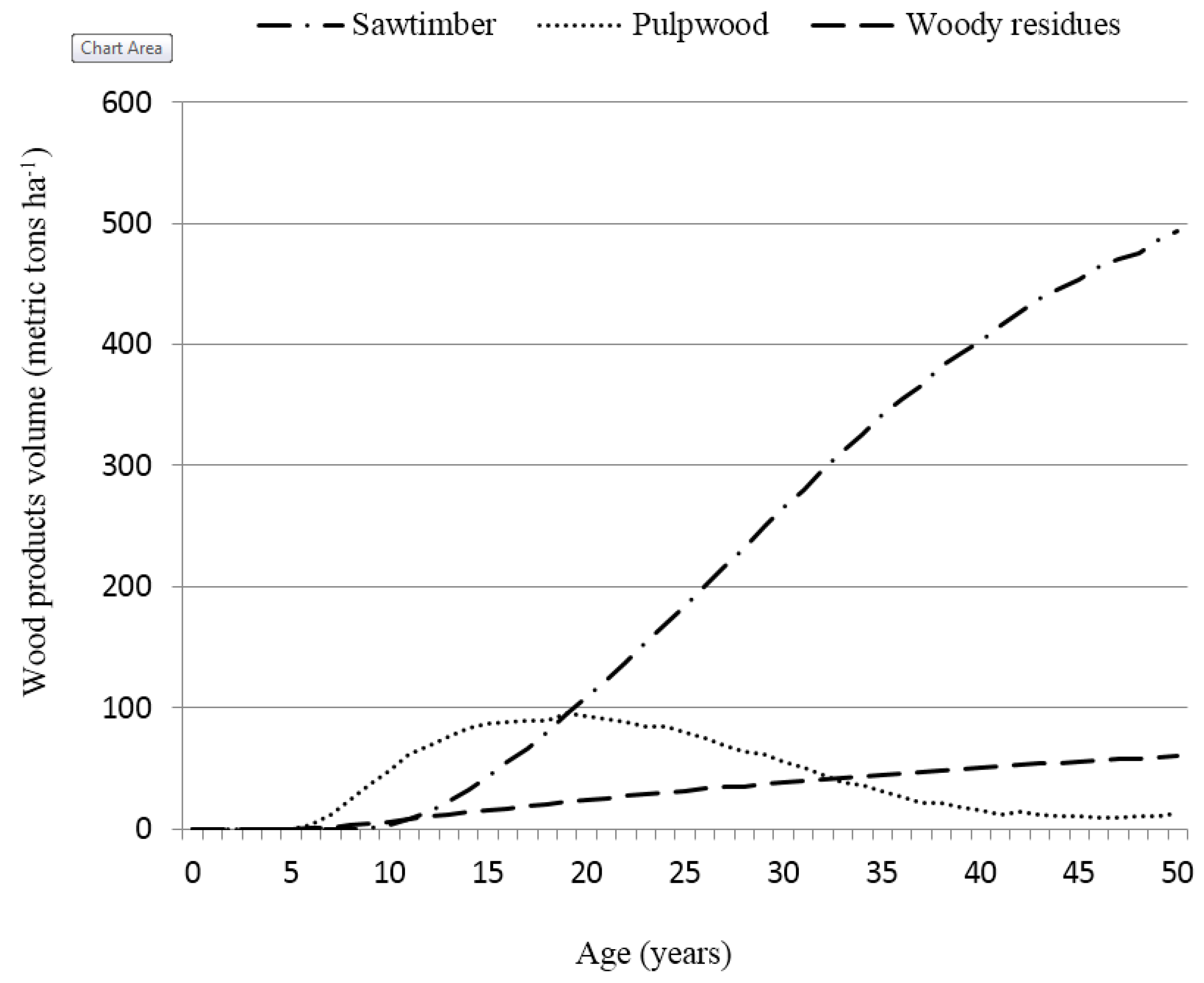
2.2. Growth and Yield Model

FASTLOB, a stand-level growth and yield model developed for management of loblolly pine plantations, was used to simulate growth and yield from stand age 0 to 50 years [29]. Both scenarios assume a planting density of 1235 trees ha⁻¹ and a site index of 18.3 m at age 25 years. The FASTLOB model assumed tree mortality that is typical of loblolly pine stands in the southeastern United States [29,30,31]. For fertilization, it was modeled that 168 kg·ha⁻¹ Nitrogen and 28 kg·ha⁻¹ of Phosphorus were applied when the stand was 12 years old. For thinning, every 3rd row was modeled to be removed at age 11 years. Annual output was obtained for trees ha⁻¹, basal area ha⁻¹, and volumes for sawtimber and pulpwood ha⁻¹. The volume of sawtimber was determined as the volume of sawtimber quality trees with a dbh equal to or greater than 19.1 cm up to a 15.2 cm inside bark diameter. The volume of pulp was determined as the volume up to a 10.2 cm outside bark top excluding the volume suitable for sawtimber. Volumes were converted to green metric tons using conversion factors obtained from Amateis et al. [29] and the quadratic mean dbh [32].

2.3. Amount of Wood for Bioenergy

It was assumed that the residue is sold as bioenergy feedstock for electricity production. Hence, the bioenergy (woody residue) is the amount left after subtracting the merchantable (sawtimber and pulpwood) volume from the total aboveground biomass. The total aboveground tree biomass was determined by multiplying the merchantable volume by the factor 1.1 [33]. The yield of timber products i.e., sawtimber, pulpwood, and bioenergy (metric tons) with respect to plantation age (years) is presented in Figure 1.

Figure 1. Amount of wood products—sawtimber, pulpwood, and woody residues (metric tons·ha⁻¹) with respect to plantation age (years).

Figure 1. Amount of wood products—sawtimber, pulpwood, and woody residues (metric tons·ha⁻¹) with respect to plantation age (years).

2.4. Amount of Carbon Sequestered and Emissions Saved from Bioenergy

The total aboveground tree biomass was multiplied by the factor β = 15.6 [34] to get the amount CO₂e stored in the standing volume of trees. Woody bioenergy (in the form of wood chips) obtained from harvest was assumed to displace coal for electricity production. The amount of CO₂e emissions offset from using bioenergy was calculated by multiplying the electricity generated (in kWh·ha⁻¹) from bioenergy by the factor 0.001236 Mg·CO₂e·kWh⁻¹ (1.2 kg·CO₂e·kWh⁻¹) [35], which is the GHG intensity of electricity generated from coal. The electricity generated from wood chips was calculated by multiplying the total availability of wood chips (Mg) with the calorific value of wood chips (12 MJ·kg⁻¹), conversion efficiency of a 100 megawatt (MW) power plant (31.7%) [36], and electricity transmission losses (7%) [37].

2.5. Amount of Carbon Emitted from Management and Harvesting

Assuming that slash pine and loblolly pine stands in the same region have similar management and harvesting regimes, data from Dwivedi et al. [23] was used to obtain the amount of CO₂e emissions from silvicultural operations. Thus, the amount of CO₂e emissions from site preparation and planting was taken as 1.1 Mg ha⁻¹, emissions from nitrogen and phosphorus fertilization application during age 12 years was taken as 3.031 Mg ha⁻¹, and emissions from machinery used during the harvesting operations was taken as 1.6 Mg ha⁻¹ [23].

2.6. Amount of Carbon Emitted from Decay of Wood Products

First, the amount of carbon remaining in each wood product (sawtimber and pulpwood) each year until 100 years after harvest was calculated using an exponential decay function as shown in Equation (1).

$$N_n=N_0\left(2^{\left(-n/hl\right)}\right)$$

(1)

where, N_n is the amount of CO₂e left after n years of harvest (Mg), N₀ is the amount of CO₂e left in the tree biomass at the time of harvest (Mg), n is the years after harvest (0 to 100 years), and hl is the half-life of each wood product (100 and 2.6 years respectively, for lumber derived from sawtimber and paper products derived from pulpwood [23]). Using Equation (1), the amount of CO₂e emitted from the decay of products each year after harvest through 100 years was determined using Equation (2).

$$C\left(n\right)=N_n-N_{\left(n-1\right)}$$

(2)

where, C(n) refers to the CO₂e emissions from the decay of sawtimber (or pulpwood) at year n (Mg), N_n is the amount of carbon left after n years of harvest (Mg), N_(n−1) is the amount of carbon left after (n − 1) years of harvest (Mg).

2.7. Economic Analysis

The Hartman model [25] was used to calculate the LEV and determine the optimal management regime for a loblolly pine plantation assuming carbon payments and bioenergy production. The forestland value is determined using Equation (3).

$$LEV\left(t\right)=\frac{pvc\left(t\right)+pvt\left(t\right)-pvm\left(t\right)}{1-e^{-rt}}$$

(3)

where, LEV(t) is the land expectation value at a time t assuming benefits from forests to be perpetual ($·ha⁻¹), pvc(t) is the net present value of carbon benefits ($·ha⁻¹), pvc(t) is the net present value of timber benefits ($·ha⁻¹), pvm(t) is the net present value of management cost over one rotation ($·ha⁻¹), t is the age of the stand that maximizes forest land value (years), and r is the real discount rate.

The net present value of the carbon benefits pvc(t) on a hectare of forestland over one rotation was calculated using Equation (4).

$$pvc\left(t\right)={\displaystyle \underset{0}{\overset{t}{\int }}{P}_c}{Q}_c\left(t\right)e^{-rt}dt+W_c\left(t\right)P_c{e}^{-rt}-P_c{Q}_f{e}^{-rt}-P_c{C}_m-{\displaystyle {\sum }_0^{100}{P}_{c}C\left(n\right)e^{-r\left(n+t\right)}}-P_c{H}_t{e}^{-rt}$$

(4)

where, P_c is the price of CO₂e ($·Mg⁻¹), Q_c(t) is the amount of CO₂e stored in tree biomass (Mg), W_c is the amount of CO₂e emission saved from using bioenergy for electricity production instead of coal (Mg), Q_f is the amount of CO₂e released from fertilization (Mg), C_m is the amount of CO₂e released during site preparation and planting (Mg), C(n) refers to the CO₂e emissions values from decay of sawtimber (or pulpwood) at year n (Mg), and H_t is the amount of CO₂e emitted during harvesting of stands (Mg).

Net present value of management cost pvm(t) on a hectare of forestland over one rotation is calculated using Equation (5).

$$pvm\left(t\right)={\displaystyle \underset{0}{\overset{t}{\int }}Y\left(t\right)}{e}^{-rt}dt+T_t{e}^{-rt}+F_t{e}^{-rt}+C_t$$

(5)

where, Y(t) is the yearly management cost ($·ha⁻¹), T_t is the marking cost for thinning ($·ha⁻¹), F_t is the fertilization cost ($·ha⁻¹), C_t is the site preparation and planting cost ($·ha⁻¹). Management costs were taken from Dwivedi et al. [23] and Fox et al. [38].

Net present value of the forest product harvest benefits pvt(t) over one rotation is determined using Equation (6).

$$pvt\left(t\right)=PQ\left(t\right)e^{-rt}$$

(6)

where, P is the vector of prices for sawtimber, pulpwood, and bioenergy ($·Mg⁻¹), and Q is the vector of volumes for sawtimber, pulpwood, and bioenergy. Stumpage prices were obtained from Timber Mart-South 2013 [39].

2.8. Sensitivity Analysis

A range of bioenergy, CO₂e, and forest product prices were analyzed. Three different stumpages prices for sawtimber and pulpwood reported in Timber Mart South 2013 [39] were used. The range of stumpage prices for sawtimber and pulpwood reflect the impact of different harvesting costs (e.g., fuel costs and topography), transportation distances, stand sizes, and other market variations. Finally, a range of CO₂e prices were examined—$0, $2, $5, $15, and $25 Mg⁻¹. This range of CO₂e prices is consistent with existing markets in the United States. For example, one of the regulatory markets in the United States, Regional Greenhouse Gas Initiative, has a clearing price of $3.1 Mg⁻¹ [40]. Similarly, another regulatory market, the California cap and trade program auctioned carbon permits at a price of $14.9 Mg⁻¹ [41]. The voluntary market, Mountain Association for Community Economic Development sells carbon offsets at prices $5.6 and $16.5 Mg⁻¹ for sale of at least one metric ton and larger sales of thousands of tons respectively [42]. Prices of $0 and $5 Mg⁻¹ were used for woody bioenergy based on the prices found in the literature [19,23].

3. Results and Discussion

Summary of the results for LEV calculations and optimal rotation age of the two management regimes under different carbon, bioenergy, and forest products (sawtimber and pulpwood) prices are shown in Table 1 and Table 2. The results show that in each of the management regimes at high, average, and low products prices, as expected, LEV increased with an increase of carbon and bioenergy prices. Carbon payments have a much larger impact on LEV than bioenergy. For example, in the thinning and fertilization scenario at average products prices, an increase in carbon price from $0 to $2 Mg⁻¹ increased LEV by $347.1 ha⁻¹ (at a bioenergy price of $0 Mg⁻¹), whereas increasing the bioenergy price from $0 to $5 Mg⁻¹ increased LEV by $66.3 ha⁻¹ (at a carbon price of $0 Mg⁻¹).

Table 1. Land expectation values (LEVs) at different bioenergy and carbon prices under three products prices and two management regimes in loblolly pine forests.

Bioenergy Price	CO2e Price	LEV ($ha−1)
		High Products Price *		Average Products Price **		Low Products Price ***
($Mg−1)	($Mg−1)	Thinning only	Thinning and fertilization	Thinning only	Thinning and fertilization	Thinning only	Thinning and fertilization
0	0	806.4	820.9	501.4	404.9	195.6	−10.5
	2	1034.8	1168.0	732.7	752.1	429.8	341.8
	5	1405.5	1688.7	1103.3	1278.5	800.5	874.6
	15	2689.3	3455.5	2407.3	3059.8	2124.9	2687.5
	25	4067.9	5262.8	3811.6	4891.9	3555.9	4520.2
5	0	848.7	888.9	543.7	471.3	237.9	54.4
	2	1075.7	1234.4	773.6	818.4	470.7	406.1
	5	1446.4	1755.0	1144.2	1342.8	841.4	936.9
	15	2726.0	3517.8	2444.1	3119.9	2161.4	2744.9
	25	4102.7	5319.5	3843.9	4948.6	3588.3	4576.9

*: High sawtimber and pulpwood prices, $28.2 Mg⁻¹ and $11.6 Mg⁻¹, respectively; **: Average sawtimber and pulpwood prices, $24.4 Mg⁻¹ and $9.6 Mg⁻¹, respectively; ***: Low sawtimber and pulpwood prices, $20.7 Mg⁻¹ and $7.6 Mg⁻¹, respectively.

Table 1. Land expectation values (LEVs) at different bioenergy and carbon prices under three products prices and two management regimes in loblolly pine forests.

Bioenergy Price	CO2e Price	LEV ($ha−1)
		High Products Price *		Average Products Price **		Low Products Price ***
($Mg−1)	($Mg−1)	Thinning only	Thinning and fertilization	Thinning only	Thinning and fertilization	Thinning only	Thinning and fertilization
0	0	806.4	820.9	501.4	404.9	195.6	−10.5
	2	1034.8	1168.0	732.7	752.1	429.8	341.8
	5	1405.5	1688.7	1103.3	1278.5	800.5	874.6
	15	2689.3	3455.5	2407.3	3059.8	2124.9	2687.5
	25	4067.9	5262.8	3811.6	4891.9	3555.9	4520.2
5	0	848.7	888.9	543.7	471.3	237.9	54.4
	2	1075.7	1234.4	773.6	818.4	470.7	406.1
	5	1446.4	1755.0	1144.2	1342.8	841.4	936.9
	15	2726.0	3517.8	2444.1	3119.9	2161.4	2744.9
	25	4102.7	5319.5	3843.9	4948.6	3588.3	4576.9

*: High sawtimber and pulpwood prices, $28.2 Mg⁻¹ and $11.6 Mg⁻¹, respectively; **: Average sawtimber and pulpwood prices, $24.4 Mg⁻¹ and $9.6 Mg⁻¹, respectively; ***: Low sawtimber and pulpwood prices, $20.7 Mg⁻¹ and $7.6 Mg⁻¹, respectively.

Table 2. Optimal Rotation Age at different bioenergy and carbon prices under three products prices and two management regimes in loblolly pine forests.

Bioenergy Price	CO2e Price	Optimal Rotation Age (Year)
		High Products Price *		Average Products Price **		Low Products Price ***
($Mg−1)	($Mg−1)	Thinning only	Thinning and fertilization	Thinning only	Thinning and fertilization	Thinning only	Thinning and fertilization
0	0	28	24	28	25	28	26
	2	31	25	31	25	31	26
	5	31	25	31	26	31	27
	15	36	27	36	28	37	30
	25	38	30	41	30	41	30
5	0	28	24	28	25	28	25
	2	31	25	31	25	31	26
	5	31	25	31	26	31	27
	15	36	27	36	28	36	30
	25	38	30	41	30	41	30

*: High sawtimber and pulpwood prices, $28.2 Mg⁻¹ and $11.6 Mg⁻¹, respectively; **: Average sawtimber and pulpwood prices, $24.4 Mg⁻¹ and $9.6 Mg⁻¹, respectively; ***: Low sawtimber and pulpwood prices, $20.7 Mg⁻¹ and $7.6 Mg⁻¹, respectively.

Table 2. Optimal Rotation Age at different bioenergy and carbon prices under three products prices and two management regimes in loblolly pine forests.

Bioenergy Price	CO2e Price	Optimal Rotation Age (Year)
		High Products Price *		Average Products Price **		Low Products Price ***
($Mg−1)	($Mg−1)	Thinning only	Thinning and fertilization	Thinning only	Thinning and fertilization	Thinning only	Thinning and fertilization
0	0	28	24	28	25	28	26
	2	31	25	31	25	31	26
	5	31	25	31	26	31	27
	15	36	27	36	28	37	30
	25	38	30	41	30	41	30
5	0	28	24	28	25	28	25
	2	31	25	31	25	31	26
	5	31	25	31	26	31	27
	15	36	27	36	28	36	30
	25	38	30	41	30	41	30

*: High sawtimber and pulpwood prices, $28.2 Mg⁻¹ and $11.6 Mg⁻¹, respectively; **: Average sawtimber and pulpwood prices, $24.4 Mg⁻¹ and $9.6 Mg⁻¹, respectively; ***: Low sawtimber and pulpwood prices, $20.7 Mg⁻¹ and $7.6 Mg⁻¹, respectively.

The results for optimal rotation age shows that in each of the two management scenarios at high, average, and low products prices, the increase in carbon payments increased the optimal rotation age. In contrast, the increase of bioenergy price has relatively little impact on optimal rotation age indicating that the impact of bioenergy markets on the product mix produced may not be substantial. For example, increasing the carbon prices from $0 to $25 Mg⁻¹ (at a bioenergy price of $0 Mg⁻¹) in the thinning only scenario, under average products prices, increased the rotation age by 13 years, whereas the optimal rotation age remained unchanged when the bioenergy price was increased from $0 to $5 Mg⁻¹ (at a carbon price of $0 Mg⁻¹).

3.1. Land Expectation Value by Products Prices and Management Regimes

As expected, the results indicate that the LEV for the thinning only scenario at all combinations of carbon and bioenergy prices considered is highest when the products prices are high, followed by average products prices and low products prices (Table 1) A similar trend was also observed in the thinning and fertilization scenario.

For the high products prices, the LEV in the thinning and fertilization scenario is higher than that in the thinning only scenario, at all combinations of carbon and bioenergy prices considered in the study (Table 1). For the average products prices, the LEV in the thinning only scenario is higher in two instances, one when there is no carbon offset and bioenergy payments, and the other when there is payments for the bioenergy ($5 Mg⁻¹) but no payments for carbon offsets. In all other combinations of carbon and bioenergy prices, the LEV is higher in the thinning and fertilization scenario. For the low products prices, the LEV in the thinning and fertilization scenario is higher only when the carbon price is above $2 Mg⁻¹ at both the bioenergy price of $0 and $5 Mg⁻¹. In general, the results indicate that at both bioenergy prices, as carbon prices increase the thinning only scenario becomes less optimal than the thinning and fertilization scenario. For example at a carbon price of $15 Mg⁻¹ and bioenergy price of $5 Mg⁻¹, the LEV in the thinning only scenario is $791.7, $675.9 and $582.8 ha⁻¹ less compared to the thinning and fertilization scenario for high, average, and low products prices, respectively. Similarly, at a zero carbon and bioenergy prices, the LEV in the thinning only scenario is $96.4 and $206.1 ha⁻¹ more than that in the thinning and fertilization scenario for average and low products prices, respectively, whereas, for high products price, the LEV in the thinning only scenario is $14.5 ha⁻¹ less than that in the thinning and fertilization scenario.

In the thinning only scenario there is no penalty for carbon emissions from fertilization use or cost associated with fertilization of the stands. Despite this, the LEV in this scenario is less than that in the thinning and fertilization scenario. This indicates that the benefits of increased growth from fertilization outweighed the penalty associated with emissions. For instance, for low products prices at the rotation age of 30 years, when the carbon price is $25 Mg⁻¹, the discounted carbon benefits for the thinning and fertilization scenario was $258.3 ha⁻¹ more than that for the thinning only scenario. At the same rotation age, the benefits from selling bioenergy at the price of $5 Mg⁻¹·yielded $44.1 and $41.0 ha⁻¹ for thinning and fertilization and thinning only scenarios respectively. Similarly, the benefits from using wood chips for electricity production instead of fossil fuels at the rotation age of 30 years and carbon price of $25 Mg⁻¹ for the thinning and fertilization scenario was $16.8 ha⁻¹ more than that of the thinning only scenario. The net present value of merchantable volume in the thinning and fertilization scenario was $116.5 ha⁻¹ more compared to the thinning only scenario.

In summary, the results show that the benefits of lower management costs and no carbon penalty from fertilization use in the thinning only scenario are outweighed by the benefits from carbon payments, bioenergy production, carbon offset benefits from using wood chips, and producing higher quantities of merchantable wood products in the thinning and fertilization scenario.

3.2. Optimal Rotation Age by Products Prices and Management Regimes

Optimal rotation ages for various carbon and bioenergy prices at high, average, and low products prices and the two management scenarios (thinning only and thinning and fertilization) are presented in Table 2. In the thinning only scenario under the high products prices, there is no change in the optimal rotation age as the bioenergy price is increased from zero to $5 Mg⁻¹ (keeping the carbon price the same). Similar is the case under the average products prices. For the low products prices, the optimal rotation age decreased by one year when the bioenergy price was increased to $5 Mg⁻¹ at constant carbon price of $15 Mg⁻¹. Similar is the trend in the thinning and fertilization scenario, with few exceptions at the high and low products prices. However, the decrease in the rotation age as a result of bioenergy benefits is negligible in both management scenarios and under all products prices considered.

In contrast, the increase in carbon prices increased the optimal rotation age in both management regimes under all the products prices. In the thinning only scenario, except at the higher prices of carbon ($15 to $25 Mg⁻¹) the optimal rotation age remained unchanged under high, average, and low products prices. In the thinning and fertilization scenario the optimal rotation age remained unchanged under all the products prices, at the carbon price of $25 Mg⁻¹. In all the other prices of carbon, the optimal rotation age increased up to 3 years as the products prices went from high to low. Within each of the products prices, with the increase of carbon price from zero to $25 Mg⁻¹, the optimal rotation age increased by about 13 years in the thinning only scenario and 5 years in the thinning and fertilization scenario. Comparing the optimal rotation age in both management scenarios, the thinning only scenario has a higher rotation age and has a much greater response to increased carbon prices compared to the thinning and fertilization scenario.

4. Conclusions

Based on the results, it can be concluded that including net carbon offset and woody bioenergy markets increase forest land values in both the thinning only and the thinning and fertilization scenarios under a range of sawtimber and pulpwood stumpage prices. This result is similar to the results obtained in other studies where net carbon payments and/or bioenergy production increase LEV [19,20,21,23,43]. We also found that carbon payments have a much larger impact on the LEV than bioenergy prices. The optimal choice between the thinning only and the thinning and fertilization scenario depends on the carbon offset prices, bioenergy prices, and products prices. For high products prices, at all the combination of carbon and bioenergy prices, the thinning and fertilization is the optimal management regime for the loblolly pine plantations in the southeastern United States. For average product prices, thinning only is the optimal management regime if there is no net carbon payments, whereas at all other combination carbon and bioenergy payments, the thinning and fertilization is the optimal choice. For the low products price, the optimal management regime depends on the combination of carbon and bioenergy prices. At a carbon price of $2 or less Mg⁻¹ and the bioenergy prices of either $0 or $5 Mg⁻¹, the thinning only is the optimal choice, at all the other combinations, the thinning and fertilization is the optimal management regime. These results suggest that carbon offset payments, bioenergy payments, and products prices may have a significant impact on the management regime chosen by landowners in the case of loblolly pine plantations.

An increase in the carbon price substantially increased the optimal rotation age. However, in contrast to some other studies [17,41,44], bioenergy payments did not decrease the optimal harvest age. This may indicate that bioenergy markets would not affect the stand level supply of traditional forest products. Similar results were found in a study by Snider and Cubbage [45], where the economic analysis showed that wood chip markets do not significantly shorten the optimal rotation age and the supply of sawtimber. Thus the impact of carbon and bioenergy markets on optimal rotation age and stand level supply of forest products varies depending on the forest type. It is important to note that the increase in LEV may increase the amount of land devoted to forest production and thus increase the supply of traditional forest products. This potential effect depends on the magnitude of the increase in LEV and the availability and alternative uses of land not used for forest production.

Several limitations of this study could be the focus of future work. This study assumed that 100% of the traditional wood products obtained at the time of harvest would be converted into various processed wood products. However, in practice, conversion of harvested wood products in the mills would generate residues such as bark, chunks, slabs, and sawdust depending upon the conversion efficiencies of the timber products. These mill residues can also be sold as bioenergy for electricity generation. For the forest carbon LCA, only carbon emissions associated with site preparation, management, and harvesting of forest stands were considered. Thus, there are other emission sources that could be studied such as carbon emissions associated with transportation, carbon recycled in various wood products, and carbon accumulated in landfills.

References

1. Miner, R.A.; Abt, R.C.; Bowyer, J.L.; Buford, M.A.; Malmsheimer, R.W.; O’Laughlin, J.; Oneil, E.E.; Sedjo, R.A.; Skog, K.E. Forest carbon accounting considerations in US bioenergy policy. J. For. 2014, 112, 591–606. [Google Scholar]
2. Ter-Mikaelian, M.T.; Colombo, S.J.; Chen, J. The burning question: Does forest bioenergy reduce carbon emissions? A review of common misconceptions about forest carbon accounting. J. For. 2015, 113, 57–68. [Google Scholar] [CrossRef]
3. Timmons, D.S.; Buchholz, T.; Veeneman, C.H. Forest biomass energy: Assessing atmospheric carbon impacts by discounting future carbon flows. GCB Bioenergy 2015. [Google Scholar] [CrossRef]
4. Hall, D.O.; Scrase, J.I. Will biomass be the environmentally friendly fuel of the future? Biomass Bioenergy 1998, 15, 357–367. [Google Scholar] [CrossRef]
5. Schubert, R. Future Bioenergy and Sustainable Land Use; Earthscan: Quicksilver Drive, Sterling, VA, USA, 2010. [Google Scholar]
6. Nepal, P.; Grala, R.K.; Grebner, D.L. Financial Feasibility of Sequestering Carbon for Loblolly Pine Stands in Interior Flatwoods Region in Mississippi. In Proceedings of the Southern Forest Economics Workers, Savannah, GA, USA, 9–11 March 2008; pp. 52–62.
7. Richards, K.R. A brief overview of carbon sequestration economics and policy. Environ. Manag. 2004, 33, 545–558. [Google Scholar] [CrossRef] [PubMed]
8. Sedjo, R.A. Forest Carbon Sequestration: Some Issues for Forest Investments; Resources for the Future: Washington, DC, USA, 2001. [Google Scholar]
9. Sedjo, R.A.; Sohngen, B.; Jagger, P. Carbon sinks in the post-Kyoto world. Clim. Chang. Econ. Policy Wash. DC. Resour. Futur. 2001, 134–142. [Google Scholar]
10. Shrum, T. Greenhouse Gas Emissions: Policy and Economics: A Report Prepared for the Kansas Energy Council Goals Committee; Kansas Energy Council: Topeka, KS, USA, 2007. [Google Scholar]
11. Gower, S.T. Patterns and mechanisms of the forest carbon cycle 1. Annu. Rev. Environ. Resour. 2003, 28, 169–204. [Google Scholar] [CrossRef]
12. White, M.K.; Gower, S.T.; Ahl, D.E. Life cycle inventories of roundwood production in northern Wisconsin: Inputs into an industrial forest carbon budget. For. Ecol. Manag. 2005, 219, 13–28. [Google Scholar] [CrossRef]
13. Skog, K.E.; Nicholson, G.A.; Joyce, L.A.; Birdsey, R. Carbon Sequestration in Wood and Paper Products; USDA, Forest Service, Rocky Mountain Research Station: Fort Collins, CO, USA, 2000. [Google Scholar]
14. Markewitz, D. Fossil fuel carbon emissions from silviculture: Impacts on net carbon sequestration in forests. For. Ecol. Manag. 2006, 236, 153–161. [Google Scholar] [CrossRef]
15. Johnson, L.R.; Lippke, B.; Marshall, J.D.; Comnick, J. Life-cycle impacts of forest resource activities in the Pacific northwest and southeast United States. Wood Fiber Sci. 2007, 37, 30–46. [Google Scholar]
16. Karjalainen, T.; Zimmer, B.; Berg, S.; Welling, J.; Schwaiger, H.; Finer, L.; Cortijo, P. Energy, Carbon and Other Material Flows in the Life Cycle Assessment of Forestry and Forest Products; European Forest Institute: Torikatu, Finland, 2001. [Google Scholar]
17. Catron, J.F.; Stainback, G.A.; Lhotka, J.M.; Stringer, J.; Hu, L. Financial and management implications of producing bioenergy in Upland Oak Stands in Kentucky. North. J. Appl. For. 2013, 30, 164–169. [Google Scholar] [CrossRef]
18. Susaeta, A.; Lal, P.; Alavalapati, J.; Mercer, E.; Carter, D. Economics of intercropping loblolly pine and switchgrass for bioenergy markets in the southeastern United States. Agrofor. Syst. 2012, 86, 287–298. [Google Scholar] [CrossRef]
19. Nesbit, T.S.; Alavalapati, J.R.R.; Dwivedi, P.; Marinescu, M.V. Economics of ethanol production using feedstock from slash pine (Pinus Elliottii) plantations in the southern United States. South. J. Appl. For. 2011, 35, 61–66. [Google Scholar]
20. Susaeta, A.; Alavalapati, J.R.R.; Carter, D.R. Modeling impacts of bioenergy markets on nonindustrial private forest management in the southeastern United States. Nat. Resour. Model. 2009, 22, 345–369. [Google Scholar] [CrossRef]
21. Stainback, G.A.; Alavalapati, J.R.R. Economic analysis of slash pine forest carbon sequestration in the southern US. J. For. Econ. 2002, 8, 105–117. [Google Scholar]
22. Van Kooten, G.C.; Binkley, C.S.; Delcourt, G. Effect of carbon taxes and subsidies on optimal forest rotation age and supply of carbon services. Am. J. Agric. Econ. 1995, 77, 365–374. [Google Scholar] [CrossRef]
23. Dwivedi, P.; Bailis, R.; Stainback, A.; Carter, D.R. Impact of payments for carbon sequestered in wood products and avoided carbon emissions on the profitability of NIPF landowners in the US South. Ecol. Econ. 2012, 78, 63–69. [Google Scholar] [CrossRef]
24. Dwivedi, P.; Alavalapati, J.R.R.; Susaeta, A.; Stainback, A. Impact of carbon value on the profitability of slash pine plantations in the southern United States: An integrated life cycle and faustmann analysis. Can. J. For. Res. 2009, 39, 990–1000. [Google Scholar] [CrossRef]
25. Hartman, R. The harvesting decision when a standing forest has value. Econ. Inq. 1976, 14, 52–58. [Google Scholar] [CrossRef]
26. Nix, S. Ten Most Common Trees in the United States. Available online: http://forestry.about.com/b/2012/07/21/ten-most-common-trees-in-the-united-states.htm (accessed on 24 January 2013).
27. Baker, J.B.; Langdon, O.G.  Pinus Taeda. In Silvics of North America; Burns, R.M., Honkala, B.H., Eds.; U.S. Department of Agriculture, Forest Service: Washington, DC, USA, 1990; pp. 497–512. [Google Scholar]
28. Eisenbies, M.H.; Vance, E.D.; Aust, W.M.; Seiler, J.R. Intensive utilization of harvest residues in southern pine plantations: Quantities available and implications for nutrient budgets and sustainable site productivity. Bioenergy Res. 2009, 2, 90–98. [Google Scholar] [CrossRef]
29. Amateis, R.L.; Burkhart, H.E.; Allen, H.L.; Montes, C. Fastlob: A Stand-Level Growth and Yield Model for Fertilized and Thinned Loblolly Pine Plantations; Computer Software: Blacksburg, VA, USA, 2001. [Google Scholar]
30. Amateis, R.L.; Burkhart, H.E.; Liu, J. Modeling survival in juvenile and mature loblolly pine plantations. For. Ecol. Manag. 1997, 90, 51–58. [Google Scholar] [CrossRef]
31. Pienaar, L.V.; Shiver, B.D. Survival functions for site-prepared slash pine plantations in the flatwoods of Georgia and northern Florida. South. J. Appl. For. 1981, 5, 59–62. [Google Scholar]
32. Curtis, R.O.; Marshall, D.D. Technical note: Why quadratic mean diameter? West. J. Appl. For. 2000, 15, 137–139. [Google Scholar]
33. Alabama Forestry Commission. Carbon Sequestration. Available online: http://www.forestry.state.al.us/CarbonSequestration.aspx?bv=5&s=0 (accessed on 11 June 2012).
34. Birdsey, R.A. Carbon storage for major forest types and regions in the conterminous United States. In Forests and Global Change; Sampson, R.N., Hair, D., Eds.; American Forests: Washington, DC, USA, 1996; Volume 2, pp. 1–25. [Google Scholar]
35. Lemoine, D.M.; Plevin, R.J.; Cohn, A.S.; Jones, A.D.; Brandt, A.R.; Vergara, S.E.; Kammen, D.M. The climate impacts of bioenergy systems depend on market and regulatory policy contexts. Environ. Sci. Technol. 2010, 44, 7347–7350. [Google Scholar] [CrossRef] [PubMed]
36. Bridgwater, A.V.; Toft, A.J.; Brammer, J.G. A Techno-economic comparison of power production by biomass fast pyrolysis with gasification and combustion. Renew. Sustain. Energy Rev. 2002, 6, 181–246. [Google Scholar] [CrossRef]
37. Energy Information Administration. How much Electricity Is Lost in Transmission and Distribution in the United States? United States Energy Information Administration: Washington, DC, USA, 2012. Available online: http://www.eia.gov/tools/faqs/faq.cfm?id=105&t=3 (accessed on 13 January 2013).
38. Fox, T.R.; Allen, H.L.; Albaugh, T.J.; Rubilar, R.; Carlson, C.A. Tree nutrition and forest fertilization of pine plantations in the southern United States. South. J. Appl. For. 2007, 31, 5–11. [Google Scholar]
39. Timber Mart-South. In Market News Quarterly: 4th Quarter 2014; Center for Forest Business, Warnell School of Forestry and Natural Resources, Frank W. Norris Foundation: Athens, GA, USA, 2014.
40. Potomac Economics. In Market Monitor Report for Auction 19; Regional Greenhouse Gas Initiative: New York, NY, USA, 2013.
41. Point Carbon. CCAs Rise 6 Percent on Strong Auction Results; A Point Carbon News; Carbon Market North America. 2013. Available online: http://www.pointcarbon.com/news/1.2202575 (accessed on 28 March 2013).
42. Shouse, S.; Mountain Association for Community Economic Development, Berea, KY, USA. Personal communication, 12 February 2013.
43. Shrestha, P.; Stainback, G.A.; Dwivedi, P.; Lhotka, J.M. Economic and life-cycle analysis of forest carbon sequestration and wood-based bioenergy offsets in the central hardwood forest region of United States. J. Sustain. For. 2015, 34, 214–232. [Google Scholar] [CrossRef]
44. Schaberg, R.H.; Aruna, P.B.; Cubbage, F.W.; Hess, G.R.; Abt, R.C.; Richter, D.D.; Warren, S.T.; Gregory, J.D.; Snider, A.G.; Sherling, S. Economic and ecological impacts of wood chip production in north Carolina: An integrated assessment and subsequent applications. For. Policy Econ. 2005, 7, 157–174. [Google Scholar] [CrossRef]
45. Snider, A.G.; Cubbage, F.W. Economic analyses of wood chip mill expansion in north Carolina: Implications for Nonindustrial Private Forest (NIPF) management. South. J. Appl. For. 2006, 30, 102–108. [Google Scholar]