
A Synthetic Landscape Metric to Evaluate Urban Vegetation Quality: A Case of Fuzhou City in China
by
Xisheng Hu
1, 
Chongmin Xu
1,
Jin Chen
1,
Yuying Lin
2,*,
Sen Lin
1,
Zhilong Wu
1 and
Rongzu Qiu
1 1
College of Transportation and Civil Engineering, Fujian Agriculture and Forestry University, Fuzhou 350002, China
2
College of Tourism, Fujian Normal University, Fuzhou 350108, China
*
Author to whom correspondence should be addressed.
Forests 2022, 13(7), 1002; https://doi.org/10.3390/f13071002
Submission received: 30 May 2022
/
Revised: 21 June 2022
/
Accepted: 23 June 2022
/
Published: 25 June 2022
(This article belongs to the Section Urban Forestry)
Abstract
:Urban vegetation plays a very important role in regulating urban climate and improving the urban environment. There is an urgent need to construct an effective index to quickly detect urban vegetation quality changes. In this study, a synthetic vegetation quality index (VQI) was proposed using a holistic approach based on the quality of vegetation itself and the spatial relationship with its surroundings, composed of four selected variables: normalized difference vegetation index (NDVI), patch aggregation index (AI), patch density (PD), and percentage of landscape (PLAND). Principal component analysis (PCA) was employed to calculate weights for each variable due to its objectivity. Then, taking Fuzhou City, southeast China as the case study, the scale effects of the VQI under different moving window sizes (500 m, 1 km, 2 km, …, 5 km) and the spatiotemporal changes were explored. The results showed that a VQI with a window size of 3 km had the highest correlations with all the selected indicators. Meanwhile, the representativeness and the effectiveness of the VQI were validated by the percentage eigenvalues of PC1, as well as Pearson correlation analysis and bivariate spatial autocorrelation analysis. We also revealed that the proposed VQI had the greatest explanatory power for land surface temperature (LST) among all the factors in both studied years (2000 and 2016), with the VQI’s interpretation of LST being 0–44% better than any individual indicator except for AI in 2000. Additionally, our work revealed that the location of vegetation has a great impact on the urban thermal environment. The VQI can assess urban vegetation quality effectively and quickly.
1. Introduction
Global urban area increased from 362,700 km2 in 1985 to 653,400 km2 in 2015, with a net growth rate of up to 80% [1], and it is projected to increase by 1.2 million km2 by 2030, which is nearly three times the area in 2000 [2]. Although urbanization has significantly promoted socioeconomic welfare for urban residents, this process can potentially threaten a broad array of ecosystem services [3,4]. As a consequence, experts in different research fields are constantly striving to seek countermeasures for sustainable urban development [5]. Urban vegetation, which is an important indicator to measure urban forest vegetation coverage, determined by plant species, growth status, coverage density, and spatial pattern context, can provide a variety of ecosystem services for urban dwellers [6,7,8]. Higher vegetation coverage has always been considered to have a greater mitigation effect on the urban heat environment with a higher shading canopy and evapotranspiration rate [9]. However, land resources are very scarce in densely populated urban areas, motivating research to optimize the spatial layout of vegetation coverage to mitigate urban eco-environmental problems. In this context, it is a prerequisite to develop an appropriate quantitative index to assess the quality of urban vegetation for rational planning and construction of urban vegetation.
Many indices have been proposed to estimate urban vegetation status, including plot-based and remote sensing-based measures. Plot-based index estimates from field measurements, including diameter at breast height, height of tree, crown size, and plant species, have been used to investigate species diversity, stand density, basal volume, biomass, etc. [10,11]. However, plot-based data collection is a labor-intensive task, leading to a relatively limited study scope and coarse-spatial-resolution data [6]. With the advancement of remote sensing technology, its utilization to detect vegetation dynamics, including quality and quantity, has blossomed quickly in recent years [10]. Remote sensing has not only been employed to identify vegetation area and extents, but also to quantify biophysical features of trees or forests [12]. The normalized difference vegetation index (NDVI) is one of the critical parameters reflecting the growth and nutritional information of vegetation, which has been extensively employed to assess eco-environmental changes [13]. NDVI is commonly defined as the ratio of the difference between the reflection value of the near-infrared band and the reflection value of the red band to their sum in remote sensing images [14]. NDVI has important implications for urban energy balance, air purification, climate regulation, and providing recreational venues for humans [7,15,16]. In urban areas, the leaf area index (LAI) is another simple and promising optically ecological index to monitor vegetation growth dynamics, which can be measured using plot data, light detection and ranging (LiDAR) data, or both [17]. Above-ground biomass has been quantified by radar images, such as Radarsat, ALOS Palsar, Sentinel 1, and LiDAR [18,19,20].
One of the challenges in assessing vegetation quality is that there is still a lack of a unified standard definition for vegetation quality. Some previous studies used a single indicator (e.g., NDVI or LAI) to estimate vegetation quality, while others used several indicators (e.g., basal area and volume) [10]. However, few studies have constructed a comprehensive index to evaluate vegetation quality. Several studies attempted to detect urban ecological change using a remote sensing-based ecological index (RSEI), composed of a couple of indicators integrated via principal component analysis (PCA) [21,22]. Some previous studies also employed PCA to develop synthetic landscape indices to observe the cooling effect of urban vegetation [23]. Unfortunately, most previous studies evaluated the quality of urban vegetation from an individual perspective and ignored the impact of the surrounding landscape. Therefore, the construction of a comprehensive index considering the spatial correlation of urban vegetation merits further study.
In this context, this study aimed to construct a comprehensive index to evaluate urban vegetation quality, considering both the quality of the vegetation and its spatial relationship with the surroundings, via the utilization of geospatial technology. This index is spatially explicit; specifically, it can be spatially visualized at the pixel level, which allows it to quickly, quantitatively, and objectively evaluate the regional vegetation quality.
2. Materials and Methods
2.1. Study Area
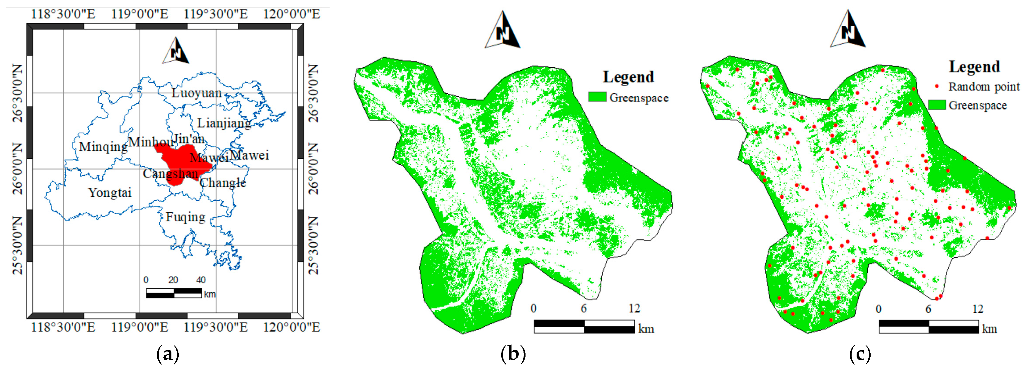
Fuzhou City is the capital of Fujian Province and one of the central cities in the economic zone on the west side of the Taiwan Straits. The total area is 11,968 km2, and the built-up area is 416 km2. Fuzhou has a typical subtropical monsoon climate, with moderate temperatures; it is warm, humid, and evergreen throughout the year, with plenty of sunshine, abundant rainfall, little frost and no snow, long summers, and short winters, characterized by a frost-free period of 326 days in a year. The annual average sunshine is 1700–1980 h, the annual average precipitation is 900–2100 mm, and the annual average temperature is 20–25 °C; the coldest month is January/February, with an average temperature of 6–10 °C, whereas the hottest month is July/August, with an average temperature of 33–37 °C. The maximum extreme temperature is 42.3 °C and the lowest is −2.5 °C. According to the seventh census data, the population of Fuzhou City was 829 million in 2020. Fuzhou achieved a GDP of 1002.02 billion CNY in 2020, a 5.1% increase compared to the previous year. In this study, we focused on the highly urbanized areas of the city (i.e., the red areas in Figure 1a). The study area was the central urban area, covering approximately 660.546 km2. This selected area experienced extremely rapid urbanization in the past 20 years, becoming one of the new furnace cities in China, with the annual high temperature duration ranking among the highest in the country [21]. Consequently, a study on the spatiotemporal variation in the vegetation quality of this area is meaningful, and it can also be applied to rapidly urbanized cities in other regions.
2.2. Data Source and Preprocessing
Two cloud-free Landsat-7 and Landsat-8 images with a spatial resolution of 30 m acquired on 4 May 2000 and 25 June 2016 were employed to extract the greenspace. The two images were obtained from the United States Geological Survey (USGS) (https://glovis.usgs.gov/) (accessed on 3 September 2020). The extraction of greenspace was accomplished in five steps: (1) the digital number (DN) of the multi-spectral bands was converted to the radiation brightness using the radiometric calibration tool in the ENVI software; (2) the atmospheric correction was processed using the FLAASH tool of the ENVI; (3) the normalized difference vegetation index (NDVI) was calculated according to (NIR − red)/(NIR + red); (4) the greenspace of the two studied years was extracted using the artificial threshold method, with threshold values of 0.52 for 2000 and 0.48 for 2016; (5) visual interpretation by comparing high-resolution Google images was employed to verify the classification accuracy using a confusion matrix with 100 random points for 2016 (Figure 1c). The accuracy was not verified for the year 2000 because the corresponding high-resolution image was unavailable. The overall classification accuracy of the greenspace in 2016 was 87.0%, and the kappa coefficient was 0.824. The land surface temperature (LST) was retrieved using the single-channel algorithm [24,25]. The inversion results of the LST were verified by correlation analysis, and the results showed that the correlations with the indices of the NDVI, land surface moisture, and normalized differential built-up and soil index were between 0.956 and 0.993 for both years, highlighting the reliability of the inversion results [24].
2.3. Calculation of Urban Vegetation Quality Index
2.3.1. Selection of Representative Metrics
To overcome the limitations of small-scale empirical indices and the neglection of spatial teleconnections of homogeneous plaques, landscape metrics, quantifying the spatial characteristics of patches, classes of patches, or entire landscape mosaics, have been developed on the basis of graph theory [26] to examine the changes in vegetation patterns [5,27,28,29]. These metrics can be divided into two general categories: those quantifying landscape composition without spatial attributes, and those quantifying the spatial configuration of the landscape in a spatial context [30]. Landscape composition refers to the magnitude and proportion of each patch type or the diversity and abundance of patch types within a study region, regardless of their spatial pattern, such as placement or location of patches within a mosaic [30], e.g., the percentage of a certain landscape element (PLAND) and the patch density (PD). Spatial configuration refers to the spatial pattern of patches, such as the spatial arrangement, location, or orientation of patches within a landscape. For example, patch division or patch aggregation (AI) measures the placement of patches relative to other patches, whereas the landscape shape index (LSI), fractal dimension index (FRAC), and edge density (ED) measure the spatial characteristics of the patches. Such metrics represent the recognition of a patch type according to its ecological properties, which are influenced by their shape and size, as well as their surroundings.
Screening representative landscape metrics is essential for a specific study area to construct the vegetation quality index (VQI). The principles of selecting landscape metrics in this study are comprehensiveness, interpretability, and ecological significance [5,31,32]. Consequently, a total of six metrics at the class level were considered, including the commonly used composition metrics, PLAND and PD, and the commonly used spatial configuration metrics, LSI, FRAC, ED, and AI. These class metrics were calculated using a moving window strategy. Briefly, each calculated grid (i.e., 30 m) of the study area yields a parameter value, with the consideration of all its defined neighboring cells in the square window, and, by moving the window, all grids of the study area are assigned a value (i.e., the abovementioned metrics). To compare the scale effect and obtain the optimized results, several window sizes were designed to calculate the class metrics using the Fragstats software, namely, 500 m × 500 m, 1 km × 1 km, 2 km × 2 km, 3 km × 3 km, 4 km × 4 km, and 5 km × 5 km. This software has a detailed operation guide [30], including formulas and parameter settings. Therefore, the calculation formula is not repeated here. Because the study area was an urban center area, the spatial distribution of the greenspace was discontinuous. If the moving window is too small, there will be many pixels with no value in the class metrics of the green space; if the moving window is too large, the spatial variation of the type index of green space will be too smooth. After careful comparison of the calculation results, it was decided to use a moving window size of 3 km as the calculation window for this study.
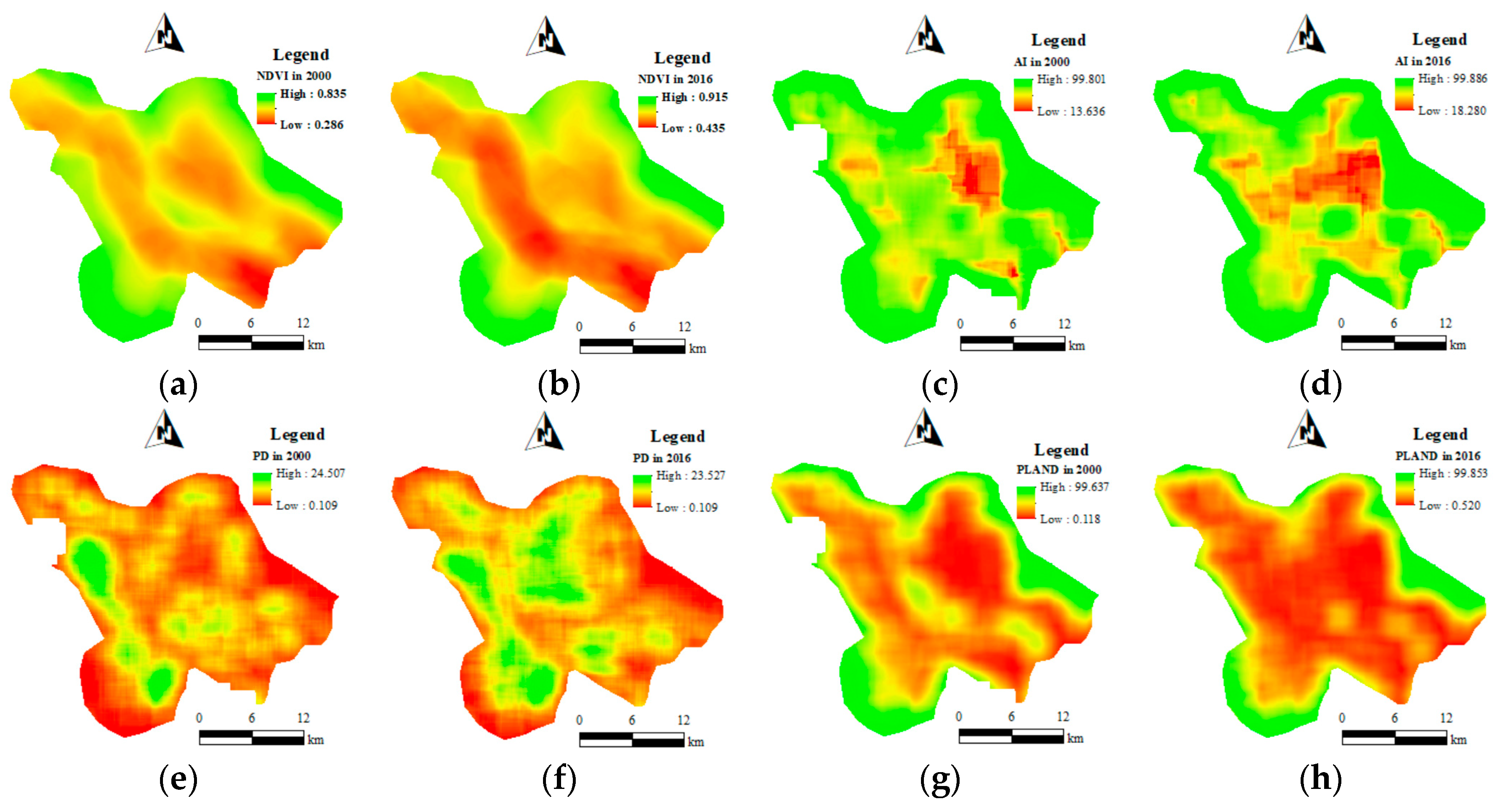
The calculation results showed that the indices related to the shape of greenspace patches (i.e., ED, LSI, and FRAC) were not sensitive across the study area, with their values hardly changing across the entire study area. Finally, the three-landscape metrics were selected (Figure 2 and Table 1): (1) AI, in the range of 0–100, examining the connectivity between greenspace patches, where a smaller value indicates a more discrete greenspace; (2) PD, in the range of 0–100, describing the degree of landscape fragmentation, where a larger value indicates a more shattered greenspace; (3) PLAND, in the range of 0–100, reflecting the percentage of greenspace. These three metrics are the most intuitive and frequently used class metrics [31,33]. Therefore, they were considered to be representative of the study area.
2.3.2. Construction and Testing of Urban Vegetation Quality Index
On the basis of the above-calculated landscape metrics, representing the amount and spatial configuration of the greenspace, combined with NDVI, indicating the quality of the greenspace, the proposed VQI was integrated using four metrics, AI, PD, PLAND, and NDVI. Then, the weight for each variable was determined to construct the VQI index. At present, there are many potential weighting methods, such as the commonly used analytic hierarchy process (AHP) and the Delphi method. However, these methods rely on expert experience and are highly subjective. In this study, we used PCA to compute the weight of each variable [21,24,34]. PCA is a compression method for multidimensional data, which can remove the multicollinearity between variables [35]. More importantly, the weight of each variable is automatically and objectively allocated according to its respective contribution to the principal components, which can eliminate the subjectivity of artificially determining weights. The PCA rotation tool was employed to process the PCA in ENVI; thus, the first PC (PC1) was used to build the VQI images for the both years.
In this study, the moving window strategy, percentage eigenvalue, Pearson correlation matrix, and bivariate spatial autocorrelation analysis were employed to test the robustness of the VQI. We applied a “moving window” strategy to compute the landscape metrics across the study area, which allowed us to filter the optimized results in terms of the percentage eigenvalue. PCA is a statistical method, which transforms a set of potentially correlated variables (e.g., four indicators in this case) into a group of linearly uncorrelated variables through orthogonal transformation, namely, PCs. PC1 is then employed to represent a new comprehensive index, under the premise of it accounting for a large variance, thus representing more information from the original variables. The variance is usually measured by the correlation between indicators and the percentage eigenvalue. The correlation coefficient ranges between −1 and 1, with closer absolute values to 1 being better; the percentage eigenvalue ranges between 0% and 100%, with larger values being better. Furthermore, we used Pearson correlation analysis and bivariate spatial autocorrelation analysis to analyze the correlation between the proposed VQI and each factor. A larger index (i.e., R2 and Moran’s I) indicates stronger explanatory power of the proposed VQI for each factor. Pearson correlation analysis and bivariate spatial autocorrelation analysis were carried out using the Statistical Program for Social Sciences (SPSS) (IBM) and Geoda software (https://geodacenter.github.io/download.html) (accessed on 1 December 2020), respectively.
3. Results
3.1. Scale Effects of the Synthetic Vegetation Quality Index
3.1.1. Correlations between VQI Indicators
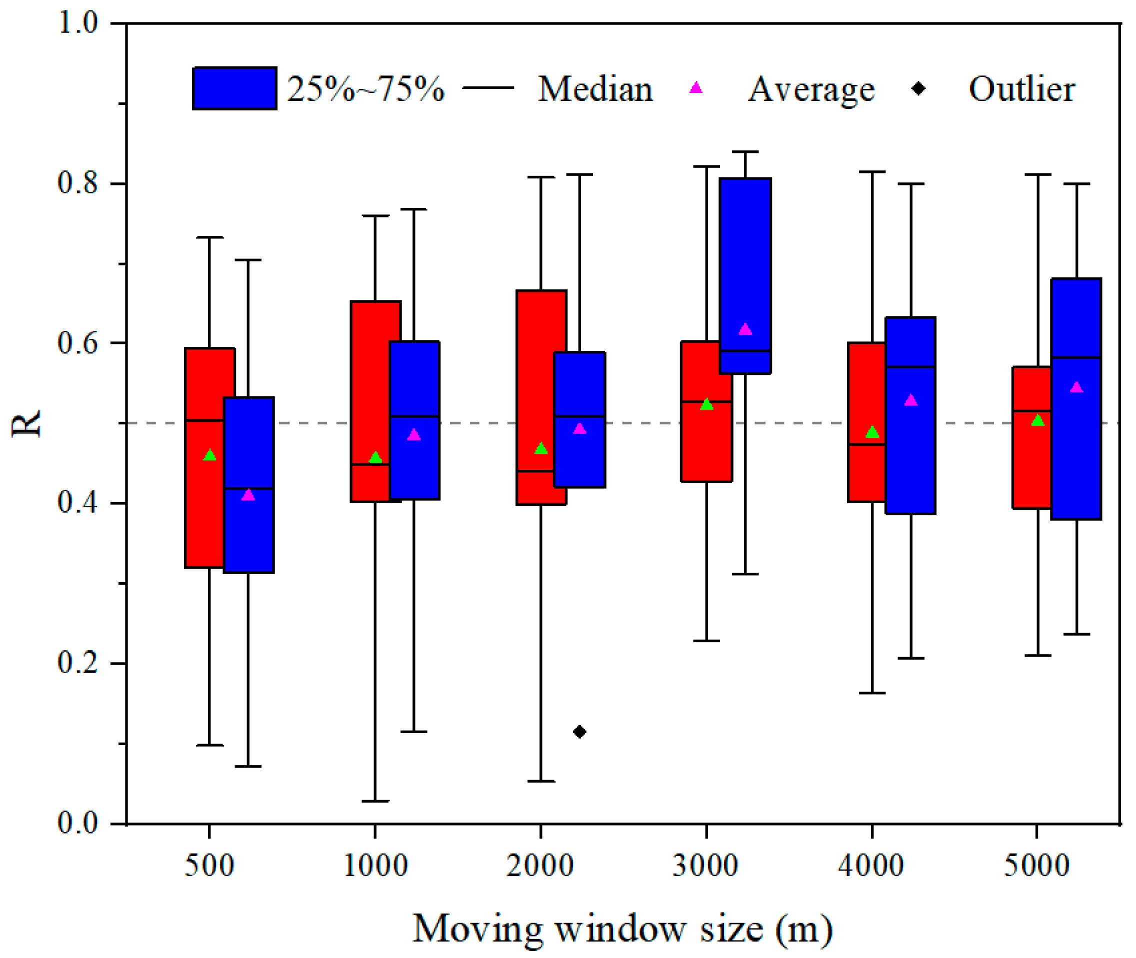
Table 2 indicates that all the indicators of VQI were highly correlated and statistically significant at the 1% level for all window sizes, except for the relationship between PD and NDVI for a window size of 1 km, which was statistically significant at the 5% level. Specifically, PD was consistently negatively correlated with the other indicators (i.e., PLAND, AI, and NDVI) for all window sizes, while all the other factors were positively correlated. Among all the factor pairs, the correlation between PLAND and AI was the highest, with a correlation coefficient of 0.706–0.822, while the correlation between NDVI and PD was the lowest, with a correlation coefficient between −0.029 and −0.312. Moreover, it should be noted that among all window sizes, the average correlation coefficient of 3000 m was the largest in both 2000 and 2016, with values of 0.523 and 0.618, respectively (Figure 3).
3.1.2. Principal Component Analysis
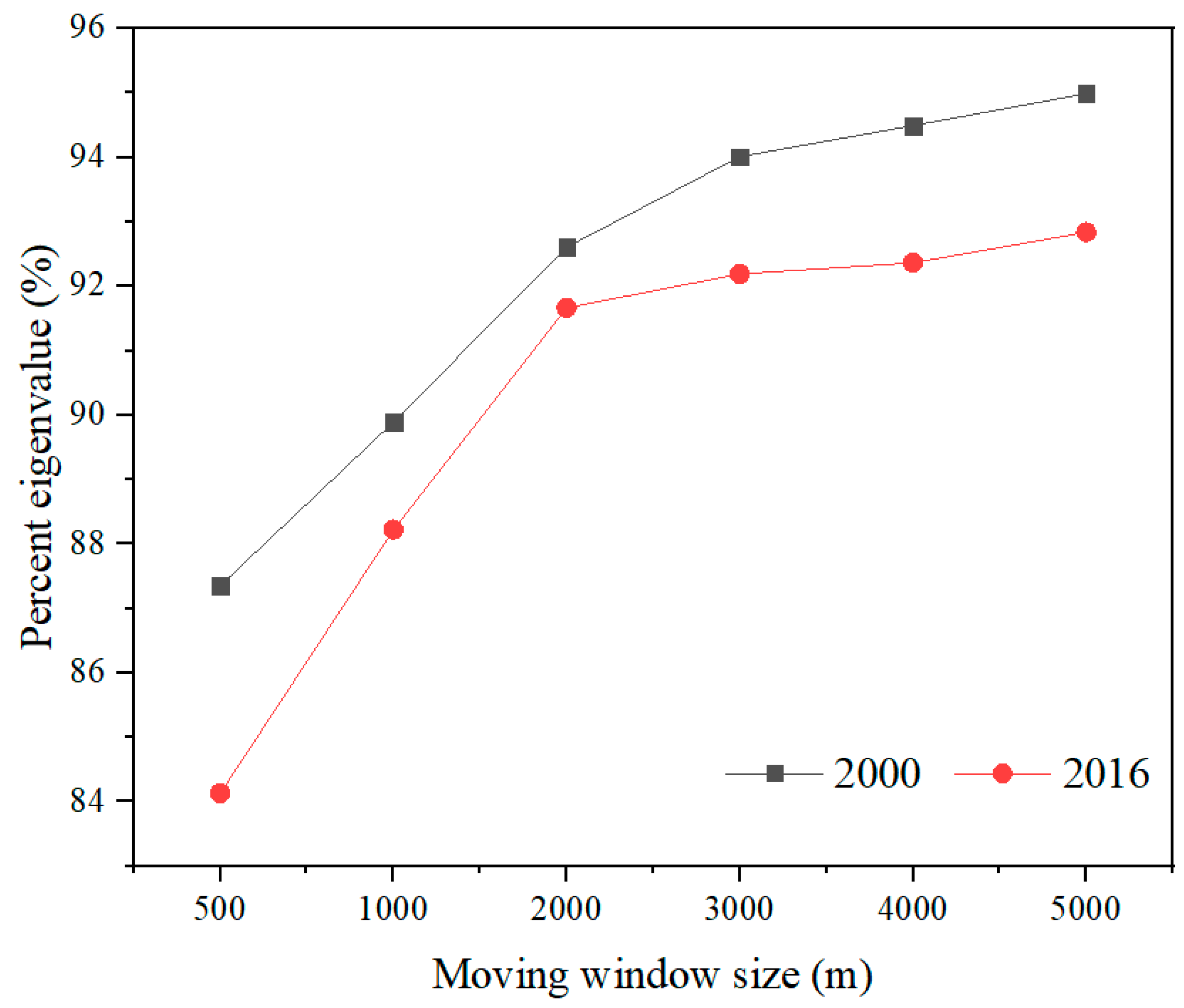
Table 3 shows the PCA results of VQI, indicating that the percentage eigenvalues of PC1 were 84.134–94.993% for all window sizes in both of the studied years. Figure 4 reveals that the percentage eigenvalues increased as the window size increased, with the curves growing quickly up to a window size of 3 km before becoming relatively stable in both of the studied years. The percentage eigenvalues of PC1 were 94.014% and 92.192% for a window size of 3 km in 2000 and 2016, respectively, indicating that this component could express more than 92% of the information of all the factors. The correlations among all VQI indicators were also highest for a window size of 3 km; thus, PC1 with a 3 km window size was chosen to construct the VQI.
3.2. Validity of the Synthetic Vegetation Quality Index
Pearson correlation analysis and bivariate spatial autocorrelation analysis revealed that the VQI and all its indicators were significantly correlated (p < 0.01) (Table 4). Among all the indicators, the VQI had the highest correlation with PLAND, with a correlation coefficient as high as 0.952–0.996, while the correlation between the VQI and PD was the lowest, with a correlation coefficient between −0.440 and −0.589. The average correlation coefficient values between the VQI and the other indicators were 0.76–0.82.
According to Pearson correlation analysis, the average coefficients between the VQI and each variable were 0.793 and 0.820 in 2000 and 2016, respectively, higher than those of any other factor pairs (Table 4).
Additionally, Pearson correlation and bivariate spatial autocorrelation were adopted to compute the correlations between the VQI and LST at the pixel level (30 m) (Table 5). Both the coefficients of Pearson correlation and Moran’s I of bivariate spatial autocorrelation demonstrated that all the indicators were significantly related to LST except for NDVI in 2000. Specifically, the influence of PD was consistently positive and statistically significant at the 1% level in both studied years, while the effects of other variables were consistently negative and statistically significant at the 1% level (except for NDVI in 2000 for the spatial autocorrelation analysis) in both studied years. As expected, the VQI had the greatest correlation with LST among all the factors in both studied years except for AI in 2000, indicating that the VQI’s interpretation of LST was 0–44% better than that of any other indicators in both studied years except for AI in 2000. Moreover, AI also had a higher potential explanatory power for LST, closely followed by PLAND. However, the exception was that NDVI was not highly correlated with LST, with correlation coefficients between −0.121 and −0.011.
3.3. Spatiotemporal Characteristics of Vegetation Quality
Figure 5 reflects the distribution patterns of the VQI using histograms generated individually for each VQI with an interval of 10 in 2000 and 2016, where the lines are the kernel smooth curves of the VQI, denoting the frequency estimation with kernel functions. Figure 6 illustrates that the degree of right-skewed distribution of the VQI in 2016 was greater than that in 2000, with skewness values of 0.720 for 2016 and 0.415 for 2000. These figures also demonstrated that the location of the maximum bin shifted to the left from 2000 to 2016. The maximum bin for 2000 was in the range of 40–50, while that for 2016 was in the range of 30–40.
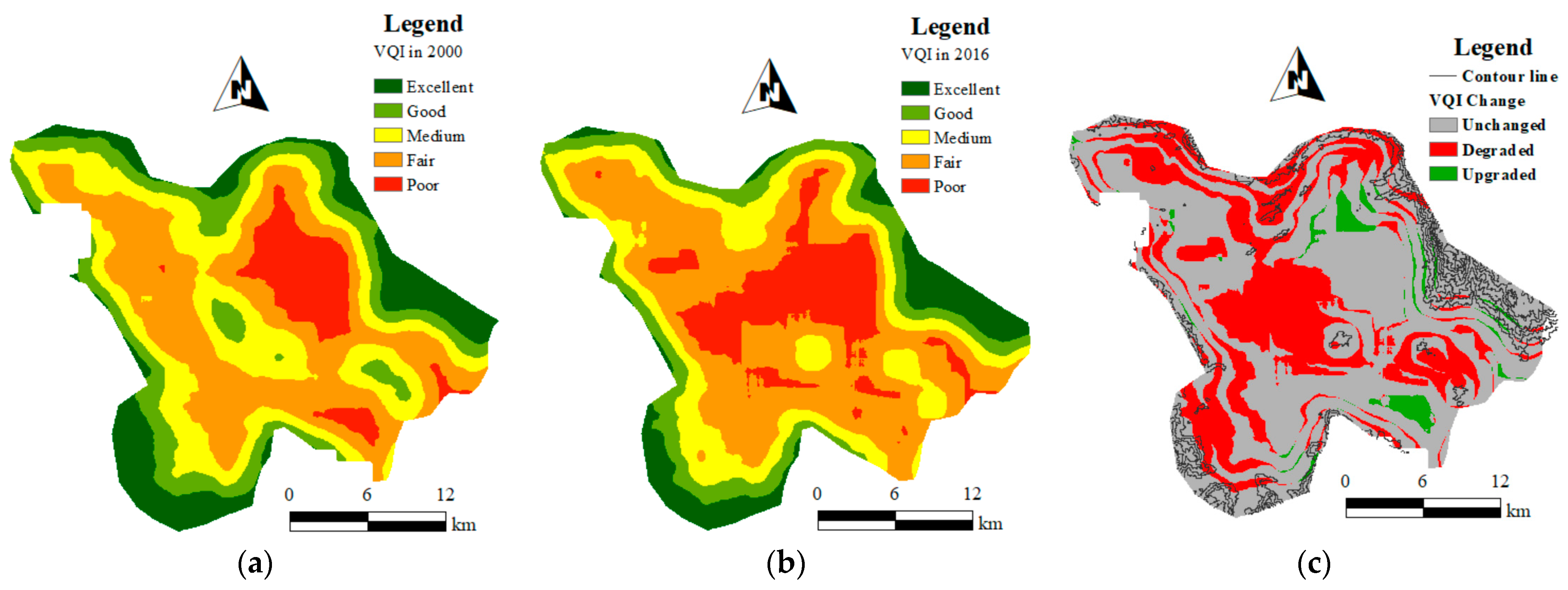
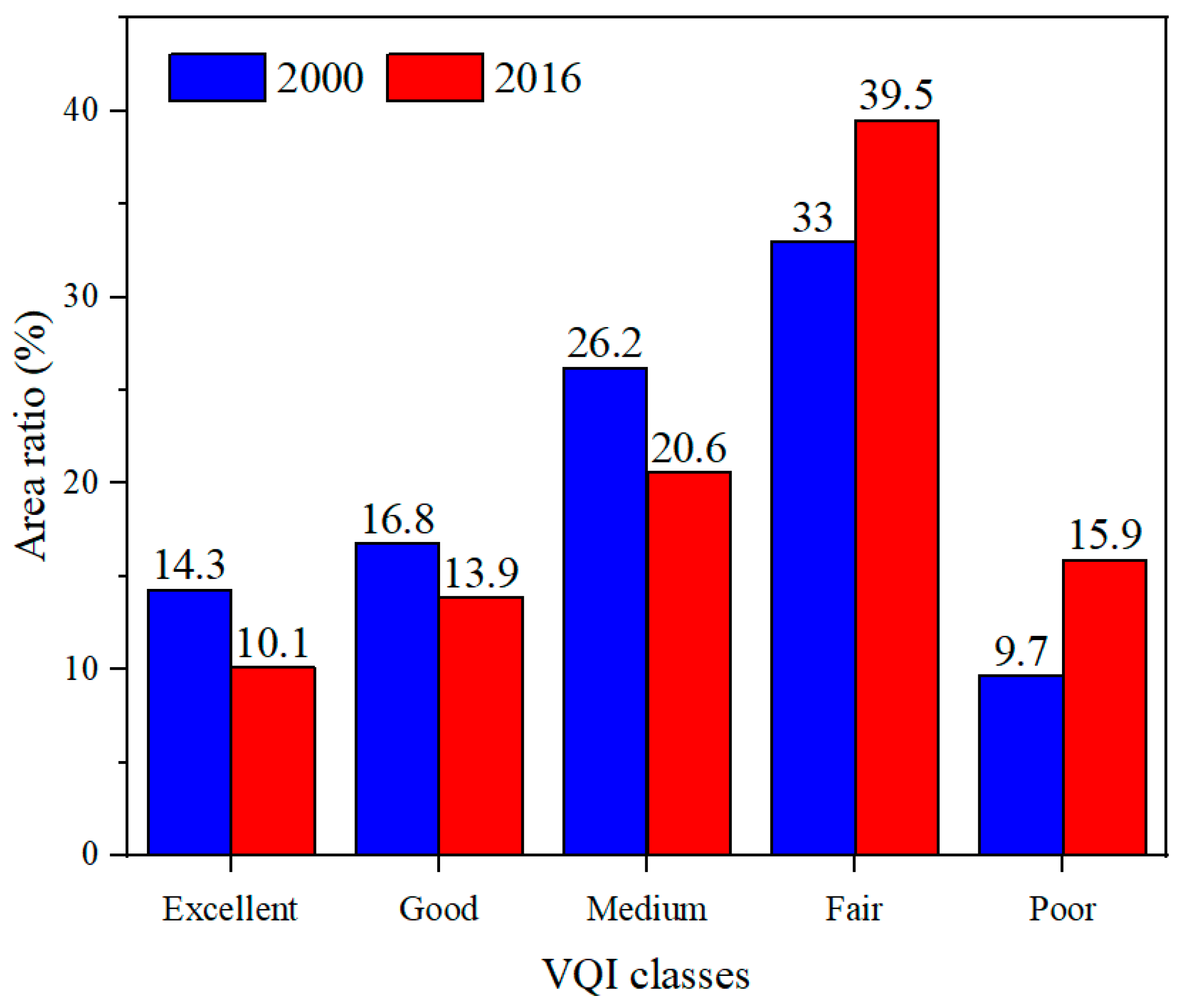
To facilitate the analysis of the spatiotemporal variations in the VQI, the VQI initial values were standardized within the range of 0–1, where a closer value to 1 indicates a higher vegetation quality, and vice versa. Then, the standardized RSEI was classified into five levels using the natural break (Jenks) method (Figure 6 and Figure 7): excellent, good, moderate, fair, and poor. Table 1 shows that the VQI decreased slightly from 0.492 in 2000 to 0.424 in 2016. Figure 7 reveals that the excellent level of the VQI decreased from 14.3% in 2000 to 10.1% in 2016, and the good level of the VQI also decreased from 16.8% in 2000 to 13.9% in 2016, while the fair and poor levels of the VQI increased from 33.0% and 9.7% in 2000 to 39.5% and 15.9% in 2016, respectively.
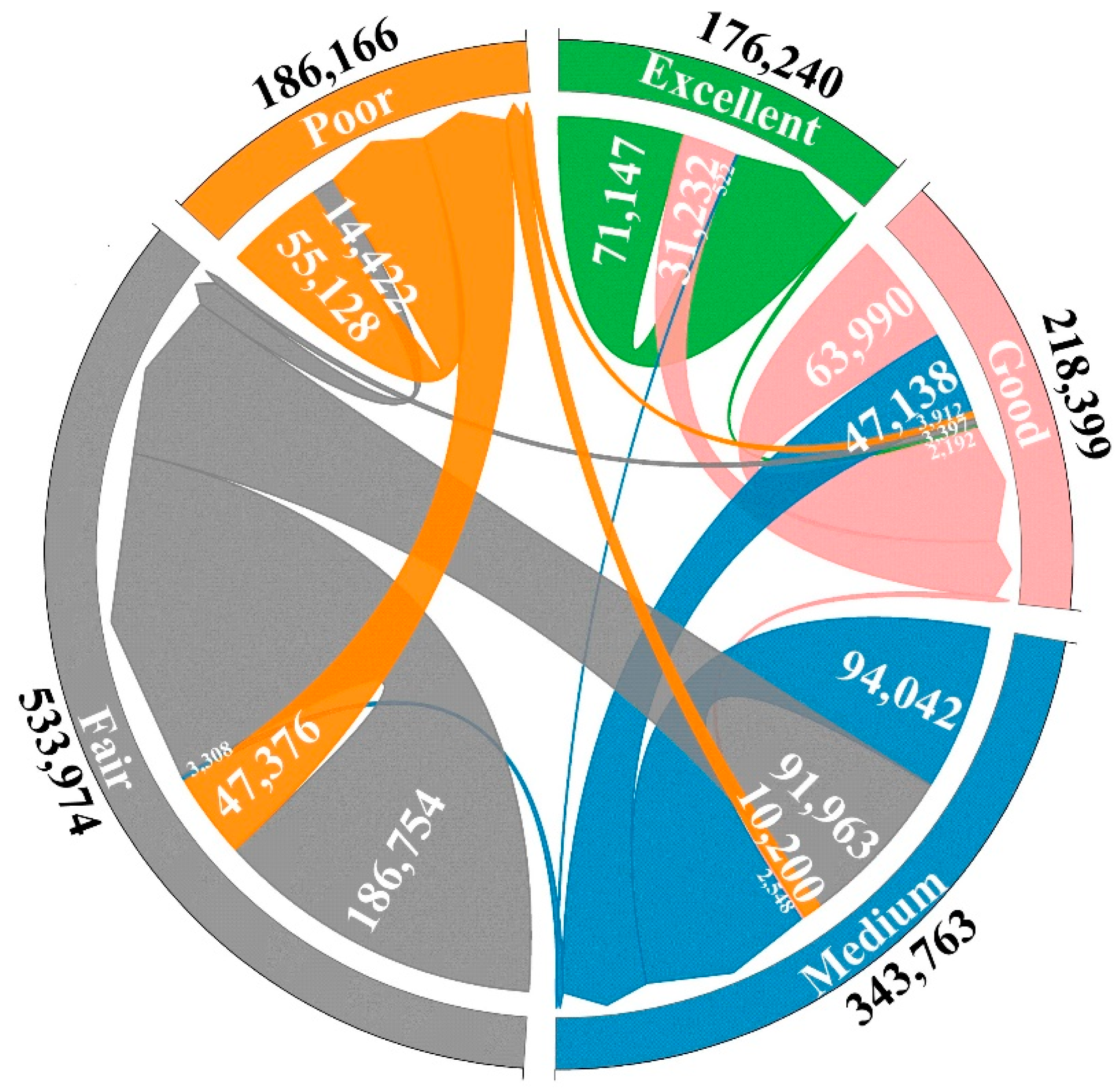
Figure 6a,b indicate an obvious circle structure in the spatial distribution of the VQI in both study years, with the values gradually increasing from the center to the periphery. Meanwhile, we can also see that the fair and poor levels of the VQI areas showed a larger expansion trend within the city from 2000 to 2016. Figure 6c reveals the temporal variation of the VQI between 2000 and 2016. Our calculations revealed that the unchanging area still represented the majority, accounting for 65.5% of the study area; a considerable proportion of the study area was degraded, accounting for 31.4%, while only a small proportion of the study area was improved, accounting for 3.1%. As shown in Figure 8, most of the transitions (93.0%) of the VQI classes occurred between adjacent levels, and only a small number of transitions (7.0%) occurred across multiple levels. The latter mainly occurred in the transformation from a good level of the VQI to fair and poor levels of the VQI, or from a medium level of the VQI to a poor level of the VQI.
4. Discussion
An ideal ecological index must have three basic properties: representativeness, measurability, and effectiveness [24,34,36]. Representativeness requires that the proposed index should objectively and comprehensively reflect the characteristics of an ecosystem. The representativeness of our proposed index was reflected in several aspects. Firstly, this index includes not only indicators of vegetation physical structure (i.e., AI, PLAND, and PD), but also an indicator of vegetation quality (i.e., NDVI). In terms of the indicators of the vegetation physical structure, they cover both the landscape composition and the spatial configuration metrics, measuring patch magnitude without spatial attributes, as well as patch locations in a spatial context. These three metrics are the most intuitive and frequently used class metrics [31,33]. Secondly, to overcome the shortcomings of most ecological indices composed only from a localized perspective and ignoring the spatial context [37], this proposed index holistically considers the quality of the pixel itself, as well as the effect of the surrounding environment. This is because each measurement has its own influence on the surrounding or external environment [10]. Lastly, one challenge in constructing a comprehensive index is assigning weights to each indicator. The current main weighting methods are the analytic hierarchy process (AHP) and Delphi method [38,39]. However, these methods are relatively subjective and are greatly influenced by human experience. In this study, we employed PCA, which is totally free from interference, to calculate the weights of each variable; thus, the VQI can be used to assess the urban vegetation status more objectively and easily. The percentage eigenvalues of PC1 were 94.014% and 92.192% for a window size of 3 km in 2000 and 2016, respectively. We further used correlation analysis and bivariate spatial autocorrelation analysis to explore the relationship between the VQI and the various indicators from the perspective of traditional statistics and spatial statistics (Table 4). Table 4 shows that the VQI and all indicators were all significantly correlated (p < 0.01). These results all confirm the representativeness of the VQI proposed in terms of all constitutive factors, especially PLAND, AI, and NDVI.
In addition, all the indicators can be quickly calculated using a moving window strategy. However, it should be noted that the scale of input data or analysis can impact the values of landscape metrics [33]. With the development of spatial analysis technology in recent decades, the scale effects (e.g., spatial extent, grain size, and cell resolution) of landscape metrics have become a global hotspot in landscape ecology studies. We also discussed the scale effects of the proposed VQI computed at different window sizes, and we identified the optimal analysis window size (i.e., 3 km) (Table 2 and Table 3, Figure 3 and Figure 4). Our research results confirm the existence of the scale effect of the landscape metrics [33], demonstrating that the analysis window size also impacts the values of landscape metrics.
In terms of the effectivity of the calculated VQI, a validity evaluation was implemented using correlation analysis. Table 4 shows that the VQI was significant correlated with various indicators. Moreover, the average correlation coefficients between the VQI and each variable were higher than those of any other factor pairs. These results highlight the superiority of the proposed VQI in terms of effectivity and representativeness. An interesting phenomenon is that NDVI revealed an obvious vegetation increase from 0.555 in 2000 to 0.654 in 2016, while the VQI has decreased slightly from 0.492 in 2000 to 0.424 in 2016 (Table 1). To prove which of these seemingly contradictory indicators was more effective, LST was employed as a response proxy, because vegetation has been widely considered to be responsible for urban heat island mitigation [9,40]. Pearson correlation and bivariate spatial autocorrelation observed that all the indicators were significantly related to LST except for NDVI in 2000. As expected, the VQI had the highest explanatory power for LST among all the factors in both of the studied years except for AI in 2000. However, unexpectedly, NDVI was found to be not highly correlated with LST in both of the studied years for the study area. This empirical case agrees with the results of multiple studies with regard to understanding the effect of greenspace on the urban heat environment [5,34], which revealed that the percentage of vegetation (PLAND) has a great impact the urban heat environment, while the R2 between NDVI and LST was not high according to the ordinary least square (OLS) model. On one hand, this confirms that the proposed index considering both the pixel itself and the surrounding environment has a greater impact on LST than indices only considering the pixel itself, and that the VQI can explain the urban thermal environment more effectively. On the other hand, it should be noted that the relationship between LST and its impactors may vary across locations [5]. Thus, Hu and Xu [34] employed a local regression model to explore the spatial non-stationarity in the relationships between the urban heat environment and land-cover features. The application of the local model greatly improved the regression coefficients (R2) of LST and NDVI. This also confirms the finding that the location of vegetation greatly affects the urban thermal environment [5]. Our result is in line with these previous studies, demonstrating a high negative correlation between AI and LST, which indicates that more concentrated vegetation in space contributes to a lower urban thermal environment.
Lastly, we used a histogram of the proposed VQI (Figure 6) and its spatiotemporal, observing that the quality of vegetation in the study area showed a downward trend during the study period. We also detected places (red areas in Figure 6) where the vegetation quality degraded between 2000 and 2016. This was mainly due to changes caused by the encroachment of vegetation land by construction land in the process of urbanization. These degraded areas are in good agreement with the areas of reduced vegetation in Figure 1. Since 2000, the island surrounded by the two rivers in the middle of the study area has ushered in large-scale urbanization [21]. This also reflects the objectivity of our proposed index (VQI), which could be successfully used to detect the status of and changes in vegetation quality in this study area at the pixel level.
This index can also be applied for the evaluation of spatiotemporal changes in vegetation quality in other regions, but attention should be paid to the selection of an appropriate moving window size when calculating the landscape class-level metrics. It should be noted that the principal components after dimensionality reduction through PCA are orthogonal, which can eliminate factors influencing the original data. PCA can retain most of the main information of the composed indices. The standard for PCA dimensionality reduction is to select the principal component that maximizes the variance of the original data on the new coordinate axis. However, features with small variance are not necessarily unimportant, and such a unique criterion may lose some important information of the vegetation. Moreover, PCA depends strongly on the ranges, distributions, and correlations of the observed datasets. When using the same variables but sampled at different sites, these relationships might differ substantially. Therefore, the quantities and interpretation of the VQI will change from site to site and from study to study.
5. Conclusions
In this study, a new index, the VQI, was constructed to detect urban vegetation quality. The VQI was synthesized using the PCA technique on the basis of four indicators: AI, PD, PLAND, and NDVI, thereby holistically considering both the quality of the vegetation and its spatial relationship with the surroundings. With the merit of objectivity in assigning weights for each variable using principal component analysis (PCA), the calculation of the index was totally free of artificial interference. The moving window strategy, Pearson correlation analysis, and bivariate spatial autocorrelation analysis were employed to validate the proposed index. The results showed that the percentage eigenvalues of PC1 were 94.014% and 92.192% for the 3 km window size in 2000 and 2016, respectively. The VQI had the greatest explanatory power for LST among all factors in both of the studied years except for AI in 2000, with its interpretation of LST being 0–44% better than any other indicator. We also conclude that the spatial location of vegetation has a great impact on the LST, with more concentrated vegetation in space contributing to a lower urban thermal environment.
Author Contributions
Conceptualization, X.H.; methodology, X.H.; software, X.H. and S.L.; formal analysis, X.H.; data curation, C.X. and J.C.; writing—original draft preparation, X.H.; writing—review and editing, R.Q.; visualization, Z.W. and R.Q.; supervision, Y.L. All authors have read and agreed to the published version of the manuscript.
Funding
This research was funded by the National Natural Science Foundation of China (No. 31971639 and No. 41901221), the Natural Science Foundation of Fujian Province (No. 2019J01406), and the Foundation for National Science and Technology Basic Resources Investigation Project (2019FY202108).
Institutional Review Board Statement
Not applicable.
Informed Consent Statement
Not applicable.
Data Availability Statement
The data are contained within the article, and all data sources are mentioned.
Conflicts of Interest
The authors declare no conflict of interest.
References
- Liu, X.; Huang, Y.; Xu, X.; Li, X.; Li, X.; Ciais, P.; Lin, P.; Gong, K.; Ziegler, A.D.; Chen, A. High-spatiotemporal-resolution mapping of global urban change from 1985 to 2015. Nat. Sustain. 2020, 3, 564–570. [Google Scholar] [CrossRef]
- Seto, K.C.; Güneralp, B.; Hutyra, L.R. Global forecasts of urban expansion to 2030 and direct impacts on biodiversity and carbon pools. Proc. Natl. Acad. Sci. USA 2012, 109, 16083–16088. [Google Scholar] [CrossRef] [PubMed] [Green Version]
- Peng, J.; Tian, L.; Liu, Y.; Zhao, M.; Wu, J. Ecosystem services response to urbanization in metropolitan areas: Thresholds identification. Sci. Total Environ. 2017, 607, 706–714. [Google Scholar] [CrossRef] [PubMed]
- Pickard, B.R.; Van Berkel, D.; Petrasova, A.; Meentemeyer, R.K. Forecasts of urbanization scenarios reveal trade-offs between landscape change and ecosystem services. Landsc. Ecol. 2017, 32, 617–634. [Google Scholar] [CrossRef]
- Guo, G.; Wu, Z.; Cao, Z.; Chen, Y.; Zheng, Z. Location of greenspace matters: A new approach to investigating the effect of the greenspace spatial pattern on urban heat environment. Landsc. Ecol. 2021, 36, 1533–1548. [Google Scholar] [CrossRef]
- Alonzo, M.; Bookhagen, B.; McFadden, J.P.; Sun, A.; Roberts, D.A. Mapping urban forest leaf area index with airborne lidar using penetration metrics and allometry. Remote Sens. Environ. 2015, 162, 141–153. [Google Scholar] [CrossRef]
- Escobedo, F.J.; Nowak, D.J. Spatial heterogeneity and air pollution removal by an urban forest. Landsc. Urban Plan. 2009, 90, 102–110. [Google Scholar] [CrossRef]
- McPherson, E.G.; Simpson, J.R.; Xiao, Q.; Wu, C. Million trees Los Angeles canopy cover and benefit assessment. Landsc. Urban Plan. 2011, 99, 40–50. [Google Scholar] [CrossRef]
- Greene, C.S.; Kedron, P.J. Beyond fractional coverage: A multilevel approach to analyzing the impact of urban tree canopy structure on surface urban heat islands. Appl. Geogr. 2018, 95, 45–53. [Google Scholar] [CrossRef]
- Afizzul, M.M.; Yasmin, Y.S.; Hamdan, O. Development of landscape forest performance index to assess forest quality of managed forests. In Proceedings of the IOP Conference Series: Earth and Environmental Science, Kuala Lumpur, Malaysia, 20–21 October 2020; Volumer 540, p. 12012. [Google Scholar] [CrossRef]
- Becker, S.J.; Daughtry, C.S.T.; Russ, A.L. Robust forest cover indices for multispectral images. Photogramm. Eng. Remote Sens. 2018, 84, 505–512. [Google Scholar] [CrossRef]
- Lim, K.; Treitz, P.; Baldwin, K.; Morrison, I.; Green, J. Lidar remote sensing of biophysical properties of tolerant northern hardwood forests. Can. J. Remote Sens. 2003, 29, 658–678. [Google Scholar] [CrossRef]
- Pettorelli, N.; Vik, J.O.; Mysterud, A.; Gaillard, J.-M.; Tucker, C.J.; Stenseth, N.C. Using the satellite-derived NDVI to assess ecological responses to environmental change. Trends Ecol. Evol. 2005, 20, 503–510. [Google Scholar] [CrossRef] [PubMed]
- Myneni, R.B.; Hall, F.G.; Sellers, P.J.; Marshak, A.L. The interpretation of spectral vegetation indexes. IEEE Trans. Geosci. Remote Sens. 1995, 33, 481–486. [Google Scholar] [CrossRef]
- Carlson, T.N.; Ripley, D.A. On the relation between NDVI, fractional vegetation cover, and leaf area index. Remote Sens. Environ. 1997, 62, 241–252. [Google Scholar] [CrossRef]
- Hardin, P.J.; Jensen, R.R. The effect of urban leaf area on summertime urban surface kinetic temperatures: A Terre Haute case study. Urban For. urban Green. 2007, 6, 63–72. [Google Scholar] [CrossRef]
- Cattanio, J.H. Leaf area index and root biomass variation at different secondary forest ages in the eastern Amazon. For. Ecol. Manag. 2017, 400, 1–11. [Google Scholar] [CrossRef]
- Chen, L.; Wang, Y.; Ren, C.; Zhang, B.; Wang, Z. Optimal combination of predictors and algorithms for forest above-ground biomass mapping from sentinel and SRTM data. Remote Sens. 2019, 11, 414. [Google Scholar] [CrossRef] [Green Version]
- Majasalmi, T.; Rautiainen, M. The potential of Sentinel-2 data for estimating biophysical variables in a boreal forest: A simulation study. Remote Sens. Lett. 2016, 7, 427–436. [Google Scholar] [CrossRef]
- Wiggins, H.L.; Nelson, C.R.; Larson, A.J.; Safford, H.D. Using LiDAR to develop high-resolution reference models of forest structure and spatial pattern. For. Ecol. Manag. 2019, 434, 318–330. [Google Scholar] [CrossRef]
- Hu, X.; Xu, H. A new remote sensing index for assessing the spatial heterogeneity in urban ecological quality: A case from Fuzhou City, China. Ecol. Indic. 2018, 89, 11–21. [Google Scholar] [CrossRef]
- Xu, H.; Wang, Y.; Guan, H.; Shi, T.; Hu, X. Detecting ecological changes with a remote sensing based ecological index (RSEI) produced time series and change vector analysis. Remote Sens. 2019, 11, 2345. [Google Scholar] [CrossRef] [Green Version]
- Liu, S.; Li, X.; Chen, L.; Zhao, Q.; Zhao, C.; Hu, X.; Li, J. A New Approach to Investigate the Spatially Heterogeneous in the Cooling Effects of Landscape Pattern. Land 2022, 11, 239. [Google Scholar] [CrossRef]
- Hu, X.; Xu, H. A new remote sensing index based on the pressure-state-response framework to assess regional ecological change. Environ. Sci. Pollut. Res. 2019, 26, 5381–5393. [Google Scholar] [CrossRef] [PubMed]
- Jiménez-Muñoz, J.C.; Sobrino, J.A.; Skoković, D.; Mattar, C.; Cristóbal, J. Land surface temperature retrieval methods from Landsat-8 thermal infrared sensor data. IEEE Geosci. Remote Sens. Lett. 2014, 11, 1840–1843. [Google Scholar] [CrossRef]
- Bodin, Ö.; Saura, S. Ranking individual habitat patches as connectivity providers: Integrating network analysis and patch removal experiments. Ecol. Modell. 2010, 221, 2393–2405. [Google Scholar] [CrossRef]
- Fernandes, M.R.; Aguiar, F.C.; Ferreira, M.T. Assessing riparian vegetation structure and the influence of land use using landscape metrics and geostatistical tools. Landsc. Urban Plan. 2011, 99, 166–177. [Google Scholar] [CrossRef] [Green Version]
- Sowińska-Świerkosz, B.N.; Soszyński, D. Landscape structure versus the effectiveness of nature conservation: Roztocze region case study (Poland). Ecol. Indic. 2014, 43, 143–153. [Google Scholar] [CrossRef]
- Zhou, W.; Huang, G.; Cadenasso, M.L. Does spatial configuration matter? Understanding the effects of land cover pattern on land surface temperature in urban landscapes. Landsc. Urban Plan. 2011, 102, 54–63. [Google Scholar] [CrossRef]
- McGarigal, K.; Marks, B. FRAGSTATS: Spatial Pattern Analysis Program for Quantifying Landscape Structure; U.S. Department of Agriculture, Forest Service, Pacific Northwest Research Station: Corvallis, OR, USA, 1995.
- Liu, J.; Wilson, M.; Hu, G.; Liu, J.; Wu, J.; Yu, M. How does habitat fragmentation affect the biodiversity and ecosystem functioning relationship? Landsc. Ecol. 2018, 33, 341–352. [Google Scholar] [CrossRef]
- Zhou, W.; Pickett, S.T.A.; Cadenasso, M.L. Shifting concepts of urban spatial heterogeneity and their implications for sustainability. Landsc. Ecol. 2017, 32, 15–30. [Google Scholar] [CrossRef]
- Šímová, P.; Gdulová, K. Landscape indices behavior: A review of scale effects. Appl. Geogr. 2012, 34, 385–394. [Google Scholar] [CrossRef]
- Hu, X.; Xu, H. Spatial variability of urban climate in response to quantitative trait of land cover based on GWR model. Environ. Monit. Assess. 2019, 191, 194. [Google Scholar] [CrossRef] [PubMed]
- Seddon, A.W.R.; Macias-Fauria, M.; Long, P.R.; Benz, D.; Willis, K.J. Sensitivity of global terrestrial ecosystems to climate variability. Nature 2016, 531, 229–232. [Google Scholar] [CrossRef] [PubMed] [Green Version]
- Lin, T.; Ge, R.; Huang, J.; Zhao, Q.; Lin, J.; Huang, N.; Zhang, G.; Li, X.; Ye, H.; Yin, K. A quantitative method to assess the ecological indicator system’s effectiveness: A case study of the ecological province construction indicators of China. Ecol. Indic. 2016, 62, 95–100. [Google Scholar] [CrossRef]
- Liu, Y.; Peng, J.; Wang, Y. Application of partial least squares regression in detecting the important landscape indicators determining urban land surface temperature variation. Landsc. Ecol. 2018, 33, 1133–1145. [Google Scholar] [CrossRef]
- Cinelli, M.; Coles, S.R.; Kirwan, K. Analysis of the potentials of multi criteria decision analysis methods to conduct sustainability assessment. Ecol. Indic. 2014, 46, 138–148. [Google Scholar] [CrossRef] [Green Version]
- Norouzian-Maleki, S.; Bell, S.; Hosseini, S.-B.; Faizi, M. Developing and testing a framework for the assessment of neighbourhood liveability in two contrasting countries: Iran and Estonia. Ecol. Indic. 2015, 48, 263–271. [Google Scholar] [CrossRef] [Green Version]
- Taylor, L.; Hochuli, D.F. Defining greenspace: Multiple uses across multiple disciplines. Landsc. Urban Plan. 2017, 158, 25–38. [Google Scholar] [CrossRef] [Green Version]
Figure 1.
Location of Fuzhou City and spatial distribution of greenspace: (a) study area; (b,c) spatial distribution of greenspace in 2000 and 2016, respectively.
Figure 1.
Location of Fuzhou City and spatial distribution of greenspace: (a) study area; (b,c) spatial distribution of greenspace in 2000 and 2016, respectively.

Figure 2.
Spatial distribution of landscape metrics using a window size of 3 km: (a,b) calculated NDVI for each cell (30 m spatial resolution) within a 3 km neighborhood using the focal statistics tool in ArcGIS software in 2000 and 2016; (c,d) calculated AI in 2000 and 2016; (e,f) calculated PD in 2000 and 2016; (g,h) calculated PLAND in 2000 and 2016.

Figure 3.
Box plot of correlation coefficients between VQI indicators for different moving window sizes. The red box indicates the year 2000, while the blue box indicates the year 2016.
Figure 3.
Box plot of correlation coefficients between VQI indicators for different moving window sizes. The red box indicates the year 2000, while the blue box indicates the year 2016.

Figure 4.
Changes in percentage eigenvalue of PC1 for different moving widow sizes.

Figure 5.
Histogram and kernel smooth curves of the vegetation ecological quality in 2000 and 2016.

Figure 6.
Spatial distribution in the VQI and its changes in 2000 and 2016: (a) 2000; (b) 2016; (c) change in VQI between 2000 and 2016.
Figure 6.
Spatial distribution in the VQI and its changes in 2000 and 2016: (a) 2000; (b) 2016; (c) change in VQI between 2000 and 2016.

Figure 7.
The area ratio of each VQI class in 2000 and 2016.

Figure 8.
Chord diagram of the transfer matrix between different levels of VQI during 2000 and 2016. Different colors represent different levels of the VQI, while the number on the outer ring represents the initial area of each level in 2000 plus the area transferred in during the study period of 2000 and 2016, including self-transferred areas. The direction of the arrow indicates the direction of transfer among different levels, while the number on the arrow indicates the amount of area transferred. The outer and inner values indicate the number of cells at the beginning of the period and the number of cells transferred during 2000 and 2016.


Table 1.
Statistics of each indicator of VQI (3 km window size).
| 2000 | 2016 | |||||||||||
|---|---|---|---|---|---|---|---|---|---|---|---|---|
| AI | PD | PLAND | NDVI | VQI 1 | VQI 2 | AI | PD | PLAND | NDVI | VQI 1 | VQI 2 | |
| Maximum | 99.801 | 24.507 | 99.637 | 0.835 | 128.343 | 1 | 99.886 | 23.527 | 99.853 | 0.915 | 133.269 | 1 |
| Minimum | 13.636 | 0.109 | 0.118 | 0.286 | 4.897 | 0 | 18.280 | 0.109 | 0.520 | 0.435 | 8.217 | 0 |
| Mean | 82.163 | 6.484 | 39.534 | 0.555 | 65.625 | 0.492 | 77.743 | 7.593 | 30.827 | 0.654 | 61.194 | 0.424 |
| SD | 11.887 | 4.096 | 27.130 | 0.102 | 28.992 | 0.235 | 14.812 | 4.169 | 26.611 | 0.104 | 29.515 | 0.236 |
Note: VQI 1 and VQI 2 refer to the original value and the normalized value, respectively.
Table 2.
Correlation matrix of VQI indicators.
| Window Size | 2000 | 2016 | |||||||
|---|---|---|---|---|---|---|---|---|---|
| Index | PD | PLAND | AI | NDVI | PD | PLAND | AI | NDVI | |
| 500 m | PD | 1.000 | 1.000 | ||||||
| PLAND | −0.462 ** | 1.000 | −0.380 ** | 1.000 | |||||
| AI | −0.594 ** | 0.733 ** | 1.000 | −0.458 ** | 0.706 ** | 1.000 | |||
| NDVI | −0.098 ** | 0.548 ** | 0.321 ** | 1.000 | −0.073 ** | 0.533 ** | 0.314 ** | 1.000 | |
| 1 km | PD | 1.000 | 1.000 | ||||||
| PLAND | −0.417 ** | 1.000 | −0.433 ** | 1.000 | |||||
| AI | −0.482 ** | 0.761 ** | 1.000 | ** | −0.390 ** | 0.768 ** | 1.000 | ||
| NDVI | −0.029 * | 0.653 ** | 0.402 ** | 1.000 | −0.040 ** | 0.603 ** | 0.406 ** | 1.000 | |
| 2 km | PD | 1.000 | 1.000 | ||||||
| PLAND | −0.424 ** | 1.000 | −0.519 ** | 1.000 | |||||
| AI | −0.400 ** | 0.808 ** | 1.000 | −0.502 ** | 0.812 ** | 1.000 | |||
| NDVI | −0.053 ** | 0.666 ** | 0.457 ** | 1.000 | −0.116 ** | 0.590 ** | 0.421 ** | 1.000 | |
| 3 km | PD | 1.000 | 1.000 | ||||||
| PLAND | −0.454 ** | 1.000 | −0.563 ** | 1.000 | |||||
| AI | −0.428 ** | 0.822 ** | 1.000 | * | −0.583 ** | 0.808 ** | 1.000 | ||
| NDVI | −0.229 ** | 0.603 ** | 0.603 ** | 1.000 | −0.312 ** | 0.841 ** | 0.600 ** | 1.000 | |
| 4 km | PD | 1.000 | 1.000 | ||||||
| PLAND | −0.487 ** | 1.000 | −0.600 ** | 1.000 | |||||
| AI | −0.463 ** | 0.815 ** | 1.000 | −0.633 ** | 0.800 ** | 1.000 | |||
| NDVI | −0.163 ** | 0.602 ** | 0.403 ** | 1.000 | −0.207 ** | 0.543 ** | 0.388 ** | 1.000 | |
| 5 km | PD | 1.000 | 1.000 | ||||||
| PLAND | −0.522 ** | 1.000 | −0.642 ** | 1.000 | |||||
| AI | −0.509 ** | 0.812 ** | 1.000 | * | −0.681 ** | 0.801 ** | 1.000 | ||
| NDVI | −0.210 ** | 0.572 ** | 0.394 ** | 1.000 | −0.238 ** | 0.524 ** | 0.381 ** | 1.000 | |
Note: ** indicates significance at 0.01 level, * indicates significance at 0.05 level.
Table 3.
Principal component analysis of VQI (eigenvalues and eigenvectors).
| Window Size | 2000 | 2016 | |||||||
|---|---|---|---|---|---|---|---|---|---|
| Index | PC1 | PC2 | PC3 | PC4 | PC1 | PC2 | PC3 | PC4 | |
| 500 m | PD | −0.142 | −0.409 | 0.901 | −0.004 | −0.108 | −0.156 | 0.982 | −0.004 |
| PLAND | 0.905 | −0.423 | −0.050 | −0.005 | 0.850 | −0.527 | 0.009 | −0.005 | |
| AI | 0.402 | 0.808 | 0.430 | 0.001 | 0.516 | 0.835 | 0.189 | 0.001 | |
| NDVI | 0.003 | −0.004 | 0.003 | 1.000 | 0.003 | −0.004 | 0.003 | 1.000 | |
| Eigenvalue | 685.947 | 72.226 | 27.050 | 0.017 | 767.722 | 111.525 | 33.236 | 0.020 | |
| Percentage eigenvalue (%) | 87.355 | 9.198 | 3.445 | 0.002 | 84.134 | 12.222 | 3.642 | 0.002 | |
| 1 km | PD | −0.092 | −0.217 | 0.972 | −0.008 | −0.083 | −0.003 | 0.997 | −0.009 |
| PLAND | 0.914 | −0.406 | −0.004 | −0.006 | 0.854 | −0.516 | 0.069 | −0.006 | |
| AI | 0.395 | 0.888 | 0.235 | 0.002 | 0.514 | 0.857 | 0.045 | 0.001 | |
| NDVI | 0.004 | −0.005 | 0.008 | 1.000 | 0.004 | −0.004 | 0.010 | 1.000 | |
| Eigenvalue | 673.721 | 55.926 | 19.810 | 0.013 | 725.153 | 77.561 | 19.220 | 0.017 | |
| Percentage eigenvalue (%) | 89.893 | 7.462 | 2.643 | 0.002 | 88.223 | 9.436 | 2.338 | 0.002 | |
| 2 km | PD | −0.070 | −0.054 | 0.996 | −0.011 | −0.083 | −0.044 | 0.996 | −0.012 |
| PLAND | 0.920 | −0.390 | 0.044 | −0.007 | 0.882 | −0.469 | 0.053 | −0.007 | |
| AI | 0.386 | 0.919 | 0.077 | 0.003 | 0.464 | 0.882 | 0.077 | 0.002 | |
| NDVI | 0.004 | −0.006 | 0.011 | 1.000 | 0.004 | −0.005 | 0.012 | 1.000 | |
| Eigenvalue | 566.461 | 33.652 | 11.538 | 0.012 | 572.231 | 42.645 | 9.373 | 0.018 | |
| Percentage eigenvalue (%) | 92.610 | 5.502 | 1.886 | 0.002 | 91.665 | 6.831 | 1.501 | 0.003 | |
| 3 km | PD | −0.066 | −0.055 | 0.996 | −0.005 | −0.084 | −0.090 | 0.992 | −0.005 |
| PLAND | 0.932 | −0.359 | 0.042 | −0.004 | 0.894 | −0.448 | 0.035 | −0.004 | |
| AI | 0.355 | 0.932 | 0.075 | 0.002 | 0.441 | 0.890 | 0.118 | 0.001 | |
| NDVI | 0.003 | −0.004 | 0.005 | 1.000 | 0.003 | −0.003 | 0.005 | 1.000 | |
| Eigenvalue | 454.260 | 21.849 | 7.076 | 0.001 | 480.369 | 34.674 | 6.100 | 0.001 | |
| Percentage eigenvalue (%) | 94.014 | 4.522 | 1.464 | 0.000 | 92.192 | 6.655 | 1.153 | 0.000 | |
| 4 km | PD | −0.065 | −0.065 | 0.996 | −0.009 | −0.085 | −0.102 | 0.991 | −0.011 |
| PLAND | 0.941 | −0.337 | 0.040 | −0.007 | 0.901 | −0.434 | 0.033 | −0.006 | |
| AI | 0.333 | 0.939 | 0.083 | 0.005 | 0.426 | 0.895 | 0.129 | 0.001 | |
| NDVI | 0.005 | −0.008 | 0.009 | 1.000 | 0.004 | −0.005 | 0.011 | 1.000 | |
| Eigenvalue | 389.680 | 17.760 | 4.925 | 0.015 | 420.534 | 30.458 | 4.277 | 0.020 | |
| Percentage eigenvalue (%) | 94.496 | 4.307 | 1.194 | 0.004 | 92.366 | 6.690 | 0.940 | 0.004 | |
| 5 km | PD | −0.066 | −0.086 | 0.994 | −0.007 | −0.087 | −0.112 | 0.990 | −0.011 |
| PLAND | 0.947 | −0.318 | 0.035 | −0.007 | 0.907 | −0.419 | 0.032 | −0.006 | |
| AI | 0.313 | 0.944 | 0.103 | 0.004 | 0.411 | 0.901 | 0.138 | 0.001 | |
| NDVI | 0.005 | −0.007 | 0.007 | 1.000 | 0.005 | −0.004 | 0.011 | 1.000 | |
| Eigenvalue | 332.156 | 14.022 | 3.468 | 0.017 | 370.479 | 25.468 | 3.078 | 0.021 | |
| Percentage eigenvalue (%) | 94.993 | 4.010 | 0.992 | 0.005 | 92.841 | 6.382 | 0.771 | 0.005 | |
Note: PC1–PC4 refer to the first to fourth principal components, respectively.
Table 4.
Correlations between the VQI and all indicators (3 km).
| Indicators | Index | AI | PD | PLAND | NDVI | Average 1 |
|---|---|---|---|---|---|---|
| 2000 | R2 | 0.866 ** | −0.469 ** | 0.996 ** | 0.840 ** | 0.793 |
| Moran’s I | 0.828 ** | −0.440 ** | 0.956 ** | 0.822 ** | 0.762 | |
| 2016 | R2 | 0.879 ** | −0.589 ** | 0.991 ** | 0.820 ** | 0.820 |
| Moran’s I | 0.841 ** | −0.561 ** | 0.952 ** | 0.803 ** | 0.789 |
Note: ** statistically significant at the 0.01 level, l 1 the value of the correlation was the average of the absolute value of each correlation coefficient.
Table 5.
Correlations between VQI and LST.
| Year | Indicator | AI | PD | PLAND | NDVI | VQI |
|---|---|---|---|---|---|---|
| 2000 | Pearson correlation | −0.515 ** | 0.179 ** | −0.350 ** | −0.011 | −0.382 ** |
| Moran’s I | −0.508 ** | 0.170 ** | −0.343 ** | −0.047 * | −0.375 ** | |
| 2016 | Pearson correlation | −0.505 ** | 0.454 ** | −0.494 ** | −0.078 ** | −0.515 ** |
| Moran’s I | −0.495 ** | 0.437 ** | −0.479 ** | −0.121 ** | −0.501 ** |
Note: ** statistically significant at the 0.01 level, * statistically significant at the 0.05 level.
Publisher’s Note: MDPI stays neutral with regard to jurisdictional claims in published maps and institutional affiliations. |
© 2022 by the authors. Licensee MDPI, Basel, Switzerland. This article is an open access article distributed under the terms and conditions of the Creative Commons Attribution (CC BY) license (https://creativecommons.org/licenses/by/4.0/).
Share and Cite
MDPI and ACS Style
Hu, X.; Xu, C.; Chen, J.; Lin, Y.; Lin, S.; Wu, Z.; Qiu, R. A Synthetic Landscape Metric to Evaluate Urban Vegetation Quality: A Case of Fuzhou City in China. Forests 2022, 13, 1002. https://doi.org/10.3390/f13071002
AMA Style
Hu X, Xu C, Chen J, Lin Y, Lin S, Wu Z, Qiu R. A Synthetic Landscape Metric to Evaluate Urban Vegetation Quality: A Case of Fuzhou City in China. Forests. 2022; 13(7):1002. https://doi.org/10.3390/f13071002
Chicago/Turabian StyleHu, Xisheng, Chongmin Xu, Jin Chen, Yuying Lin, Sen Lin, Zhilong Wu, and Rongzu Qiu. 2022. "A Synthetic Landscape Metric to Evaluate Urban Vegetation Quality: A Case of Fuzhou City in China" Forests 13, no. 7: 1002. https://doi.org/10.3390/f13071002
Note that from the first issue of 2016, this journal uses article numbers instead of page numbers. See further details here.