Finer Resolution Estimation and Mapping of Mangrove Biomass Using UAV LiDAR and WorldView-2 Data
by
 , ,
, ,
Penghua Qiu
1, 
Dezhi Wang
2,*,
Xinqing Zou
3,
Xing Yang
1,
Genzong Xie
1,
Songjun Xu
4 and
Zunqian Zhong
1 1
College of Geography and Environmental Science, Hainan Normal University, Haikou 571158, China
2
Faculty of Information Engineering, China University of Geosciences (Wuhan), Wuhan 430074, China
3
School of Geography and Ocean Science, Nanjing University, Nanjing 210023, China
4
School of Geography, South China Normal University, Guangzhou 510631, China
*
Author to whom correspondence should be addressed.
Forests 2019, 10(10), 871; https://doi.org/10.3390/f10100871
Submission received: 31 July 2019
/
Revised: 24 September 2019
/
Accepted: 26 September 2019
/
Published: 4 October 2019
(This article belongs to the Special Issue Applications of Remote Sensing Data in Mapping of Forest Growing Stock and Biomass)
Abstract
:To estimate mangrove biomass at finer resolution, such as at an individual tree or clump level, there is a crucial need for elaborate management of mangrove forest in a local area. However, there are few studies estimating mangrove biomass at finer resolution partly due to the limitation of remote sensing data. Using WorldView-2 imagery, unmanned aerial vehicle (UAV) light detection and ranging (LiDAR) data, and field survey datasets, we proposed a novel method for the estimation of mangrove aboveground biomass (AGB) at individual tree level, i.e., individual tree-based inference method. The performance of the individual tree-based inference method was compared with the grid-based random forest model method, which directly links the field samples with the UAV LiDAR metrics. We discussed the feasibility of the individual tree-based inference method and the influence of diameter at breast height (DBH) on individual segmentation accuracy. The results indicated that (1) The overall classification accuracy of six mangrove species at individual tree level was 86.08%. (2) The position and number matching accuracies of individual tree segmentation were 87.43% and 51.11%, respectively. The number matching accuracy of individual tree segmentation was relatively satisfying within 8 cm ≤ DBH ≤ 30 cm. (3) The individual tree-based inference method produced lower accuracy than the grid-based RF model method with R2 of 0.49 vs. 0.67 and RMSE of 48.42 Mg ha−1 vs. 38.95 Mg ha−1. However, the individual tree-based inference method can show more detail of spatial distribution of mangrove AGB. The resultant AGB maps of this method are more beneficial to the fine and differentiated management of mangrove forests.
1. Introduction
Mangroves have attracted considerable attention due to their unique morphological characteristics and diverse eco-environmental service functions [1]. These services include coastal protection, biodiversity maintenance, and carbon sequestration [2,3,4,5]. The organic carbon in mangrove forests per unit area is four times higher than that of other terrestrial forest ecosystems [6]. Mangroves are therefore considered a strong candidate for the United Nations Framework Convention on Climate Change (UNFCCC), the payments for ecosystem services (PES) program [7], and the policymaking and implementation in blue carbon. However, all these initiatives require accurate biomass and carbon stock estimations. The aboveground biomass (AGB) of mangroves is one of the fundamental parameters describing a mangrove ecosystem’s functioning and is essential for determining its storage of carbon. Accurate estimate of AGB is critical for mangrove monitoring and management. To build a beautiful China and protect the ecological marine environment, local governments of coastal areas in China have been asked to fully implement the bay chief system (A leader responsible system in governance of bays began in 2017, which was proposed by the State Oceanic Administration, China.) and conduct pilot work on carbon sinks in marine ecosystems. Strengthening the research on mangrove biomass will help to support this work.
Biomass estimation methods can be categorized into direct and indirect methods. The direct approach is a traditional field harvesting method. Among the indirect methods, the allometric estimation is the most common approach and has become a standard tool for biomass prediction [8]. The basic theory of allometric relationships suggests that in many organisms, the growth rate of one part of an organism is proportional to the growth rate of growth of another [9]. Thus, researchers have often used allometric regression equations based on available and measurable woody plant parameters such as stem diameter, tree height, or crown diameter to estimate biomass [10,11].
To improve the accuracy of mangrove biomass estimation and mapping, more remote sensing data and methods have been tested and applied to mangroves [4,12,13,14,15,16,17,18,19,20]. Very high resolution images, such as WorldView-2 (Digitalglobe, Westminster, CO, USA), GeoEye (GeoEye, Herndon, VA, USA), IKONOS (Spacing Imaging, Herndon, VA, USA), QuickBird (Digitalglobe, Westminster, CO, USA), digital photographs, and light detection and ranging (LiDAR) point cloud data, can be used for extracting individual trees [21,22,23,24,25,26], as well as the accurate estimation of AGB or carbon stocks at the individual tree level [27,28,29,30,31,32,33,34]. Yin and Wang (2019) used UAV LiDAR to study the individual tree detection and delineation (ITDD) of mangroves and proposed a rule-of-thumb that the spatial resolution should be finer than one-fourth of the crown diameter for ITDD [26]. To date, to the best of our knowledge, no study has discriminated mangrove species and estimated mangrove biomass in a finer resolution, such as individual tree or clump level. In addition, despite the wide use of remote sensing techniques to obtain and retrieve mangrove information, there is no general consensus approach [35]. Because of the ability to provide spectral information, optical images are considered to be very useful in distinguishing plant species [36]. While, LiDAR data can provide more information about forest structure [32,33]. Therefore, the integration use of very high spatial resolution WorldView-2 imagery and UAV LiDAR data may provide the potential for mangrove biomass estimation and mapping at finer resolution.
The overall aim of this study was to use optical remote sensing, UAV LiDAR, field survey data sets, and allometric equations to estimate and map the AGB of mangroves in Qinglan harbor, Hainan province, China. In this study, we aimed to (1) compare the merits and demerits of AGB estimation based on the newly proposed individual tree-based inference method and the grid-based RF model method, (2) examine the accuracies of AGB estimation for two methods, and (3) map the AGB of mangroves.
2. Materials and Methods
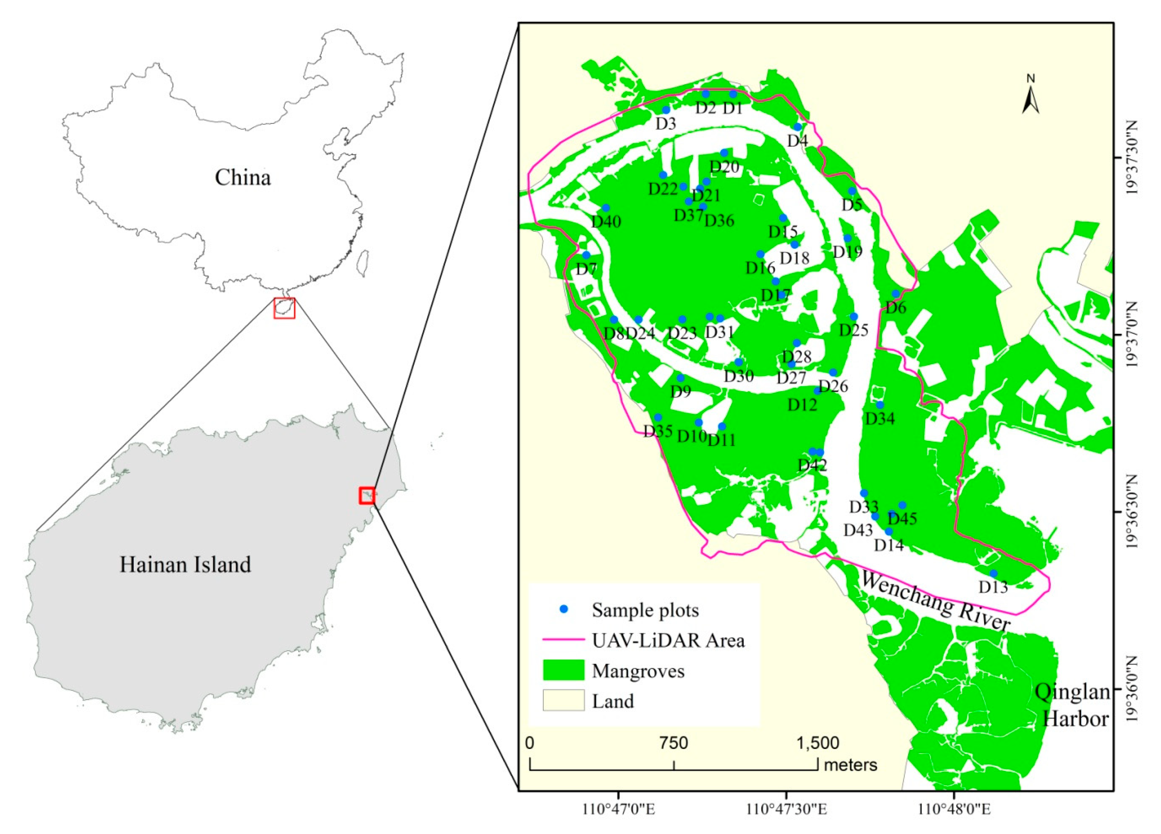
2.1. Study Site
The study was conducted in the core area of the Qinglan Harbor Provincial Nature Reserve, located on the northeastern part of Hainan Island, China (Figure 1). The Qinglan Harbor Nature Reserve is the reserve that has the most abundant mangrove species in China, including 24 true mangrove species and 10 semi-mangrove species, which account for 88.89% and 100% of the total number of true- and semi-mangrove species in China, respectively. In China, mangroves in the Qinglan Harbor Nature Reserve are distributed with the tallest plants, the oldest forests, the most complete community preservation, and many rare and endangered mangrove species. The total mangrove area of the Qinglan Harbor Nature Reserve is about 835.5 ha.
The study area was 386.32 ha, with a mangrove area of 209.99 ha. The landforms are mainly sea alluvial plain, lagoon plain, sea platform, and mangrove beach. The soil type is mostly alluvial soil with a smooth soil texture (silty clay). The mean annual temperature is about 24.1 ℃, the average annual rainfall is around 1650 mm and the average tidal range is about 0.89 m. The salinity of its water ranges between 3‰ and 25‰.
2.2. Field Data Collection
The field surveys were conducted from July to September 2018 and March 2019. A total of 45 plots were surveyed. The base plot area was 10 × 10 m, which was expanded up to 600 m2 depending on the specific field situation. All individual trees with a diameter at breast height (DBH) of ≥1.5cm and height that was ≥1.5 m within the plots were counted and measured for species, number, height, stem girth at breast height (GBH, cm; DBH = GBH/π), and crown cover. A real-time kinetic global positioning system (RTK-GPS) was used to measure the geographical position of each plot and most of measured trees. A total of 3832 individual trees and 13 species (Bruguiera sexangula (Lour.) Poir., Excoecaria agallocha Linn., Rhizophora apiculata Blume, Aegiceras corniculatum (Linn.) Blanco, Kandelia candel (Linn.) Druce, Xylocarpus granatum Koenig, Ceriops tagal (Perr.) C. B. Rob., Lumnitzera racemosa Willd., Heritiera littoralis Dryand., Hibiscus tiliaceus Linn., Sonneratia apetala Buch-Ham., Sonneratia alba J. Smith, Sonneratia ovata Backer) were recorded in the 45 field plots. 68.89% of the plots had at least 3 types of mangrove species. The mangrove forest was dominated by B. sexangula. The tree density of B. sexangula was highest among all mangrove species, which was 1.5 times and 2.0 times higher than that of E. agallocha and L. racemosa, respectively. The summary of the community structure of the mangrove forest in Qinglan Harbor Nature Reserve was presented in Table 1.
The AGB in each field plot was estimated by the allometric equation method. The selection principles were as follows: (1) Domestic models take precedence over foreign models; (2) the closer the study area of the model to Hainan, the more preferred it is; (3) the closest forest age takes precedence; and (4) species with similar DBH are preferred. When no specific allometric equation was available, a common allometric equation was used (Table 2). We first calculated the AGB of each tree using the species-specific allometric equations presented in Table 2 and then summed the AGBs in each field plot. To obtain the AGB density for each plot, we divided the summed AGB of a plot by the plot’s area.
2.3. Remote Sensing Data and Processing
2.3.1. WorldView-2 Imagery
The WorldView-2 optical images were acquired on 5 October 2018. They included a 0.5 m panchromatic band and eight 2.0 m multispectral bands.
First the images were radiometrically corrected. Then, the multispectral images were pan-sharpened by the panchromatic image using the NNDiffuse tool in ENVI 5.3 (Harris Geospatial, Melbourne, FL, USA). Finally, this pan-sharpened imagery was co-registered to the UAV LiDAR data. The precision was controlled within 0.5 pixels. The mangrove extent of the study area was extracted using this processed imagery. The detail process of how to extract mangrove extent using high spatial resolution imagery can refer to our previous work [45]. The main flowchart of remote sensing data processing and AGB estimation was presented in Figure 2.
2.3.2. UAV LiDAR Data and Mangrove Canopy Height Model Production
The UAV LiDAR data were collected in March 2018 using a Velodyne VLP-16 puck sensor (Velodyne LiDAR, San Jose, CA, USA) with a laser wavelength of 903 nm. The sensor can emit 300,000 points per second with an accuracy of 3 cm. The average point density was 94 points/m2. The flight elevation was 52 m with a speed of 5 m/s. An RTK-GPS was simultaneously used to obtain the base station position of the UAV LiDAR system with centimeter-level accuracy.
The raw LiDAR data were first computed using aerial triangulation algorithm to obtain accurate position of each LiDAR point cloud. Then, the noise and outlier points of the LiDAR data were filtered using LiDAR360 software (GreenValley, Beijing, China). Subsequently, the point clouds were classified as non-ground and ground points. The ground points were used to produce the digital elevation model (DEM) using the triangulated irregular net (TIN) interpolation method. Both the ground points and non-ground points were utilized to generate the digital surface model (DSM) using the inverse distance weighted (IDW) interpolation method. The canopy height model (CHM) was produced through subtracting the DEM from the DSM [5]. Finally, the point clouds were normalized using the DEM subtraction method [26] and masked by the mangrove extent, which was produced from the WorldView-2 imagery.
2.4. Mangrove Species Classification and Individual Tree Detection
The mangrove classification was conducted in the R language platform using random forest (RF) algorithm. RF, proposed by Leo Breiman (2001) [46], is an integrated machine learning algorithm based on decision trees. The bootstrap re-sampling is used to construct the decision tree model by randomly sampling from the original sample set. The final result is obtained by voting on the prediction of multiple decision trees. The RF algorithm can be used to classify remote sensing images with complex spatial distribution or to identify multiple data of different statistical distributions and scales.
From the spectral curves of different mangrove species in Figure 3 and the 0.5 m pan-sharpened WorldView-2 imagery, we found that S. ovata, S. apetala, and S. alba communities and the mixed community of S. ovata and A. corniculatum have similar appearances, textures, and spectral features overall, which means they are difficult to separate. In addition, S. ovata, S. apetala, and S. alba belong to the same genus of Sonneratia. Therefore, these three species were merged into a class of Sonneratia spp. H. littoralis and K. candel were hard to discriminate because of their small coverage areas. C. tagal was usually mixed with L. racemosa in the study area. A. corniculatum and X. granatum were companion species growing with dominant species, so it was difficult to identify them. Thus, the mangrove species in the study area were categorized into six types: B. sexangula (BS), E. agallocha (EA), Sonneratia spp. (SS, including S. alba, S. apetala, and S. ovata), R. apiculata (RA), H. tiliaceus (HT), and L. racemosa (LR).
With the development of remote sensing technology, individual tree extraction based on very high-density point clouds is becoming possible [19,26,47,48,49,50,51,52,53,54]. Using the marker-controlled watershed segmentation (MCWS) algorithm [55], Yin and Wang (2019) well detected and delineated individual mangrove tree [26]. Their result indicated that the spatial resolution of CHM should be finer than one-quarter of the crown diameter (CD) in order to correctly delineate crown boundaries and characterize the crown shapes. In the field survey, we found that the crown diameters of a large amount of L. racemosa and low B. sexangula ranged from 1.0 to 1.5 m. Therefore, the individual tree was detected based on a 0.25 m spatial resolution CHM, which obtained from the point cloud data of UAV LiDAR.
After mangrove individual tree detection, a total of 6800 samples of the six mangrove species types were randomly collected based on our field survey with a uniform distribution in the study area. These samples all lay in homogeneous and monoculture communities. Of the 6800 patches, 70%, namely, 4760, were used as training samples and the other 30%, namely, 2040, were used as independent validation samples.
For the RF classification model, the parameter ntree was set to 1000 and mtry was set to the default value (mtry denotes the number of predictor variables input). We have tested the values of 500, 600, 700, 800, 1000, 1500, and 2000 for the ntree parameter, and found that when ntree reached 1000 with mtry using , the error become convergent. For the detail tuning process of the ntree parameter, refer to the study of Pham and Brabyn (2017) [18]. Because the default value was also widely used in previous studies [56], we directly utilized this default setting.
2.5. AGB Estimation
Based on the mangrove species classification map at individual tree level and the obtained tree heights and crown diameters from the UAV LiDAR data, we could divide the mangrove trees into five strata for each species. The nature break method in ArcGIS (ESRI, Redlands, CA, USA) was used for the stratification. Because we have measured 3832 trees and obtained their heights, crown cover, and species, we first classified these trees into the above five strata for each species. Subsequently, we summed the AGB and the crown cover area according to the six mangrove species and the five tree height levels (Equation (1)). We divided the summed AGB by the corresponding summed area to obtain an AGB density for each species at each height level. Finally, these stratum AGB density values were applied to each individual tree and clump based on its species and height level to produce a mangrove AGB map for this study area (case 1, Figure 2). The proposed AGB estimation method was named individual tree-based inference method.
where denotes the AGB density of s species at h height level, and respectively denote the AGB and the area of the ith tree, which belongs to s species and h height level.
In this study, we also estimated the mangrove AGB using the common model-based method at grid level (case 2, Figure 2), which was used as a benchmark in this study. To construct the inversion model, the random forest algorithm was employed due to the good performance of RF in biomass prediction [18,46]. The size of the grid is 10 × 10 m, which is the same to the minimum size of field plots. Prior to fitting model, we extract 52 LiDAR metrics for each field sample plot and each 10 × 10 m grid. We first linked the field estimated AGB with these LiDAR metrics and selected 11 optimal metrics (presented in Table 3). Subsequently, we constructed a prediction model based on the 11 LiDAR metrics. For the RF regression model, ntree was set to 1000 and mtry was set to the default value . Finally, we applied this model to all grids and obtained the mangrove AGB map at grid level. This benchmark method was named the grid-based random forest mode method.
2.6. Accuracy Assessment
2.6.1. Validation Mangrove Classification
The producer accuracy, user accuracy, and overall accuracy were employed to assess mangrove species classification accuracy based on a confusion matrix using the 2040 independent validation samples.
2.6.2. Validation Biomass Result
The accuracy of the biomass prediction was assessed using the coefficient of determination (R2), and root mean square error (RMSE) between field estimated and predicted values.
For finer resolution AGB estimation, we used the 45-field estimated AGBs as reference data to assess the predicted AGBs. For the grid AGB estimation, namely, the benchmark case, we employed the 10-fold cross-validation method to validate the predicted AGBs. This cross-validation method is also based on the 45-field estimated AGBs.
2.6.3. Individual Tree Detection
The actual position of the trees was determined by visual interpretation of the UAV LiDAR point clouds. The average point spacing of the UAV LiDAR point clouds is 0.16 m. So, in most cases, individual tree or clump could be identified by inspecting the point clouds from different angles [57,58,59]. When compare the visual interpretation trees and clumps with the machine segmentation trees and clumps, we could obtain accuracy from spatial matching aspect. Because the visual analysis and discrimination of individual tree and clump cannot avoid arbitrary and subjective issues. We also compared the number of actual mangrove trees within a field plot with the number of machine segmentation trees in the field plot. Therefore, the accuracy of individual tree detection was assessed by above two aspects: spatial position and number.
For the spatial position aspect, we overlaid the LiDAR point clouds and the segmentation layer to identify errors. The position of each segmented tree was established as the location of the highest pixel in the set of cloud points or pixels that make up the crown [58]. The matching procedure pairs the closest observed tree location within a given radius for any segmented tree and then eliminates all the non-minimal pairs with the same observed tree [58]. The search radius in this study was set to 2 m. The mismatch types included omission (OM) and commission (CM) cases. The two mismatch cases were added up to compose the total number of mismatch (TNM, Equation (2)). Then, the total accuracy rate of segmentation (TAR) could be obtained by a ratio of the number of right segmented trees to the total number of segmented trees (TNS, Equation (3)) [58,60].
where, TNM denotes the total number of mismatches, TAR denotes the total accuracy rate of tree segmentation, TNS denotes the total number of segmented trees, OM denotes omission cases, and CM denotes commission cases.
TNM = OM + CM
TAR = (TNS − TNM)/TNS × 100
For the number aspect, the number of trees (Ni) surveyed in a field plot was used as observed value. The number of individual trees (ni) derived from the individual tree segmentation in the same field sample plot was used as predicted value. Then, the ratio of the difference between the two values was used to evaluate the number accuracy. The calculation formula is as follows:
where Di is deviation degree, DA is the accuracy of the summary metric, M is the number of plots that have different segmentation results, and N is the total number of plots. Di > 0 denotes over-segmentation and Di < 0 denotes under-segmentation. When |Di| > 0.4, the deviation of segmentation is large and the accuracy is poor. When 0.3 < |Di| ≤ 0.4, the accuracy of segmentation is acceptable. When 0.2 < |Di| ≤ 0.3, the accuracy of segmentation is moderate. When 0.1 < |Di| ≤ 0.2, the segmentation accuracy is good. When |Di| ≤ 0.1, the segmentation accuracy is very good and individual tree can be accurately identified.
Di = (ni − Ni)/Ni
DA = (∑M|Di|≤0.4/N) × 100
3. Results
3.1. Individual Mangrove Tree Extraction
The mismatching statistic of visual interpretation and segmentation results showed that the total accurate rate of segmentation position in 45 sample plots was 87.43% (Table 4).
Table 5 shows the accuracy of the number of individual tree segmentation. The accuracy of all tree species except A. corniculatum tree was 57.78% and that of all tree species was 51.11% (Table 5). Because A. corniculatum trees in the study area were small, appearing as lower wood and clustering, this was not conducive to the segmentation of individual tree based on crown.
There were 5 or 6 cases with over-segmentation and deviations greater than 0.4 among 45 samples, of which more than 75% had an average DBH value larger than 20 cm. The number of samples with under-segmentation and deviations greater than 0.4 in 45 samples was 15–19, and in about 80% of these samples, the average DBH value was less than 10 cm. This means that when DBH < 10 cm, the individual tree segmentation was more likely to have under-segmentation and a large deviation value.
3.2. Finer Resolution Mangrove Classification
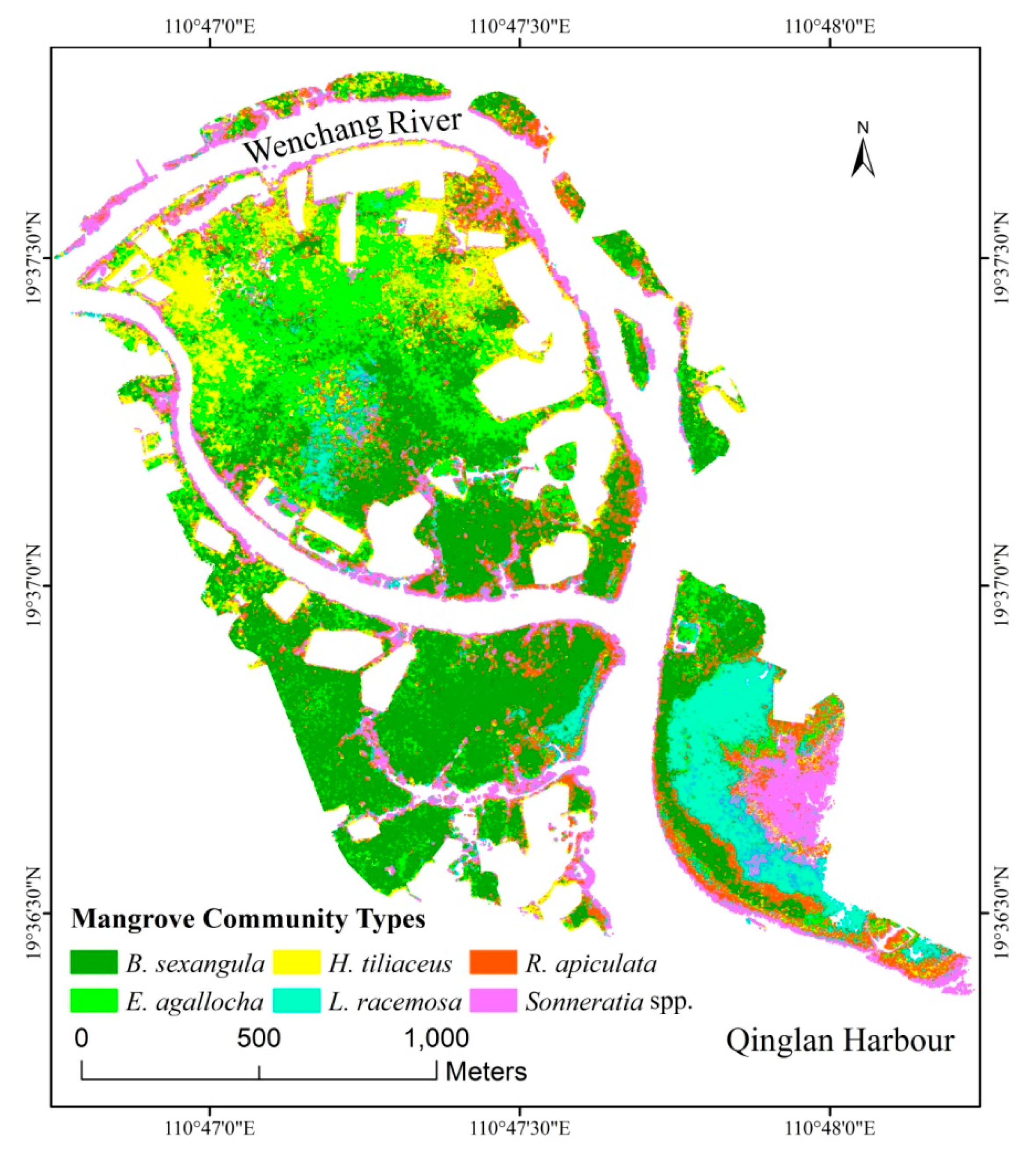
Table 6 shows the classification accuracy of mangrove species at individual tree level. Table 7 describes the characteristics of tree patches in different mangrove species in the whole study area. Figure 4 presents the thematic map of the mangrove species.
The overall classification accuracy was 86.08% with the kappa coefficient of 0.83. The majority of mangrove species could be well discriminated with the producer and user accuracies higher than 80%, except for E. agallocha and R. apiculata. The accuracies of the two species ranged from 66.27% to 74.66%.
Table 7 portrays that B. sexangula and Sonneratia spp. were the two highest mangrove species (mean height 8.00 and 7.84 m, respectively) in the study area followed by R. apiculata (mean height 6.90 m). The lowest tree species is L. racemosa. Table 7 also indicates that B. sexangula and E. agallocha covered 35.01% and 18.96% of the study area, respectively, ranking first and second. The other four species each covered approximately 10% of the study area.
3.3. AGB Estimates and Prediction
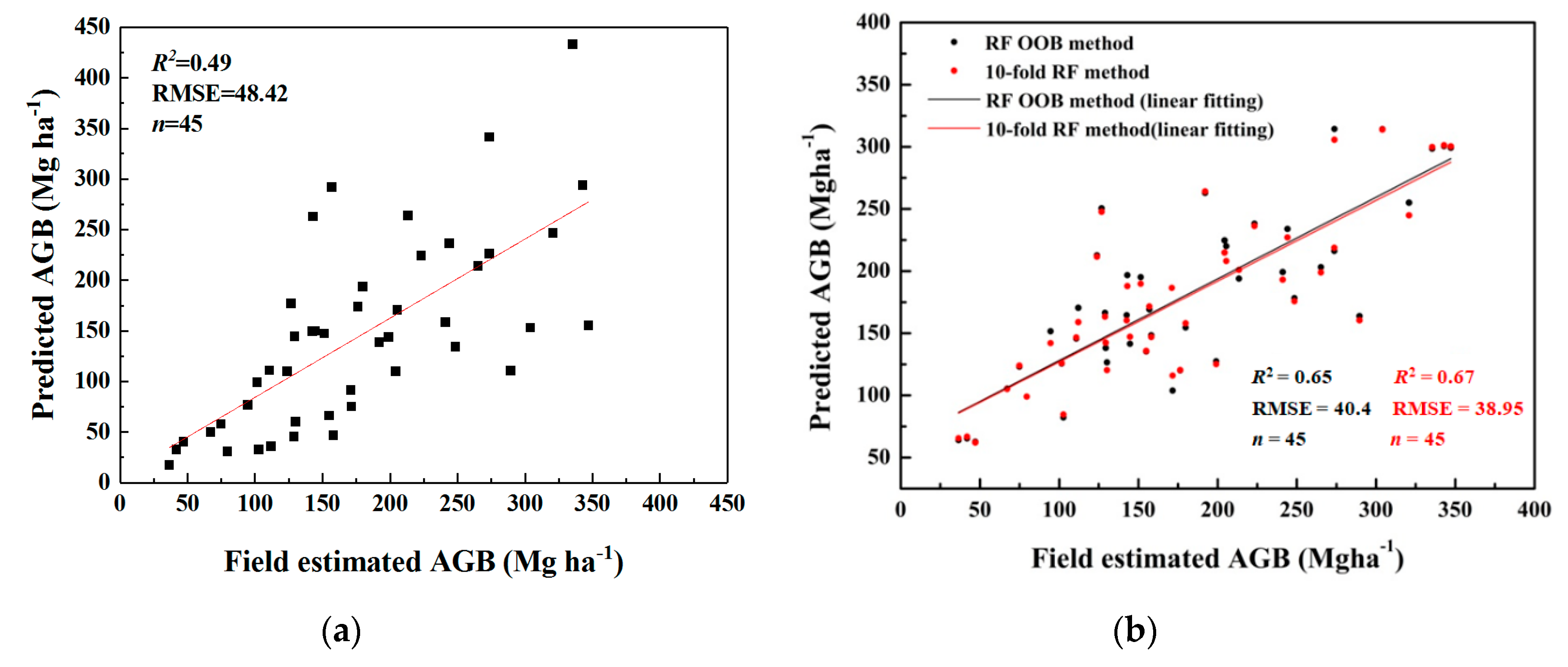
The resultant AGB density values for each species at five height levels were presented at Table 8. By applying these AGB density values to individual tree and clump, which have the species and height attributes derived from the UAV LiDAR and WorldView-2 data, the AGB of each patch and the mangrove AGB map of the study area at individual tree level could be obtained. The RF model based on 10 × 10 m grids and LiDAR metrics was used as benchmark and to predict the AGB. Figure 5 delineates the field estimated AGBs versus the predicted AGBs with the accuracy metrics.
The R2 of the individual tree-based inference method is 0.49 with an RMSE of 48.42 Mg ha−1. While, the benchmark, the grid-based RF model method, produced a higher R2 of 0.67 and a lower RMSE of 38.95 Mg ha−1. Compared with field-estimated AGB, the maximum deviation value of AGB derived from the individual tree-based inference method was 194.01 Mg·ha−1, and the minimum deviation was 1.93 Mg·ha−1. The AGB density of the whole study area calculated from the individual tree-based inference method was 119.34 Mg·ha−1, which was lower than the AGB density produced from the grid-based RF model method (148.97 Mg·ha−1). The results show that it is feasible to use the proposed individual tree-based inference method for mangrove AGB estimation in this relatively complex mangrove forest.
3.4. Spatial Distribution of Mangrove AGB
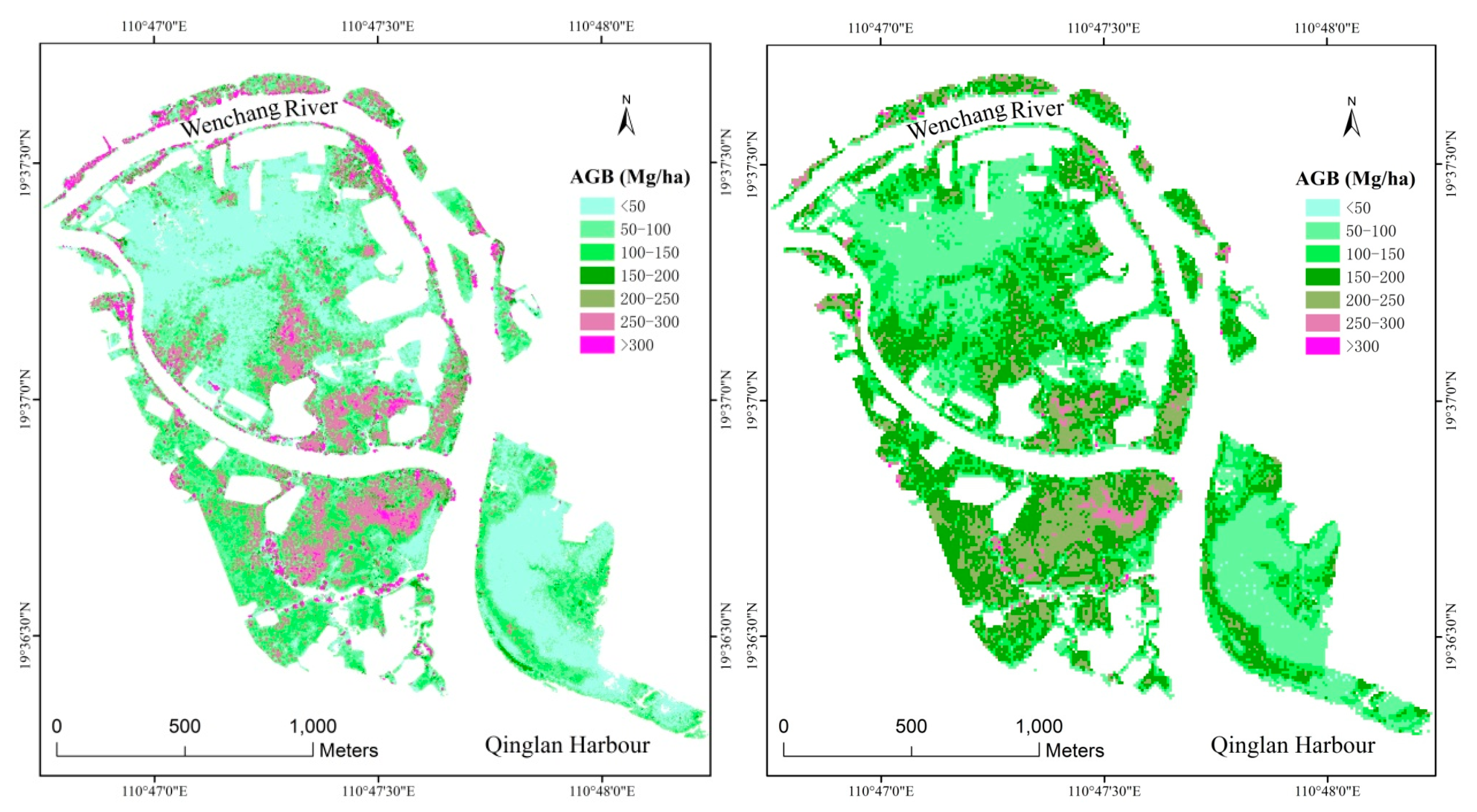
The comparison of the resultant AGB maps derived from the individual tree-based inference method and the grid-based RF model method are presented in Figure 6. According to above accuracy assessment of the two methods, the spatial distribution of the mangrove AGB in the whole study area can be better represented by the grid-based RF model method based on LiDAR metrics than the individual tree-based inference method. While, the AGB map derived from the latter method was able to portray the AGB distribution at individual tree level for each mangrove species.
The two mangrove AGB maps both show that the mangrove AGB hot spots lie in the southwest and middle of the study area, while the AGB cold spots lie in the southeast and north of the study area (Figure 6). There are also several conspicuous differences between these two maps. First, the low and middle AGB areas of the left map is overall lower than the low and middle AGB areas of the right map with one level difference. Second, the very high AGB areas (>300 Mg ha−1) are more obvious in the left map and cover larger area than those in the right map. Third, the AGB values in the left map are more heterogeneous than the AGB values in the right map.
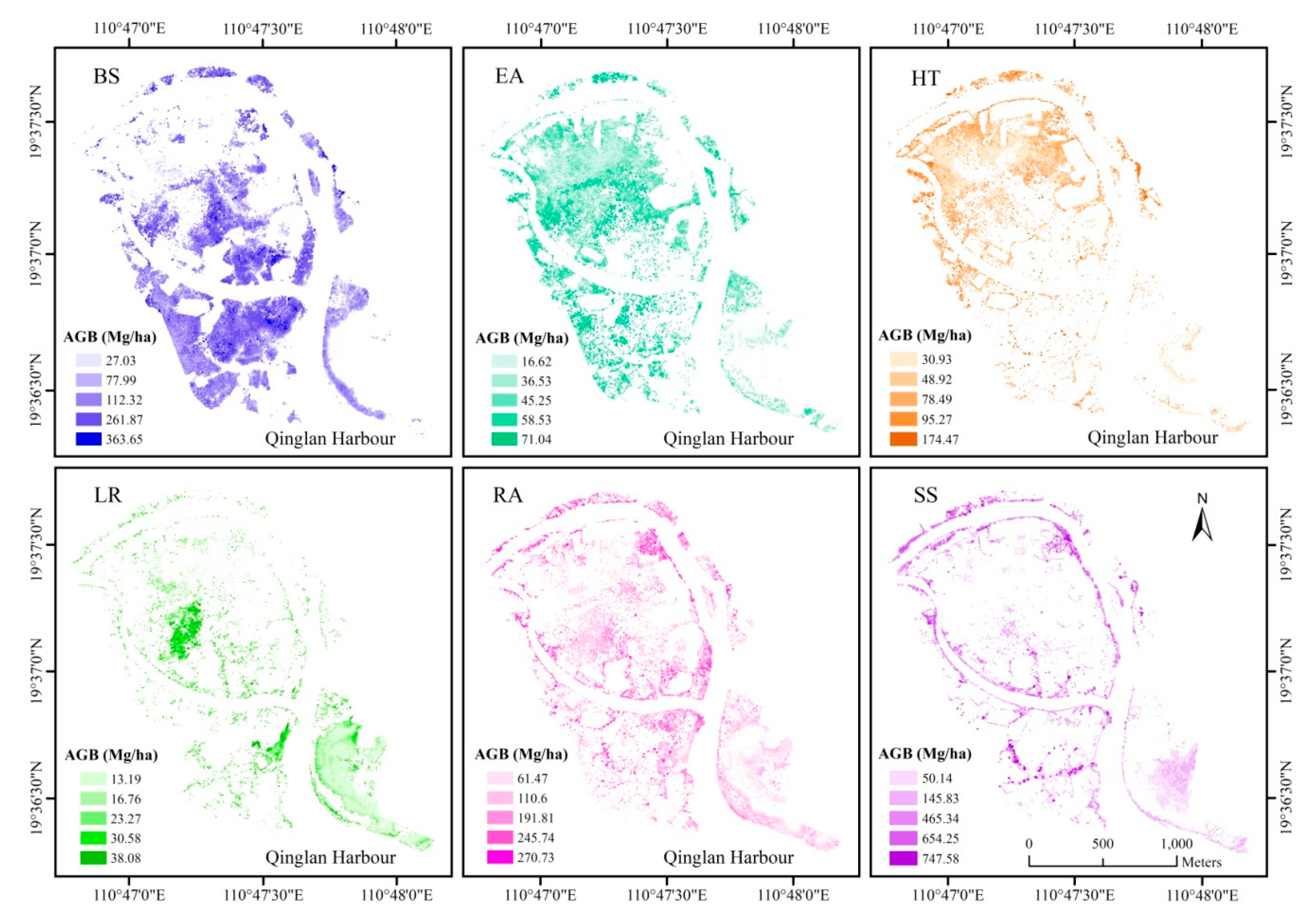
Figure 7 portrays the AGB maps of different mangrove species, which were produced by the individual tree-based inference method. The AGB of B. sexangula showed obvious concentrated distribution characteristics in space with a range of 112.32 to 363.65 Mg ha−1. E. agallocha spread out the study area with middle AGB (36.53–58.53 Mg ha−1) accounting for the largest percentage. The AGB of L. racemosa was no more than 40 Mg ha−1 due to its small individuals and represented disperse distribution. Sonneratia spp. had the largest AGB value in the study area, which was mainly distributed in fringe areas to water.
4. Discussion
4.1. Effect of Mangrove DBH on Individual Tree Segmentation
To explore the relationship between the precision of individual-tree segmentation and the size of the mangroves, the measured DBHs in 45 samples were graded in two-centimeter intervals, and the maximum, minimum, and average DBH values in each sample were determined. Then, the Pearson correlation analysis between the DBH classification and deviation of individual-tree segmentation was completed (Table A1, Appendix A).
The relationship between the DBH and the deviation was as follows: (1) The relationship between DBH and the deviation degree of individual-tree segmentation is relatively complex. Taking 14 cm as the boundary, when DBH < 14 cm, the deviation degree was negatively correlated with DBH, i.e., the deviation degree increased with the decrease in DBH. When DBH >14 cm, the deviation degree was positively correlated with DBH, and the deviation increased with the increase in DBH. This indicates that the accuracy of individual-tree segmentation decreased with the increase in DBH. When DBH < 8 cm, it was significantly negatively correlated with the DBH and the deviation, and when DBH > 30 cm, the correlation coefficient reached the maximum (0.799), it means that the accuracy of individual-tree segmentation decreased considerably. The variation of the correlation coefficient also shows that the accuracy of the segmentation number was relatively ideal within 8 cm ≤ DBH ≤ 30 cm. (2) The deviation degree has a moderate positive correlation with the maximum DBH and average DBH, but has little correlation with the minimum DBH. This means that the maximum and average DBHs are more likely to affect the accuracy of individual-tree segmentation.
4.2. Comparison of the Individual Tree-Based Inference Method and the Grid-Based RF Model Method
Concerning to AGB estimation accuracy, the grid-based RF model method was relatively higher than the individual tree-based inference method. This may be due to the fact that the former had taken fully into account and selected a large number of vegetation indicators reflecting mangrove biomass information.
In terms of mangrove AGB mapping, the grid-based RF model method can be well compared with the field AGB due to the same size of resample grids and field plots. However, whether this grid size is a more accurate AGB mapping method requires more tests and comparison of different sizes of resample grid. The individual tree-based inference method can well reflect the spatial distribution of AGB at different heights for mangrove species, and it is also more beneficial to managers to find problems. From the workflow of this study (Case 1, Figure 2) and the method Section 2.5, we could find that the proposed inference method is simple and it is easy to repeat this method in other mangrove forests or fields.
The results of the detailed comparison between the two AGB estimation methods are shown in Table 9. Although the individual tree-based inference method is considered to provide finer individual-tree information, but the current CHM-based individual tree segmentation still has insurmountable defects. For example, many lower and smaller trees are obscured by the upper tree crown and cannot be effectively identified. In addition, clump mangrove species, such as L. racemosa, cannot be well distinguished, too. These limitations inevitably reduce the accuracy of the individual-tree segmentation and then pull down the overall estimation accuracy of the AGB.
4.3. AGB Comparison with Mangroves in Other Areas
The mangroves in the study area had an AGB value of 82.088–209.520 Mg·ha−1. Compared with the mangrove AGB in other parts of the world, the AGB of B. sexangular-dominated forest is 204.933 Mg·ha−1, lower than the value of 279.00 Mg·ha−1 in Indonesia [61]. The AGB of E. agallocha-dominated forest is 82.088 Mg·ha−1, higher than the value of 14.93 Mg·ha−1 for pure E. agallocha forest in India (Central Sundarbans) [62]. The AGB of Sonneratia spp.-dominated forest is 277.201 Mg·ha−1, higher than the value of 169.61 Mg·ha−1 in India (Western Sundarbans) [62], the value of 22.30 Mg·ha−1 in China (Guangdong, Futian) [63] and the value of 189.37 Mg·ha−1 in China (Guangdong, Leizhou) [64], but lower than the value of 281.20 Mg·ha−1 in Thailand (Southern Ranong) [65]. The AGB of R. apiculata-dominated forest is 209.52 Mg·ha−1, much lower than those of both pure and mixed forests found in tropical regions (214.00 Mg·ha−1 in India (Andaman Island) [66], 216.00 Mg·ha−1 in Thailand (Chumphon Sawi Bay) [67], 298.50 Mg·ha−1 in Thailand (Ranong Southern) [65], 295.50–350.30 Mg·ha−1 in Vietnam (Mekong delta) [68], 460.00 Mg·ha−1 in Malaysia (Matang) [69], and 356.80 Mg·ha−1 in Indonesia (Halmahera) [70]).
Overall, the AGB of this study essentially aligns with the latitude law of AGB distribution in mangroves, i.e., AGB increases with the decrease in latitude.
5. Conclusions
In this study, we combined the advantages of WorldView-2, UAV LiDAR, and field survey data and proposed a novel method to estimate mangrove AGB at individual tree scale, i.e., individual tree-based inference method, and compared it with the benchmark grid-based RF model method. Although the AGB estimation accuracy of this new method is less than that of the grid-based RF inversion method (R2 of 0.49 vs. 0.67 and RMSE of 48.42 Mg ha−1 vs. 38.95 Mg ha−1), the individual tree-based inference method still has some merits. The individual tree-based inference method can show the spatial distribution details of mangrove AGB in different mangrove species, which is more beneficial to the fine management of mangroves. Considering that the mangrove forest in the study area is complex, the results of the newly proposed method are relatively satisfying.
There are many uncertainties in mangrove AGB estimation due to sampling type, spatial resolution of remote sensing data, local topography, biophysical conditions, forest structure, wood density, tree species, size of trees, selection of allometric models, and technical factors related to data processing. Traditional field surveys are still the most important base for establishing a reliable relationship between biomass and remote sensing variables. With the support of a variety of remote sensing data, more targeted field survey methods, such as tree species, habitat, forest age and wood density, will be further tried.
Author Contributions
Conceptualization, P.Q., D.W. and X.Z.; Methodology, P.Q. and D.W.; Software, P.Q. and D.W.; Validation, P.Q. and D.W.; Formal analysis, P.Q. and D.W.; Investigation, P.Q., D.W., X.Y., G.X. and Z.Z.; Resources, P.Q.; Data curation, P.Q.; Writing—original draft preparation, P.Q.; Writing—review & editing, P.Q., D.W., X.Z. and X.Y.; Visualization, P.Q. and D.W.; Supervision, D.W.; Project administration, P.Q. and S.X.; Funding acquisition, P.Q. and S.X.
Funding
National Natural Science Foundation of China: 41361090, 41877411. This research received no external funding.
Acknowledgments
Authors are thankful to the Administration Station of Qinglan Harbor Mangrove Nature Reserve for providing maps of the Nature Reserve. This study is supported by the National Natural Science Foundation of China (No. 41361090, 41877411).
Conflicts of Interest
The authors declare no conflict of interest.
Appendix A

Table A1.
Pearson correlation analysis of diameter at breast height (DBH) classification and deviation of individual-tree segmentation measured in two-centimeter intervals.
Table A1.
Pearson correlation analysis of diameter at breast height (DBH) classification and deviation of individual-tree segmentation measured in two-centimeter intervals.
| DBH1 | DBH2 | DBH3 | DBH4 | DBH5 | DBH6 | DBH7 | DBH8 | DBH9 | DBH10 | DBH11 | DBH12 | DBH13 | DBH14 | DBH15 | DBH16 | DBH17 | DBH18 | DBH19 | DBH20 | DBH21 | Max. | Min. | Mean | |
|---|---|---|---|---|---|---|---|---|---|---|---|---|---|---|---|---|---|---|---|---|---|---|---|---|
| DBH1 | 1 | |||||||||||||||||||||||
| DBH2 | 0.094 | 1 | ||||||||||||||||||||||
| DBH3 | 0.078 | 0.173 | 1 | |||||||||||||||||||||
| DBH4 | 0.157 | −0.244 | 0.258 | 1 | ||||||||||||||||||||
| DBH5 | −0.002 | −.202 | 0.258 | 0.834 ** | 1 | |||||||||||||||||||
| DBH6 | 0.243 | −0.213 | 0.146 | 0.804 ** | 0.814 ** | 1 | ||||||||||||||||||
| DBH7 | 0.292 | −0.374 * | −0.154 | 0.611 ** | 0.541 ** | 0.676 ** | 1 | |||||||||||||||||
| DBH8 | 0.084 | −0.276 | −0.275 | 0.262 | 0.226 | 0.469 ** | 0.604 ** | 1 | ||||||||||||||||
| DBH9 | 0.086 | −0.248 | −0.208 | 0.323 * | 0.304 * | 0.523 ** | 0.576 ** | 0.535 ** | 1 | |||||||||||||||
| DBH10 | −0.044 | −0.064 | −0.306 * | −0.045 | 0.072 | 0.152 | 0.338 * | 0.568 ** | 0.489 ** | 1 | ||||||||||||||
| DBH11 | −0.034 | −0.097 | −0.124 | 0.197 | 0.289 | 0.400 ** | 0.475 ** | 0.315 * | 0.608 ** | 0.347 * | 1 | |||||||||||||
| DBH12 | −0.056 | 0.084 | −0.284 | −0.145 | −0.085 | 0.074 | 0.124 | 0.241 | 0.509 ** | 0.508 ** | 0.617 ** | 1 | ||||||||||||
| DBH13 | −0.074 | −0.164 | −0.268 | −0.266 | −0.131 | −0.158 | 0.003 | 0.117 | 0.184 | 0.147 | 0.295 * | 0.141 | 1 | |||||||||||
| DBH14 | 0.087 | −0.016 | −0.249 | −0.265 | −0.154 | −0.083 | −0.052 | 0.328 * | 0.381 ** | 0.442 ** | 0.275 | 0.390 ** | 0.624 ** | 1 | ||||||||||
| DBH15 | −0.094 | 0.075 | −0.211 | −0.085 | −0.049 | −0.023 | 0.008 | −0.037 | 0.217 | 0.088 | 0.485 ** | 0.531 ** | 0.609 ** | 0.345 * | 1 | |||||||||
| DBH16 | −0.081 | −0.147 | −0.197 | −0.229 | −0.115 | −0.149 | −0.020 | −0.026 | 0.019 | −0.043 | 0.286 | 0.146 | 0.835 ** | 0.393 ** | 0.659 ** | 1 | ||||||||
| DBH17 | 0.087 | −0.045 | −0.053 | −0.142 | −0.028 | 0.018 | −0.004 | −0.036 | 0.036 | −0.040 | 0.334 * | 0.106 | 0.823 ** | 0.347 * | 0.623 ** | 0.831 ** | 1 | |||||||
| DBH18 | 0.008 | −0.098 | −0.188 | −0.147 | −0.060 | 0.026 | 0.039 | 0.181 | 0.551 ** | 0.234 | 0.405 ** | 0.357 * | 0.687 ** | 0.791 ** | 0.402 ** | 0.376 * | 0.464 ** | 1 | ||||||
| DBH19 | −0.056 | −0.105 | −0.119 | −0.081 | −0.040 | −0.008 | 0.056 | 0.221 | 0.294 * | 0.109 | 0.200 | 0.145 | 0.499 ** | 0.543 ** | 0.096 | 0.139 | 0.218 | 0.764 ** | 1 | |||||
| DBH20 | −0.066 | −0.103 | −0.058 | −0.058 | 0.042 | 0.062 | 0.059 | 0.102 | −0.031 | 0.079 | 0.298 * | −0.016 | 0.170 | 0.117 | 0.056 | 0.408 ** | 0.159 | −0.058 | −0.044 | 1 | ||||
| DBH21 | −0.039 | −0.079 | −0.097 | −0.134 | −0.066 | −0.031 | −0.017 | 0.102 | 0.383 ** | 0.132 | 0.269 | 0.201 | 0.522 ** | 0.628 ** | 0.133 | 0.176 | 0.262 | 0.866 ** | 0.892 ** | −0.033 | 1 | |||
| Max. | 0.126 | −0.294 | −0.320 * | 0.130 | 0.207 | 0.393 ** | 0.465 ** | 0.574 ** | 0.528 ** | 0.462 ** | 0.622 ** | 0.519 ** | 0.518 ** | 0.532 ** | 0.469 ** | 0.463 ** | 0.422 ** | 0.467 ** | 0.382 ** | 0.379 * | 0.307 * | 1 | ||
| Min. | −0.306 * | −0.120 | −0.162 | 0.031 | −0.001 | −0.090 | 0.140 | −0.012 | −0.155 | −0.076 | 0.006 | −0.110 | 0.001 | −0.241 | 0.156 | 0.092 | −0.031 | −0.251 | −0.215 | 0.038 | −0.265 | −0.159 | 1 | |
| Mean | −0.005 | −0.250 | −0.518 ** | −0.151 | −0.037 | 0.040 | 0.260 | 0.372 * | 0.412 ** | 0.488 ** | 0.487 ** | 0.565 ** | 0.692 ** | 0.628 ** | 0.660 ** | 0.634 ** | 0.483 ** | 0.493 ** | 0.296 * | 0.306 * | 0.309 * | 0.791 ** | 0.142 | 1 |
| DA | −0.211 | −0.356 * | −0.388 ** | −0.116 | −0.024 | −0.002 | 0.302 * | 0.309 * | 0.371 * | 0.289 | 0.360 * | 0.226 | 0.799 ** | 0.394 ** | 0.569 ** | 0.637 ** | 0.603 ** | 0.522 ** | 0.395 ** | 0.054 | 0.391 ** | 0.556 ** | 0.086 | 0.695 ** |
DBH1, DBH2, DBH20, DBH21 denote DBH < 4 cm, 4 ≤ DBH < 6cm, 40 ≤ DBH < 42 cm, DBH ≥ 42 cm, respectively; Max. means maximum DBH, Min. means minimum DBH; * Significant at 5%; ** Significant at 1%.
References
- Saenger, P. Mangrove Ecology, Silviculture and Conservation; Kluwer Academic: Dordrecht, The Nederlands, 2003. [Google Scholar]
- Constanza, R.; d’Arge, R.; de Groot, R.; Farber, S.; Grasso, M.; Hannon, B.; Limberg, K.; Naeem, S.; O’Neill, R.V.; Paruelo, J.; et al. The value of the world’s ecosystem service and natural capital. Ecol. Econ. 1997, 25, 3–15. [Google Scholar] [CrossRef]
- Donato, D.C.; Kauffman, J.B.; Murdiyarso, D.; Kurnianto, S.; Stidham, M.; Kanninen, M. Mangroves among the most carbon–rich forests in the tropics. Nat. Geosci. 2011, 4, 293–297. [Google Scholar] [CrossRef]
- Barbier, E.B.; Hacker, S.D.; Kennedy, C.; Koch, E.W.; Stier, A.C.; Silliman, B.R. The value of estuarine and coastal ecosystem services. Ecol. Monogr. 2011, 81, 169–193. [Google Scholar] [CrossRef]
- Hickey, S.M.; Callow, N.J.; Phinn, S.; Lovelock, C.E.; Duarte, C.M. Spatial complexities in aboveground carbon stocks of a semi–arid mangrove community: A remote sensing height–biomass–carbon approach. Estuar. Coast. Shelf Sci. 2018, 200, 194–201. [Google Scholar] [CrossRef]
- Giri, C.; Ochieng, E.; Tieszen, L.L.; Zhu, Z.; Singh, A.; Loveland, T.; Masek, J.; Duke, N. Status and distribution of mangrove forests of the world using earth observation satellite data. Glob. Ecol. Biogeogr. 2011, 20, 154–159. [Google Scholar] [CrossRef]
- Hamilton, S.E.; Friess, D.A. Global carbon stocks and potential emissions due to mangrove deforestation from 2000 to 2012. Nat. Clim. Chang. 2018, 8, 240–244. [Google Scholar] [CrossRef] [Green Version]
- Fehrmann, L.; Kleinn, C. General considerations about the use of allometric equations for biomass estimation on the example of Norway spruce in central Europe. Ecol. Manag. 2006, 236, 412–421. [Google Scholar] [CrossRef]
- Komiyama, A.; Ong, J.E.; Poungparn, S. Allometry, biomass, and productivity of mangrove forests: A review. Aquat. Bot. 2008, 8, 128–137. [Google Scholar] [CrossRef]
- Ketterings, Q.M.; Coe, R.; van Noordwijk, M.; Ambagu, Y.; Palm, C.A. Reducing uncertainty in use of allometric biomass equations for predicting above–ground tree biomass in mixed secondary forests. Ecol. Manag. 2001, 146, 199–202. [Google Scholar] [CrossRef]
- Overman, J.P.M.; Witte, H.J.L.; Saldarriaga, J.G. Evaluation of regression models for above–ground biomass determination in Amazon rainforest. J. Trop. Ecol. 1994, 10, 207–218. [Google Scholar] [CrossRef]
- Proisy, C.; Couteron, P.; Fromard, F. Predicting and mapping mangrove biomass from canopy grain analysis using Fourier–based textural ordination of IKONOS images. Remote Sens. Environ. 2007, 109, 379–392. [Google Scholar] [CrossRef]
- Jachowski, N.R.A.; Quak, M.S.Y.; Friess, D.A.; Duangnamon, D.; Webb, E.; Ziegler, A.D. Mangrove biomass estimation in Southwest Thailand using machine learning. Appl. Geogr. 2013, 45, 311–321. [Google Scholar] [CrossRef]
- Hamdan, O.; Aziz, H.K.; Hasmadi, I.M. L–band ALOS PALSAR for biomass estimation of Matang Mangroves, Malaysia. Remote Sens. Environ. 2014, 155, 69–78. [Google Scholar] [CrossRef]
- Hartoko, A.; Chayaningrum, S.; Febrianti, D.A.; Ariyanto, D. Carbon biomass algorithms development for mangrove vegetation in Kemujan, Parang Island Karimunjawa National Park and Demak Coastal Area—Indonesia. Procedia Environ. Sci. 2015, 23, 39–47. [Google Scholar] [CrossRef]
- Aslan, A.; Rahman, A.F.; Warren, M.W.; Robeson, S.M. Mapping spatial distribution and biomass of coastal wetland vegetation in Indonesian Papua by combining active and passive remotely sensed data. Remote Sens. Environ. 2016, 183, 65–81. [Google Scholar] [CrossRef]
- Castillo, J.A.A.; Apan, A.A.; Maraseni, T.N.; Salmo, S.G., III. Estimation and mapping of above–ground biomass of mangrove forests and their replacement land uses in the Philippines using Sentinel imagery. ISPRS J. Photogramm. Remote Sens. 2017, 134, 70–85. [Google Scholar] [CrossRef]
- Pham, L.T.H.; Brabyn, L. Monitoring mangrove biomass change in Vietnam using SPOT images and an object–based approach combined with machine learning algorithms. ISPRS J. Photogramm. Remote Sens. 2017, 128, 86–97. [Google Scholar] [CrossRef]
- Dalponte, M.; Frizzera, L.; Ørka, H.O.; Gobakken, T.; Næsset, E.; Gianelle, D. Predicting stem diameters and aboveground biomass of individual trees using remote sensing data. Ecol. Indic. 2018, 85, 367–376. [Google Scholar] [CrossRef]
- Owers, C.J.; Rogers, K.; Woodroffe, C.D. Terrestrial laser scanning to quantify above–ground biomass of structurally complex coastal wetland vegetation. Estuar. Coast. Shelf Sci. 2018, 204, 164–176. [Google Scholar] [CrossRef]
- Demir, N. Using UAVs for detection of trees from digital surface models. J. For. Res. 2018, 29, 813–821. [Google Scholar] [CrossRef]
- Kestur, R.; Angural, A.; Bashir, B.; Omkar, S.N.; Anand, G.; Meenavathi, M.B. Tree Crown Detection, Delineation and Counting in UAV Remote Sensed Images: A Neural Network Based Spectral–Spatial Method. J. Indian Soc. Remote Sens. 2018, 46, 991–1004. [Google Scholar] [CrossRef]
- Disney, M.; Burt, A.; Calders, K.; Schaaf, C.; Stovall, A. Innovations in ground and airborne technologies as reference and for training and validation: Terrestrial laser scanning (TLS). Surv. Geophys. 2019. [Google Scholar] [CrossRef]
- Kędra, K.; Barbeito, I.; Dassot, M.; Vallet, P.; Gazda, A. Single–image photogrammetry for deriving tree architectural traits in mature forest stands: A comparison with terrestrial laser scanning. Ann. For. Sci. 2019, 76, 5. [Google Scholar] [CrossRef]
- Carrijo, J.V.N.; de Freitas Ferreira, A.B.; Ferreira, M.C.; de Aguiar, M.C.; Miguel, E.P.; Matricardi, E.A.T.; Rezende, A.V. The growth and production modeling of individual trees of Eucalyptus urophylla plantations. J. For. Res. 2019. [Google Scholar] [CrossRef]
- Yin, D.; Wang, L. Individual mangrove tree measurement using UAV–based LiDAR data: Possibilities and challenges. Remote Sens. Environ. 2019, 223, 34–49. [Google Scholar] [CrossRef]
- Shao, Z.F.; Zhang, L.J.; Wang, L. Stacked sparse autoencoder modeling using the synergy of airborne LiDAR and satellite optical and SAR data to map forest above-ground biomass. IEEE J. Sel. Top. Appl. Earth Obs. Remote Sens. 2017, 10, 5569–5582. [Google Scholar] [CrossRef]
- Baral, S. Mapping Carbon Stock Using High Resolution Satellite Images in Sub–Tropical Forest of Nepal; University of Twente University of Faculty of Geo-Information and Earth Observation (ITC): Enschede, The Netherlands, 2011. [Google Scholar]
- Maharjan, S. Estimation and Mapping above Ground Woody Carbon Stocks Using LiDAR Data and Digital Camera Imagery in the Hilly Forests of Gorkha, Nepal; University of Twente University of Faculty of Geo-Information and Earth Observation (ITC): Enschede, The Netherlands, 2012. [Google Scholar]
- Karna, Y.K.; Hussin, Y.A.; Gilani, H.; Bronsveld, M.C.; Murthy, M.S.R.; Qamer, F.M.; Karky, B.S.; Bhattarai, T.; Aigong, X.; Baniya, C.B. Integration of WorldView–2 and airborne LiDAR data for tree species level carbon stock mapping in Kayar Khola watershed, Nepal. Int. J. Appl. Earth Obs. Geoinf. 2015, 38, 280–291. [Google Scholar] [CrossRef]
- Zhang, L.; Shao, Z.; Liu, J.; Cheng, Q. Deep learning based retrieval of forest aboveground biomass from combined lidar and landsat 8 data. Remote Sens. 2019, 11, 1459. [Google Scholar] [CrossRef]
- Nandy, S.; Ghosh, S.; Kushwaha, S.P.S.; Kumar, A.S. Remote sensing–based forest biomass assessment in northwest Himalayan landscape. In Remote Sensing of Northwest Himalayan Ecosystems; Navalgund, R.R., Kumar, A.S., Nandy, S., Eds.; Springer: Singapore, 2019. [Google Scholar]
- Meyer, V.; Saatchi, S.; Ferraz, A.; Xu, L.; Duque, A.; García, M.; Chave, J. Forest degradation and biomass loss along the Chocó region of Colombia. Carbon Balance Manag. 2019, 14, 2. [Google Scholar] [CrossRef]
- Kellner, J.R.; Armston, J.; Birrer, M.; Cushman, K.C.; Duncanson, L.; Eck, C.; Falleger, C.; Imbach, B.; Král, K.; Krůček, M.; et al. New Opportunities for Forest Remote Sensing Through Ultra High Density Drone LiDAR. Surv. Geophys. 2019. [Google Scholar] [CrossRef]
- Hamilton, S.E.; Castellanos–Galindo, G.A.; Millones–Mayer, M.; Chen, M. Remote sensing of mangrove forests: Current techniques and existing databases. In Threats to Mangrove Forests; Makowski, C., Finkl, C.W., Eds.; Coastal Research Library: Boca Raton, FL, USA, 2018; Volume 25, pp. 497–520. [Google Scholar]
- Fragoso–Campón, L.; Quirós, E.; Mora, J.; Gallego, J.A.G.; Durán–Barroso, P. Overstory–understory land cover mapping at the watershed scale: Accuracy enhancement by multitemporal remote sensing analysis and LiDAR. Environ. Sci. Pollut. Res. 2019. [Google Scholar] [CrossRef] [PubMed]
- Cintron, G.; Schaeffer–Novelli, S.Y. Methods for studying Mangrove structure. In The Mangrove Ecosystems: Research Methods; Snedaker, S.C., Snedaker, J., Eds.; UNESCO: Paris, France, 1984; pp. 91–113. [Google Scholar]
- Clough, B.F.; Scott, K. Allometric relationships for estimating above–ground biomass in six mangrove species. For. Ecol. Manag. 1989, 27, 117–127. [Google Scholar] [CrossRef]
- Hossain, M.; Siddique, M.R.H.; Saha, S.; Abdullah, S.M.R. Allometric models for biomass, nutrients and carbon stock in Excoecaria agallocha of the Sundarbans, Bangladesh. Wetl. Ecol. Manag. 2015, 23, 765–774. [Google Scholar] [CrossRef]
- Ong, J.E.; Gong, W.K.; Wong, C.H. Allometry and partitioning of the mangrove, Rhizophora apiculata. For. Ecol. Manag. 2004, 188, 395–408. [Google Scholar] [CrossRef]
- Fromard, F.; Puig, H.; Mougin, E.; Marty, G.; Betoulle, J.L.; Cadamuro, L. Structure of above–ground biomass and dynamics of mangrove ecosystems: New data from French Guiana. Oecologia 1998, 115, 39–53. [Google Scholar] [CrossRef]
- Tam, N.F.Y.; Wong, Y.S.; Lan, C.Y.; Chen, G.Z. Community structure and standing crop biomass of a mangrove forest in Futian Nature Reserve, Shenzhen, China. Hydrobiologia 1995, 295, 193–201. [Google Scholar] [CrossRef]
- Kusmana, C.; Hidayat, T.; Tiryana, T.; Rusdiana, O. Allometric models for above-and below–ground biomass of Sonneratia spp. Glob. Ecol. Conserv. 2018, 15, e00417. [Google Scholar] [CrossRef]
- Komiyama, A.; Poungparn, S.; Kato, S. Common allometric equations for estimating the tree weight of mangroves. J. Trop. Ecol. 2005, 21, 471–477. [Google Scholar] [CrossRef]
- Wang, D.; Wan, B.; Qiu, P.; Su, Y.; Guo, Q.; Wang, R.; Sun, F.; Wu, X. Evaluating the Performance of Sentinel-2, Landsat 8 and Pléiades-1 in Mapping Mangrove Extent and Species. Remote Sens. 2018, 10, 1468. [Google Scholar] [CrossRef]
- Breiman, L. Random Forests. Mach. Learn. 2001, 45, 5–32. [Google Scholar] [CrossRef] [Green Version]
- Leboeuf, A.; Beaudoin, A.; Fournier, R.A.; Guindon, L.; Luther, J.E.; Lambert, M.-C. A shadow fraction method for mapping biomass of northern boreal black spruce forests using QuickBird imagery. Remote Sens. Environ. 2007, 110, 488–500. [Google Scholar] [CrossRef]
- Holmgren, J.; Persson, A.; Söderman, U. Species identification of individual trees by combining high resolution LiDAR data with multi–spectral images. Int. J. Remote Sens. 2008, 29, 1537–1552. [Google Scholar] [CrossRef]
- Othmani, A.; Piboule, A.; Krebs, M.; Stolz, C.; Voon, L.L.Y. Towards automated and operational forest inventories with T–LiDAR. In Proceedings of the 11th International Conference on LiDAR Applications for Assessing Forest Ecosystems (SilviLaser 2011), Hobart, Australia, 16–20 October 2011. [Google Scholar]
- Sousa, A.M.O.; Gonçalves, A.C.; Mesquita, P.; da Silva, J.R.M. Biomass estimation with high resolution satellite images: A case study of Quercus rotundifolia. ISPRS J. Photogramm. Remote Sens. 2015, 101, 69–79. [Google Scholar] [CrossRef] [Green Version]
- Aihua Li Glenn, N.F.; Olsoy, P.J.; Mitchell, J.J.; Shrestha, R. Aboveground biomass estimates of sagebrush using terrestrial and airborne LiDAR data in a dryland ecosystem. Agric. For. Meteorol. 2015, 213, 138–147. [Google Scholar]
- Dalponte, M.; Coomes, D.A. Tree–centric mapping of forest carbon density from airborne laser scanning and hyperspectral data. Methods Ecol. Evol. 2016, 7, 1236–1245. [Google Scholar] [CrossRef]
- Stovall, A.E.L.; Anderson–Teixeira, K.J.; Shugart, H.H. Assessing terrestrial laser scanning for developing non–destructive biomass allometry. For. Ecol. Manag. 2018, 427, 217–229. [Google Scholar] [CrossRef]
- Bazezew, M.N.; Hussin, Y.A.; Kloosterman, E.H. Integrating airborne LiDAR and terrestrial laser scanner forest parameters for accurate above–ground biomass/carbon estimation in Ayer Hitam tropical forest, Malaysia. Int. J. Appl. Earth Obs. Geoinf. 2018, 73, 638–652. [Google Scholar] [CrossRef]
- Wang, L.; Gong, P.; Biging, G.S. Individual tree–crown delineation and treetop detection in high–spatial–resolution aerial imagery. Photogramm. Eng. Remote Sens. 2004, 70, 351–357. [Google Scholar] [CrossRef]
- Duro, D.C.; Franklin, S.E.; Dubé, M.G. A comparison of pixel-based and object-based image analysis with selected machine learning algorithms for the classification of agricultural landscapes using SPOT-5 HRG imagery. Remote Sens. Environ. 2012, 118, 259–272. [Google Scholar] [CrossRef]
- Yin, D.; Wang, L. How to assess the accuracy of the individual tree-based forest inventory derived from remotely sensed data: A review. Int. J. Remote Sens. 2016, 37, 4521–4553. [Google Scholar] [CrossRef]
- Strîmbu, V.F.; Strîmbu, B.M. A graph-based segmentation algorithm for tree crown extraction using airborne LiDAR data. ISPRS J. Photogramm. Remote Sens. 2015, 104, 30–43. [Google Scholar] [CrossRef] [Green Version]
- Zhou, T.; Popescu, S.; Lawing, A.; Eriksson, M.; Strimbu, B.; Bürkner, P. Bayesian and classical machine learning methods: A comparison for tree species classification with LiDAR waveform signatures. Remote Sens. 2018, 10, 39. [Google Scholar] [CrossRef]
- Pouliot, D.A.; King, D.J.; Bell, F.W.; Pitt, D.G. Automated tree crown detection and delineation in high-resolution digital camera imagery of coniferous forest regeneration. Remote Sens. Environ. 2002, 82, 322–334. [Google Scholar] [CrossRef]
- Kusmana, C.; Sabiham, S.; Abe, K.; Watanabe, H. An estimation of above ground tree biomass of a mangrove forest in East Sumatra, Indonesia. Tropics. 1992, 1, 243–257. [Google Scholar] [CrossRef]
- Mitra, A.; Zaman, S. Abiotic Variables of the Marine and Estuarine Ecosystems. In Basics of Marine and Estuarine Ecology; Mitra, A., Zaman, S., Eds.; Springer: New Delhi, India, 2016; pp. 182–184. [Google Scholar]
- Zan, Q.J.; Wang, Y.J.; Liao, B.W.; Zheng, D.Z. Biomass and net productivity of Sonneratia apetala, S. caseolaris mangrove man-made forest. J. Wuhan Bot. Res. 2001, 19, 391–396. [Google Scholar]
- Han, W.D.; Gao, X.M.; Teunissen, E. Study on Sonneratia apetala productivity in restored forests in Leizhou Peninsula, China. J. For. Res. 2001, 12, 229–234. [Google Scholar]
- Komiyama, A.; Ogino, K.; Aksomkoae, S.; Sabhasri, S. Root biomass of a mangrove forest in southern Thailand 1: Estimation by the trench method and the zonal structure of root biomass. J. Trop. Ecol. 1987, 3, 97–108. [Google Scholar] [CrossRef]
- Mall, L.P.; Singh, V.P.; Garge, A. Study of biomass, litter fall, litter decomposition and soil respiration in monogeneric mangrove and mixed mangrove forests of Andaman Islands. Trop. Ecol. 1991, 32, 144–152. [Google Scholar]
- Alongi, D.M.; Dixon, P. Mangrove primary production and above and below–Ground biomass in Sawi Bay, southern Thailand. Phuket Mar. Biol. Cent. Spec. Publ. 2000, 22, 31–38. [Google Scholar]
- Phan, S.M.; Nguyen, H.T.T.; Nguyen, T.K.; Lovelock, C. Modelling above ground biomass accumulation of mangrove plantations in Vietnam. For. Ecol. Manag. 2019, 432, 376–386. [Google Scholar] [CrossRef]
- Putz, F.; Chan, H.T. Tree growth, dynamics, and productivity in a mature mangrove forest in Malaysia. For. Ecol. Manag. 1986, 17, 211–230. [Google Scholar] [CrossRef]
- Komiyama, A.; Moriya, H.; Prawiroatmodjo, S.; Toma, T.; Ogino, K. Forest primary productivity. In Biological System of Mangrove; Ogino, K., Chihara, M., Eds.; Ehime University: Matsuyama, Japan, 1988; pp. 97–117. [Google Scholar]
Figure 1.
Location of the study area and the sampling plots.

Figure 2.
Workflow of estimating mangrove aboveground biomass (AGB). Case 1 denotes the mangrove AGB estimation at individual tree level, namely the individual tree-based inference method. Case 2 denotes the common model-based AGB estimation at grid level, namely the grid-based random forest model method, which is used as a benchmark in this study.

Figure 3.
Spectral curves of different mangrove species.

Figure 4.
Classification and distribution map of mangroves in the study area.

Figure 5.
Accuracy comparison of AGB between the field estimated and predicted values. (a): Case 1, individual tree-based inference method. (b): Case 2, grid-based RF model method.
Figure 5.
Accuracy comparison of AGB between the field estimated and predicted values. (a): Case 1, individual tree-based inference method. (b): Case 2, grid-based RF model method.

Figure 6.
AGB distribution maps of the study area produced from individual tree-based inference method (left) and the grid-based random forest (RF) model method (right).
Figure 6.
AGB distribution maps of the study area produced from individual tree-based inference method (left) and the grid-based random forest (RF) model method (right).

Figure 7.
AGB distribution maps in different mangrove species determined from the individual tree-based inference method. BS: B. sexangula; EA: E. agallocha; HT: H. tiliaceus; LR: L. racemosa; RA: R. apiculata; SS: Sonneratia spp.
Figure 7.
AGB distribution maps in different mangrove species determined from the individual tree-based inference method. BS: B. sexangula; EA: E. agallocha; HT: H. tiliaceus; LR: L. racemosa; RA: R. apiculata; SS: Sonneratia spp.

Table 1.
Summary of the community structure of the mangrove forest in 45 sample plots.
| Species | Count | Density (Individuals·100 m−2) | RD (%) | F (%) | ReF (%) | BA (m2) | Dominance (m2 ha−1) | RDo (%) | IVI |
|---|---|---|---|---|---|---|---|---|---|
| B. sexangula | 1063 | 8.93 | 27.74 | 67.31 | 20.02 | 16.514 | 13.877 | 46.75 | 31.50 |
| E. agallocha | 694 | 5.83 | 18.11 | 71.11 | 21.15 | 4.462 | 3.750 | 12.63 | 17.30 |
| H. tiliaceus | 250 | 2.10 | 6.53 | 35.56 | 10.58 | 1.371 | 1.152 | 3.88 | 7.00 |
| H. littoralis | 18 | 0.15 | 0.47 | 4.44 | 1.32 | 1.187 | 0.997 | 3.36 | 1.72 |
| X. granatum | 98 | 0.82 | 2.56 | 31.11 | 9.25 | 0.887 | 0.745 | 2.51 | 4.77 |
| R. apiculata | 402 | 3.38 | 10.49 | 35.56 | 10.58 | 3.938 | 3.309 | 11.15 | 10.74 |
| A. corniculatum | 469 | 3.94 | 12.24 | 8.89 | 2.64 | 0.655 | 0.550 | 1.85 | 5.58 |
| K. candel | 4 | 0.03 | 0.10 | 6.67 | 1.98 | 0.009 | 0.007 | 0.03 | 0.70 |
| L. racemosa | 543 | 4.56 | 14.17 | 28.89 | 8.59 | 1.516 | 1.274 | 4.29 | 9.02 |
| C. tagal | 112 | 0.94 | 2.92 | 2.22 | 0.66 | 0.213 | 0.179 | 0.60 | 1.39 |
| S. ovata | 50 | 0.42 | 1.31 | 13.33 | 3.97 | 1.453 | 1.221 | 4.12 | 3.13 |
| S. apetala | 48 | 0.40 | 1.25 | 13.33 | 3.97 | 1.859 | 1.562 | 5.26 | 3.49 |
| S. alba | 81 | 0.68 | 2.11 | 17.78 | 5.29 | 1.259 | 1.058 | 3.57 | 3.66 |
| Total | 3832 | 32.20 | 100.00 | 336.20 | 100.00 | 35.322 | 29.682 | 100.00 | 100.00 |
BA is basal area, BA = ∑(DBH2 × π)/(4 × 10,000); RD is relative density; F is frequency, which calculated as: F = number of sample plots occurring in some kind of plant/total number of sample plots × 100; ReF is relative frequency; RDo is relative dominance; IVI is importance value index, IVI = (relative density + relative frequency + relative dominance)/3 [37].
Table 2.
Allometric equations for mangrove species used in this study.
| No. | Species | Allometric Equations | References |
|---|---|---|---|
| 1 | B. sexangula | AGB = 0.168 × DBH2.42 | [38] |
| 2 | E. agallocha | LogAGB = 1.0996 × logDBH2 − 0.8572 | [39] |
| 3 | R. apiculata | AGB = 0.235 × DBH2.420 | [40] |
| 4 | C. tagal | AGB = 0.1885 × DBH2.3379 | [38] |
| 5 | L. racemosa | AGB = 0.1023 × DBH2.50 | [41] |
| 6 | A. corniculatum | LogAGB = 1.496 + 0.465 × log (DBH2 × H) | [42] |
| 7 | X. granatum | AGB = 0.0823 × DBH2.5883 | [38] |
| 8 | K. candel | LogAGB = 2.814 + 1.053 × log (DBH2 × H) | [42] |
| 9 | Sonneratia spp. (S. ovata, S. apetala, and S. alba) | AGB = 0.258 × DBH2.287 | [43] |
| 10 | Others (H. littoralis, H. tiliaceus) | AGB = 0.251 × ρ × DBH2.46 | [44] |
Table 3.
List of the selected light detection and ranging (LiDAR) metrics.
| LiDAR Metrics | Explanation |
|---|---|
| CC1.3 | Canopy cover above 1.3 m. |
| HSD | Standard deviation of heights. |
| D01 | The number of canopy return points in the 1th slice relative to the total points. There are 12 density metrics in this study from 0 to 24 m with an interval of 2 m |
| HVAR | Variance of heights. |
| HIQ | Interquartile distance of percentile height. |
| H05 | The 5th percentile of height. |
| H10 | The 10th percentile of height. |
| H80 | The 80th percentile of height. |
| H90 | The 90th percentile of height. |
| H95 | The 95th percentile of height. |
| CTHK | Canopy thickness. |
Table 4.
Accuracy assessment of individual tree segmentation in spatial position aspect. TA denotes the total accuracy of individual segmentation.
Table 4.
Accuracy assessment of individual tree segmentation in spatial position aspect. TA denotes the total accuracy of individual segmentation.
| Number of Mismatches | Number of Segmentations | TA | |||
|---|---|---|---|---|---|
| Type | Commission | Omission | Sum | ||
| Number | 221 | 47 | 268 | 2132 | 87.43% |
| Ratio (%) | 10.37 | 2.2 | 12.57 | ||
Table 5.
Accuracy assessment of individual tree segmentation in number aspect. OS: over-segmentation, US: under-segmentation.
Table 5.
Accuracy assessment of individual tree segmentation in number aspect. OS: over-segmentation, US: under-segmentation.
| Scenario | Item | |Di| ≤ 0.1 | 0.1 < |Di| ≤ 0.2 | 0.2 < |Di| ≤ 0.3 | 0.3 < |Di| ≤ 0.4 | |Di| > 0.4 | Total | DA |
|---|---|---|---|---|---|---|---|---|
| All species except A. corniculatum | No. plots | 5 | 7 | 5 | 9 | 19 | 45 | |
| Percentage (%) | 11.11 | 15.56 | 11.11 | 20.00 | 42.22 | 100.00 | 57.78 | |
| No. OS plots | 1 | 1 | 0 | 0 | 4 | 6 | ||
| No. US plots | 4 | 6 | 5 | 9 | 15 | 39 | ||
| All species | No. plots | 4 | 7 | 4 | 8 | 22 | 45 | |
| Percentage (%) | 8.89 | 15.56 | 8.89 | 17.78 | 48.89 | 100.00 | 51.11 | |
| No. OS plots | 1 | 1 | 0 | 0 | 3 | 5 | ||
| No. US plots | 3 | 6 | 4 | 8 | 19 | 40 |
Table 6.
Accuracy of mangrove species classification at individual tree level.
| Predicted | Producer Accuracy (%) | User Accuracy (%) | ||||||||
|---|---|---|---|---|---|---|---|---|---|---|
| BS | EA | HT | LR | RA | SS | Sum | ||||
| Observed | BS | 470 | 14 | 1 | 3 | 18 | 4 | 510 | 92.16 | 82.89 |
| EA | 37 | 158 | 15 | 3 | 13 | 0 | 226 | 69.91 | 74.53 | |
| HT | 6 | 26 | 219 | 2 | 4 | 5 | 262 | 83.59 | 90.12 | |
| LR | 3 | 7 | 1 | 321 | 11 | 11 | 354 | 90.68 | 93.31 | |
| RA | 51 | 7 | 6 | 10 | 165 | 10 | 249 | 66.27 | 74.66 | |
| SS | 0 | 0 | 1 | 5 | 10 | 423 | 439 | 96.36 | 93.38 | |
| Sum | 567 | 212 | 243 | 344 | 221 | 453 | 2040 | Overall accuracy = 86.08% | ||
BS: B. sexangula; EA: E. agallocha; HT: H. tiliaceus; LR: L. racemosa; RA: R. apiculata; SS: Sonneratia spp.
Table 7.
Characteristics of tree patch in different mangrove species in the whole study area.
| Species | Mean Tree Height (m) | Patch Number | Mean Area of Patches (m2) | Total Area (ha) | Percentage of Total Area (%) |
|---|---|---|---|---|---|
| BS | 8.00 | 117,413 | 6.26 | 73.53 | 35.01 |
| EA | 5.03 | 76,348 | 5.21 | 39.81 | 18.96 |
| SS | 7.84 | 42,738 | 6.03 | 25.78 | 12.28 |
| RA | 6.90 | 41,450 | 6.24 | 25.88 | 12.32 |
| HT | 5.85 | 40,334 | 6.19 | 24.95 | 11.88 |
| LR | 3.78 | 50,467 | 3.97 | 20.05 | 9.55 |
| Sum | 6.43 | 368,750 | 5.69 | 209.99 | 100.00 |
Table 8.
AGB density of different mangrove species in five height levels (Height: m; AGB: Mg ha−1). The division of five height levels for each species is based on all this type of trees using the nature break method.
Table 8.
AGB density of different mangrove species in five height levels (Height: m; AGB: Mg ha−1). The division of five height levels for each species is based on all this type of trees using the nature break method.
| Level 1 | Level 2 | Level 3 | Level 4 | Level 5 | ||
|---|---|---|---|---|---|---|
| BS | Height | <5.54 | 5.54–7.48 | 7.48–8.91 | 8.91–10.94 | 10.94–19.21 |
| AGB | 27.03 | 77.99 | 112.32 | 261.87 | 363.65 | |
| EA | Height | <3.61 | 3.61–4.77 | 4.77–5.89 | 5.89–7.51 | 7.51–15.77 |
| AGB | 16.62 | 36.53 | 45.25 | 58.53 | 71.04 | |
| HT | Height | <4.77 | 4.77–6.34 | 6.34–8.17 | 8.17–10.82 | 10.82–19.53 |
| AGB | 30.93 | 48.92 | 78.49 | 95.27 | 174.47 | |
| LR | Height | <3.25 | 3.25–4.33 | 4.33–5.25 | 5.25–6.07 | 6.07–8.81 |
| AGB | 13.19 | 16.76 | 23.27 | 30.58 | 38.08 | |
| RA | Height | <5.64 | 5.64–7.46 | 7.44–9.46 | 9.46–12.15 | 12.15–20.20 |
| AGB | 61.47 | 110.60 | 191.81 | 245.74 | 270.73 | |
| SS | Height | <5.92 | 5.92–8.85 | 8.85–11.33 | 11.33–14.20 | 14.20–21.85 |
| AGB | 50.14 | 145.83 | 465.34 | 654.25 | 747.58 | |
Table 9.
Comparison of the individual tree-based inference method and the grid-based RF model method.
Table 9.
Comparison of the individual tree-based inference method and the grid-based RF model method.
| Individual Tree-Based Inference Method | Grid-Based RF Model Method | |
|---|---|---|
| Merits | (1) The AGB is extrapolated on the basis of species, height stratification. The precise tree height can be obtained from LiDAR point cloud data. (2) Finer estimation and mapping of biomass can be conducted on the tree scale, which is more conducive to accurate and differentiated management. (3) Producing large amount of data and detail expression, so it is suitable for application in management or management decision-making in small or specific areas. | (1) Using the RF selection of LiDAR indexes, the relationship of AGB = f (LiDAR indexes) is constructed, and the equal area extrapolation of sample-plot AGB is conducted. (2) The method is relatively mature, and it is the popular method for AGB estimation and mapping at present. (3) The amount of data produced is moderate, the operation speed is fast, and it is suitable for application in government decision-making at the regional level. |
| Demerits | (1) The extrapolation of AGB lacks a strictly mathematical model. And using tree height stratification to extrapolate AGB, it implies a premise that there is an internal relationship between tree height and AGB, but how this relationship is still not clear. (2) Owing to the survival competition of cluster mangroves, the individuals may tend to have taller tree height, but not necessarily have larger DBH. The AGB estimated by species-specific allometric models based on DBH is also not necessarily suitable for the AGB estimation based on height stratification. (3) Because the individual tree segmentation is mainly based on the CHM layer, the AGB of the lower wood layer under the CHM layer may be ignored. | (1) The AGB extrapolation method is affected by the distribution details of gaps or non-trees in sample plots. (2) AGB estimation based on LiDAR indices focus on the external structural characteristics of plants, such as tree height, and crown width, while neglecting the inherent characteristics of plants, such as wood density, which affects the accuracy of AGB estimation. (3) This extrapolation is not conducive to the fine expression of AGB at the mangrove plant type and individual tree level. |
| Commonground | The initial AGB values for extrapolation depend on the estimation of species-specific allometric models in the field survey. | |
© 2019 by the authors. Licensee MDPI, Basel, Switzerland. This article is an open access article distributed under the terms and conditions of the Creative Commons Attribution (CC BY) license (http://creativecommons.org/licenses/by/4.0/).
Share and Cite
MDPI and ACS Style
Qiu, P.; Wang, D.; Zou, X.; Yang, X.; Xie, G.; Xu, S.; Zhong, Z. Finer Resolution Estimation and Mapping of Mangrove Biomass Using UAV LiDAR and WorldView-2 Data. Forests 2019, 10, 871. https://doi.org/10.3390/f10100871
AMA Style
Qiu P, Wang D, Zou X, Yang X, Xie G, Xu S, Zhong Z. Finer Resolution Estimation and Mapping of Mangrove Biomass Using UAV LiDAR and WorldView-2 Data. Forests. 2019; 10(10):871. https://doi.org/10.3390/f10100871
Chicago/Turabian StyleQiu, Penghua, Dezhi Wang, Xinqing Zou, Xing Yang, Genzong Xie, Songjun Xu, and Zunqian Zhong. 2019. "Finer Resolution Estimation and Mapping of Mangrove Biomass Using UAV LiDAR and WorldView-2 Data" Forests 10, no. 10: 871. https://doi.org/10.3390/f10100871
Note that from the first issue of 2016, this journal uses article numbers instead of page numbers. See further details here.