
Experimental Optimization of Passive Cooling of a Heat Source Array Flush-Mounted on a Vertical Plate


Abstract
:1. Introduction
2. Materials and Methods
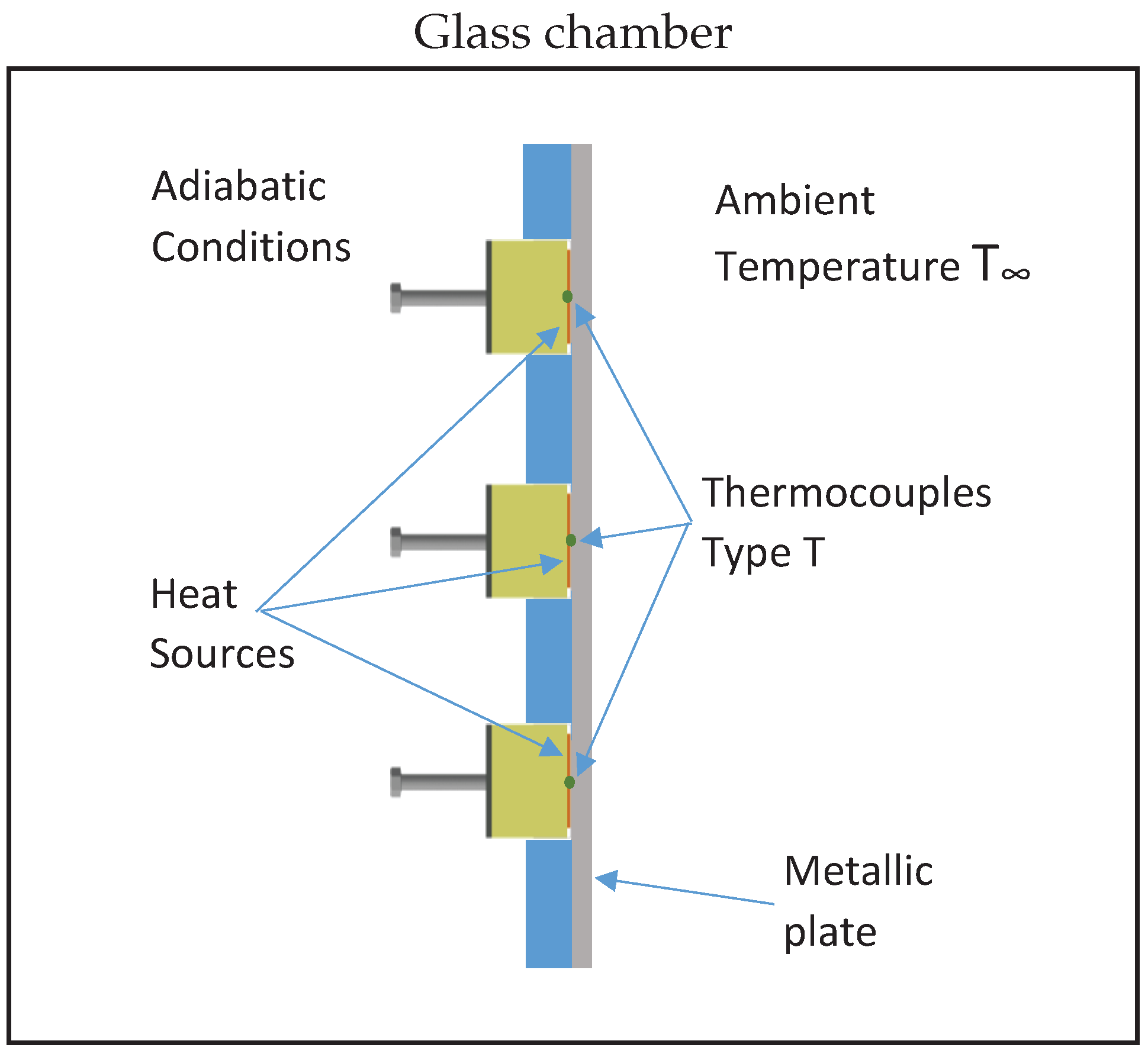
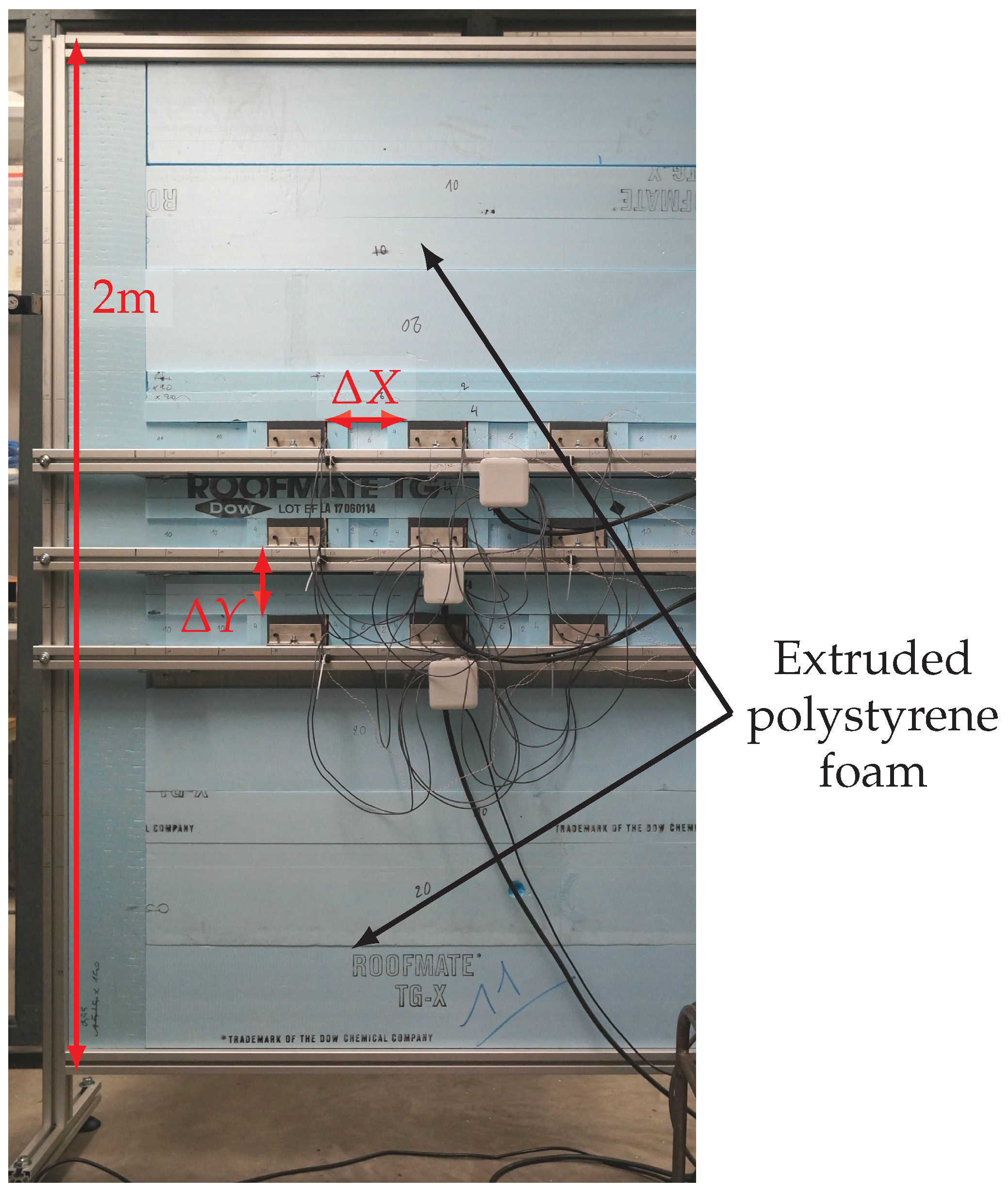
2.1. Experimental Setup
2.2. Measurements and Procedure
2.3. Optimal Distributions
3. Results
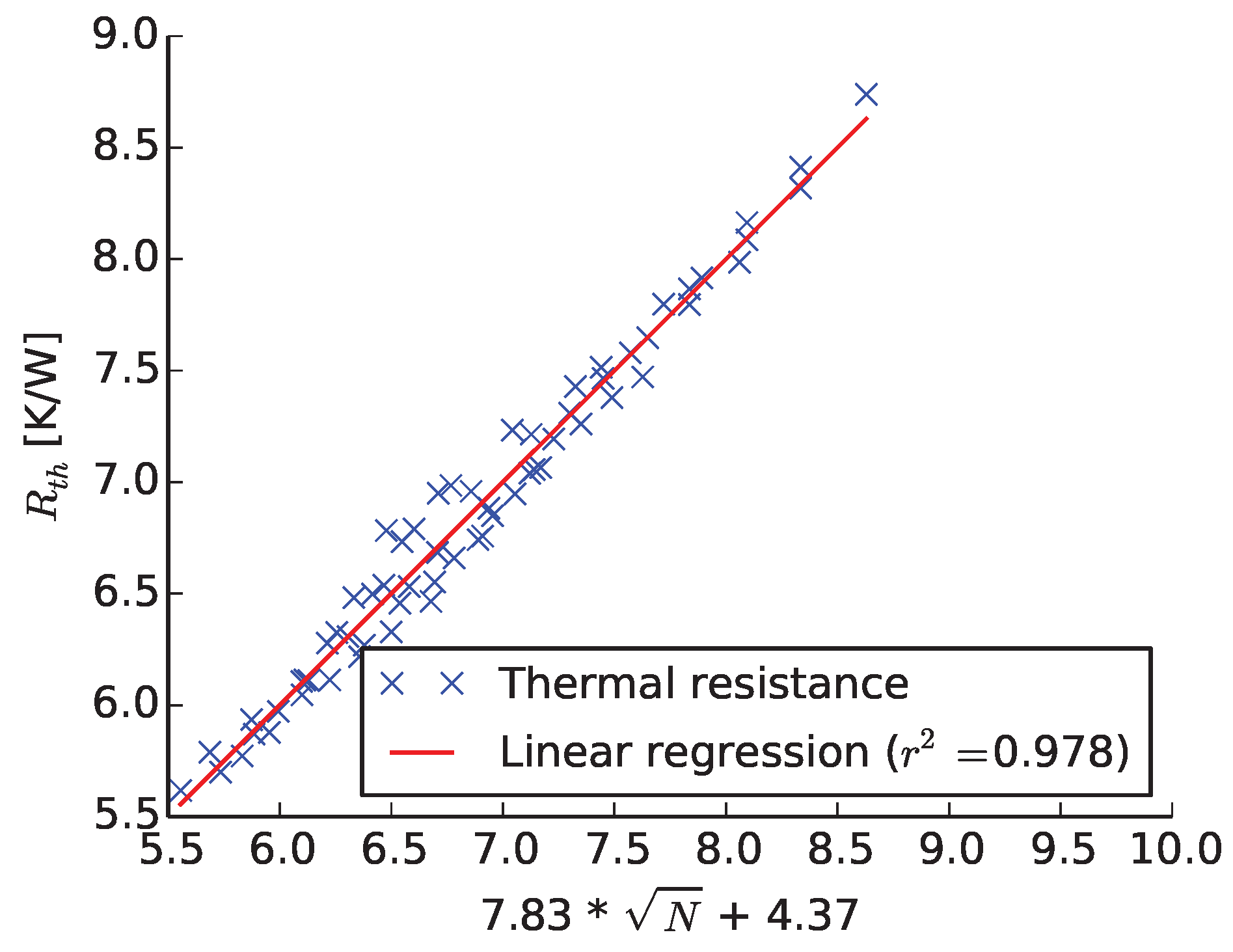
3.1. Measurements
3.2. Optima
4. Discussion
5. Conclusions
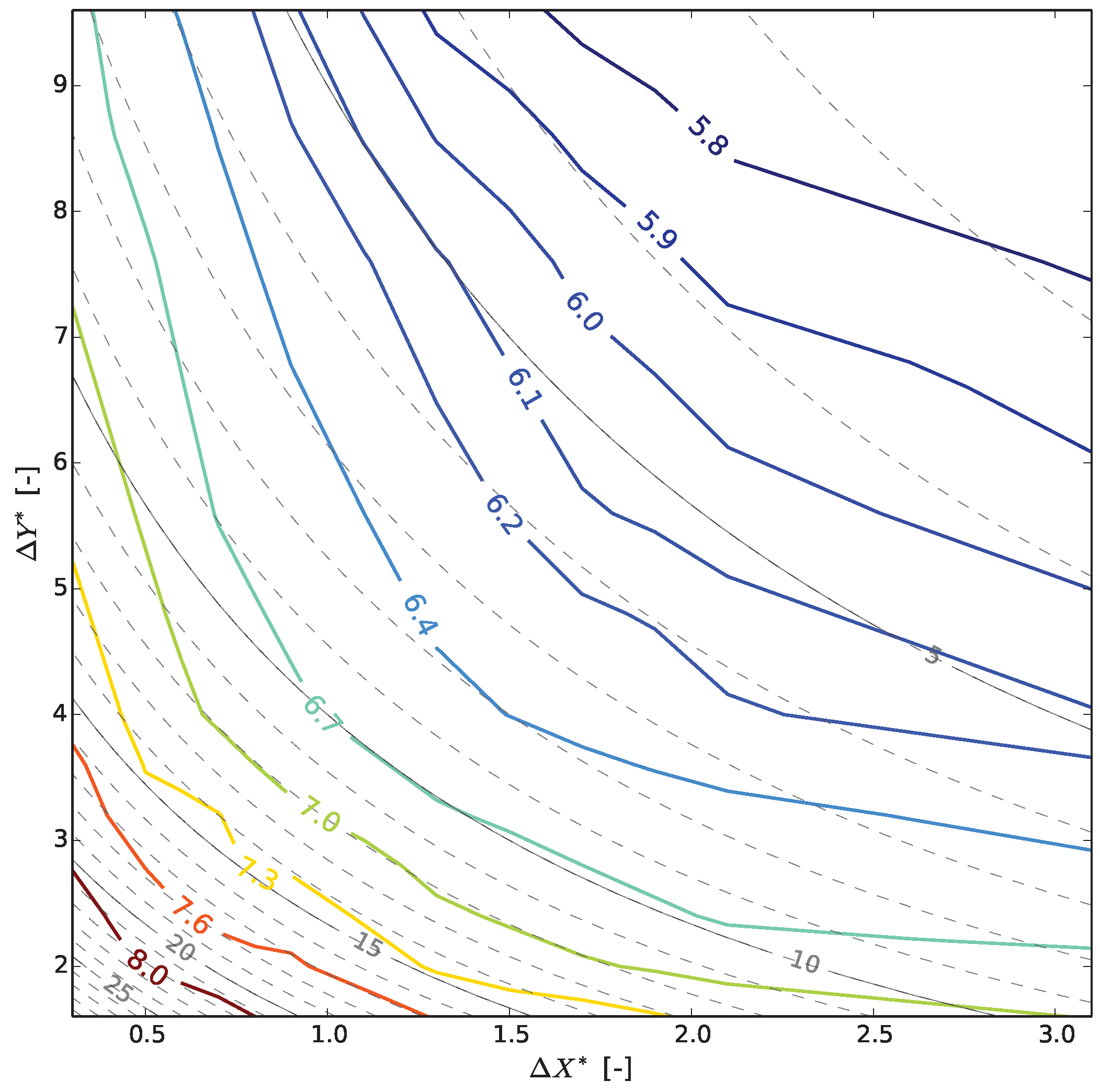
- the optimal vertical spacing varies faster than in the horizontal direction, due to convective thermal coupling;
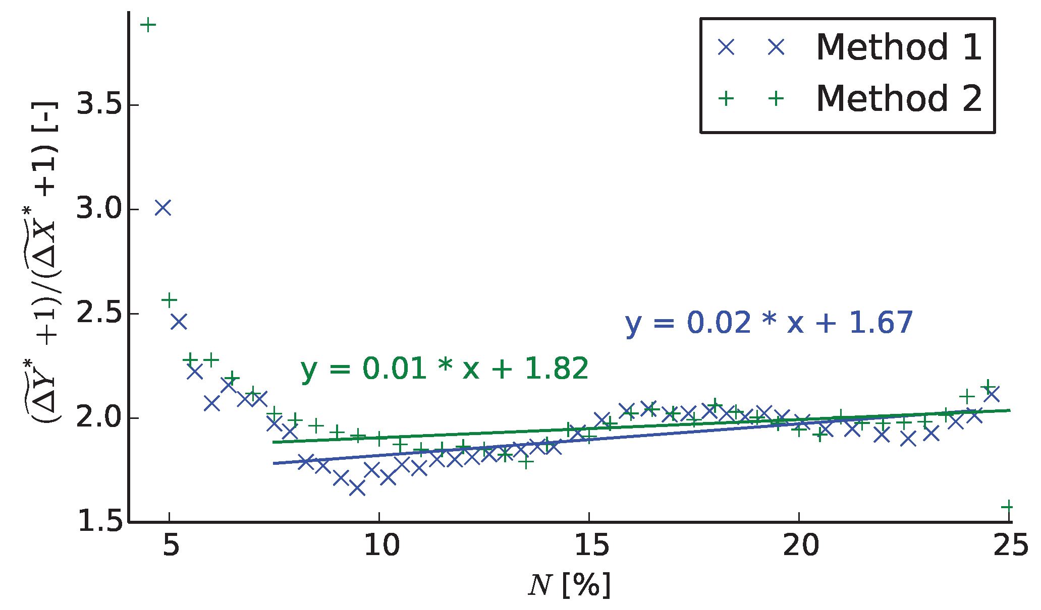
- the vertical spacing should be approximately twice as large as the horizontal spacing;
- the optimal ratio is almost independent of the heat source density;
- for higher densities, a slight increase was noticed for the optimal ratio as a function of the objective density.
Acknowledgments
Author Contributions
Conflicts of Interest
Abbreviations
| g | Gravitational constant | m/s2 |
| L | Heat source width | m |
| H | Heat source height | m |
| N | Heat source density | % |
| U | Voltage | V |
| I | Current | A |
| Thermal resistance | K/W | |
| α | Thermal diffusivity | m2/s |
| β | Volumetric thermal expansion coefficient | K−1 |
| Horizontal and vertical spacing | m | |
| Dimensionless horizontal spacing | - | |
| Dimensionless vertical spacing | - | |
| Optimal spacing | - | |
| Temperature excess () | K | |
| λ | Thermal conductivity | W/m.K |
| ν | Kinematic viscosity | m2/s |
References
- Barstow, S.F.; Haug, O.; Krogstad, H.E. Satellite altimeter data in wave energy studies. In Proceedings of the Third International Symposium Waves, Virginia Beach, VA, USA, 3–7 November 1997.
- Falnes, J. A review of wave-energy extraction. Mar. Struct. 2007, 20, 185–201. [Google Scholar] [CrossRef]
- Sjolte, J.; Tjensvoll, G.; Molinas, M. Power collection from wave energy farms. Appl. Sci. 2013, 3, 420–436. [Google Scholar] [CrossRef]
- Ekström, R.; Baudoin, A.; Rahm, M.; Leijon, M. Marine substation design for grid-connection of a research wave power plant on the swedish west coast. In Proceedings of the 10th European Wave and Tidal Conference (EWTEC), Aalborg, Denmark, 2–5 September 2013.
- Müller, N.; Kouro, S.; Glaria, J.; Malinowski, M. Medium-voltage power converter interface for wave dragon wave energy conversion system. In Proceedings of the IEEE Energy Conversion Congress and Exposition, Denver, CO, USA, 15–19 September 2013.
- Ma, K.; Liserre, M.; Blaabjerg, F.; Kerekes, T. Thermal loading and lifetime estimation for power device considering mission profiles in wind power converter. IEEE Trans. Power Electron. 2015, 30, 590–602. [Google Scholar] [CrossRef]
- Kovaltchouk, T.; Aubry, J.; Multon, B.; Ahmed, H.B. Influence of igbt current rating on the thermal cycling lifetime of a power electronic active rectifier in a direct wave energy converter. In Proceedings of the 2013 15th European Conference on Power Electronics and Applications (EPE), Lille, France, 2–6 September 2013.
- Sjolte, J.; Tjensvoll, G.; Molinas, M. Reliability analysis of igbt inverter for wave energy converter with focus on thermal cycling. In Proceedings of the 2014 Ninth International Conference on Ecological Vehicles and Renewable Energies (EVER), Monte-Carlo, Monaco, 25–27 March 2014.
- Baudoin, A.; Boström, C. Thermal modelling of a passively cooled inverter for wave power. IET Renew. Power Gener. 2015, 9, 389–395. [Google Scholar] [CrossRef]
- Faghri, A. Heat pipes: Review, opportunities and challenges. Front. Heat Pipes (FHP) 2014, 5. [Google Scholar] [CrossRef]
- Chowdhury, I.; Prasher, R.; Lofgreen, K.; Chrysler, G.; Narasimhan, S.; Mahajan, R.; Koester, D.; Alley, R.; Venkatasubramanian, R. On-chip cooling by superlattice-based thin-film thermoelectrics. Nat. Nanotechnol. 2009, 4, 235–238. [Google Scholar] [CrossRef] [PubMed]
- Gururatana, S. Heat transfer augmentation for electronic cooling. Am. J. Appl. Sci. 2012, 9, 436. [Google Scholar]
- Royne, A.; Dey, C.J.; Mills, D.R. Cooling of photovoltaic cells under concentrated illumination: A critical review. Solar Energy Mater. Solar Cells 2005, 86, 451–483. [Google Scholar] [CrossRef]
- Le Masson, S.; Nörtershäuser, D.; Mondieig, D.; Louahlia-Gualous, H. Towards passive cooling solutions for mobile access network. Ann. Telecommun. 2012, 67, 125–132. [Google Scholar] [CrossRef]
- Huaiyu, Y.; Koh, S.; van Zeijl, H.; Gielen, A.; Guoqi, Z. A review of passive thermal management of led module. J. Semicond. 2011, 32, 014008. [Google Scholar]
- Baïri, A.; Zarco-Pernia, E.; De María, J.-M.G. A review on natural convection in enclosures for engineering applications. The particular case of the parallelogrammic diode cavity. Appl. Therm. Eng. 2014, 63, 304–322. [Google Scholar] [CrossRef]
- Heindel, T.; Ramadhyani, S.; Incropera, F. Conjugate natural convection from an array of discrete heat sources: Part 1—two-and three-dimensional model validation. Int. J. Heat Fluid Flow 1995, 16, 501–510. [Google Scholar] [CrossRef]
- Tou, S.; Tso, C.; Zhang, X. 3-d numerical analysis of natural convective liquid cooling of a 3 × 3 heater array in rectangular enclosures. Int. J. Heat Mass Transf. 1999, 42, 3231–3244. [Google Scholar] [CrossRef]
- Sudhakar, T.; Balaji, C.; Venkateshan, S. A heuristic approach to optimal arrangement of multiple heat sources under conjugate natural convection. Int. J. Heat Mass Transf. 2010, 53, 431–444. [Google Scholar] [CrossRef]
- Hotta, T.K.; Venkateshan, S.P. Optimal distribution of discrete heat sources under natural convection using ann–ga based technique. Heat Transf. Eng. 2015, 36, 200–211. [Google Scholar] [CrossRef]
- Sudhakar, T.; Shori, A.; Balaji, C.; Venkateshan, S. Optimal heat distribution among discrete protruding heat sources in a vertical duct: A combined numerical and experimental study. J. Heat Transf. 2010, 132, 011401. [Google Scholar] [CrossRef]
- Habib, M.; Said, S.; Ayinde, T. Characteristics of natural convection heat transfer in an array of discrete heat sources. Exp. Heat Transf. 2014, 27, 91–111. [Google Scholar] [CrossRef]
- Sultan, G. Enhancing forced convection heat transfer from multiple protruding heat sources simulating electronic components in a horizontal channel by passive cooling. Microelectron. J. 2000, 31, 773–779. [Google Scholar] [CrossRef]
- Rajkumar, M.; Venugopal, G.; Lal, S.A. Natural convection from free standing tandem planar heat sources in a vertical channel. Appl. Therm. Eng. 2013, 50, 1386–1395. [Google Scholar] [CrossRef]
- Andreozzi, A.; Manca, O. Radiation effects on natural convection in a vertical channel with an auxiliary plate. Int. J. Therm. Sci. 2015, 97, 41–55. [Google Scholar] [CrossRef]
- Hajmohammadi, M.; Nourazar, S.; Campo, A.; Poozesh, S. Optimal discrete distribution of heat flux elements for in-tube laminar forced convection. Int. J. Heat Fluid Flow 2013, 40, 89–96. [Google Scholar] [CrossRef]
- Öztop, H.F.; Estellé, P.; Yan, W.-M.; Al-Salem, K.; Orfi, J.; Mahian, O. A brief review of natural convection in enclosures under localized heating with and without nanofluids. Int. Commun. Heat Mass Transf. 2015, 60, 37–44. [Google Scholar] [CrossRef]
- Narasimham, G. Natural convection from discrete heat sources in enclosures: An overview. Vivechan Int. J. Res. 2010, 1, 63–78. [Google Scholar]
- Da Silva, A.; Lorente, S.; Bejan, A. Optimal distribution of discrete heat sources on a wall with natural convection. Int. J. Heat Mass Transf. 2004, 47, 203–214. [Google Scholar] [CrossRef]


| Parameter | Value |
|---|---|
| Metal plate | 200 × 150 cm |
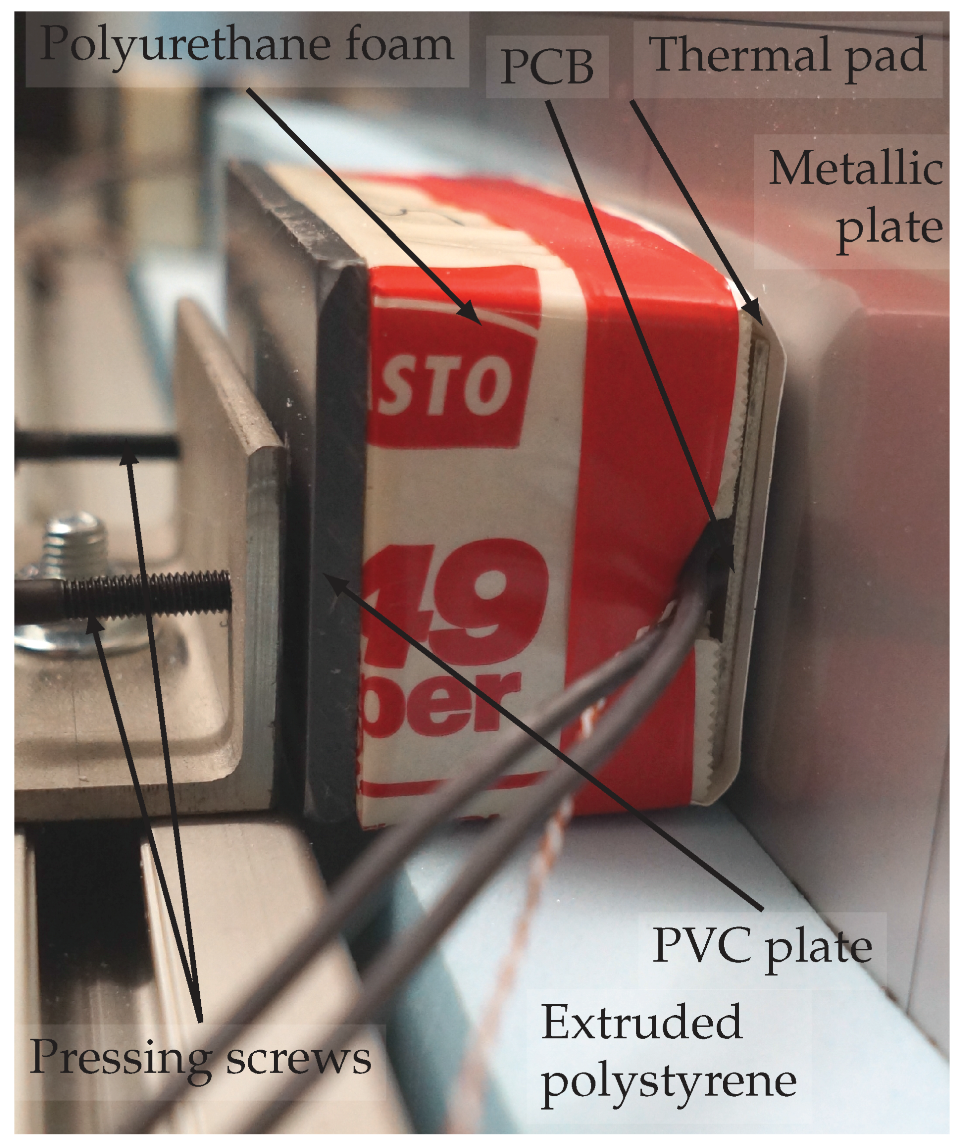
| PCB heating plates (thickness) | 5 × 10 cm (1.6 mm) |
| Thermal sheet thickness | 0.2 mm |
| Polyurethane foam (thickness) | 6 × 11 cm (40 mm) |
| PVC plate (thickness) | 6 × 11 cm (5 mm) |
| Extruded polystyrene thickness | 30–40 mm |
| ΔX | 3, 5, 7, 9, 13, 17, 21, 31 |
| ΔY | 8, 10, 12, 16, 20, 28, 38, 48 |
© 2016 by the authors; licensee MDPI, Basel, Switzerland. This article is an open access article distributed under the terms and conditions of the Creative Commons Attribution (CC-BY) license (http://creativecommons.org/licenses/by/4.0/).
Share and Cite
Baudoin, A.; Saury, D.; Zhu, B.; Boström, C. Experimental Optimization of Passive Cooling of a Heat Source Array Flush-Mounted on a Vertical Plate. Energies 2016, 9, 912. https://doi.org/10.3390/en9110912
Baudoin A, Saury D, Zhu B, Boström C. Experimental Optimization of Passive Cooling of a Heat Source Array Flush-Mounted on a Vertical Plate. Energies. 2016; 9(11):912. https://doi.org/10.3390/en9110912
Chicago/Turabian StyleBaudoin, Antoine, Didier Saury, Bo Zhu, and Cecilia Boström. 2016. "Experimental Optimization of Passive Cooling of a Heat Source Array Flush-Mounted on a Vertical Plate" Energies 9, no. 11: 912. https://doi.org/10.3390/en9110912