Optimal Hierarchical Control for Smart Grid Inverters Using Stability Margin Evaluating Transient Voltage for Photovoltaic System

Abstract

This research proposed an optimal control approach for a smart grid electrical system with photovoltaic generation, where the control variables are voltage and frequency, which aims to improve the performance through addressing the need for a balance between the minimization of error and the operational cost. The proposed control scheme incorporates the latest advancements in heuristics and hierarchical control strategies to provide an efficient and effective solution for the smart grid electrical system control. Implementing the optimal control scheme in a smart power grid is expected to bring significant benefits, such as the reduced impact of renewable energy sources, improved stability, reliability and efficiency of the power grid, and enhanced overall performance. The optimal coefficient values are found by minimizing the cost functions, which leads to a more efficient system performance. The voltage output response of the system in a steady state is over-damped, with no overshoot, but with a 5% oscillation around the target voltage level that remains consistent. Despite the complexity of nonlinear elements’ behavior and multiple system interactions, the response time is fast and the settling time is less than 0.4 s. This means that even with an increase in load, the system output still meets the power and voltage requirements of the system, ensuring efficient and effective performance of the smart grid electrical systems.

1. Introduction

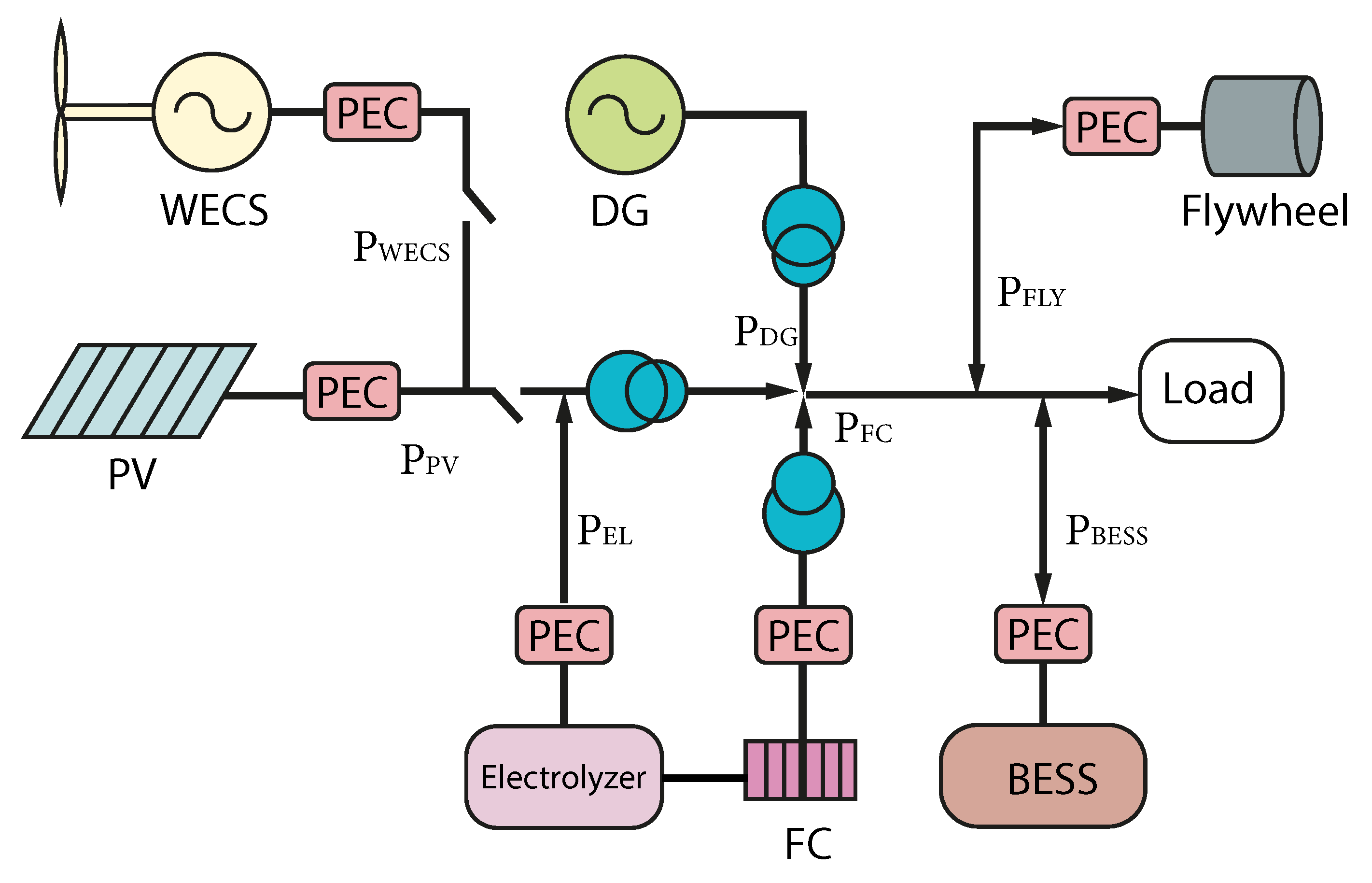
A microgrid (MG) system operates primarily in alternating current (AC), but it also includes several direct current (DC) loads, such as energy storage systems (ESS) and new technological loads [1]. There are various MG configurations available, each with its own unique features, advantages, and drawbacks, depending on the specific application. For instance, some configurations are designed to prioritize reliability and resilience, while others prioritize efficiency and cost-effectiveness. Choosing the right configuration is critical to ensuring that the MG system meets the needs of its users and operates effectively. Researchers have been exploring different configurations and evaluating their performance to identify the best option for specific applications [2]. As the demand for MG systems continues to grow, it is crucial to continue this research and development work to ensure that MG systems continue to meet the needs of their users and deliver the desired outcomes. Thus, a hybrid AC/DC MG combines DC and AC devices, joining the best of both worlds characteristics [3]. The hybrid MG, on the one hand, integrates new renewable energy resources (RES), has high reliability, and a low maintenance cost [4]. On the other hand, hybrid MG has high dimensions, low scalability capacity, and a medium capacity for controllability and fault management. As a result, the MG challenges future research topics, for example, control strategies, efficiency, and reliability improvement [5,6]. The hybrid MG depicted in Figure 1 encompasses various DC generators, such as photovoltaic (PV), electrolyte, fuel cells (FC), and diesel generator, all of which work together to regulate system frequency. Additionally, the system includes two energy storage components, a flywheel and a battery-based Energy Storage System (BESS). The Power Energy Converter (PEC) is responsible for linking the load to the system and its different elements in an efficient manner [7,8].

This proposed optimal control minimizes the error for loop control, but maintains an acceptable operational cost. The system implements a controller, which implements an optimal hierarchical control system (HCS). It minimizes the absolute error and improves power quality, considering frequency and voltage parameters [9,10]. The MG controller implemented achieves superior performance compared to other available systems, as it effectively regulates voltage, frequency, and power, facilitates load sharing, coordinates RES, and synchronizes with the primary grid. Additionally, it optimizes the operating cost as reported in [11]. The proposed control structures have been designed to enhance the stability of the transition during different disturbances, as reported in [12,13]. Furthermore, it is believed that the control can be optimized using algorithms to address the control problem and minimize the absolute error in steady-state, as highlighted in [10]. These algorithms are expected to provide improved performance and greater accuracy in controlling the system, leading to a more stable and efficient operation. By integrating these control structures and algorithms into the system, the goal is to achieve a robust and reliable MG that can effectively handle different disturbances and provide stable and consistent power to its users. Overall, the proposed control structures and algorithms represent a significant advancement in the field of MG control and have the potential to benefit many different applications.

The research proposes the control strategy into primary and secondary control. The primary control keeps the electrical parameters in a specific range, while the secondary control guarantees the economic and reliable system operation [10,14]. This research explores the optimization techniques for optimal control; an objective function can minimize the energy consumption or the response time; also, it can maximize the system reliability, and controller robustness [15].

The paper demonstrates the validity of its strategy by comparing the results to those of similar techniques based on parameters such as computational cost and transient response. Additionally, a system performance analysis is presented, evaluating the response to various types of faults, including incipient, instantaneous, and abrupt changes, as well as the total harmonic distortion (THD) percentage [16].

There is some research in the field. In [17,18] a detailed MG description is presented, including the main system features and the classical control strategies. The paper [19] compares MG implemented in different geographical regions and defines their features, including the existing MG test-beds. Ref. [20] reviewed the major issues and challenges in MG control; also, the authors classified the control into three levels, primary, secondary and tertiary. Therefore, ref. [21] proposed an autonomous droop scheme for energy MG management in grid or stand-alone modes. Finally, ref. [22,23] designed a power management system for a hybrid MG.

The document is structured in a clear and concise manner, with Section 2 showcasing the methodology used, Section 3 presenting the results and analysis, and Section 4 summarizing the conclusions and outlining potential future work. The document provides a comprehensive overview of the study, presenting the key findings and their implications in a clear and straightforward manner.

2. Methodology

The MG has several outputs, including voltage and current work, which must follow particular behavior. The controller is responsible for that behavior, and those output signal oscillations are damped in a transient state. The controller analysis evaluates those oscillations in the transition of operation modes [10].

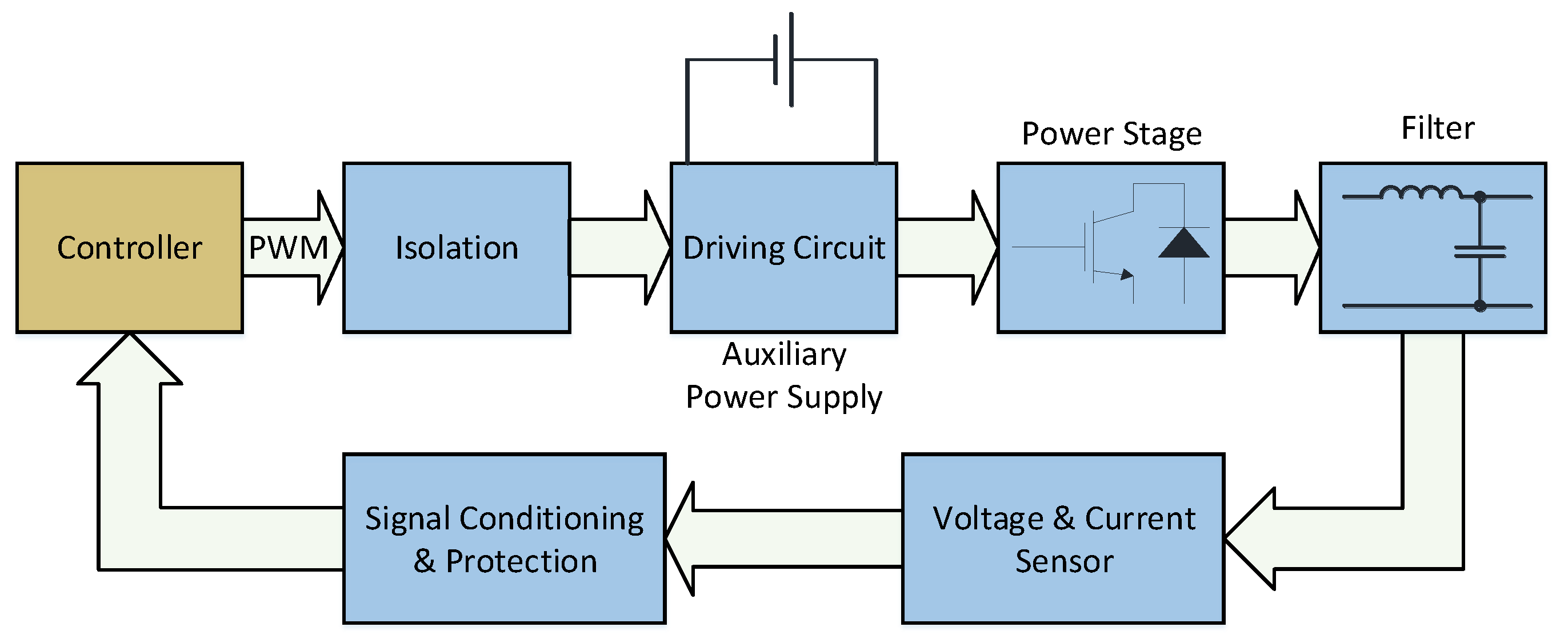
A HCS typically reduces the parameters of MG external variations and links the external loops actions [24]. Therefore, HCS coordinates the entire controller actions, beginning in the primary control and reaching the higher available level in a MG system [25]. The hierarchical strategy starts with primary control, the lower level, which implements the voltage and current control loops. Figure 2 shows a schematic diagram of the system’s primary control and electrical elements, starting from the power stage, which implements the PEC.

The primary level can be designed through different strategies; for instance, impedance control. The primary control reference signal is calculated employing the secondary control system [26,27].

Table 1. Parameters and variables for primary control.

Nomenclature	Description
$K_p$	Proportional gain for controller
$K_i$	Integral term for controller
$K_d$	Derivative term for controller
$K_{cr}$	Critical gain for oscillation
$P_{cr}$	Oscillation period in resonance
${\omega }_{cg}$	Oscillation frequency in resonance
$T_{ii}$	Integral time term for current loop
$T_{di}$	Derivative time term for current loop
GM	Gain Margin
N	Gain for the derivative filter
$DE{N}_{PI}$	Denominator PI controller
$DE{N}_{PID}$	Denominator PID controller
$G_C$	Transfer function for controller
$G_v$	Voltage controller transfer function
$K_{pv}$	Proportional gain for controller
$K_{rv}$	Resonant term for controller
${\omega }_c$	Resonant frequency
${\omega }_0$	Fundamental frequency

shows the system parameters. The control approach adopts a cascade structure, utilizing an inner loop for current control and an outer loop for voltage control. This structure brings several benefits, such as reducing the THD in the voltage filter capacitor, ensuring the inductor filter current stays within operational limits, effectively rejecting disturbances, and enabling a change in the active mode while preserving the control scheme [28].

Multiple strategies exist for designing the current and voltage control loops. In this research, the inner loop is designated as the primary control as it plays a critical role in ensuring the maximum power point (MPP) is reached. In grid-connected systems, MPP tracking requires a specific current and voltage to be maintained. In stand-alone systems, the energy produced depends on the load demands [29].

In Figure 3, the control scheme for primary control is shown. The $\alpha$ and $\beta$ sequences used stationary reference frames through the Clarke transformation, which are expressed by Equation (1). This transformation changes the 3-phase frame to the $\alpha \beta$ and zeroes input to simplify the calculation due to its stationary behavior [30].

$$\left[\begin{array}{c}\alpha \\ \beta \\ 0\end{array}\right]=\frac{2}{3}\left[\begin{array}{ccc}1& -\frac{1}{2}& -\frac{1}{2}\\ 0& \frac{\sqrt{3}}{2}& -\frac{\sqrt{3}}{2}\\ \frac{1}{2}& \frac{1}{2}& \frac{1}{2}\end{array}\right]\left[\begin{array}{c}a\\ b\\ c\end{array}\right]$$

(1)

The applied method represents the voltage feedback, which regulates the voltage by comparing the output voltage with its reference value [31]. The same for the primary current loop, which compares the output inductor current with the reference voltage received from the voltage loop.

Figure 3 shows the primary control, including the blocks representing the defined plant. Before the $G_{PWM}$ block, there is the current controller $G_I$, using the PID controller, implemented to follow the reference current. The feedback loop includes the relation $1/Z_C$, which transforms the output voltage into current to subtract it from the reference current, $I{l}_{ref}$. Before it, there is the voltage controller $G_V$, applying the Proportional Resonant (PR) scheme to follow the reference voltage received from the secondary control and subtract the feedback output voltage [32,33].

The current and voltage control strategy is essential in the final performance system [34]. The current loop injects a high gain into the frequency reference signal, thus increasing the disturbance system rejection, as shown by Equation (2). However, the voltage control strategy reduces the THD if there are nonlinear loads in the system, see Equation (3). The voltage controller is responsible for controlling the capacitor filter voltage and comparing it with the reference signal received from the secondary loop. However, the output of the voltage loop serves as the reference current for the inner current loop. The inner loop dynamics should be faster than the outer loop; this strategy maintains the stability in the system [35,36]. The PID tuning controller strategy, known as the generalized forced oscillation method, is implemented in the PID controller of Equation (2). The PID controller includes a first-order system and a low-pass filter to minimize the effect of noise in the control variables. This strategy is widely used due to its ease of implementation, flexibility and effectiveness in controlling various processes. The PID controller is one of the most commonly used structures in the industry and has proven to be an effective tool for controlling dynamic systems. PID tuning is calculated with Ziegler and Nichols (ZN) [37], using the Algorithms 1 and 2 [37,38].

$$G_i\left(s\right)=K_{pi}\left(1+\frac{1}{T_{ii}s}+\frac{T_{di}s}{\frac{T_{di}}{N}s+1}\right)$$

(2)

An integral action can solely control all the systems; the constraint is that the system must have a minimum phase. However, the controller can cause a poor transient response. A proposed solution is adding a proportional element to achieve closed-loop stability and robustness [39].

The inner loop control can be used for any ZN tuning process, where defining the transfer function for the controlled plant is essential. After that, a PR is connected in series. Here, two methods are used if the gain margin is determined through mathematical tools and can be used directly. While the other possibility is applying the increase of the proportional gain towards the plant oscillation method in a closed-loop [40].

The frequency where the gain margin is located in the $W_{cg}$ is part of the tuning process. Different methodologies, such as PR, can be implemented if the gain margin is not computed. Algorithm 2 calculates the PID coefficients using the result from Algorithm 1. In step 2, the pole’s controller is determined. It depends on the selected controller, are 2 or 3, depending on whether a PI or PID is desired. Additionally, the PI or PID variables can be expressed as the time constant to be implemented in some industrial devices. Finally, the controller denominator is an integrator s.

The PR controller was chosen for the voltage loop, as it has an infinite gain margin, making it difficult to find a PID controller with Ziegler–Nichols (ZN) tuning. The implementation of the PR controller improves the voltage performance by reducing harmonics and minimizing steady-state errors, as expressed in Equation (3) [41]. This ultimately leads to a more stable and efficient performance in the system.

$$G_v\left(s\right)=k_{pv}+\frac{k_{rv}s}{s^2+{\omega }_{c}s+{\omega }_0^2}$$

(3)

The PR controller has a resonant frequency that aligns with the reference signal, allowing it to follow a sinusoidal reference signal effectively. Pure integral control is a particular type of PR controller, and compared with PID classical controllers, it is seen that the computation cost increases. The PID modifies the phase and amplitude of the signal components, thus causing a delay in the control loop, and this solution can affect the overall performance [33,39].

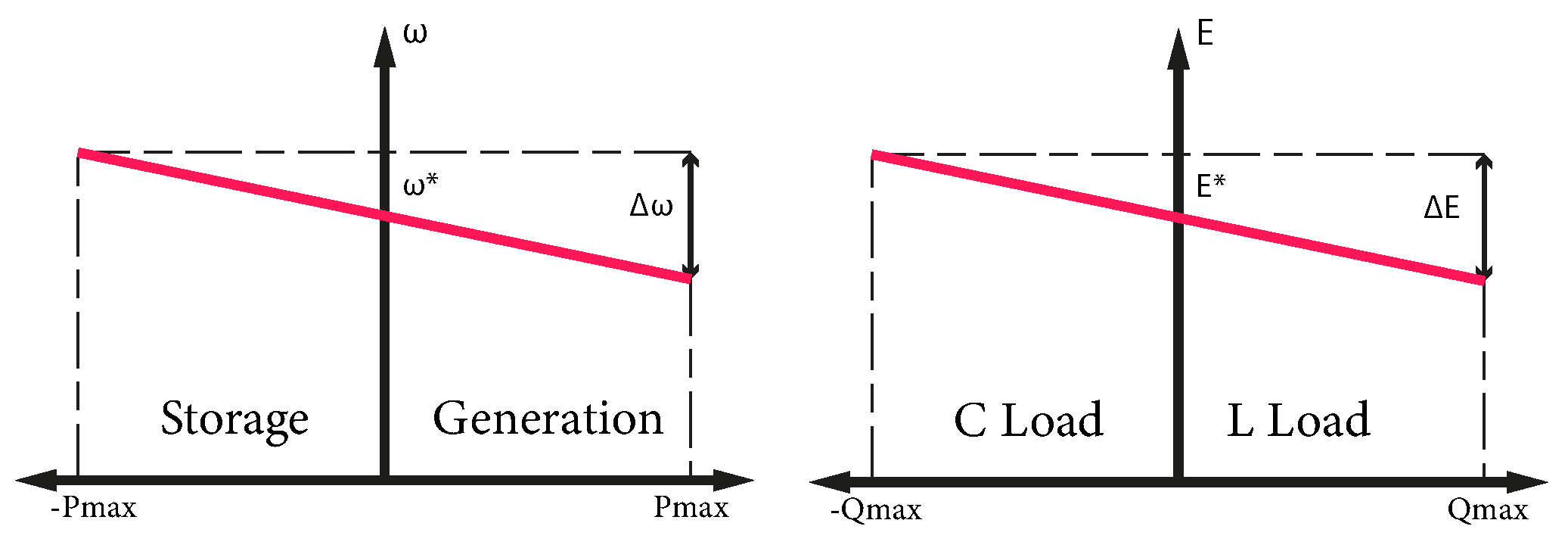
In a microgrid, several voltage source inverters (VSI) are connected in parallel to produce a net interchange. The secondary control sets the reference frequency and voltage for the inner loop while implementing power sharing through P-f and Q-V droop control (as shown in Figure 4). The compensation, represented by m and n or deviations of $\delta Q/\delta V$ and $\delta P/\delta \omega$, helps to maintain synchronization within the voltage and stability limits of the system.

Algorithm 1 Tuning procedure for open loop system using ZN.

1:  procedure ZN tuning($K_{cr},P_{cr}$) 2:     Step: 1 Variables definition 3:     $K_p,K_i,K_d,K_{cr},P_{cr}$ 4:     Step: 2 Plant Definition 5:     Determining the complete transfer function 6:     $G_1\leftarrow \frac{\frac{Z_C}{Z_L}}{1+\frac{Z_C}{Z_L}}$ 7:     $G_P\leftarrow G_{PWM}\ast G_1$ 8:     Step: 3 Eliminating components controller 9:     Guaranteeing proportional controller 10:     $K_i\leftarrow 0$ 11:     $K_d\leftarrow 0$ 12:     Step: 4 Proportional controller 13:     K proportional constant 14:     $G\leftarrow K\ast G_P$ 15:     Step: 5 Determine gain margin 16:     if GM is determined = $True$ then 17:         $K_{cr}=GM$ 18:     else 19:         while $K=O:constant:K_{cr}$ do 20:            if Closed loop GP is oscillating then 21:                $K_{cr}=K$ 22:         if GM = ∞ then 23:            Applied PR controller 24:     Step: 6 Oscillation period 25:     $W_{cg}$ where GM is measured 26:     $P_{cr}\leftarrow \frac{2\pi }{W_{cg}}$                ▹ Ending

Algorithm 2 PID initial coefficient using ZN tuning.

1: procedurePID initial($G_c$) 2:     Step: 1 Variables definition 3:     $K_p,K_i,K_d,T_i,T_d,K_{cr},P_{cr}$ 4:     Step: 2 PID denominator 5:     if $case=1$ then 6:         PI controller 7:         $De{n}_{PI}=\frac{K_{cr}}{2.2}\left[\begin{array}{cc}1& \frac{1.2}{P_{cr}}\end{array}\right]$ 8:     if $case=2$ then 9:         PID controller 10:         $De{n}_{PID}=\frac{2\ast K_{cr}}{1.7\ast P_{cr}}\left[\begin{array}{ccc}\frac{P_{cr}}{8}& 1& \frac{2}{P_{cr}}\end{array}\right]$ 11:     Step: 3 Defining independent constants 12:     $K_p\leftarrow De{n}_{PI}\left(1\right)$ 13:     $T_i\leftarrow De{n}_{PI}\left(2\right)$ 14:     if $De{n}_{PD}\left(2\right)\ne 0$ then 15:         $T_d\leftarrow De{n}_{PI}\left(3\right)$ 16:     $K_i\leftarrow \frac{K_p}{T_i}$ 17:     $K_d\leftarrow K_p{T}_d$ 18:     Step: 4 Proportional controller 19:     K proportional constant 20:     $G\leftarrow K\ast G_P$ 21:     Step: 5 Defining controller 22:     if $case=1$ then 23:         PD controller 24:         $G_c\leftarrow \frac{De{n}_{PI}}{s}$ 25:     if $case=2$ then 26:         PID controller 27:         $G_c\leftarrow \frac{De{n}_{PID}}{s}$

▹ Ending

The equations that describe the droop control are presented in Equations (4) and (5). $\omega$ and E denote the frequency and voltage, respectively, while $\omega$* and E* are the respective references for these quantities. $G_P\left(s\right)$ and $G_Q\left(s\right)$ are the control transfer functions, which cannot be implemented by pure integral control, particularly in the islanded mode, due to the mismatch between the total injected power and the total power [42]. The system parameters are shown in

Table 2. Parameters and variables for secondary and tertiary control.

Nomenclature	Description
$G_P$	Transfer function for active power controller
$G_Q$	Transfer function for reactive power controller
$G_F$	Filter transfer function
${\delta }_E$	Voltage variation
${\delta }_{\omega }$	Frequency variation
$K_e$	Proportional gain for controller
$V_{pcc}$	Point of common coupling voltage
n, $n_d$	Drop coefficients for P power control
m, $m_d$	Drop coefficients for Q power control
$k_{pE}$	Proportional gain for voltage deviation
$k_{iE}$	Integral gain for voltage deviation
$k_{p\omega }$	Proportional gain for frequency deviation
$k_{i\omega }$	Integral gain for frequency deviation
$G_{VR}$	Voltage restoration controller
$G_{FR}$	Frequency restoration controller
$G_{LPF}$	Filter transfer function
$G_d$	Primary order transfer function

.

$$\omega ={\omega }^{*}-G_P\left(s\right)(P-P^{*})$$

(4)

$$E=E^{*}-G_Q\left(s\right)(Q-Q^{*})$$

(5)

$$\dot{E}=\left[K_e(E^{*}+\delta E-V_{pcc})-n(P-P^{*})-G_F\ast n_d(P-P^{*})\right]$$

(6)

$$\omega =\left[{\omega }^{*}+\delta \omega +m(Q-Q^{*})+G_F\ast m_d(Q-Q^{*})\right]$$

(7)

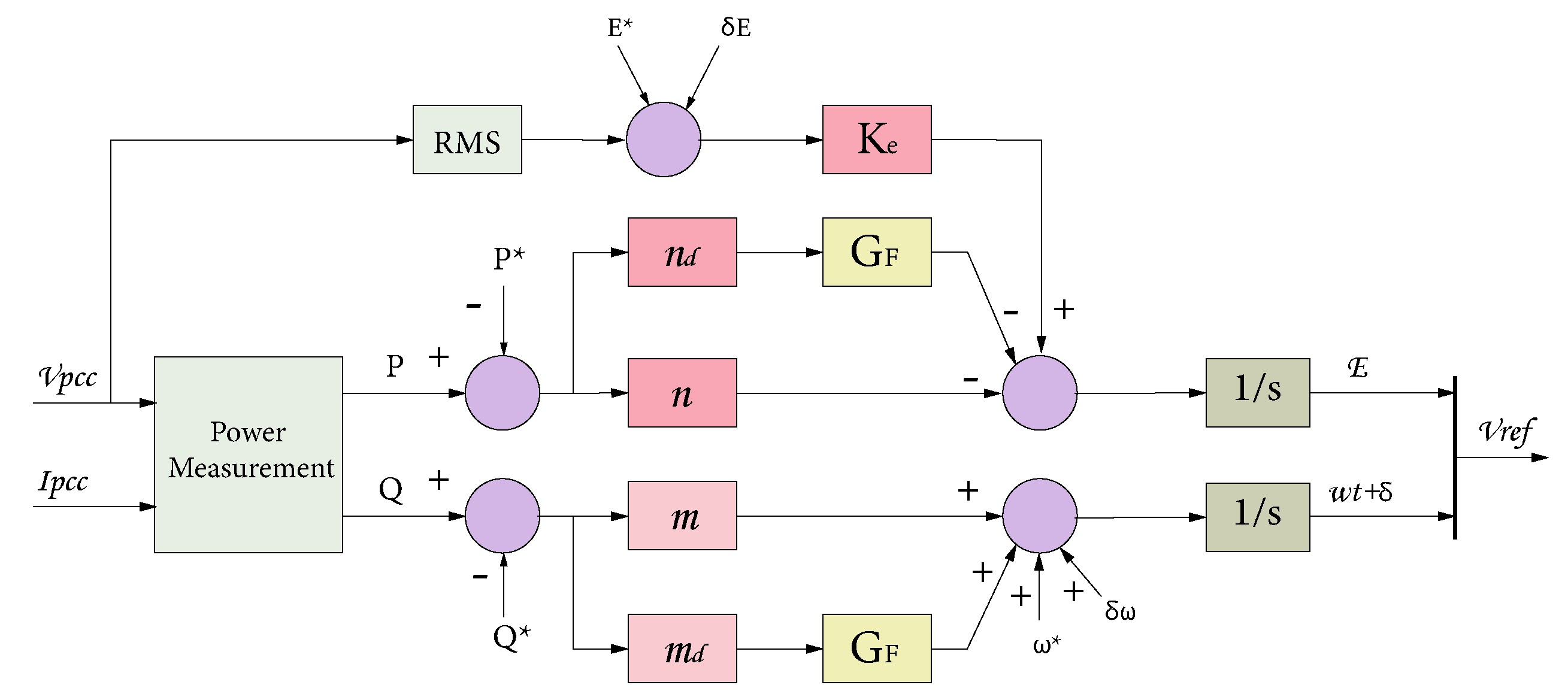
The control transfer functions $G_P\left(s\right)$ and $G_Q\left(s\right)$ are implemented using different control techniques in this research. The implementation uses the Universal Droop Control introduced by [43] as depicted in Equations (6) and (7) and illustrated in Figure 5. The RMS voltage (E) and frequency ($\omega$) are measured at the Point of Common Coupling (PCC), while the desired values for these magnitudes, E* and $\omega$, are set as the nominal values. The desired active and reactive power values, P and Q*, depend on whether the Microgrid (MG) is connected to the grid. In islanded mode, the desired values for active and reactive power are normally set to zero.

The droop control coefficients are denoted by “n” and “m” in the equations. They represent the deviation of the reactive power with respect to the voltage and the deviation of the active power with respect to the frequency, respectively. In addition, the coefficients related to the active and reactive power are represented by $n_d$ and $m_d$, respectively. To regulate the voltage at the PCC, a proportional controller constant $K_e$ is used. Moreover, to reduce the noise in the signal, a filter $G_f$ is implemented, which is described by Equation (10). Finally, the sample time for the current and voltage loop is in the order of milliseconds, while the sample time for the power control is in the order of seconds.

$$n=\frac{\Delta \omega }{P_{max}}$$

(8)

$$m=\frac{\Delta V}{2\ast Q_{max}}$$

(9)

$$G_F=\frac{100s}{100+s}$$

(10)

3. Results and Discussion

The primary control is implemented in the system with the parameters of

Table 3. Parameters for primary control.

Parameter	Symbol	Value
Gain margin	$GM$	2.15
Oscillation period	$P_{cr}$	0.116 m
Integral time term	$K_{pi}$	0.22
Derivative time term	$K_{ii}$	201.6
Proportional gain	$K_{pv}$	0.1
Resonant term	$K_{rv}$	209.9
Resonant frequency	${\omega }_c$	0.001 Hz
Filter gain	N	100

. The initial values for the optimization algorithm are the first and second parameters, $GM$ and $P_{cr}$, which are calculated as the gain margin and oscillation period, while the following parameters, $K_{pi}$, $K_{ii}$, $K_{pv}$, $K_{rv}$ and ${\omega }_c$, are the constants for the primary controller.

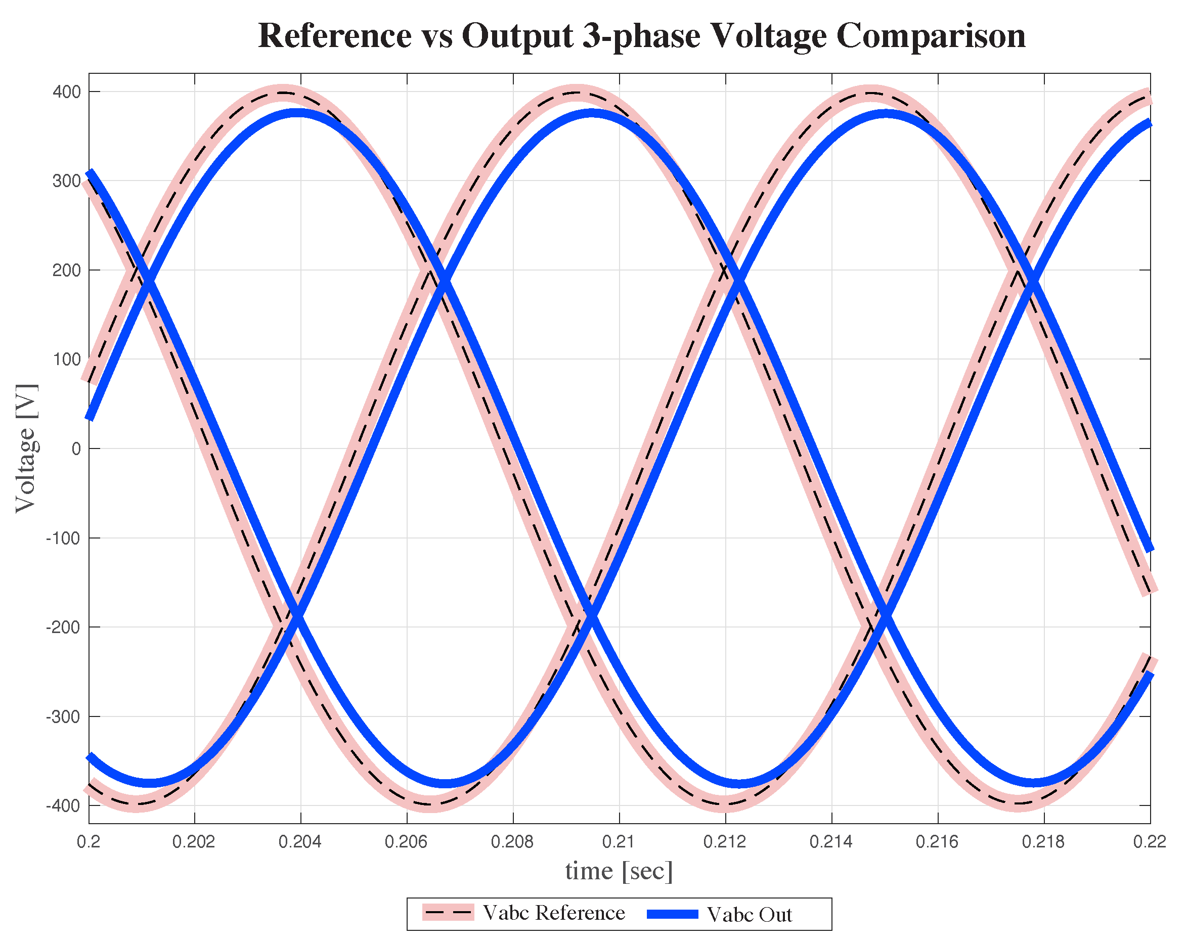
The system consists of a voltage and current controller, which are implemented using a PR and PID controller, respectively. The parameters were determined using the optimization algorithm proposed in the paper. The comparison between the system output and the reference voltage is shown in Figure 6, where the secondary controller calculates the system output, which serves as the input for the primary loop control. The reference voltage has an amplitude of 600 Vp and a frequency of 60 Hz, which are nominal values for MG.

The primary controller effectively tracks the reference signal, as shown by the graph. There is no delay between the signals, but there is a slight reduction in the maximum voltage. It presents a steady-state error in the system, which can be neglected because it is less than $5\%$.

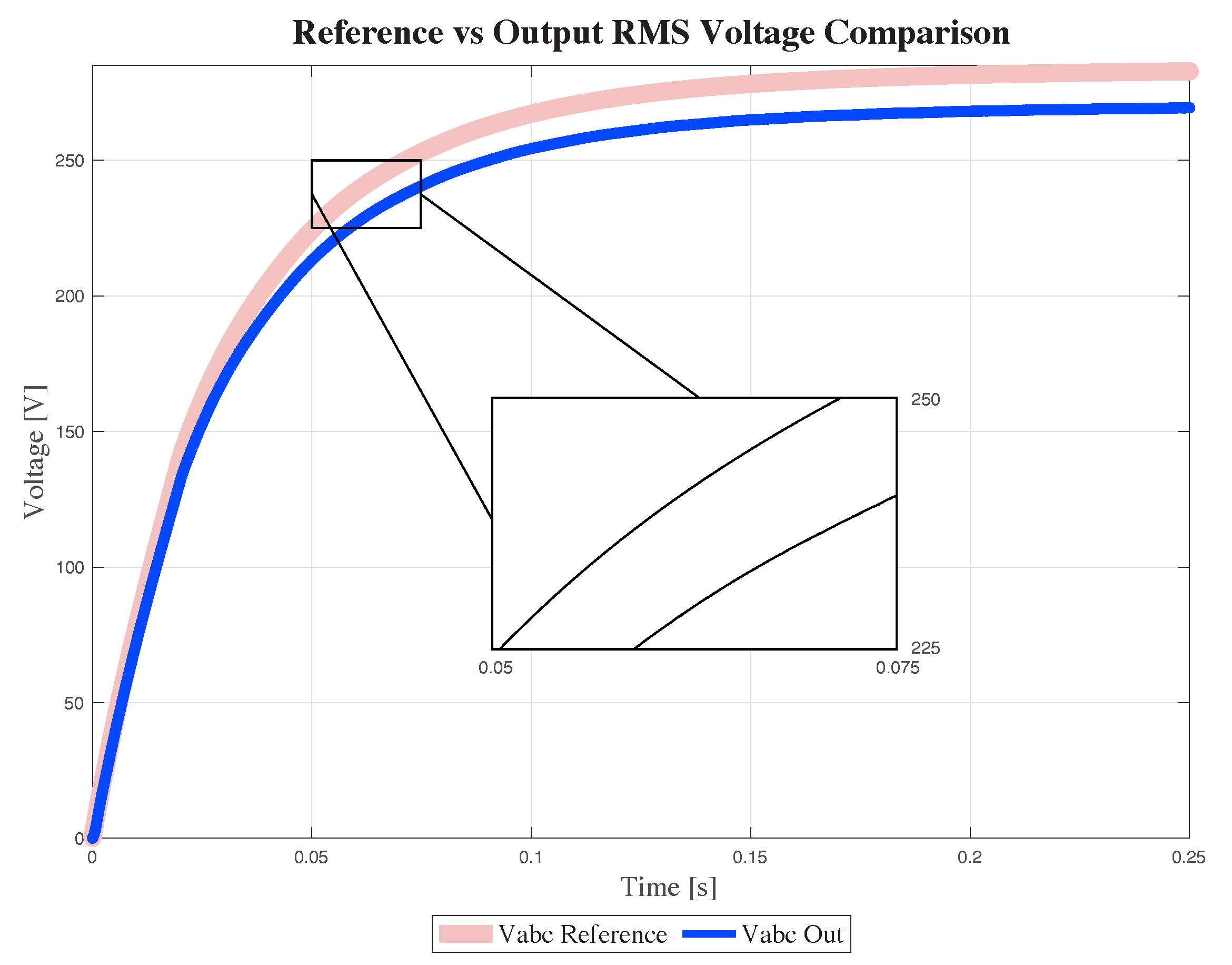
Additionally, the system stability is further confirmed by the RMS output results in Figure 7. The rise time to reach the nominal value of 600 Vp is quick, around 0.15 s, and the system exhibits an over-damped behavior with no overshoot. Although there are small fluctuations, roughly 5%, around the desired voltage, the pattern is consistent and the response is fast, indicating an acceptable performance given the complexity of the system and its multiple interactions.

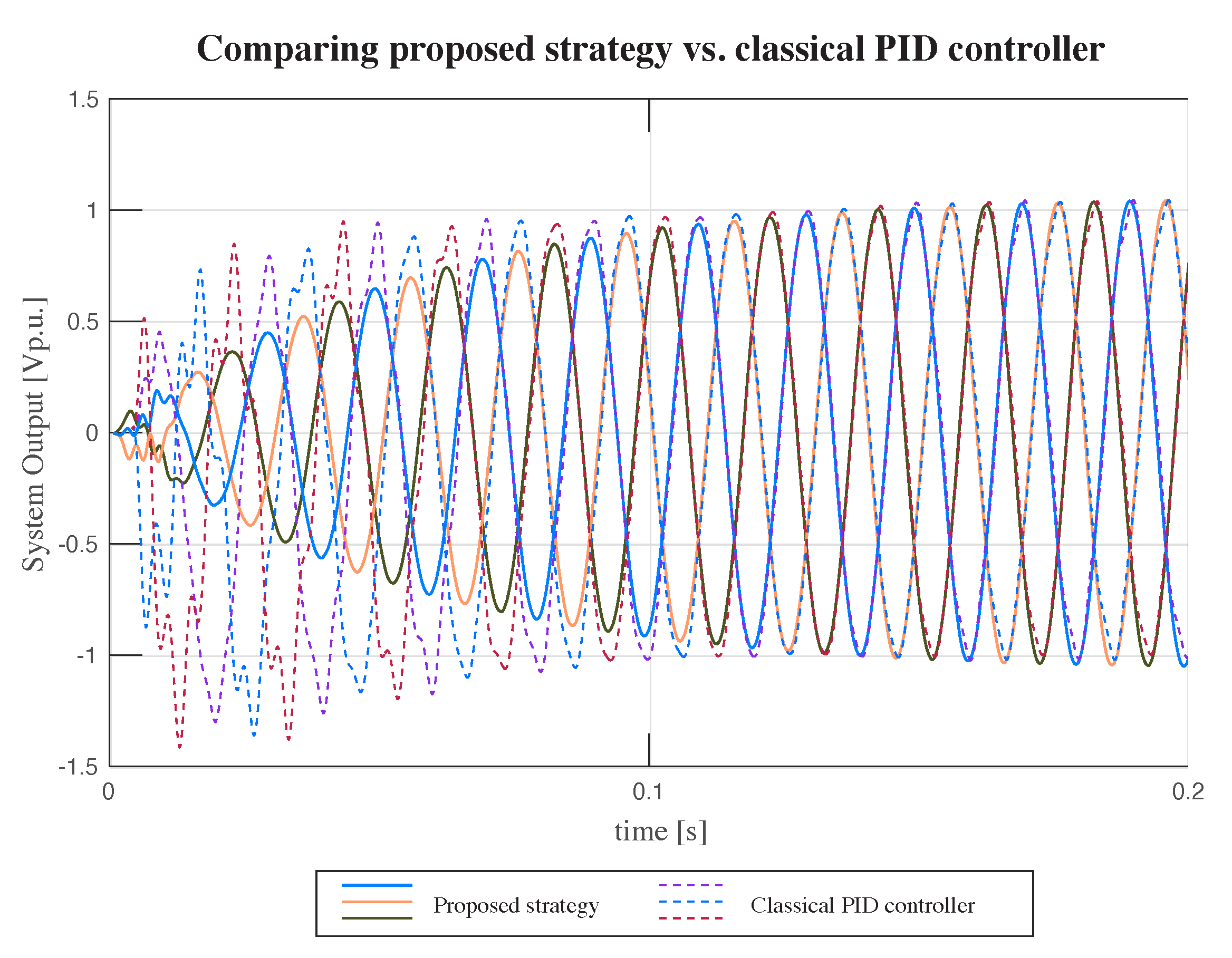
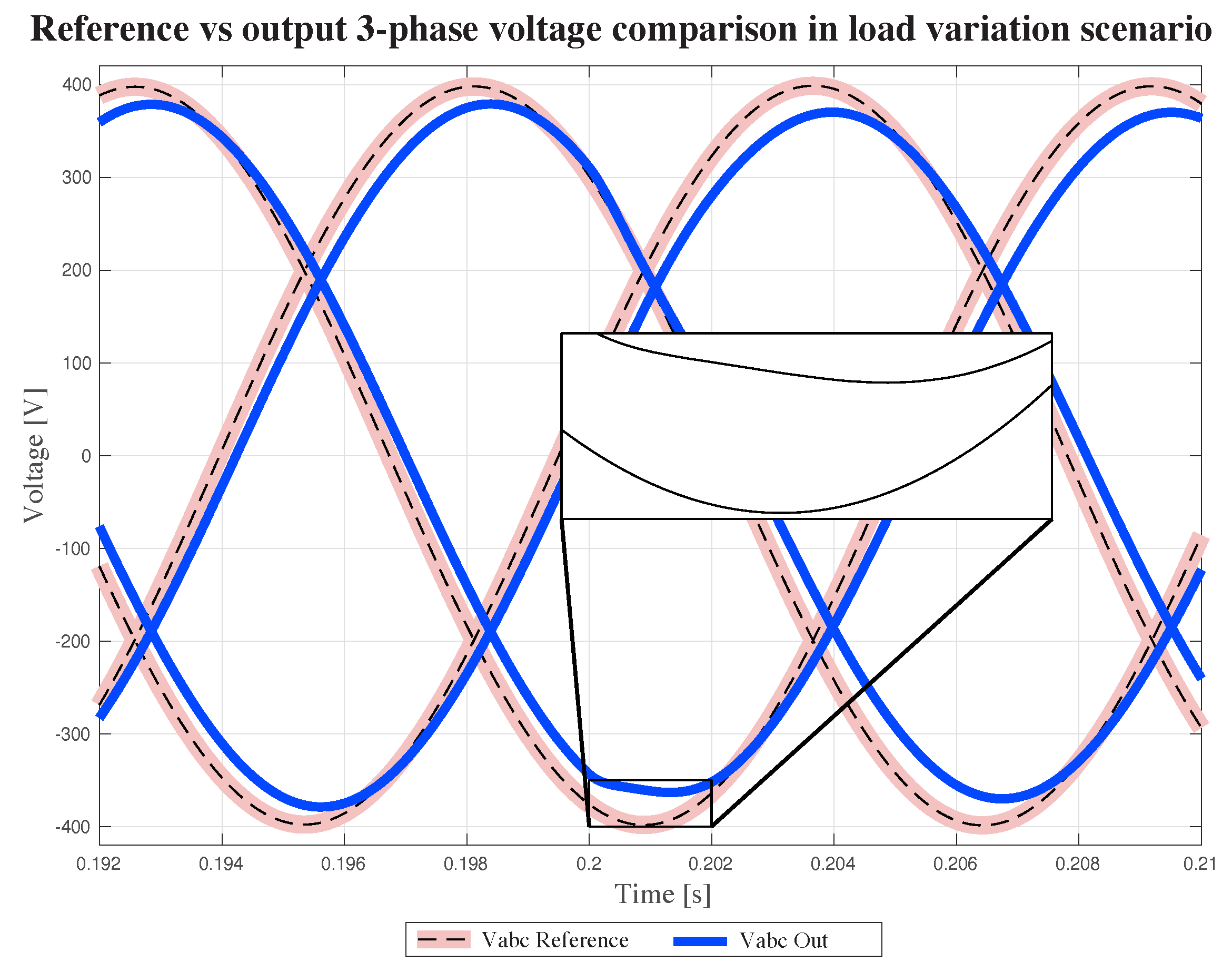
Figure 8 shows the comparison between the three-phase output system voltage, resulting from the proposed methodology, and the performance of a classical PID. It is essential to mention that the second controller can control the output voltage, but it cannot maintain the limit in the current or interchange power between converters. It is seen that the controller is considered stable, and there is not an overshoot due to an over-damped response. The performance in general terms is better than the controller, without considering the advantages in another control level. Additionally, Figure 9 compares the reference signal vs. output voltages with the proposed strategy classical PID controller.

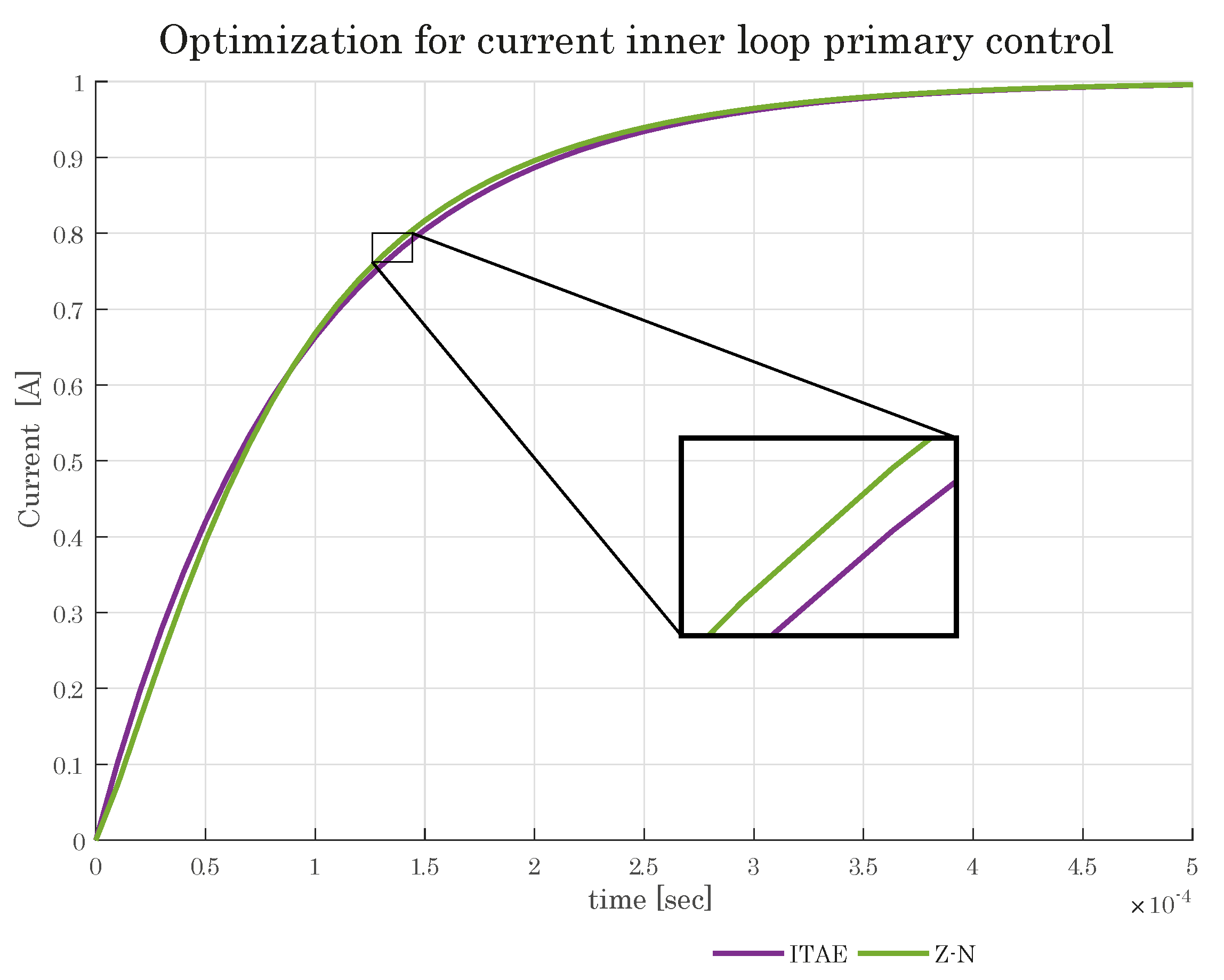
The optimization algorithm’s outcomes for the primary loop are displayed in Figure 10 and Figure 11. Figure 10 presents five system responses, each corresponding to a PID controller calculated using the Integral Time Square Error (ITSE) and Integral Time-weighted Absolute Error (ITAE). The goal of each strategy is to determine the controller coefficients that produce the lowest steady-state error in the system. While the Integral Square Error (ISE), Integral Absolute Error (IAE), and Ziegler and Nichols (ZN) methods are upon each other in down the ITAE line.

The five optimization approaches—ISE, IAE, ITSE, ITAE, and ZN—each consider a step input, as shown in Figure 10 and Figure 11. The system reaches the step input within $4.5\times {10}^{-4}$ [s] and has an over-damped response, with no overshoot. The comparison of the four methodologies and the ZN approach is highlighted in a magnified square, where the highest differences are noted. The ZN method serves as the starting point for the optimization procedures by providing the initial values.

Additionally, the values of the optimization indices are presented in a clear and concise manner in

Table 4. Minimization results for the current loop.

Methodology	Value
ITSE	$1.15\times {10}^{-11}$
ITAE	$5.84\times {10}^{-11}$
ISE	$1.81\times {10}^{-6}$
IAE	$6.09\times {10}^{-6}$

. The table is arranged such that the methods are sorted according to the minimum value they achieve. After evaluating the results, it can be concluded that the ITSE approach is the most effective strategy for finding the smallest error in the steady state for the current control loop. This is particularly important as a small steady state error is crucial for ensuring accurate control of the system.

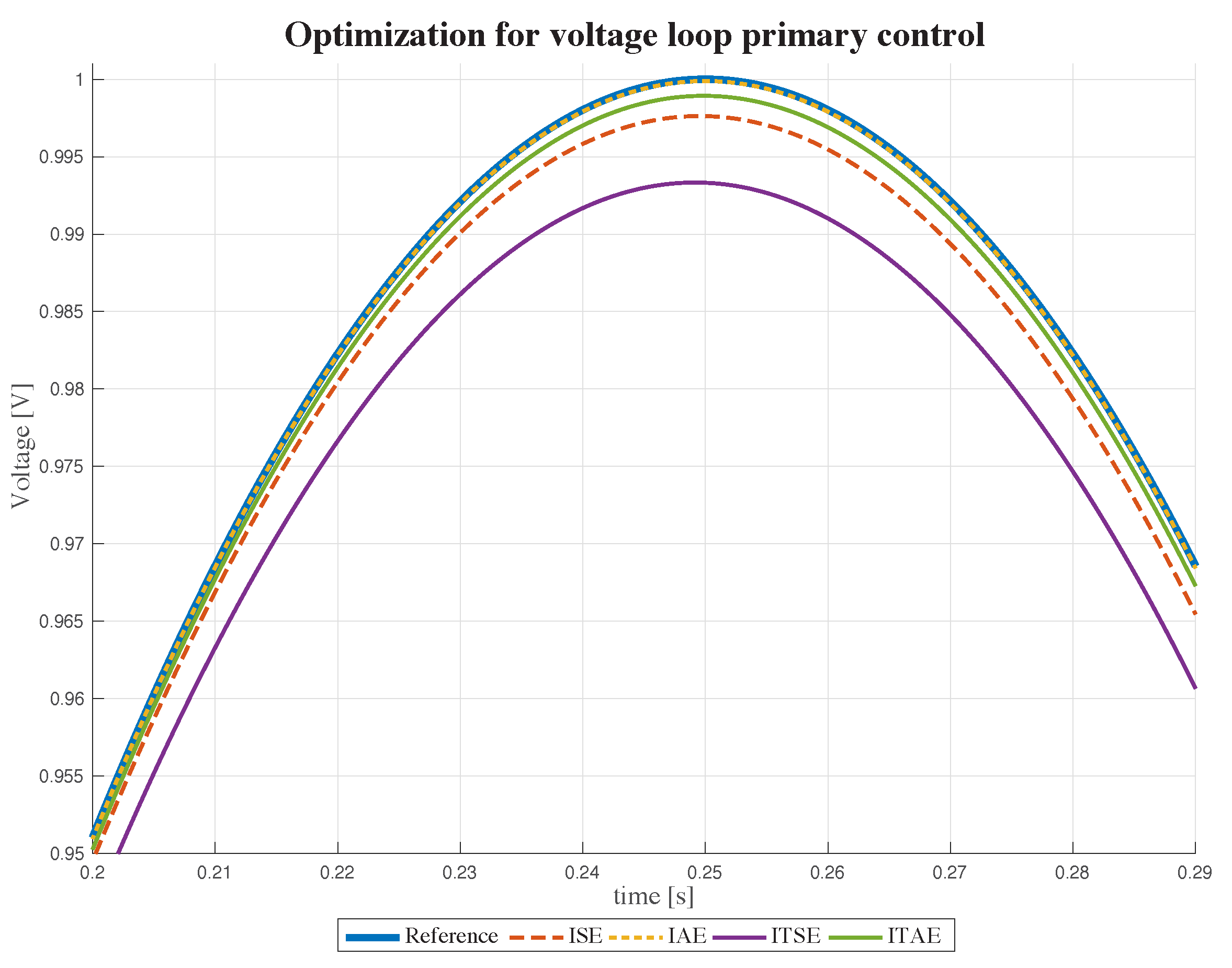
The voltage closed-loop response, fed by a 60 [Hz] sinusoidal input, is displayed in Figure 11 and controlled by the PR approach. The ZN method was not used because the current does not correspond to any magnitude margin, thus there is no resonant constant to derive the initial values for the algorithm. However, the methodology employs random values as an initial guess in the controller optimization calculation, and the algorithm should find the same values as the optimal parameters.

The comparison of the ISE, IAE, ITSE and ITAE methods was made with a sinusoidal reference. It can be seen that there is a significant discrepancy between the reference and ITSE. The evaluation of the objective functions is presented in

Table 5. Minimization results for the voltage loop.

Methodology	Value
IAE	$5.84\times {10}^{-5}$
ITAE	$9.32\times {10}^{-5}$
ISE	$2.50\times {10}^{-4}$
ITSE	$7.31\times {10}^{-4}$

, with ITSE resulting in the least effectiveness.

The ISE and ITAE methods are closest to the reference, with a slight difference in the reference peak. However, the evaluation of the objective function shows satisfactory results. Ultimately, the IAE approach proves to be the best in the experiments, with no significant difference observed between the reference and the controller optimized using IAE.

The results of the function minimization for the voltage loop control are presented in Table 5, ordered from the smallest value. According to the results, IAE optimization is the best method for voltage loop control. The phase margin for the current and voltage loops can be calculated at 0 (rad/s) and 60 (rad/s), respectively. However, the magnitude margin can only be determined for the voltage loop, which affects the algorithm. As a result, the initial values for the optimization algorithm are based on randomly chosen values.

The aim of the secondary control level is to set the voltage and frequency reference values for the primary level and to decrease the circulating current caused by non-linear elements. It regulates the flow of energy throughout the entire Microgrid by balancing the generation and consumption.

The interconnection and relationships among the VSI are considered in this section.

Table 6. Parameters for secondary and tertiary control.

Parameter	Symbol	Value
Proportional gain for controller	$K_e$	7
Drop coefficient for P power control	n	0.21
Drop coefficient for P power control	$n_d$	0.003
Drop coefficient for Q power control	m	$160\mu$
Drop coefficient for Q power control	$m_d$	$2\mu$
P gain for voltage deviation	$k_{pE}$	1.82
I gain for voltage deviation	$k_{iE}$	4.29
P gain for frequency deviation	$k_{p\omega }$	2.23
I gain for frequency deviation	$k_{i\omega }$	7.68

summarizes the values for the secondary control level. The methodology for calculating the parameters was discussed in a previous section and the mathematical relations were also mentioned and referenced. There are two controllers, one for active power P control and the other for reactive power Q control, both of which incorporate a PI controller. The PI regulator parameters for P power control are $k_{pE}$ and $k_{iE}$, while for Q power control they are $k_{p\omega }$ and $k_{i\omega }$.

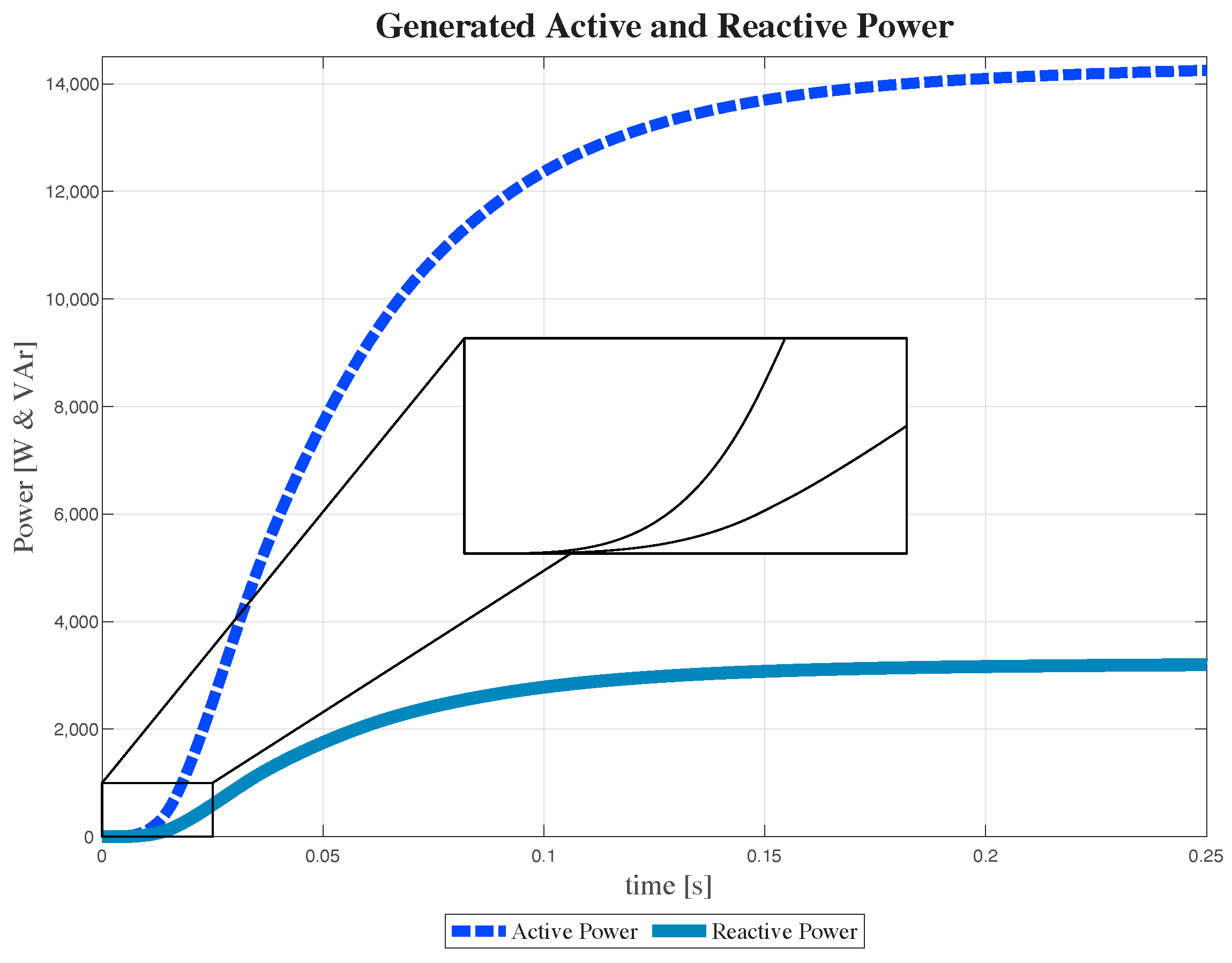
The parameters for droop control are split into P and Q control, with the constants n and $n_d$ for P control and m and $m_d$ for Q control. The proportional constant $K_e$ is used to compensate for voltage variations and its impact on the final results. The active and reactive power generated by a generator in standalone mode are depicted in Figure 12. Initially, the signals are the same, but they exhibit a changing transient behavior. After 0.01 (s), both models exhibit a response that follows a second-order system. The signals reach a maximum point around 0.25 s, then follow their individual references of 375 (W) and 220 (VAr), respectively. In the standalone case, the source responds to the load power, which is not perfectly linear, and includes capacity and inductance elements to provide an imaginary part of power.

4. Conclusions and Future Works

This paper proposes a strategy for controlling an electrical substation of a smart grid with photovoltaic generation, adopting an optimal approach for network layout and control. It relies on a heuristic approach and hierarchical control and involves a design based on optimization for reducing the network length and steady-state error. The plant under study affects a complex nonlinear behavior, and a classical controller might not control this system. Power electronics have multiple nonlinear components, and the photovoltaic generation is unpredictable and changeable.

The microgrid control system strategy follows a hierarchical control architecture, where the primary control system (PCS), also known as the hierarchical control system (HCS), is responsible for controlling the current and voltage outputs. Meanwhile, the secondary control system regulates the voltage amplitude and frequency, which serve as the reference for the desired active and reactive power. This two-tiered control approach allows for effective and efficient control of the microgrid system.

The system’s response is steady and predictable, with a dampened behavior that does not result in over-shooting. Despite the presence of 5% oscillations around the target voltage level, these fluctuations are consistent and maintain a uniform pattern. The response time of the system is quick, taking into account the nonlinear elements and the complex interactions between different components. The time taken for the system to reach its steady state is under 0.4 s, even with an increase in load. This demonstrates the system’s ability to fulfill the power and voltage requirements despite changes in the operating conditions.

The implemented control strategy is often too conservative, as it involves classical controllers for each loop, as proportional integral derivative and proportional resonant, and performance in the case of a more complicated combination of smart grids. The result induces future considerations about introducing distributed generation, smart grid, and photovoltaic installations. Future research will discuss the secondary loop results, including the strategy for optimal parameter tuning. Additionally, the proposed strategy guarantees the system performance in the case of a more complicated combination of smart grids. Additionally, future papers will include metrics related to the power quality issues such as THD to prove that the proposed control system is more efficient.

References

- Pourbehzadi, M.; Niknam, T.; Aghaei, J.; Mokryani, G.; Shafie-khah, M.; Catalão, J.P.S. Optimal operation of hybrid AC/DC microgrids under uncertainty of renewable energy resources: A comprehensive review. Int. J. Electr. Power Energy Syst. 2019, 109, 139–159. [Google Scholar] [CrossRef]
- Ahmethodzic, L.; Music, M. Comprehensive review of trends in microgrid control. Renew. Energy Focus 2021, 38, 84–96. [Google Scholar] [CrossRef]
- Ortiz, L.; Orizondo, R.; Águila, A.; González, J.W.; López, G.J.; Isaac, I. Hybrid AC/DC microgrid test system simulation: Grid-connected mode. Heliyon 2019, 5, e02862. [Google Scholar] [CrossRef] [PubMed] [Green Version]
- Ahmed, M.N.; Hojabri, M.; Humada, A.M.; Daniyal, H.B.; Fahad Frayyeh, H. An Overview on Microgrid Control Strategies. Int. J. Eng. Adv. Technol. IJEAT 2015, 4, 93–98. [Google Scholar]
- Unamuno, E.; Barrena, J.A. Hybrid ac/dc microgrids - Part I: Review and classification of topologies. Renew. Sustain. Energy Rev. 2015, 52, 1251–1259. [Google Scholar] [CrossRef]
- Zolfaghari, M.; Gharehpetian, G.B.; Shafie-khah, M.; Catalão, J.P.S. Comprehensive review on the strategies for controlling the interconnection of AC and DC microgrids. Int. J. Electr. Power Energy Syst. 2022, 136, 107742. [Google Scholar] [CrossRef]
- Lee, D.; Wang, L. Small-Signal Stability Analysis of an Autonomous Hybrid Renewable Energy Power Generation/Energy Storage System Part I: Time-Domain Simulations. IEEE Trans. Energy Convers. 2008, 23, 311–320. [Google Scholar] [CrossRef]
- Yepez, H.; Pavon, W.; Simani, S.; Ayala, E.; Asiedu-Asante, A.B. Source Inverter Voltage and Frequency Control for AC Isolated Microgrid Applications. In Proceedings of the 2022 IEEE 7th International Energy Conference (ENERGYCON), Riga, Latvia, 9–12 May 2022; pp. 1–6. [Google Scholar] [CrossRef]
- Hirsch, A.; Parag, Y.; Guerrero, J. Microgrids: A review of technologies, key drivers, and outstanding issues. Renew. Sustain. Energy Rev. 2018, 90, 402–411. [Google Scholar] [CrossRef]
- Pavon, W.; Inga, E.; Simani, S.; Nonato, M. A Review on Optimal Control for the Smart Grid Electrical Substation Enhancing Transition Stability. Energies 2021, 14, 8451. [Google Scholar] [CrossRef]
- Irfan, M.; Iqbal, J.; Iqbal, A.; Iqbal, Z.; Riaz, R.A.; Mehmood, A. Opportunities and challenges in control of smart grids—Pakistani perspective. Renew. Sustain. Energy Rev. 2017, 71, 652–674. [Google Scholar] [CrossRef]
- Sen, S.; Kumar, V. Microgrid modelling: A comprehensive survey. Annu. Rev. Control 2018, 46, 216–250. [Google Scholar] [CrossRef]
- Lema, M.; Pavon, W.; Ortiz, L.; Asiedu-Asante, A.B.; Simani, S. Controller Coordination Strategy for DC Microgrid Using Distributed Predictive Control Improving Voltage Stability. Energies 2022, 15, 5442. [Google Scholar] [CrossRef]
- Pavón, W.; Inga, E.; Simani, S.; Armstrong, M. Novel Single Stage DC/AC Power Inverter for a Standalone Photovoltaic System Controlled by a Double Loop Scheme. In Proceedings of the 2022 IEEE 10th International Conference on Smart Energy Grid Engineering (SEGE), Oshawa, ON, Canada, 10–12 August 2022; pp. 111–118. [Google Scholar] [CrossRef]
- Twaha, S.; Ramli, M.A.M. A review of optimization approaches for hybrid distributed energy generation systems: Off-grid and grid-connected systems. Sustain. Cities Soc. 2018, 41, 320–331. [Google Scholar] [CrossRef]
- Vallejos, W.D.P. Standalone photovoltaic system, using a single stage boost DC/AC power inverter controlled by a double loop control. In Proceedings of the 2017 IEEE PES Innovative Smart Grid Technologies Conference—Latin America (ISGT Latin America), Quito, Ecuador, 20–22 September 2022; pp. 1–6. [Google Scholar] [CrossRef]
- Planas, E.; Gil-de Muro, A.; Andreu, J.; Kortabarria, I.; Martínez de Alegría, I. General aspects, hierarchical controls and droop methods in microgrids: A review. Renew. Sustain. Energy Rev. 2013, 17, 147–159. [Google Scholar] [CrossRef]
- Planas, E.; Andreu, J.; Gárate, J.I.; Martínez De Alegría, I.; Ibarra, E. AC and DC technology in microgrids: A review. Renew. Sustain. Energy Rev. 2015, 43, 726–749. [Google Scholar] [CrossRef]
- Hossain, E.; Kabalci, E.; Bayindir, R.; Perez, R. Microgrid testbeds around the world: State of art. Energy Convers. Manag. 2014, 86, 132–153. [Google Scholar] [CrossRef]
- Olivares, D.E.; Mehrizi-Sani, A.; Etemadi, A.H.; Cañizares, C.A.; Iravani, R.; Kazerani, M.; Hajimiragha, A.H.; Gomis-Bellmunt, O.; Saeedifard, M.; Palma-Behnke, R.; et al. Trends in microgrid control. IEEE Trans. Smart Grid 2014, 5, 1905–1919. [Google Scholar] [CrossRef]
- Nutkani, I.U.; Loh, P.C.; Wang, P.; Jet, T.K.; Blaabjerg, F. Intertied ac–ac microgrids with autonomous power import and export. Int. J. Electr. Power Energy Syst. 2015, 65, 385–393. [Google Scholar] [CrossRef]
- Eghtedarpour, N.; Farjah, E. Power Control and Management in a Hybrid AC/DC Microgrid. IEEE Trans. Smart Grid 2014, 5, 1494–1505. [Google Scholar] [CrossRef]
- Campaña, M.; Masache, P.; Inga, E.; Carrión, D. Estabilidad de tensión y compensación electrónica en sistemas eléctricos de potencia usando herramientas de simulación. Ingenius 2022, 2. [Google Scholar] [CrossRef]
- Li, Z.; Zheng, T.; Wang, Y.; Yang, C. A Hierarchical Coordinative Control Strategy for Solid State Transformer Based DC Microgrids. Appl. Sci. 2020, 10, 6853. [Google Scholar] [CrossRef]
- Wang, G.; Wang, X.; Wang, F.; Han, Z. Research on Hierarchical Control Strategy of AC/DC Hybrid Microgrid Based on Power Coordination Control. Appl. Sci. 2020, 10, 7603. [Google Scholar] [CrossRef]
- Wang, C.; Minjian, C.; Martínez, L.R. Design of load optimal control algorithm for smart grid based on demand response in different scenarios. Open Phys. 2018, 16, 1046–1055. [Google Scholar] [CrossRef]
- Wang, J.; Jin, C.; Wang, P. A Uniform Control Strategy for the Interlinking Converter in Hierarchical Controlled Hybrid AC/DC Microgrids. IEEE Trans. Ind. Electron. 2018, 65, 6188–6197. [Google Scholar] [CrossRef]
- Unamuno, E.; Barrena, J.A. Hybrid ac/dc microgrids—Part II: Review and classification of control strategies. Renew. Sustain. Energy Rev. 2015, 52, 1123–1134. [Google Scholar] [CrossRef]
- Hosseinzadeh, M.; Salmasi, F.R. Power management of an isolated hybrid AC/DC micro-grid with fuzzy control of battery banks. IET Renew. Power Gener. 2015, 9, 484–493. [Google Scholar] [CrossRef]
- Antoniadou-Plytaria, K.E.; Kouveliotis-Lysikatos, I.N.; Georgilakis, P.S.; Hatziargyriou, N.D. Distributed and Decentralized Voltage Control of Smart Distribution Networks. IEEE Trans. Smart Grid 2017, 8, 2999–3008. [Google Scholar] [CrossRef]
- Palizban, O.; Kauhaniemi, K. Hierarchical control structure in microgrids with distributed generation: Island and grid-connected mode. Renew. Sustain. Energy Rev. 2015, 44, 797–813. [Google Scholar] [CrossRef]
- Ziouani, I.; Boukhetala, D.; Darcherif, A.M.; Amghar, B.; El Abbassi, I. Hierarchical control for flexible microgrid based on three-phase voltage source inverters operated in parallel. Int. J. Electr. Power Energy Syst. 2018, 95, 188–201. [Google Scholar] [CrossRef]
- Teodorescu, R.; Blaabjerg, F.; Liserre, M.; Loh, P.C. Proportional-resonant controllers and filters for grid-connected voltage-source converters. IEE Proc. Electr. Power Appl. 2006, 153, 750–762. [Google Scholar] [CrossRef] [Green Version]
- González-Castaño, C.; Restrepo, C.; Giral, R.; Vidal-Idiarte, E.; Calvente, J. ADC Quantization Effects in Two-Loop Digital Current Controlled DC-DC Power Converters: Analysis and Design Guidelines. Appl. Sci. 2020, 10, 7179. [Google Scholar] [CrossRef]
- Wang, Q.; Zuo, W.; Cheng, M.; Deng, F.; Buja, G. Hierarchical control with fast primary control for multiple single-phase electric springs. Energies 2019, 12, 3511. [Google Scholar] [CrossRef] [Green Version]
- Visioli, A. A new design for a PID plus feedforward controller. J. Process Control 2004, 14, 457–463. [Google Scholar] [CrossRef]
- Lorenzini, C.; Bazanella, A.S.; Pereira, L.F.A.; Gonçalves da Silva, G.R. The generalized forced oscillation method for tuning PID controllers. ISA Trans. 2019, 87, 68–87. [Google Scholar] [CrossRef]
- Levine, S.; Koltun, V. Continuous Inverse Optimal Control with Locally Optimal Examples. In Proceedings of the International Conference on Machine Learning (ICML), Edinburgh, UK, 26 June–1 July 2012. [Google Scholar]
- Pereira, L.F.A.; Bazanella, A.S. Tuning Rules for Proportional Resonant Controllers. IEEE Trans. Control Syst. Technol. 2015, 23, 2010–2017. [Google Scholar] [CrossRef]
- Pinzón, S.; Pavón, W. Diseño de Sistemas de Control Basados en el Análisis del Dominio en Frecuencia. Revista Técnica “Energía” 2019, 15, 76–82. [Google Scholar] [CrossRef] [Green Version]
- Wang, X.; Lv, H.; Sun, Q.; Mi, Y.; Gao, P. A Proportional Resonant Control Strategy for Efficiency Improvement in Extended Range Electric Vehicles. Energies 2017, 10, 204. [Google Scholar] [CrossRef] [Green Version]
- Marín, L.G.; Sumner, M.; Muñoz-Carpintero, D.; Köbrich, D.; Pholboon, S.; Sáez, D.; Núñez, A. Hierarchical Energy Management System for Microgrid Operation Based on Robust Model Predictive Control. Energies 2019, 12, 4453. [Google Scholar] [CrossRef] [Green Version]
- Zhong, Q.; Zeng, Y. Universal Droop Control of Inverters with Different Types of Output Impedance. IEEE Access 2016, 4, 702–712. [Google Scholar] [CrossRef]
Figure 1.
AC/DC hybrid microgrid integrating Renewable Energy Systems generators and AC loads.
Figure 2.
Controller structure for primary control.
Figure 3.
Primary control block diagram, including voltage and current structure.
Figure 4.
Droop control controlling active and reactive power.
Figure 5.
Block diagram for the secondary control.
Figure 6.
Comparing the reference voltage with the voltage output inverter.
Figure 7.
Comparing the RMS reference voltage output and the RMS output voltage inverter.
Figure 8.
Comparing 3-phase output voltage of the proposed strategy vs. classical PID controller, in per-unit values.
Figure 9.
Comparing reference signal vs. output voltages with proposed strategy classical PID controller.
Figure 10.
The optimization techniques for the current inner loop of the primary control are compared.
Figure 11.
Optimization techniques for voltage inner loop primary control are compared.
Figure 12.
Active and reactive power from the inverter is delivered to the stand-alone load.