
Simulation of Polymer Chemical Enhanced Oil Recovery in Ghawar Field

Department of Chemical Engineering, ENTEG, University of Groningen, Nijenborgh 4, 9747 AG Groningen, The Netherlands
*
Author to whom correspondence should be addressed.
†
These authors contributed equally to this work.
Energies 2022, 15(19), 7232; https://doi.org/10.3390/en15197232
Submission received: 31 August 2022
/
Revised: 21 September 2022
/
Accepted: 26 September 2022
/
Published: 1 October 2022
(This article belongs to the Special Issue Heat Transfer and Mathematical Modeling of Multi-Phase Flow through Porous Media)
Abstract
:This paper presents a 2D model of the Ghawar field and investigates the flow behavior in the field during secondary and tertiary recoveries using a simplified well scheme. For the latter, the focus is on chemical Enhanced Oil Recovery (EOR), using polymer solutions. The difference in efficiency between secondary and tertiary recovery and the influence of factors such as degradation are analyzed and presented. Furthermore, the influence of oil viscosity on the recovery factor is investigated as well as the efficiency of the well placement of the model studied. In order to do this, a combined shear-thinning/-thickening model, the Unified Viscosity Model (UVM), is used. COMSOL Multiphysics is used in order to study the model, combining the fluid flow and mass transfer in one study, showing the interdependence of both physics transport phenomena. The results show how the influence of the polymer properties and the rock formation affect the recovery behavior. The particle tracing study allows us to determine the percentage of the chemical agent recovered in the producing wells. This paper shows how EOR agents works coupled with advanced numerical models in real-scale fields.
1. Introduction
During the last 150 years, oil has become the world’s main source of energy, and its production has been steadily increasing, reaching more than 30 billion barrels per year at the beginning of the current century [1,2,3] and playing nowadays a large role in the world economy and politics [4]. Though more sustainable energy sources are being developed in order to replace hydrocarbons, they cannot replace it at the moment. This leads to two different outcomes: either finding new oilfields or improving the usage of the known ones. Chemical Enhanced Oil Recovery aims at the second, and the synthesis and test of new agents, such as polymers, has shown potential in its limited field application [5,6]. There are several techniques to recover oil from reservoirs, classified by the energy source behind oil recovery. An overview of the classification of techniques are given in Figure 1 [5]. Oil recovery by primary techniques relies on the natural pressure gradient present in the reservoir and is driven by internal energy [7,8]. As a result of the oil production, the pressure decreases. Secondary techniques are used to re-pressurize the reservoir and increase production (e.g., waterflooding). Waterflooding is a relatively inexpensive technique to recover oil since water is generally available in large quantities [9]. However, the percentage of oil recovered by using primary and secondary techniques is only around 35–55% of the Original Oil In Place (OOIP) [9,10,11,12]. The oil viscosity influences the recovery factor. Water can easily displace low-viscosity oil by forming a stable flood front. However, when the oil is more viscous, water has the tendency to finger through the oil, and water breakthrough occurs in an early stage [12].
EOR is focused on extracting oil that is left behind [7] and includes the injection of chemicals, heat and/or miscible gases into the reservoir, making it possible to extract up to an additional 30% of the OOIP [13]. The interest in EOR is increasing due to the difficulty of discovering new oil fields coupled with the slightly decreasing reserves-to-production (R/P) ratio (53.5 years in 2020) and increasing oil consumption [14]. The R/P ratio indicates the time that the recoverable oil, which is still present in discovered oil fields, will last if production continues at the production rate of the previous year.
Chemical EOR (cEOR) is one of the most promising methods within EOR. This method involves the use of various chemicals, mostly injected into the reservoir in the form of diluted solutions [15,16]. Within cEOR, the use of aqueous polymer solutions, also named polymer flooding, is the most mature and important method [17]. Water-soluble polymers can be used alone or in combination with surfactants, nanoparticles and/or an inorganic base. Polymers have the purpose of increasing the viscosity of the displacing fluid and thereby decreasing the water/oil mobility ratio. This leads to an increased sweep and displacement efficiency. Furthermore, polymer solutions exhibit viscoelastic behavior when flowing through porous media. Channels in porous media are converging/diverging, which accelerates and subsequently decelerates the flow. Entering the converging section of a pore channel, the shear rate increases and the polymer elongation in the direction of the flow occurs, which results in an increase in viscosity and enhanced displacement. Furthermore, elongation of the polymers results in enhanced microscopic displacement in pore channels by extracting oil from dead ends and the rock surface [18]. Moreover, the retention of polymers within the field should be as low as possible since this phenomenon significantly influences the oil recovery rate and economic feasibility of cEOR [13]. This is mainly caused by adsorption and mechanical entrapment. It is well-known that in carbonate reservoirs, such as Ghawar, the retention of the commonly used polymers in EOR is much higher than in sandstones. The retention investigated in this paper, however, is due to the physical location of the wells, their pattern, and the velocity field developed in the rock formation, causing that part of the molecule to remain underground without going to the producer wells. The study of the polymer retention processes is advised for future developments.
Aim of This Work
A comprehensive reservoir characterization and two-dimensional simulation are made for the Ghawar oilfield, simulating the flow of a two-phase, three-component system. The goal is to investigate the flow behavior in the field during secondary and cEOR polymer flooding. The difference in efficiency between secondary and tertiary recovery, as well as the influence of the degradation, will be analyzed. The non-Newtonian polymer behavior is also considered, using a shear-thinning and -thickening model. For this research, it was chosen to investigate the above-mentioned factors using the simulation package COMSOL Multiphysics. In this case, the water viscosity is indeed affected by the polymer concentration. Finally, we consider in a novel way the effect of the polymer flooding on the residual oil saturation by modifying the relative permeability curve, which, to our best knowledge, has not been considered in previous academic simulators.
2. Model Description
2.1. Physical Model
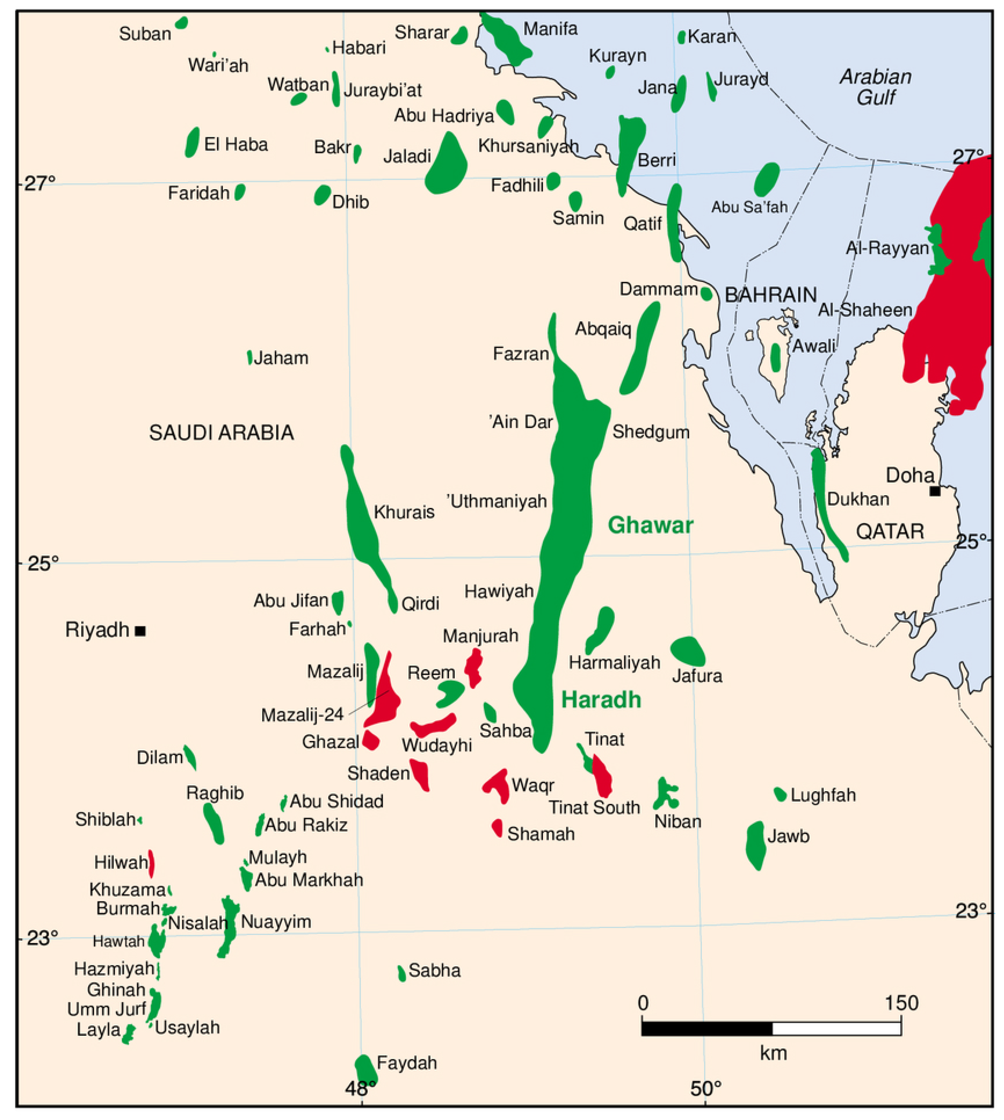
The Ghawar oil field (Figure 2), located in Saudi Arabia, is the largest oil reservoir in the world [19]. The field is situated on the southern part of the En Nala anticline and is around 245 km long, 25 km wide and 90 m thick [20,21]. It covers an area of 5300 km2 and is divided into six parts based on production, namely from north to south: Fazran, Ain Dar, Shedgum, Uthmaniyah, Haradh and Hawiyah. Saudi Aramco discovered the Ghawar field in 1948, and production started in 1951. In 1981, production reached a peak of 5.7 MMbbl per day, the highest oil production achieved by a single field in world history. At that time, the southern areas, Hawiyah and Haradh were not fully developed yet. After 1981, production decreased for economic reasons [22]. The remaining proved oil reserve of the Ghawar field was estimated on 58.3 billion barrels oil equivalent (Gbbl) in 2019 and has a production capacity of 3.8 million barrels (MMbbl) per day.
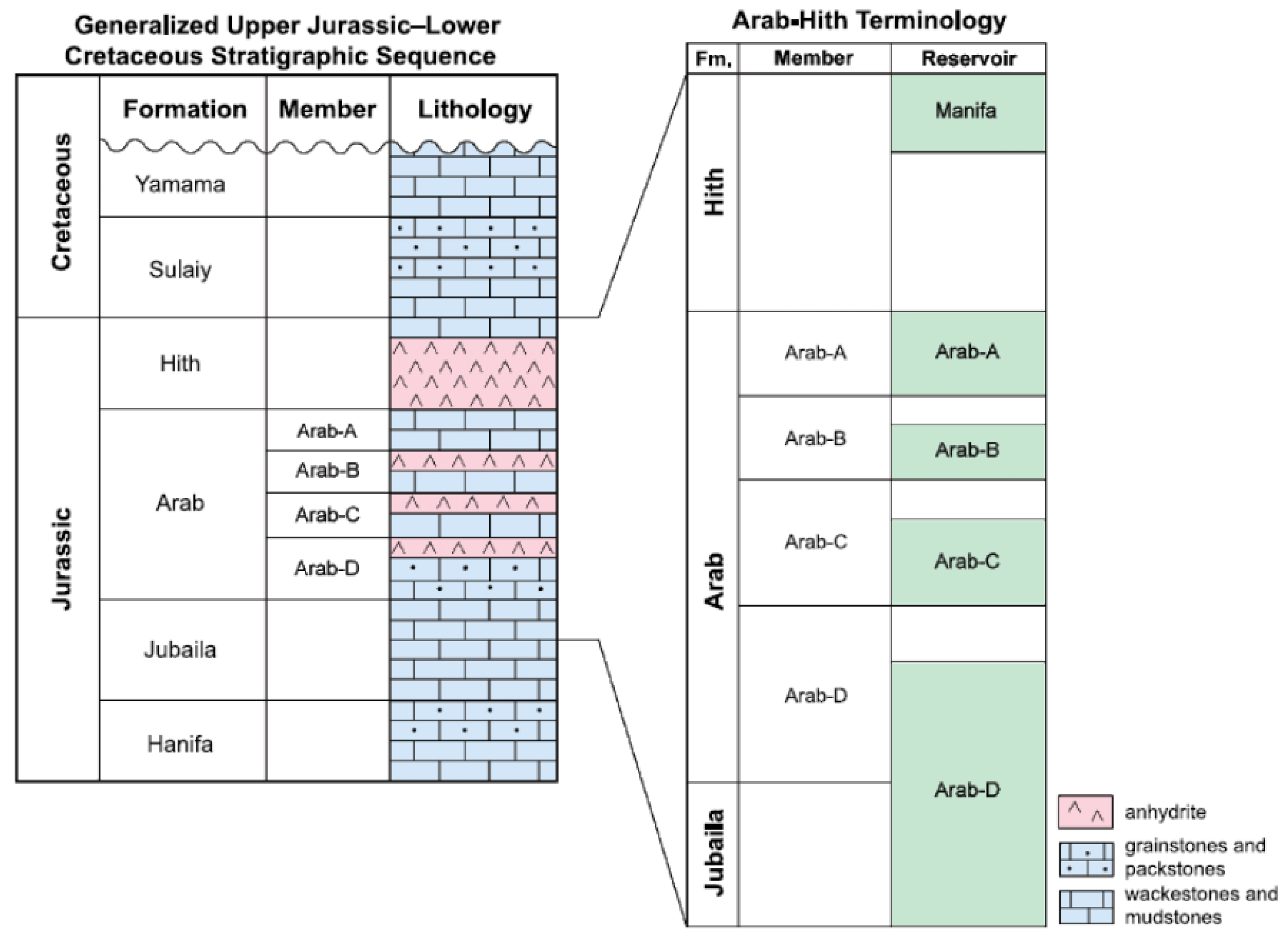
A general overview of the stratigraphy of the Ghawar field is given in Figure 3. The oil reservoir was formed during the Late Jurassic and Early Cretaceous periods. All the oil produced at Ghawar comes from the Arab-D reservoir [23]. The Arab-D reservoir consists of Upper Jurassic dolomites and carbonate rocks, which contain more than 75% of the mineral dolomite. Typically, these rocks are formed during the diagenesis of limestones, which results in a fundamental difference in reservoir characteristics between limestones and dolomites [24,25]. The Arab-D reservoir is sealed by evaporates of Arab C-D anhydrite and topped with Upper Jurassic anhydrite, named Hith anhydrite, which prevents the vertical migration of oil.
It is important to remark that in this first numerical model of the Ghawar oilfield, we have considered and studied only one layer, and regarding the rock formation properties, i.e., porosity and permeability, the heterogeneity of both has been simplified in order to test the numerical behavior of the whole system.
Ghawar’s Arab-D dolomite is responsible for zones with a very high permeability, also called super-k. Super-k areas are defined as areas in which the flow is larger than 500 barrels per day per foot of vertical interval [24]. The dolomite type present in these zones contains moldic porosity and has a high inter-crystalline porosity. The combination of these two types results in high flow and recovery rates. However, these zones also come together with some challenges, and as for secondary recovery, the water flow in the producing wells is also very large [27]. The reservoir quality of the Ghawar field reduces from north to south as the porosity and permeability are significantly lower in the south. Furthermore, the oil quality decreases in the southern area as the density and the oil sulfur content are higher compared to oil in the northern area. The oil density varies over the field between 30 and 34 degAPI and is classified as light to medium oil [19]. In this paper, COMSOL Multiphysics is used to model an enhanced oil recovery process in the Ghawar field. Validation and verification of several studies demonstrated that COMSOL Multiphysics is a reliable simulation environment [28,29].
2.2. Geometry
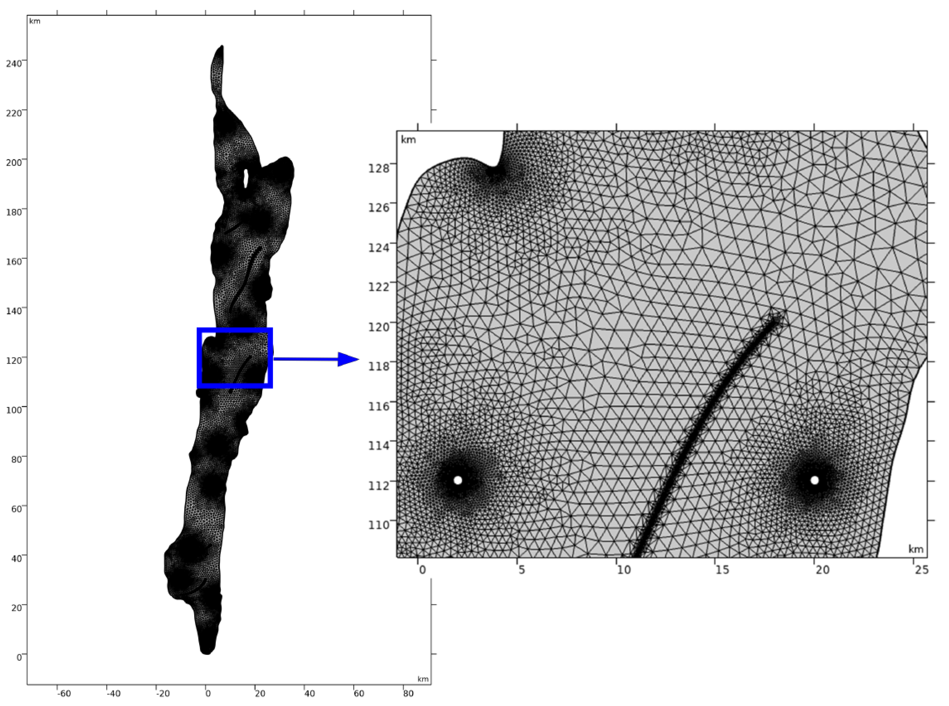
The basis for the numerical simulation was creating the geometry of the Ghawar field. To our knowledge, detailed data on the geometry of the field are not available. Therefore a cartesian coordinate system with 344 data points was created based on Figure 4. Furthermore, the location of impermeable thin-walls was identified by using a figure provided by Lindsay [30] (Figure 5). It was assumed that these walls are located in zones with less than 5% dolomite. These are considered in the model as thin areas in which the flow through cannot take place. However, it is recommended that in future studies, these walls must be replaced by partially permeable areas in order to study the new flow configuration in the oilfield, and these will probably render a new well configuration.
Injectors and Producers
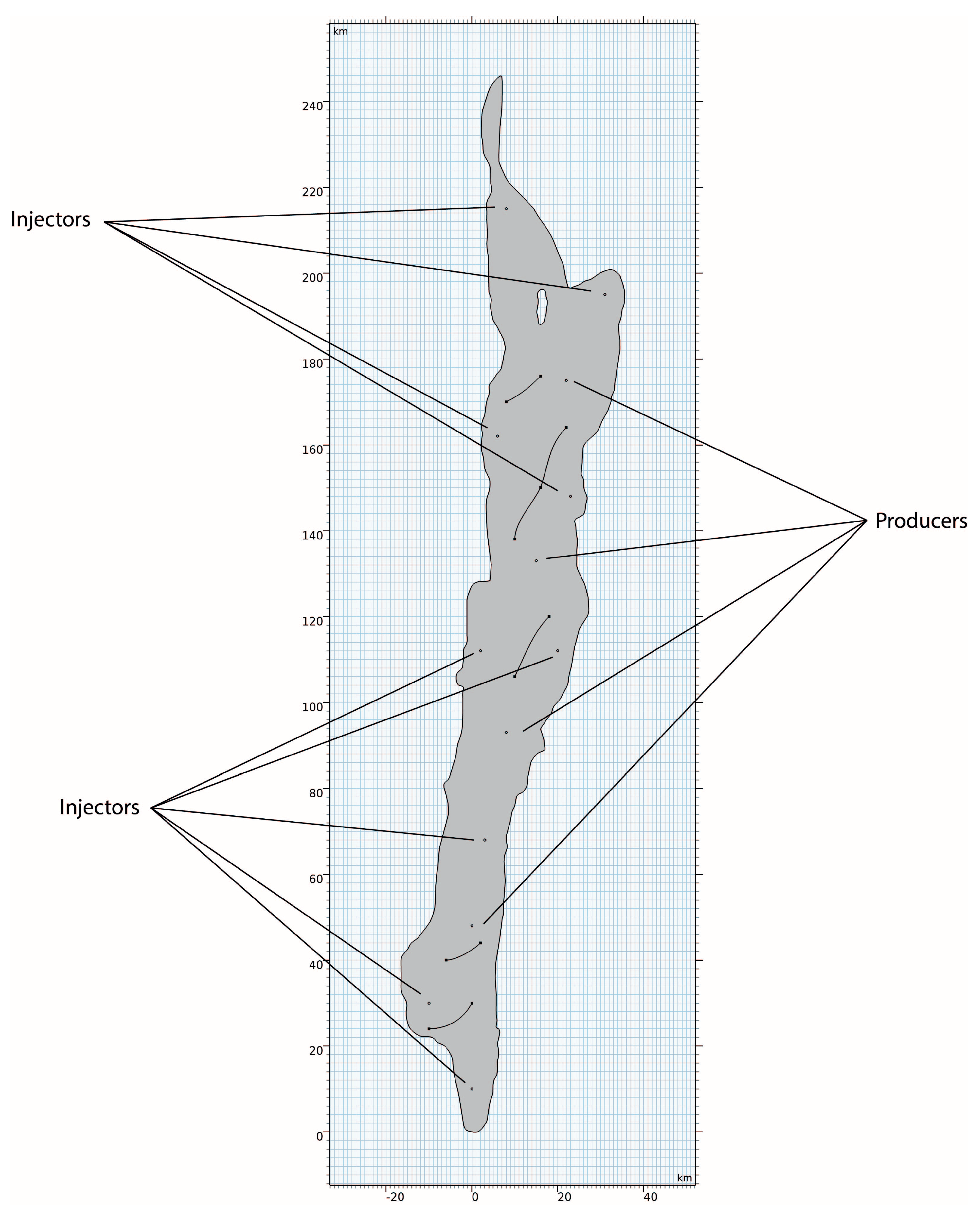
The coordinates were loaded into COMSOL, and interpolation curves were used to construct the 2D model, which is demonstrated in Figure 6. As the field is very large, hundreds of wells had to be modeled to obtain a realistic well scheme. Modeling such a high number of wells in COMSOL was too demanding as this requires high computational power and an extremely dense mesh. Therefore, 14 wells, including 9 injectors and 5 producers, are modeled in COMSOL with a fictitious radius of 0.25 km (see Figure 6). The placement of the wells is based on a well scheme in which one producer well is surrounded by several injection wells. The injection pattern in the northern half of the field resembles a five-spot scheme, whilst in the southern half, the scheme looks like a four-spot system. It is also worth mentioning that the injection scheme in the actual field is peripheral. Indeed, in the southern part of the field, the producer wells are surrounded by a single injection well. This is chosen since the porosity and permeability are relatively low in this area, which reduces the flow ability. Furthermore, the faults inhibit the flow in this area, which resulted in the placement of two producer wells instead of one to improve the recovery in this area. This modification of the dimensions of real wells was made only for the purposes of the simulation of an oilfield such as Ghawar, also considering numerical constraints. It is deemed that in the future, more developed models with more accurate dimensions should be developed, and simulations should be performed in order to validate the approach followed by our model in Comsol.
The well’s radii and their quantity differ, of course, from the actual values commonly found in the field and this is expected to produce exploitation times, which are much shorter than those found in the industry. The reason for this is purely numerical: by selecting wells with the proper size and amount, the simulation times and complexity should be much longer, and at this first stage of the simulation, the goal was to model the system and study how the polymer would flow in the reservoir. Future studies of this model should contemplate the actual sizes and quantities, which will render more realistic exploitation times.
2.3. Porosity and Permeability
The following data were found for the permeability and porosity of the Ghawar field [19]. As can be seen in Table 1, both parameters differ highly from north to south. In order to generate the porosity and permeability field in COMSOL, random and step functions are used. With respect to this, the functions are necessary in COMSOL to make a reasonably smooth transition between the areas, especially with the permeability since the values differ greatly. The random function is added in order to give small, stochastic-in-nature variations and to resemble as much as possible the behavior of the formation. The influence of these random functions may be decreased in the future in case of including more information about the porosity and permeability of the oilfield.
2.4. Mathematical Model
From the fluid flow add-on, the two-phase Darcy’s Law module for fluid flow in porous media was used. Darcy’s Law was used to compute the pressure of the domain. Furthermore, the module determines the velocity field based on the pressure, fluid viscosity and permeability. Moreover, the transport equation for the fluid content is solved [31,32,33,34,35]. The equations describing the flow in the rock formation and the mass transfer are,
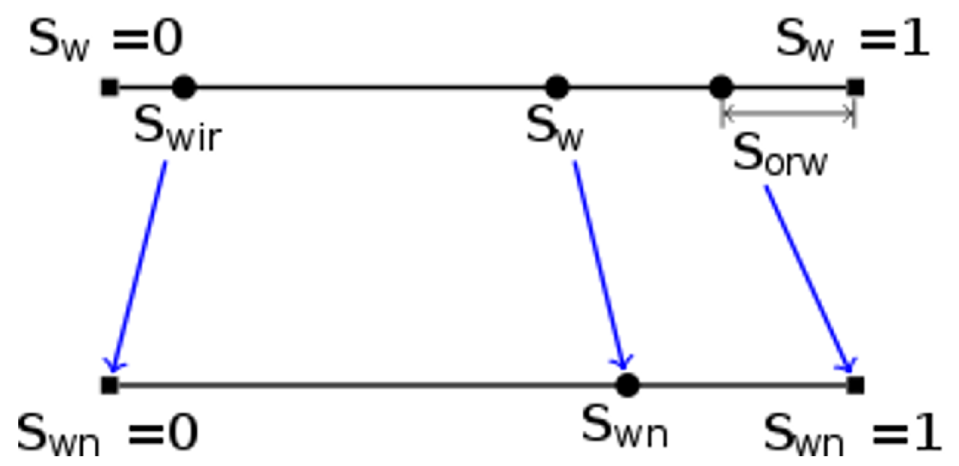
COMSOL works with the concept of effective normalized saturation, which is shown in Figure 7. The software transforms the irreducible water saturation () to a null value, and the residual oil saturation () is assigned a value equal to unity.
For non-Newtonian fluids, the equation for the viscosity is a function of the shear rate. However, the shear rate is calculated by the velocity field, which results in a numerical loop in COMSOL, and this cannot be solved with the selected physics modules. Therefore, a previous simulation with a Newtonian fluid was carried out in order to obtain the shear rate in the oilfield. Subsequently, the shear rate was adapted with this value in the formula for the viscosity. There are several formulas that describe the shear rate in porous media. The formulae described by Sheng were evaluated [36]. These are defined as follows:
where represents the shear rate, is an empirical constant, n the power-law exponent of the fluid, the Darcy velocity of the water phase, K the permeability, the water phase relative permeability and the water saturation.
2.5. Initial and Boundary Conditions
The initial saturation and pressure are defined using values taken from the literature. The oil initial oil saturation is considered to be 0.75 for all the cases simulated. These parameters are assumed to be constant over the whole oilfield. This assumption was made based on standard values found in the industry since no information was obtained on the field’s initial saturation and pressure at the beginning of its exploitation.
During waterflooding, water is injected at a constant rate at the injection wells. The contour of the field and faults are considered as no-flow since these are assumed to consist of impermeable rocks.
2.6. Transport of Diluted Species
The transport of diluted species module in COMSOL provides the option for modeling transport by convection and diffusion of chemical substances. The module assumes that all the chemicals are diluted, which means that the concentration of solvent is higher than 90 mol%. When the substance is diluted, Fick’s Law of diffusion is valid. The governing equation in the transport of diluted species module is the mass balance Equation (2).
The first term in the equation represents the accumulation or consumption of species. The second term concerns the convective transport as a function of the velocity field u, which is obtained from the flow interface (two-phase Darcy’s Law). The diffusion transport involves the interaction between the diluted species and the solvent. The diffusion coefficient can be defined manually in the interface. The source/sink term accounts for the production or consumption of a species by chemical reaction. Reactions can be included in the interface by adding the corresponding node.
The effective diffusion coefficient for the most commonly used polymers in EOR, HPAM (partially hydrolyzed polyacrylamide) and the biopolymer Xanthan gum, in diluted solution is reported to be around [37,38]. One of the main problems with transport in porous media is relating the permeability to experimental data. One of the most well-known formulas for this purpose is the Carman–Kozeny equation [39]. The initial formula developed by Kozeny did not take into account the pore connectivity and was not valid for complex geometries [40]. As streamlines in porous media are tortuous and not parallel to each other, Carman adapted Kozeny’s equation by introducing the concept of tortuosity [41]:
where is the Kozeny constant, is the tortuosity and is the total specific surface area of the porous medium. The tortuosity was defined as the ratio between the flow path length and the straight distance between the flow path ends, which was concluded to be a constant factor for a broad range of porosities [39]. However, further research contradicted this conclusion and demonstrated that the tortuosity depends on the porosity. The following empirical relationship is used to describe the flow in porous media:
Boundary Conditions for Transport of Diluted Species
During polymer flooding, the polymer is injected at a constant concentration at the injection wells. Afterward, water is injected to displace the remaining oil. The contour of the field, and the faults are considered as no flow since these are assumed to consist of impermeable rocks.
2.7. Particle Tracing
The particle tracing module in COMSOL provides the opportunity to trace trajectories of particles in a system, following a Lagrangian approach. Several interfaces are available within this module, including an interface for electrons and ions in electromagnetic fields, particles in fluid systems and a mathematical-based interface. As fluid flow is studied within this model, the corresponding interface is used to compute and visualize the motion of particles throughout the domain. To accurately model their movement, particle properties and several forces, including drag, gravity and other ones, can be specified. Furthermore, the inlet (injectors) and outlet (producers) are defined to determine the retention and residence time of particles in the field. In addition, the well efficiency in the field can be studied by counting the particles at each producer well. Newton’s second law is used to compute the position of the particle:
The total force on the particle is composed of a drag force , gravitational force and any external forces , such as Brownian or electric forces. The drag force can be calculated using Stokes’ law as the Reynolds when the number of particles is low. The drag force is dependent on the fluid velocity, particle velocity and the particle response time, which is given by the following equation:
where is the velocity response time, and is the fluid velocity. The particle velocity response time is defined as follows:
where is the fluid viscosity, is the particle density and is the particle diameter. As the particles are diluted, diffusion should be taken into account. Therefore, the Brownian force node is added to the external force, which is described by:
where:
- = normally distributed random number with mean = 0 and unit standard variation.
- = Boltzmann’s constant.
- = fluid viscosity.
- T = absolute fluid temperature.
- = particle radius.
- = time step of solver.
The particle–particle interaction node is used to define how the particles interact with each other. There are several predefined options available. As the particles in the model are uncharged, the Lennard–Jones potential is used to approximate the interaction between the particles. The force on particle i can be defined as:
where and indicate the position vector of, respectively, the ith and jth particle, represents the interaction strength, is the collision diameter and is the effective diameter.
Initial and Boundary Conditions for Particle Tracing
The particles are released at the injection wells at the beginning of the simulation with a constant velocity. When particles reach the producer wells, they freeze to allow for the counting of the particles at each producer well. Furthermore, the contour of the field and the faults are assumed to be impermeable; hence, the particles will bounce when they reach one of these boundaries.
2.8. Physical Properties
Rheology and Degradation
Water is a Newtonian fluid, which means that the viscosity is mainly dependent on the temperature and slightly varies with pressure. However, when polymers are added to the water, the solution will exhibit a non-Newtonian behavior. The viscosity is dependent on the shear rate and other variables, such as relaxation time and the radius of the gyration of the molecules. Polymers used for enhanced oil recovery are shear-thinning, which means that the polymer viscosity decreases for an increased shear rate. The shear rate is a function of the velocity and increases for higher flow rates. The shear-thinning behavior of polymer solutions has the advantage that, since the velocity is high at the injection wells, it can be injected without a very high-pressure drop. On the other hand, shear-thickening fluids are more efficient in displacing oil from low-permeability zones [42,43]. In porous media, shear rates can reach high values, and beyond a certain shear rate, the polymer solution will act as a shear thickening fluid. This phenomenon is due to elastic strain caused by the very high flow velocity.
Delshad et al. presented the Unified Viscosity Model (UVM), which covers the whole spectrum of polymer behavior in porous media [42]. Within this model, it is assumed that the total viscosity depends on the shear-thinning viscosity part () and an elastic viscosity part (), which is given by:
Subsequently, can be described according to the Carreau model by Equation (20), and the shear-thickening behavior is described by Equation (21):
where:
= viscosity of the polymer solution at zero shear rate.
= water viscosity.
= shear rate.
= elastic viscosity of shear-thinning region.
= elastic viscosity of shear-thickening region.
= maximum thickening viscosity.
= input parameters. UVM parameters:
The elastic viscosities are defined in Equations (20) and (21). The parameters in Equation (22) are taken from laboratory measurements, and is the polymer concentration. The polymer solution viscosity at zero shear rate depends on the polymer concentration and salinity and is defined by the Flory–Huggins equation (Equation (22c)), where , , and are input parameters and represents the effective salinity for polymer [44]. The maximum shear-thickening viscosity can be described by Equation (22), where and are input parameters.
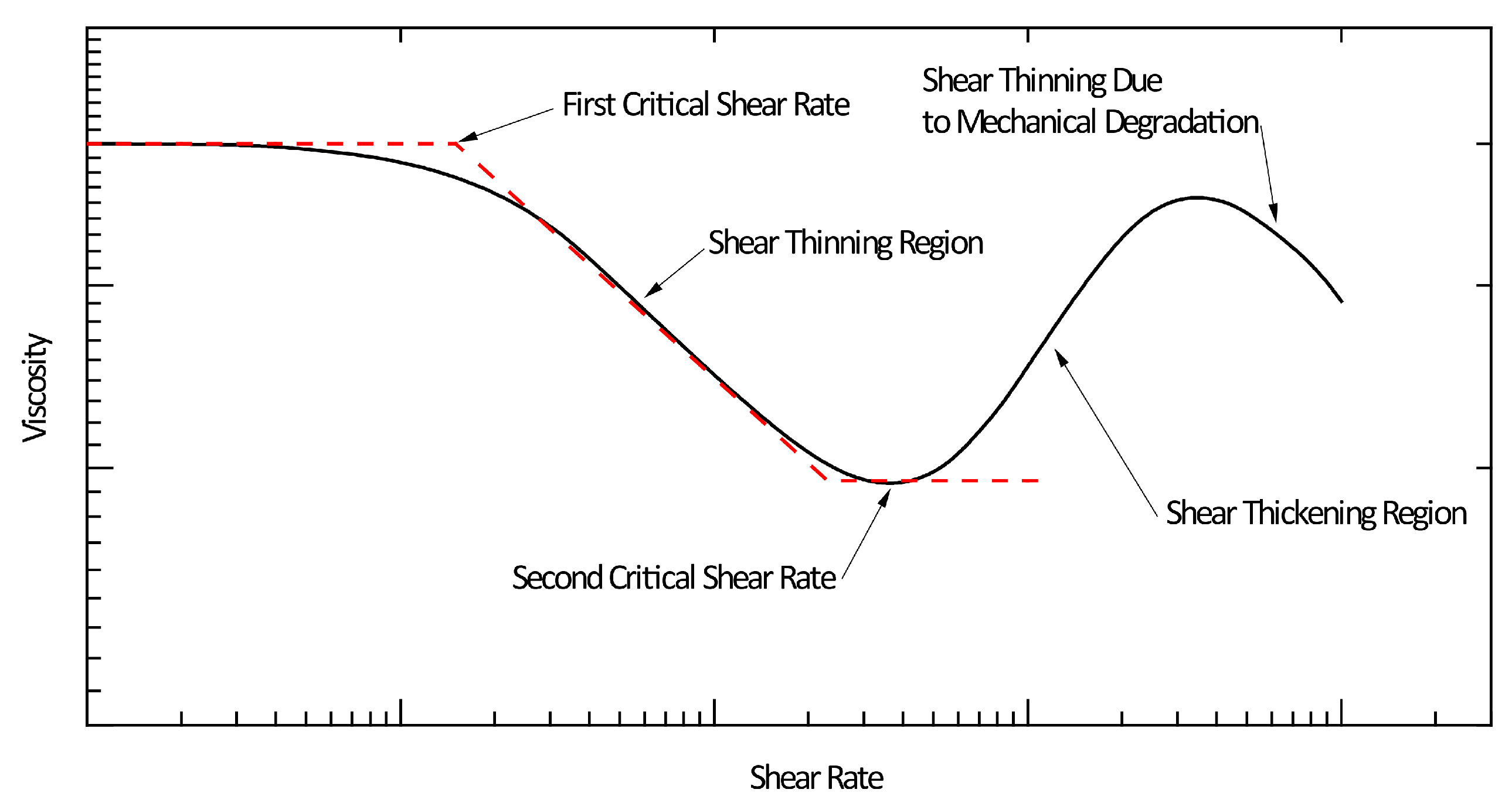
The viscoelastic behavior of polymer solutions in porous media is plotted in Figure 8. The three different regions of the UVM model can be distinguished. The fluid acts as a Newtonian fluid at very low shear rates. In between the first critical shear rate and second critical shear rate, the fluid behaves as a pseudoplastic fluid; the viscosity decreases as the shear rate does. Above the second critical shear rate, shear-thickening behavior can be observed.
Within polymer flooding, degradation of the polymers due to mechanical, chemical, thermal and biological mechanisms should be taken into account. Degradation of the polymer leads to a reduction in molecular weight and diminishes the thickening ability of the polymer. Polymer degradation is a function of time and is described by the following formula [45]:
where represents the molecular weight of the polymer, and is the degradation parameter.
3. Results
3.1. Introduction
The first results to be presented are the porosity and permeability fields created in COMSOL. Subsequently, the simulation is carried out in secondary recovery schemes and then the polymer EOR is analyzed. Moreover, an analysis of the meshing and the results obtained is presented in order to find the optimum element size. Subsequently, the particle tracing results and well efficiency are examined. Finally, the water flooding and polymer flooding are compared, after which a modification of the polymer flooding and its results are presented.
3.2. Porosity and Permeability
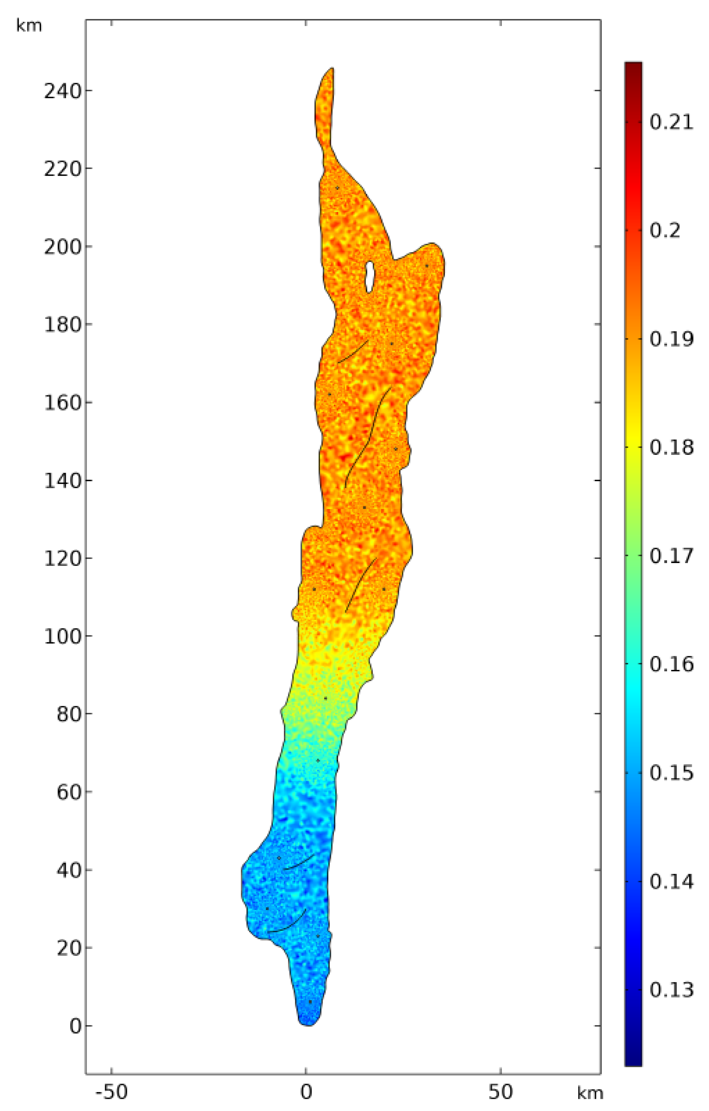
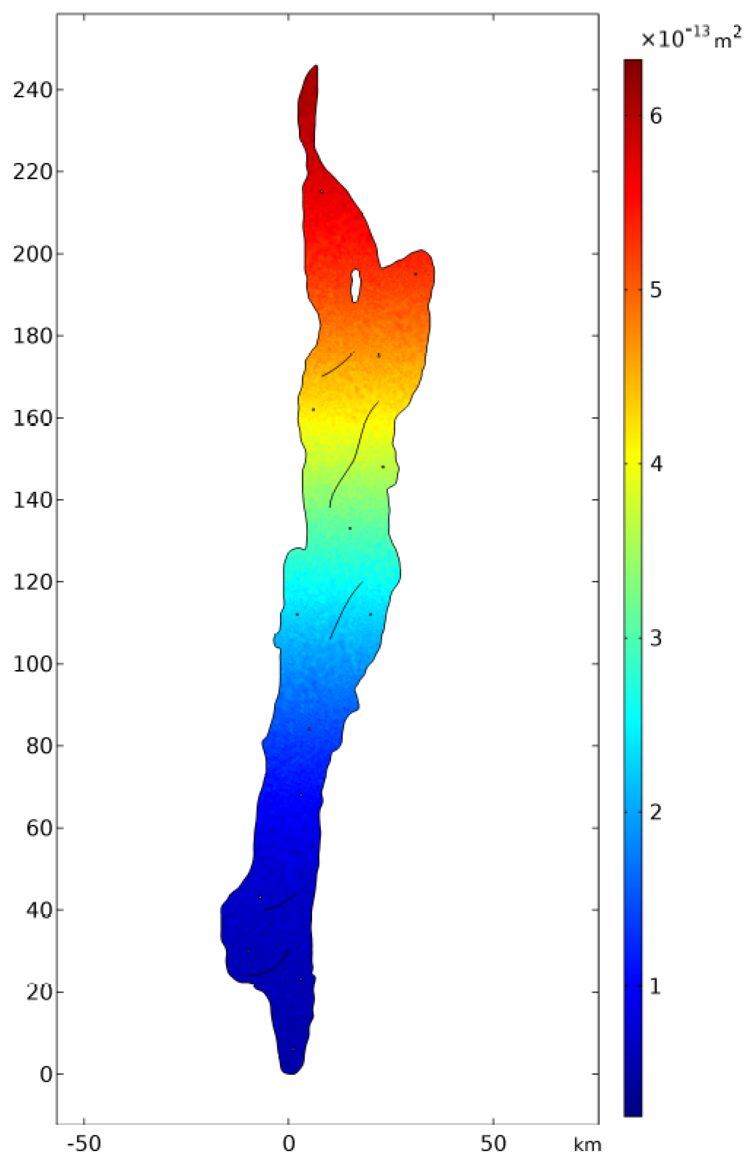
The porosity and permeability distribution, modeled in COMSOL, are illustrated in Figure 9 and Figure 10, respectively. The average porosity of the field is 0.179, and the average permeability is 291 mD. Both properties decrease from north to south and have an irregular distribution over the field as a result of the step and random functions used in COMSOL. It has been reported that the areas with low dolomite percentage are the areas with the lowest absolute permeabilities in the reservoir; therefore, considering Figure 6, we have set a number of thin, impermeable walls in these regions. For future research, it is deemed that these walls should allow a certain flow through them in order to match what actually happens in these areas [46,47].
3.3. Waterflooding
3.3.1. Meshing
The accuracy of the solution is related to the quality of the mesh, which is dependent on the number of elements. Therefore, it is important to study the outcomes of several meshes. This is achieved by studying the relative error and comparing the graphical results of the meshes. The fluid pressure drop in porous media is a reliable property for calculating the relative error. However, it should be mentioned that the total error of the simulation is not only in the pressure but also in other equations, such as the mass transfer equation. For estimating the relative error, the average fluid pressure drop is calculated by comparing the total pressure at the inlet and outlet [48,49]. The element properties of the different meshes and the corresponding relative error are given in Table 2.
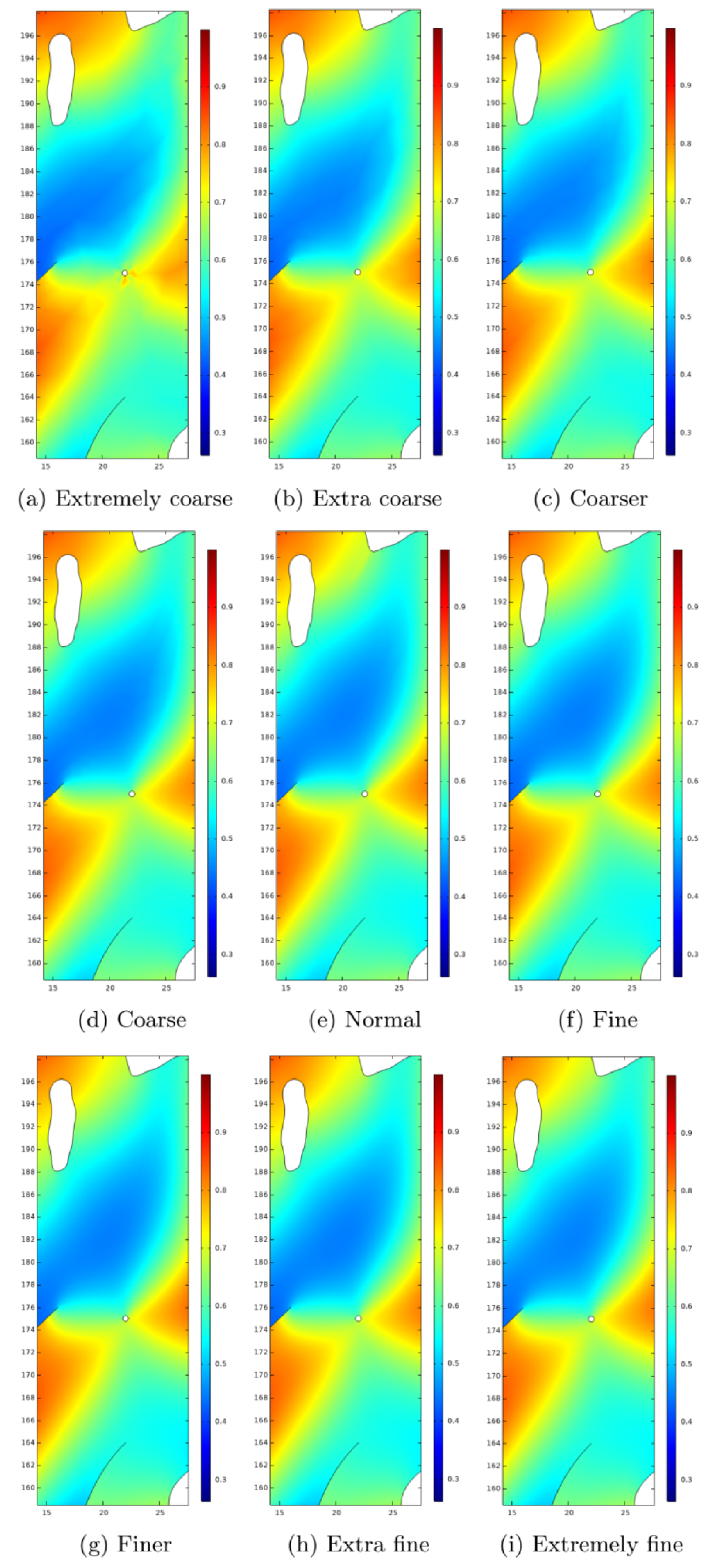
The error of all the mesh sizes is very low. From these results, it can be concluded that all the mesh sizes are suitable for the model. However, the graphical results are also relevant as these are used to visualize and study the flow and pressure in the oil field. Therefore, the graphical results of the saturation in the reservoir are compared in Figure 11.
The graphical comparison of the mesh sizes demonstrates no significant differences between the meshes. However, for the extremely coarse mesh, there is an irregularity at the producer well. Furthermore, the shape of the color distribution shows some deviations in the more coarse meshes, although these meshes had a small relative error. Based on this error and the graphical comparison, the finer mesh is selected. This mesh has an extremely small error and provides good graphical results. The mesh finer has significantly fewer elements compared to extremely fine, which reduces the computational calculations. In Figure 12, an overview and close-up of the mesh is given. The mesh is refined along the walls, wells and faults. This is necessary to obtain an accurate solution as the gradient of the calculated properties is large in these areas.
3.3.2. Shear Rate
Several formulas for the shear rate were found in the literature, as mentioned in Section 2.4. The shear rate values calculated by these formulas are given in Table 3, which shows that the values are all in the same range. The shear rate value of the most simple equation (indicated by number 1) has a value that is between the values of the other equations. Therefore, it was decided to use this formula for the calculation of the shear rate in the model.
3.3.3. Saturation
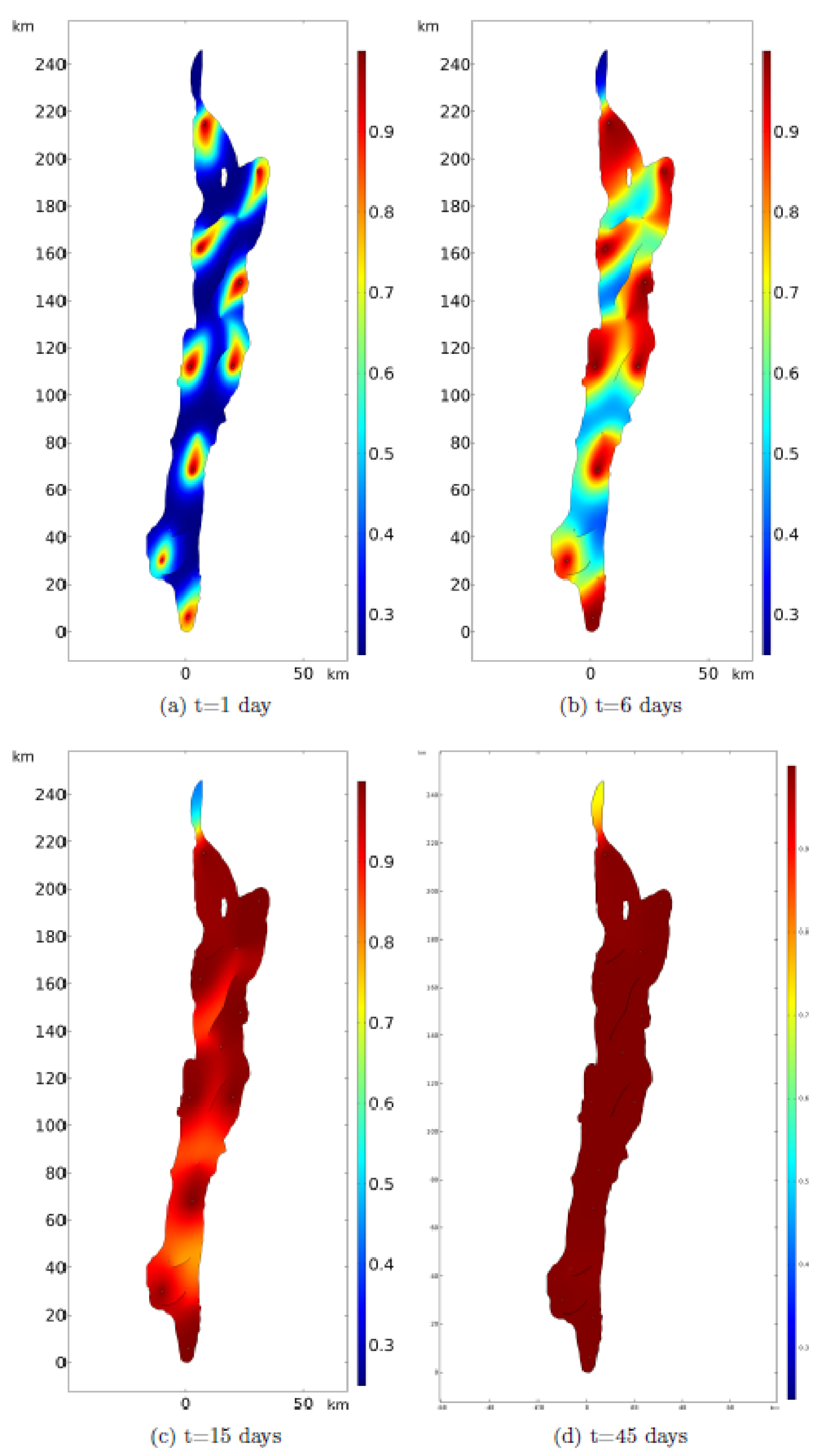
Figure 13 illustrates the normalized saturation within the Ghawar field as a function of time. The introduction of water to the field occurs at the injection wells, and the water saturation around these wells increases. Subsequently, the water migrates towards the producer wells, which is driven by the pressure gradient over the field. As the water inflow continues, the water saturation of the field keeps increasing. At days, the influence of the faults on the water distribution over the field is clearly visible. The faults are impermeable barriers, which makes it more difficult for the water to penetrate the areas around the faults, resulting in a lower saturation in these areas compared to the rest of the field. Furthermore, the water saturation is relatively low at the northern tip. This is a result of the narrow area through which water inflow and oil outflow have to occur simultaneously in order for water to penetrate this area.
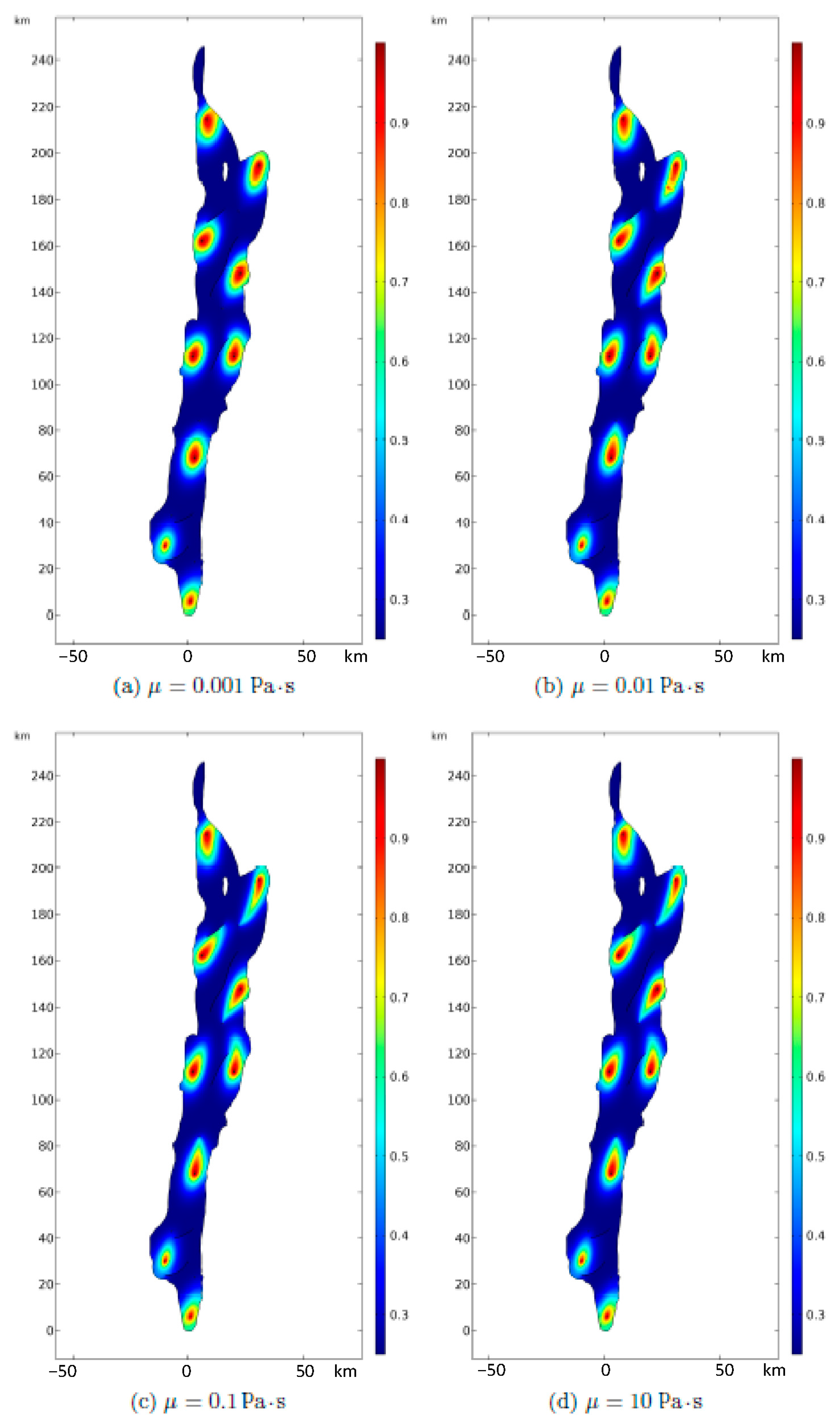
Though the oil properties throughout the field do not vary significantly, an extra study is carried out considering different oil viscosities. This also has a numerical purpose since the influence of the mobility ratio in the model’s behavior is well-known, and the goal was to test the model’s stability as well. The early water breakthrough for more viscous oils is clearly visible in Figure 14. For the low viscosity oil, the water propagates slower through the reservoir and forms a more stable front with the oil, which is illustrated by the rounder shape of the water saturation in figure (a) when the oil viscosity is similar to the water. However, this becomes more tapered with increasing oil viscosities, showing a sort of viscous fingering, which was not detected in the first case. Finally, it is worth mentioning that the saturation fields of the high viscosity oils are comparable, and no significant differences are appreciable.
3.4. Polymer Flooding
3.4.1. Saturation
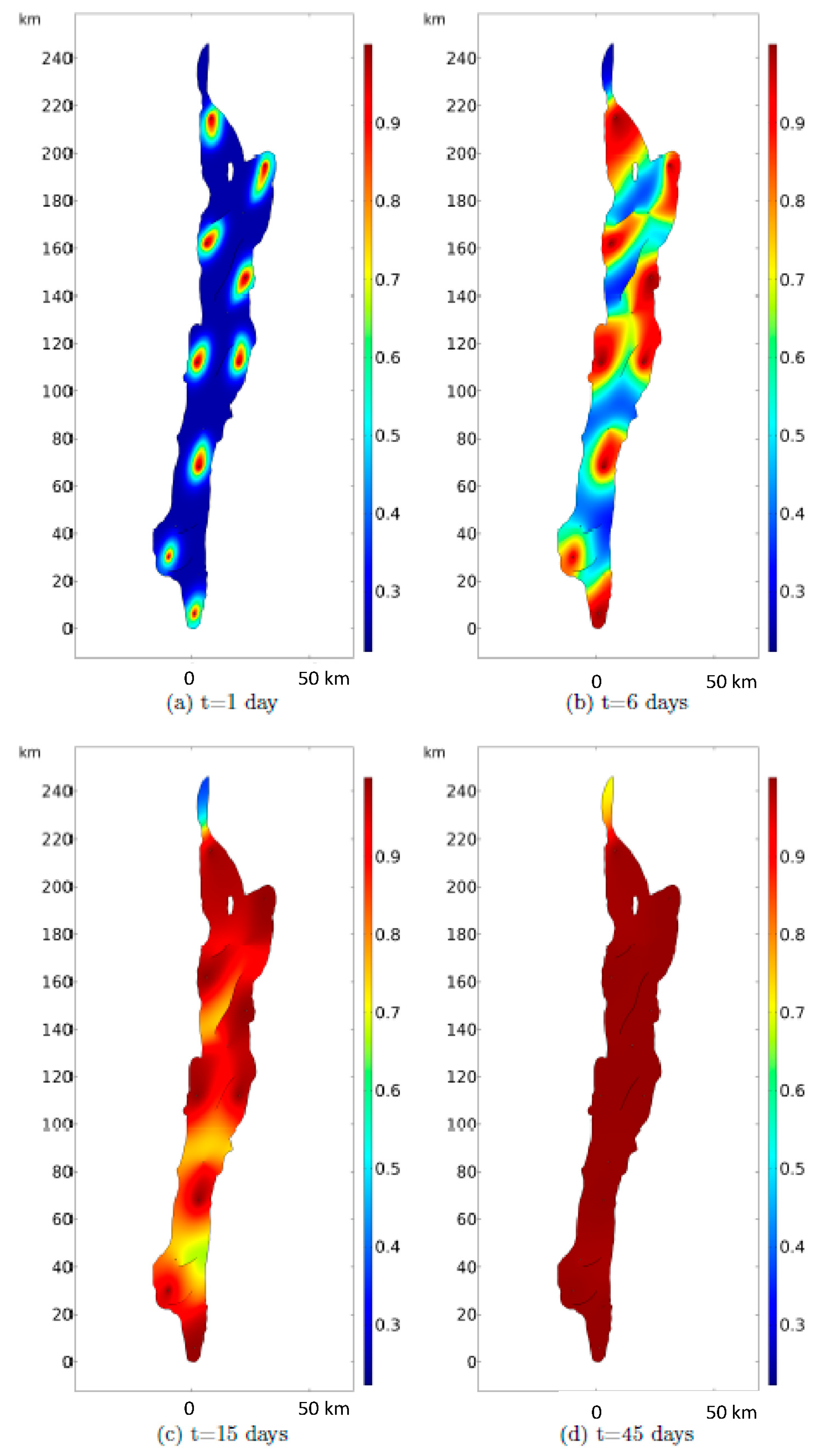
The normalized saturation of the Ghawar field for polymer flooding is illustrated in Figure 15. The graphical results demonstrate the same saturation distribution as for water flooding. It should be noted that the saturation in these results is the normalized saturation instead of the real saturation of the field. This will be further discussed in Section 3.5.
The viscosity of the polymer solution depends, among others, on the polymer’s molecular weight but also the architecture of the molecule (i.e., radius of gyration), and this also has a strong influence on the solution’s viscoelastic properties, which affect the recovery process. It is advised to consider in future models the influence of these parameters in the viscosity, since the polymer degradation primarily affects the molecular weight, and this modifies all of the other properties.
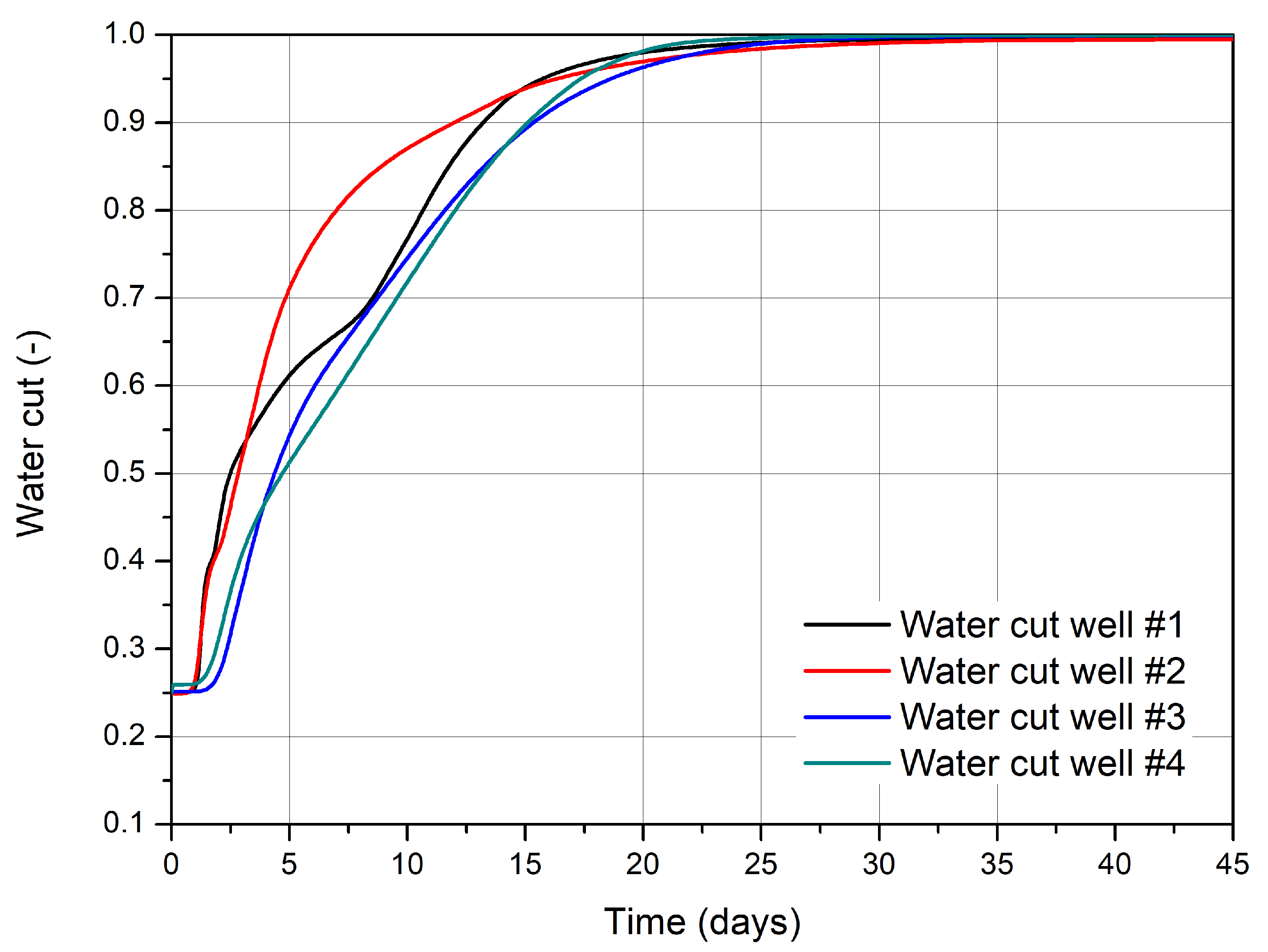
The water cuts for the producer wells during the polymer flooding are presented in Figure 16. Based on the results, all of the wells perform similarly in terms of water fraction produced, with the exception of well #2 (the second one from north to south); this well reaches higher values of water-cut during the first stages of the simulation, but after approximately 15 days, the values become similar to the other wells. The location and pattern might be further optimized in order to reach the water-cut economical threshold in all wells at the same time and in a shorter period of time.
3.4.2. Viscosity and Polymer Concentration
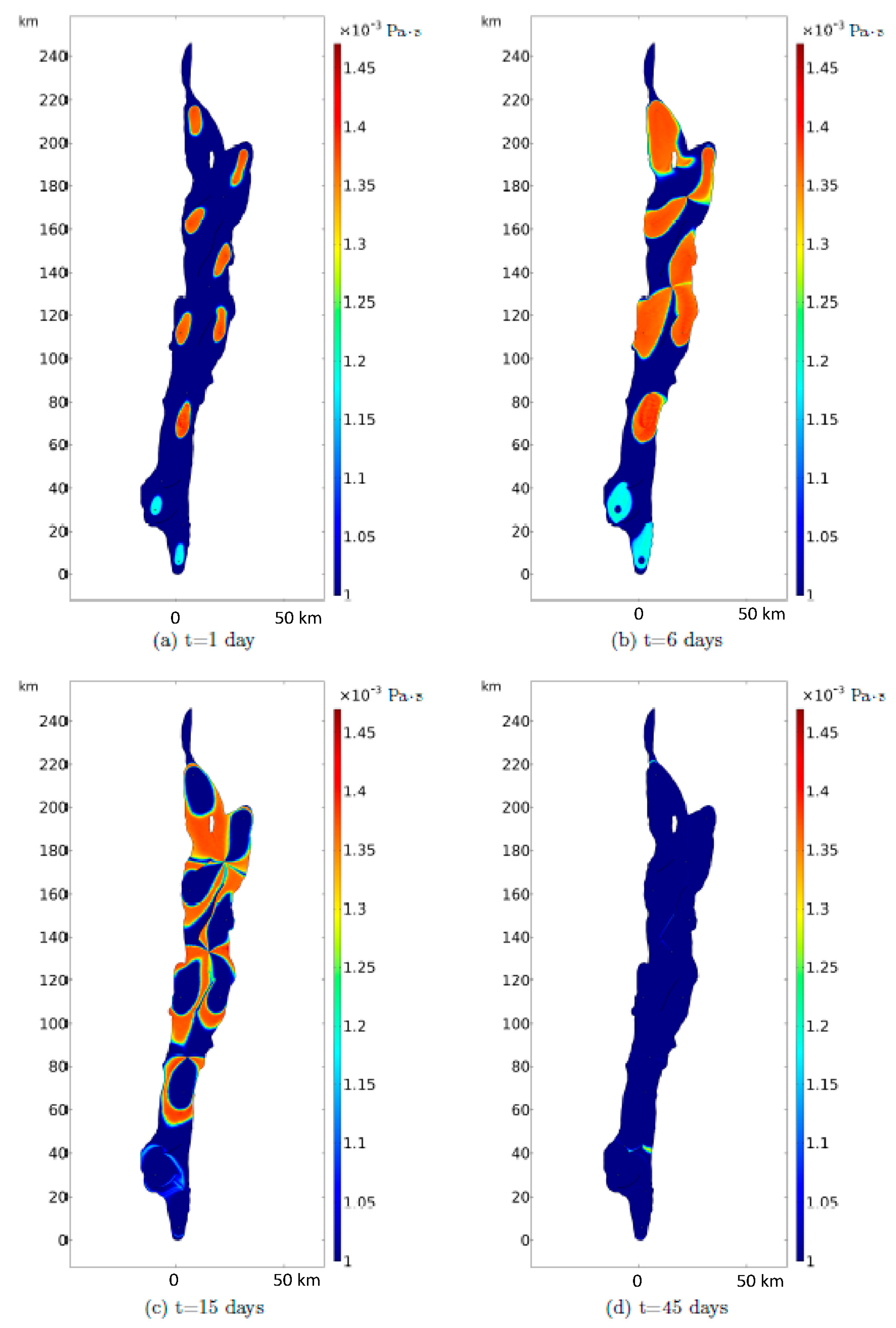
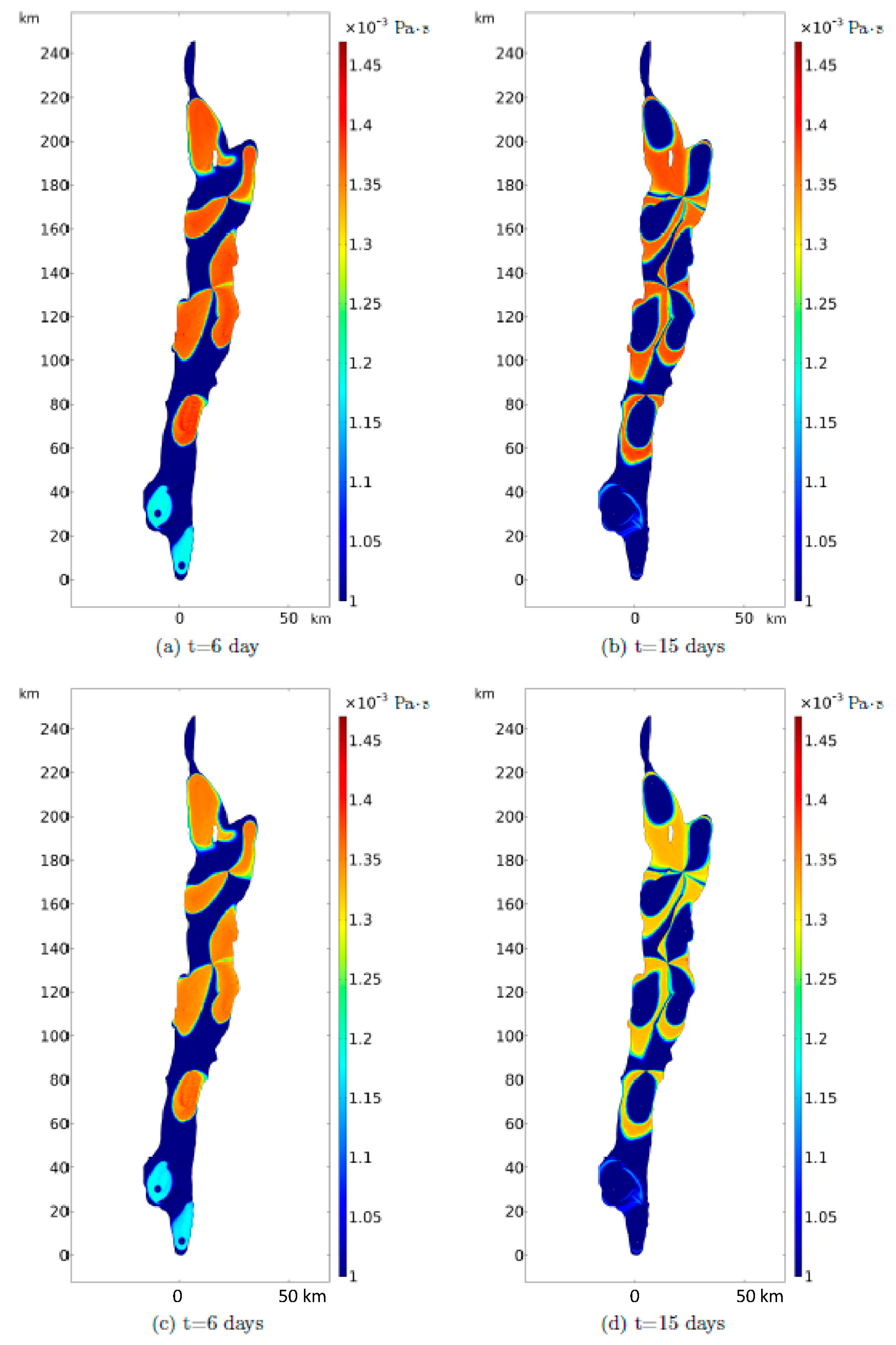
The viscosity is given in Figure 17. The figure confirms the strong relationship between the polymer concentration and the viscosity since this corresponds to the dependence of the viscosity on the polymer concentration. Two different polymer concentrations are injected in the field. At the northern part of the field, a polymer concentration of 10 mol/m is injected during the first 11.5 days. At the southern wells, a concentration of 4 mol/m is injected for a shorter period (5.8 days). The graphical results demonstrate that the polymer concentration results in a significant viscosity increase in the displacing fluid. Furthermore, it is clearly visible that the viscosity increase in the south of the field is lower compared to the north, which is a result of the different polymer concentrations injected. After injecting the polymer solutions, water flows in, which is illustrated by the low viscosity spots inside the higher viscosity ranges. As a remark, it is also evident that the increment in the viscosity, with respect to the water, is not as significant as in traditional polymer flooding processes, and higher viscosities should be simulated in further studies. The purpose of this paper is to create the model of Ghawar in COMSOL and to establish general guidelines for future EOR studies.
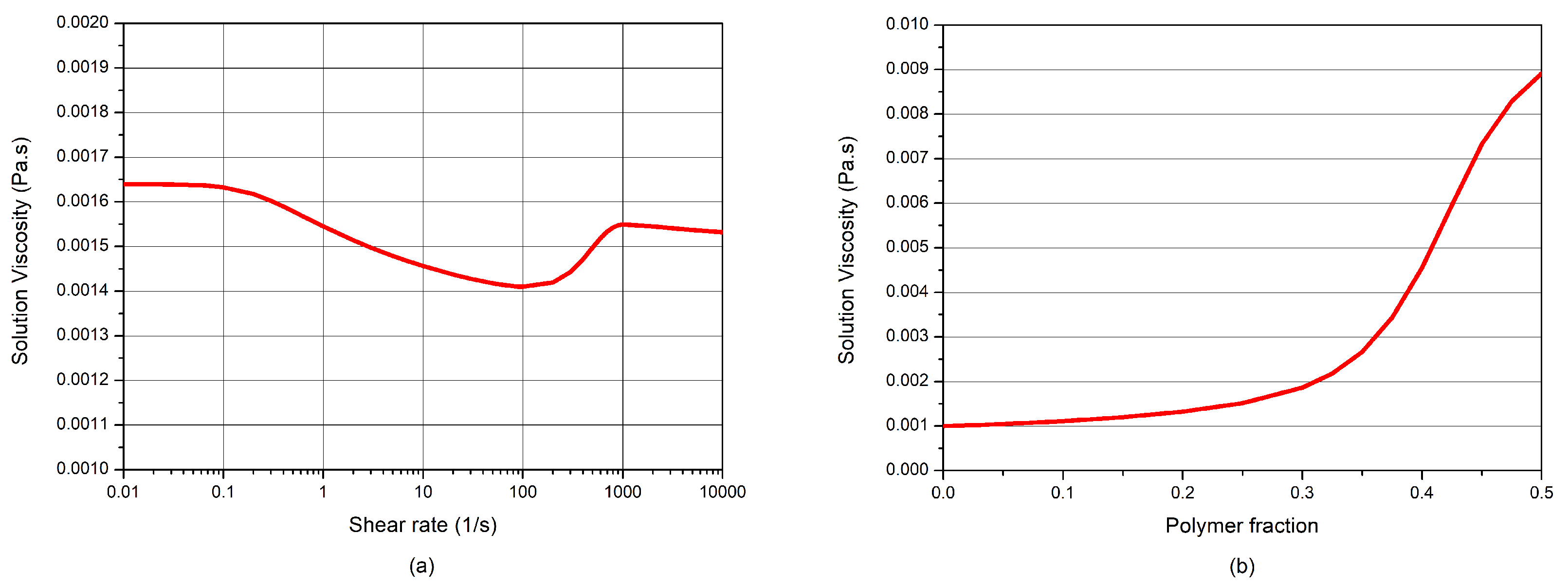
With respect to the last point, Figure 18 shows two plots of the polymer solution used in this paper: the left one is the polymer viscosity as a function of the shear rate, using the UVM model for a constant polymer volumetric concentration, and the right one is the polymer solution viscosity for the average shear rate found at the reservoir as a function of the polymer volumetric concentration. In the latter, we have limited the fraction due to operative conditions. In these plots, the polymer degradation is still not being considered, which will be studied in the next section. As mentioned in previous sections, the influence of the polymer in the viscosity is not noticeable in the operating conditions, though at higher concentrations, this becomes more noticeable. Nevertheless, the influence of the polymer on the viscosity is determined by a number of constants, which must be measured carefully before any simulation is carried out.
3.4.3. Polymer Degradation
Polymer degradation reduces the polymer concentration in the field, and it is a function of time. The degradation rate determines the speed of decrease in the polymer concentration. Within this section, the influence of polymer degradation on the viscosity of the displacing fluid is studied. Figure 19 illustrates the decrease in viscosity as a result of this degradation. The polymer solution viscosity with degradation compared to the polymer solution viscosity without is significantly reduced. Furthermore, it is demonstrated that the polymer concentration reduces further over time, which is indicated by the larger reduction in viscosity for 15 days compared to the viscosity of 6 days.
3.4.4. Particle Tracing
Particle tracing is a theoretical study performed to analyze the residence time and retention of virtual particles in the field. This study of retention is two-fold: to study the flow and/or entrapment of polymers, not because of mechanical entrapment, but because of the general well location design; secondly, to link this with future studies involving nanoparticles. It is deemed of the utmost importance to understand the percentage of retention and the places in order to avoid possible (environmental) problems. In total, 6500 particles were injected into the field, from which 1500 particles were injected at the two southern injection wells and the other 5000 particles at the remaining injection wells. From these particles, 6480 were recovered at the producer wells, which indicates that only 0.3% of these particles will be retained in the reservoir after polymer flooding. This does not indicate that the polymer retention will be low, but the fact that the positioning of the wells in the field has been performed properly.
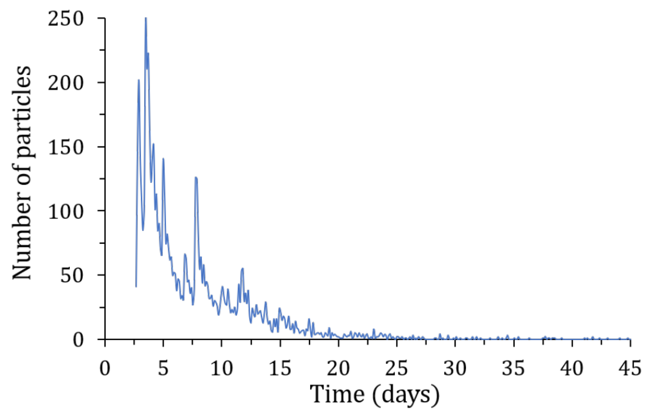
Furthermore, the average residence time of the particles in the reservoir is studied, which is illustrated in Figure 20. The average residence time of the particles in the field was 7.54 days and the graph demonstrates that most particles (76%) were recovered within the first 10 days. A short residence time of the polymer is favorable to reduce the degradation of the polymer in the reservoir.
3.4.5. Well Efficiency
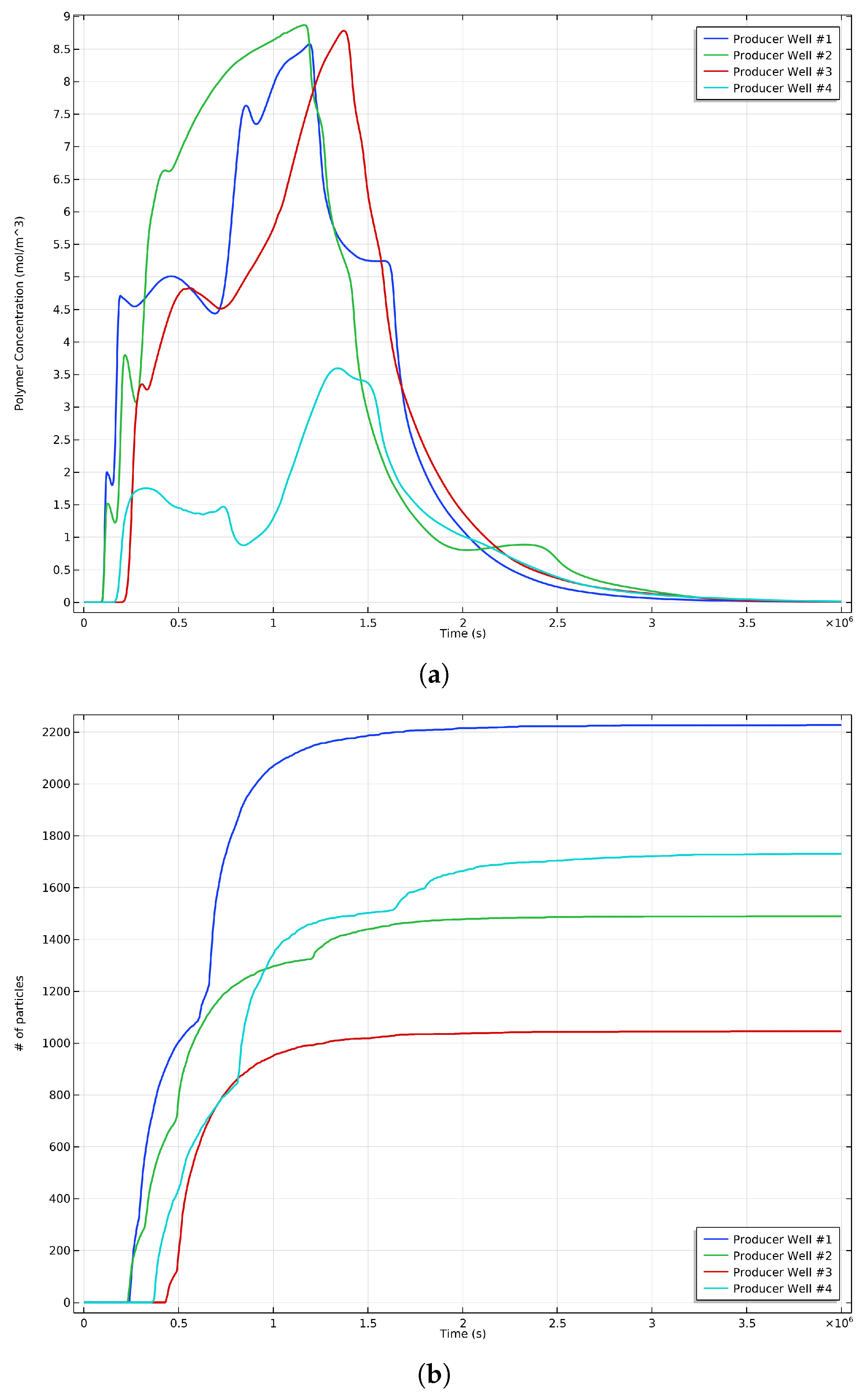
To investigate the efficiency of the wells, the polymer concentration and number of particles at the wells are evaluated. The particles are injected into the field at . It can be seen that most particles are recovered within the first stage of oil recovery. The producers are numbered from north to south, and the results are illustrated in Figure 21. From these graphs, it is shown that the particles injected at producer wells near walls have a longer retention time compared to the particles injected in the north. This is in accordance with the figures of the saturation, which demonstrate that the displacing fluid injected at these wells reaches the producers at a later stage. Furthermore, these particles have a lower efficiency, which is mainly due to the lower number of particles injected in the southern area. The polymer concentration demonstrates that all producer wells have relatively high efficiency. The results from the particle tracing imply a relatively low efficiency for producer well number two. However, the polymer concentration graph demonstrates a second peak for producer well number two. The second peak is due to the displacing fluid moving around the fault near producer well number two. The same peak is observed for producer well number three, which is also related to the faults around this well.
3.5. Modified Polymer Flooding
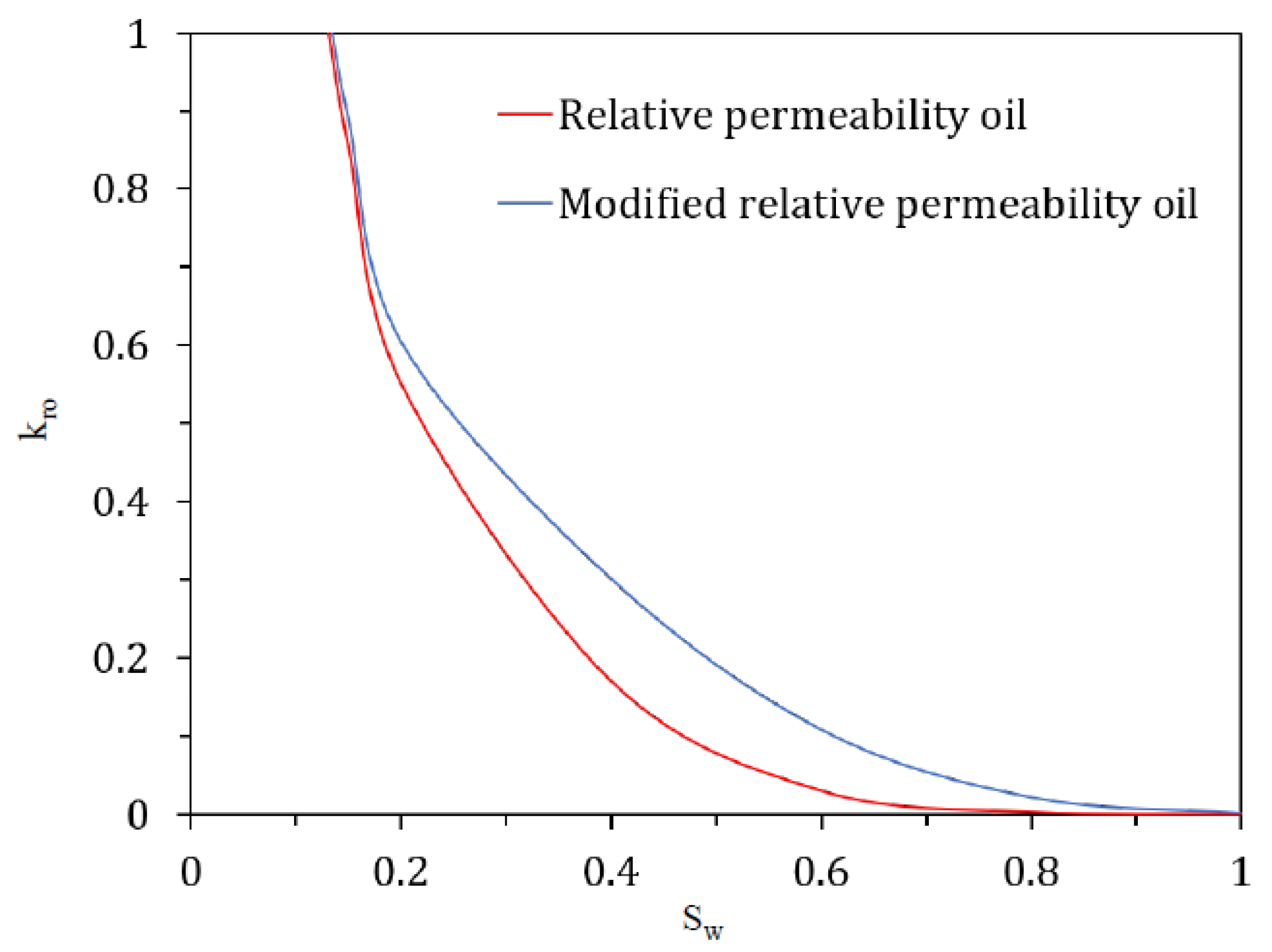
The polymer concentration does not influence the relative permeability of oil () in COMSOL. However, is a function of the polymer concentration and increases for higher polymer concentrations. Therefore, a modification for the relative permeability is proposed, which is demonstrated by Equation (24). The new is a function of the original relative permeability (), water saturation () and polymer concentration (). The new curve for the relative permeability is illustrated in Figure 21, and it tends to reproduce the slight variations in the relative oil permeability reported by several authors [44,50,51].
There is still a dispute in the scientific world whether polymers can actually decrease the residual oil saturation or not. While several authors have presented evidence that polymer flooding only affects the macroscopic efficiency via the increase in the viscosity, other authors have reported the decrease in the residual saturation by means of, for instance, the viscoelastic effects [10,16,18,36,45]. In this paper, it is considered the last point of view, that is, that the polymer actually affects both the macro- and the microscopic efficiencies, decreasing under certain injection conditions the residual oil saturation (Figure 22).
The proposed modification slightly affects the effective normalized saturation of the field (Figure 7 and Figure 23). However, it has a major influence on the real oil saturation of the field since the residual oil saturation is modified () due to the presence of the polymer in the aqueous phase. To calculate the residual oil saturation, the following equations are used:
where A, B and C are fitting parameters. Equation (26) represents the standard oil permeability curve without the polymer (Figure 22—dashed line; Figure 23—red line). This curve is affected then by the polymer concentration, using Equation (24) (Figure 23—black line). However, this dependency renders a non-linear problem since the Darcy equations used to calculate velocity and pressure fields depend on the relative oil permeability. Then, the problem must be solved numerically using an iterative approach per timestep.
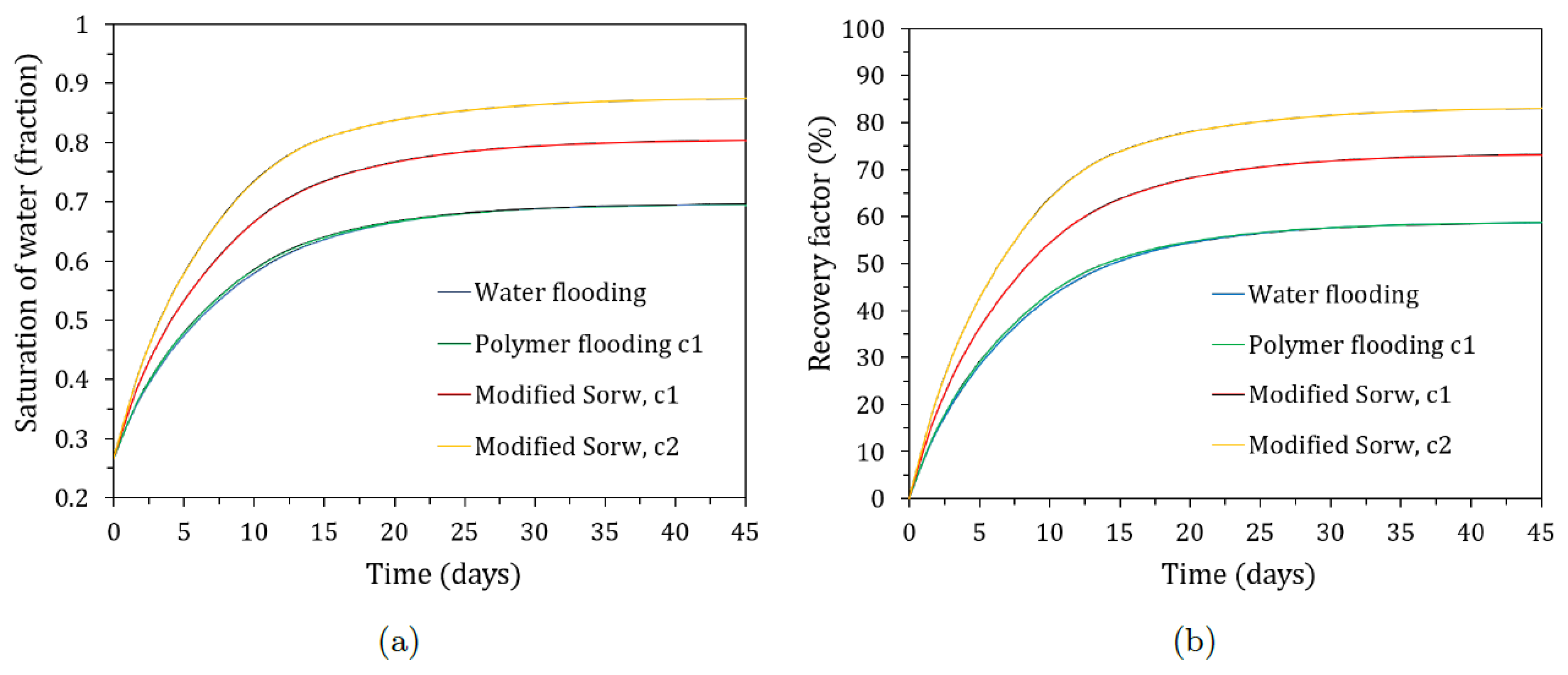
In Figure 24, the result of polymer flooding with the modified equation is compared to the results of water flooding and the original polymer flooding. For calculating the saturation of the modified polymer flooding, the average value of is used due to the following: when the polymer concentration increases, the value of decreases and the saturation is increased, whereas when the polymer concentration is decreased, the value of also increases, which leads to a reduction in saturation. However, it is impossible for the water saturation to decrease as oil is only flowing out of the reservoir. Therefore, to estimate the saturation, the average value is used. However, in reality, the slope of the curve for the modified polymer flooding is steeper at the beginning and flattens earlier than the curve demonstrated in Figure 24. Nevertheless, the graph shows a significant difference in the recovery factor between water flooding and polymer flooding. Furthermore, it is demonstrated that the concentration of the polymer has a significant influence on the oil recovery; a lower concentration of polymer renders a lower recovery factor.
4. Conclusions
An advanced, novel numerical model is developed to study oil recovery within the Ghawar field. First, the geometry and porosity and permeability field of the Ghawar field were successfully modeled in COMSOL Multiphysics. In addition, the momentum and mass transfer equations of the model were successfully coupled within one study, which resulted in mutual dependency. Several studies were performed, and the results were analyzed in the present paper, with the following conclusions:
- Waterflooding of the Ghawar field resulted in a recovery factor of 58%, which is in line with the literature values considering some ideal properties used in the model, for example, the temperature of the reservoir. However, there was no significant difference between the recovery factors of water flooding and polymer flooding. This is also due to the fact that the polymer’s influence on the viscosity is not significant enough to improve the macroscopic recovery efficiency.
- The relatively low recovery factor for polymer flooding was caused by the way in which the oil relative permeability was modeled. The oil relative permeability was independent of the polymer concentration, which resulted in the same residual oil saturation for polymer flooding as for waterflooding. Modification of the equation resulted in a significant increase in recovery factor by approximately 15–25% compared to water flooding, depending on the polymer concentration.
- The influence of oil viscosity on the recovery factor for both waterflooding and polymer flooding was examined. It could be concluded that a lower mobility ratio between the oil and water results in a higher recovery efficiency.
- In addition, particle trajectories in the reservoir were studied to investigate the influence of polymer retention and the residence time of polymers in the reservoir. The particle tracing evaluation indicates that a very small percentage of the polymer is retained in the reservoir, which is favorable since the retention of polymers in the reservoir may have a negative influence on the environment, depending on the polymer used.
- This last point allowed us to study polymer recycling, which could possibly reduce the costs of enhanced oil recovery; so far, this has proven too hard or impossible to perform due to the complexity of the fluids produced, but it is deemed that this should be investigated in further studies. The results showed that 76% of the polymer was recovered within 10 days. The residence time is of importance for the stability of the polymers; longer residence times require more stable polymers. Furthermore, degradation of the polymer in the reservoir as a result of long residence times may increase the cost of EOR projects.
- A well analysis was performed, which involves the efficiency of the wells. Within the model, it was chosen to surround one producer well with several injection wells—14 wells in total, including 9 injection and 5 producer wells. The concentration of polymers at the wells and the number of particles therein were examined. From this evaluation, it could be concluded that the well placement was performed properly since the efficiency of all the wells was remarkably high. This study was not meant to optimize the retention time but to explore whether different wells had different timescales. Had the output shown that one of the wells had a different production profile, then the location would have needed to be rearranged.
Author Contributions
Methodology; software; validation; formal analysis; investigation; writing—original draft preparation, M.B.; project administration, F.P.; conceptualization; resources; writing—review and editing; visualization; supervision, P.D. All authors have read and agreed to the published version of the manuscript.
Funding
This research received no external funding.
Data Availability Statement
Not applicable.
Conflicts of Interest
The authors declare no conflict of interest.
Abbreviations
The following abbreviations are used in this manuscript:
| EOR | Enhanced Oil Recovery |
| HPAM | Hydrolyzed Polyacrylamide |
| OOIP | Original Oil in Place |
| UVM | Unified Viscosity Model |
| Nomenclature | |
| C | Concentration |
| Diffusion tensor | |
| Molecular diffusion [m/s] | |
| Longitudinal dispersion [m/s] | |
| Transversal dispersion [m/s] | |
| d | Depth [m] |
| F | Force [N] |
| g | Acceleration of gravity [m/s] |
| K | Absolute Permeability [mD]/[m] |
| Boltzmann’s constant [J/K] | |
| Relative Permeability | |
| Molecular weight [Da] | |
| n | Power law exponent |
| UVM parameter | |
| p | Pressure [Pa] |
| Bottomhole pressure [Pa] | |
| Particle radius [m] | |
| Well radius [m] | |
| S | Saturation |
| T | Temperature [K] |
| t | Time [s] |
| u | Darcy velocity [m/s] |
| V | Volume [m] |
| v | Velocity [m/s] |
| Greek Letters | |
| Shear rate [1/s] | |
| Domain Boundary | |
| UVM parameter | |
| Phase viscosity [mPa · s] | |
| Formation Porosity | |
| Density [kg/m] | |
| Elastic viscosity (shear thickening) | |
| Elastic viscosity (shear thinning) | |
| Reservoir Domain | |
| Superscripts | |
| j | Phase |
| o | Oleus phase |
| w | Water Phase |
| Subscripts | |
| c | Capillary |
| Shear-thickening | |
| External | |
| i | Component |
| Injection | |
| Irreducible | |
| Non-wetting phase | |
| o | Petroleum component |
| p | Polymer component |
| r | Residual |
| s | Surface |
| Shear-thinning | |
| t | Total |
| w | Water component |
References
- Maugeri, L. Oil: The Next Revolution Discussion Paper; Belfer Center for Science and International Affairs: Cambridge, MA, USA, 2012; pp. 142–149. [Google Scholar]
- Murray, T.J. Dr Abraham Gesner: The father of the petroleum industry. J. R. Soc. Med. 1993, 86, 43–44. [Google Scholar] [PubMed]
- OECD/IEA. World Energy Outlook; WEO 2008; IEA Publishing: Paris, France, 2008. [Google Scholar]
- Atwater, G.I.; McLeroy, P.G.; Riva, J.P. Petroleum. Available online: https://www.britannica.com/science/petroleum (accessed on 25 May 2022).
- Druetta, P.; Raffa, P.; Picchioni, F. Chemical enhanced oil recovery and the role of chemical product design. Appl. Energy 2019, 252, 113480. [Google Scholar] [CrossRef]
- Druetta, P.; Picchioni, F. Branched polymers and nanoparticles flooding as separate processes for enhanced oil recovery. Fuel 2019, 257, 115996. [Google Scholar] [CrossRef]
- Satter, A.; Iqbal, G.M.; Buchwalter, J.L. Practical Enhanced Reservoir Engineering; PennWell Books: Tulsa, OK, USA, 2008. [Google Scholar]
- Harris, P.M.; Weber, L.J. Giant Hydrocarbon Reservoirs of the World: From Rocks to Reservoir Characterization and Modeling; AAPG Memoir 88; American Association of Petroleum Geologists: Tulsa, OK, USA, 2006. [Google Scholar]
- Zendehboudi, S.; Bahadori, A. Shale Oil and Gas Handbook: Theory, Technologies, and Challenges; Elsevier Science: Amsterdam, The Netherlands, 2016. [Google Scholar]
- Muggeridge, A.; Cockin, A.; Webb, K.; Frampton, H.; Collins, I.; Moulds, T.; Salino, P. Recovery rates, enhanced oil recovery and technological limits. Philos. Trans. R. Soc. A Math. Phys. Eng. Sci. 2014, 372, 20120320. [Google Scholar] [CrossRef] [Green Version]
- Ahmed, T. Reservoir Engineering Handbook; Gulf Publishing Company: Houston, TX, USA, 2000. [Google Scholar]
- Shepherd, M. Oil Field Production Geology; American Association of Petroleum Geologists: Tulsa, OK, USA, 2009. [Google Scholar]
- Al-Wahaibi, Y.; Al-Hashmi, A.; Joshi, S.; Mosavat, N.; Rudyk, S.; Al-Khamisi, S.; Al-Kharusi, T.; Al-Sulaimani, H. Mechanistic study of surfactant/polymer adsorption and its effect on surface morphology and wettability. In Proceedings of the SPE Oil and Gas India Conference and Exhibition, Mumbai, India, 4–6 April 2017. [Google Scholar]
- BP. Statistical Review of World Energy June 2014; Annual Report 63, BP p.l.c.; BP Group: London, UK, 2014. [Google Scholar]
- Kamal, M.S.; Sultan, A.S.; Al-Mubaiyedh, U.; Hussein, I.A. Review on polymer flooding: Rheology, adsorption, stability, and field applications of various polymer systems. Polym. Rev. 2015, 55, 491–530. [Google Scholar] [CrossRef]
- Lake, L.W. Enhanced Oil Recovery; Prentice-Hall Inc.: Englewood Cliffs, NJ, USA, 1989. [Google Scholar]
- Alvarado, V.; Manrique, E. Enhanced oil recovery: An update review. Energies 2010, 3, 1529–1575. [Google Scholar] [CrossRef]
- Zhang, Z.; Li, J.; Zhou, J. Microscopic roles of “viscoelasticity” in HPMA polymer flooding for EOR. Transp. Porous Media 2011, 86, 229–244. [Google Scholar] [CrossRef] [Green Version]
- Sorkhabi, R. The king of giant fields. GeoExPro 2010, 7, 24–29. [Google Scholar]
- Phelps, R.; Strauss, J. Simulation of vertical fractures and stratiform permeability of the Ghawar field. In Proceedings of the SPE Reservoir Simulation Symposium, Houston, TX, USA, 11–14 February 2001. [Google Scholar]
- Al-Shuhail, A.; Alshuhail, A.; Khulief, Y.; Salam, S.; Chan, S.; Ashadi, A.; Al-Lehyani, A.; Almubarak, A.; Khan, M.; Khan, S.; et al. KFUPM Ghawar digital viscoelastic seismic model. Arab. J. Geosci. 2019, 12, 245. [Google Scholar] [CrossRef]
- Al-Anazi, B.D. What you know about the Ghawar oil field, Saudi Arabia? CSEG Rec. 2007, 32, 40–43. [Google Scholar]
- Ameen, M.S.; Smart, B.G.; Somerville, J.M.; Hammilton, S.; Naji, N.A. Predicting rock mechanical properties of carbonates from wireline logs (a case study: Arab-D reservoir, Ghawar field, Saudi Arabia). Mar. Pet. Geol. 2009, 26, 430–444. [Google Scholar] [CrossRef]
- Cantrell, D.; Swart, P.; Hagerty, R. Genesis and characterization of dolomite, Arab-D reservoir, Ghawar field, Saudi Arabia. GeoArabia 2004, 9, 11–36. [Google Scholar] [CrossRef]
- Druetta, P.; Tesi, P.; Persis, C.D.; Picchioni, F. Methods in Oil Recovery Processes and Reservoir Simulation. Adv. Chem. Eng. Sci. 2016, 6, 39. [Google Scholar] [CrossRef] [Green Version]
- Saner, S.; Al-Hinai, K.; Perincek, D. Surface expressions of the Ghawar structure, Saudi Arabia. Mar. Pet. Geol. 2005, 22, 657–670. [Google Scholar] [CrossRef]
- Al-Dhafeeri, A.M. High-Permeability Carbonate Zones (Super-K) in Ghawar Field (Saudi Arabia), Identified, Characterized, and Treated by Gels; New Mexico Institute of Mining and Technology: Socorro, NM, USA, 2004. [Google Scholar]
- Gerlich, V.; Sulovská, K.; Zálesák, M. COMSOL multiphysics validation as simulation software for heat transfer calculation in buildings: Building simulation software validation. Measurement 2013, 46, 2003–2012. [Google Scholar] [CrossRef] [Green Version]
- Alioua, T.; Agoudjil, B.; Boudenne, A. Numerical study of heat and moisture transfers for validation on bio-based building materials and walls. In Proceedings of the International Conference on Numerical Modelling in Engineering, Ghent, Belgium, 28–29 August 2018; Springer: Berlin/Heidelberg, Germany, 2018; pp. 81–89. [Google Scholar]
- Lindsay, R.; Catrell, D.; Hughes, G.; Keith, T.; Mueller, H.; Russell, S. Ghawar Arab-D reservoir: Widespread porosity in shoaling-upward carbonate cycles, Saudi Arabia. In Giant hydrocarbon Reservoirs of the World: From Rocks to Reservoir Characterization and Modelling; AAPG Memoir 88; AAPG: Tulsa, OK, USA, 2006; pp. 97–137. [Google Scholar]
- Bear, J. Dynamics of Fluids in Porous Media; American Elsevier Publishing Company: New York, NY, USA, 1972. [Google Scholar]
- Chen, Z.; Huan, G.; Ma, Y. Computational Methods for Multiphase Flows in Porous Media; Society for Industrial and Applied Mathematics: Philadelphia, PA, USA, 2006. [Google Scholar]
- Kuzmin, D. A Guide to Numerical Methods for Transport Equations; University Erlangen-Nuremberg: Erlangen, Germany, 2010. [Google Scholar]
- Gerritsen, M.; Durlofsky, L. Modeling fluid flow in oil reservoirs. Annu. Rev. Fluid Mech. 2005, 37, 211–238. [Google Scholar] [CrossRef]
- Wegner, J.; Ganzer, L. Numerical simulation of oil recovery by polymer injection using COMSOL. In Proceedings of the 2012 COMSOL Conference, Milan, Italy, 10–12 October 2012. [Google Scholar]
- Sheng, J. Enhanced Oil Recovery Field Case Studies; Gulf Professional Publishing: Waltham, MA, USA, 2013. [Google Scholar]
- Maia, A.; Villetti, M.A.; Vidal, R.R.; Borsali, R.; Balaban, R.C. Solution properties of a hydrophobically associating polyacrylamide and its polyelectrolyte derivatives determined by light scattering, small angle X-ray scattering and viscometry. J. Braz. Chem. Soc. 2011, 22, 489–500. [Google Scholar] [CrossRef] [Green Version]
- Sotiropoulos, K.; Papagiannopoulos, A. Modification of xanthan solution properties by the cationic surfactant DTMAB. Int. J. Biol. Macromol. 2017, 105, 1213–1219. [Google Scholar] [CrossRef]
- Matyka, M.; Khalili, A.; Koza, Z. Tortuosity-porosity relation in porous media flow. Phys. Rev. E 2008, 78, 026306. [Google Scholar] [CrossRef] [Green Version]
- Ghanbarian, B.; Hunt, A.G.; Ewing, R.P.; Sahimi, M. Tortuosity in porous media: A critical review. Soil Sci. Soc. Am. J. 2013, 77, 1461–1477. [Google Scholar] [CrossRef]
- Carman, P. Fluid flow through granular beds. Chem. Eng. Res. Des. 1997, 75, S32–S48. [Google Scholar] [CrossRef]
- Delshad, M.; Kim, D.H.; Magbagbeola, O.A.; Huh, C.; Pope, G.A.; Tarahhom, F. Mechanistic interpretation and utilization of viscoelastic behavior of polymer solutions for improved polymer-flood efficiency. In Proceedings of the SPE Symposium on Improved Oil Recovery, Tulsa, OK, USA, 24–28 April 2008. [Google Scholar]
- Druetta, P.; Picchioni, F. Surfactant-polymer interactions in a combined enhanced oil recovery flooding. Energies 2020, 13, 6520. [Google Scholar] [CrossRef]
- Jiang, W.; Hou, Z.; Wu, X.; Song, K.; Yang, E.; Huang, B.; Dong, C.; Lu, S.; Sun, L.; Gai, J.; et al. A new method for calculating the relative permeability curve of polymer flooding based on the viscosity variation law of polymer transporting in porous media. Molecules 2022, 27, 3958. [Google Scholar] [CrossRef] [PubMed]
- Druetta, P.; Picchioni, F. Influence of the polymer degradation on enhanced oil recovery processes. Appl. Math. Model. 2019, 69, 142–163. [Google Scholar] [CrossRef]
- Cantrell, D.; Swart, P.; Handford, R.; Kendall, C.G.; Westphal, H. Geology and production significance of Dolomite, Arab-D reservoir, Ghawar field, Saudi Arabia. GeoArabia 2001, 6, 45–60. [Google Scholar] [CrossRef]
- Lucia, F.; Jennings, J.; Rahnis, M.; Meyer, F. Permeability and rock fabric from wireline logs, Arab-D reservoir, Ghawar field, Saudi Arabia. GeoArabia 2001, 6, 619–646. [Google Scholar] [CrossRef]
- Gharibshahi, R.; Jafari, A.; Haghtalab, A.; Karambeigi, M.S. Application of CFD to evaluate the pore morphology effect on nanofluid flooding for enhanced oil recovery. RSC Adv. 2015, 5, 28938–28949. [Google Scholar] [CrossRef]
- Rostami, P.; Sharifi, M.; Aminshahidy, B.; Fahimpour, J. The effect of nanoparticles on wettability alteration for enhanced oil recovery: Micromodel experimental studies and CFD simulation. Pet. Sci. 2019, 16, 859–873. [Google Scholar] [CrossRef] [Green Version]
- Wang, Q.; Liu, X.; Meng, L.; Jiang, R.; Fan, H. The numerical simulation study of the oil-water seepage behavior dependent on the polymer concentration in polymer flooding. Energies 2020, 13, 5125. [Google Scholar] [CrossRef]
- Zhong, H.; Zhang, W.; Fu, J.; Lu, J.; Yin, H. The performance of polymer flooding in heterogeneous type II reservoirs—An experimental and field investigation. Energies 2017, 10, 454. [Google Scholar] [CrossRef] [Green Version]
Figure 1.
Scheme showing the oil recovery stages and the different techniques employed in EOR (reprinted/adapted with permission from [5]).
Figure 1.
Scheme showing the oil recovery stages and the different techniques employed in EOR (reprinted/adapted with permission from [5]).

Figure 2.
Geographical location of the Ghawar oil field. In the image, the Jurassic oilfields are depicted in green and the gas fields in red (reprinted/adapted with permission from [26]).
Figure 2.
Geographical location of the Ghawar oil field. In the image, the Jurassic oilfields are depicted in green and the gas fields in red (reprinted/adapted with permission from [26]).

Figure 3.
General different geological layers, showing in detail the Arab-Hith layers and the location of the simulated Arab-D (reprinted/adapted with permission from [26]).
Figure 3.
General different geological layers, showing in detail the Arab-Hith layers and the location of the simulated Arab-D (reprinted/adapted with permission from [26]).

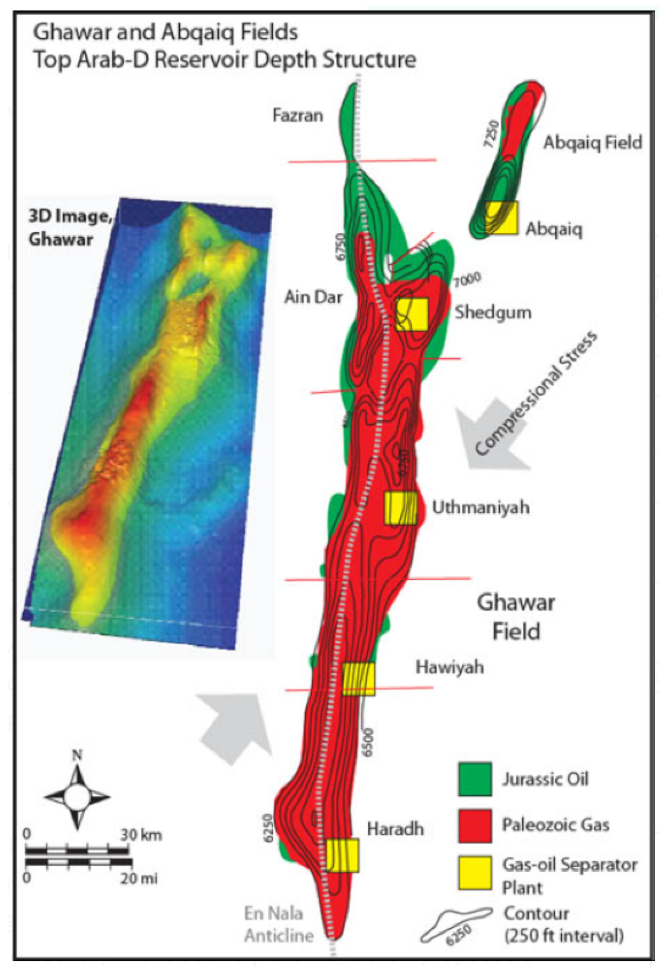
Figure 4.
A 3D illustration (with depths) of the Ghawar field showing the location of the gas and oil areas.
Figure 4.
A 3D illustration (with depths) of the Ghawar field showing the location of the gas and oil areas.

Figure 5.
Dolomite content in the Arab-D section of the Ghawar oilfield (reprinted/adapted with permission from [19]).
Figure 5.
Dolomite content in the Arab-D section of the Ghawar oilfield (reprinted/adapted with permission from [19]).

Figure 6.
Ghawar numerical model implemented in COMSOL with the studied well pattern.

Figure 7.
Equivalence between the real saturation profile (top) and the effective normalized saturation profile (bottom).
Figure 7.
Equivalence between the real saturation profile (top) and the effective normalized saturation profile (bottom).

Figure 8.
Schematic diagram of a shear-thinning/-thickening polymer solution, showing the viscoelastic behavior exhibited by these in porous media (reprinted/adapted with permission from [5]).
Figure 8.
Schematic diagram of a shear-thinning/-thickening polymer solution, showing the viscoelastic behavior exhibited by these in porous media (reprinted/adapted with permission from [5]).

Figure 9.
Porosity field of the Ghawar field used during the simulations.

Figure 10.
Absolute permeability field of the Ghawar field used during the simulations.

Figure 11.
Normalized saturation in the north of the Ghawar field for different mesh sizes.

Figure 12.
Overview and close-up of the elements distribution over the domain for the finer mesh.

Figure 13.
Normalized water saturation in the Ghawar field at four different time steps of the simulation.
Figure 13.
Normalized water saturation in the Ghawar field at four different time steps of the simulation.

Figure 14.
Normalized water saturation for different oil viscosities at the same timestep.

Figure 15.
Normalized polymer solution saturation at four different time steps of the simulation.

Figure 16.
Water-cut for the different producer wells as a function of time. Well #1 corresponds to the northernmost well, and well #4 to the southernmost one.
Figure 16.
Water-cut for the different producer wells as a function of time. Well #1 corresponds to the northernmost well, and well #4 to the southernmost one.

Figure 17.
Polymer solution viscosity in Ghawar field at four different time steps of the simulation.
Figure 17.
Polymer solution viscosity in Ghawar field at four different time steps of the simulation.

Figure 18.
Polymer solution rheological behavior as a function of the shear rate (a), and viscosity as a function of the polymer concentration (b).
Figure 18.
Polymer solution rheological behavior as a function of the shear rate (a), and viscosity as a function of the polymer concentration (b).

Figure 19.
Viscosity of the Ghawar field for polymer flooding without degradation (a,b) and with degradation (c,d).
Figure 19.
Viscosity of the Ghawar field for polymer flooding without degradation (a,b) and with degradation (c,d).

Figure 20.
Residence time distribution of particles in the field injected at the beginning of the simulation.
Figure 20.
Residence time distribution of particles in the field injected at the beginning of the simulation.

Figure 21.
Polymer concentration (a) and number of particles (b) at the producer wells as a function of time.
Figure 21.
Polymer concentration (a) and number of particles (b) at the producer wells as a function of time.

Figure 22.
Variation of the oil relative permeability as a function of the polymer flooding concentration (reprinted/adapted with permission from [50]).
Figure 22.
Variation of the oil relative permeability as a function of the polymer flooding concentration (reprinted/adapted with permission from [50]).

Figure 23.
Original and modified oil relative permeabilities, with a polymer concentration of 10 mol/m.
Figure 23.
Original and modified oil relative permeabilities, with a polymer concentration of 10 mol/m.

Figure 24.
Saturation (a) and corresponding recovery factor (b) for waterflooding, polymer flooding and modified polymer flooding for two different polymer concentrations.
Figure 24.
Saturation (a) and corresponding recovery factor (b) for waterflooding, polymer flooding and modified polymer flooding for two different polymer concentrations.


Table 1.
Porosity and permeability in the Ghawar oilfield [19].
Table 1.
Porosity and permeability in the Ghawar oilfield [19].
| Region | Porosity (%) | Permeability (mD) |
|---|---|---|
| Ain Dar | 19 | 617 |
| Shedgum | 19 | 639 |
| Uthmaniyah | 18 | 220 |
| Hawiyah | 17 | 68 |
| Haradh | 14 | 52 |
Table 2.
Element characteristics of different mesh sizes.
| Mesh Size | Number of Elements | Aver. Element Quality | Max. Element Size (km) | Min. Element Size (km) | Relative Error |
|---|---|---|---|---|---|
| Extremely coarse | 12,241 | 0.6348 | 11.5 | 0.365 | 0.70 |
| Extra coarse | 19,095 | 0.6554 | 6.78 | 0.261 | 0.20 |
| Coarser | 24,272 | 0.6784 | 4.53 | 0.208 | 0.32 |
| Coarse | 34,821 | 0.6985 | 3.49 | 0.156 | 0.42 |
| Normal | 54,834 | 0.7286 | 2.35 | 0.15 | 0.38 |
| Fine | 76,479 | 0.7457 | 1.82 | 0.0521 | 0.32 |
| Finer | 111,388 | 0.7684 | 1.46 | 0.0208 | 0.01 |
| Extra fine | 146,955 | 0.7905 | 0.678 | 0.00782 | 0.05 |
| Extremely fine | 298,688 | 0.8263 | 0.349 | 0.00104 | - |
Table 3.
Evaluation of shear-rate formulae.
| Eq. # | Formula | Shear Rate Value (1/s) |
|---|---|---|
| 1 | 35.307 | |
| 2 | 30.182 | |
| 3 | 42.684 |
Publisher’s Note: MDPI stays neutral with regard to jurisdictional claims in published maps and institutional affiliations. |
© 2022 by the authors. Licensee MDPI, Basel, Switzerland. This article is an open access article distributed under the terms and conditions of the Creative Commons Attribution (CC BY) license (https://creativecommons.org/licenses/by/4.0/).
Share and Cite
MDPI and ACS Style
Berger, M.; Picchioni, F.; Druetta, P. Simulation of Polymer Chemical Enhanced Oil Recovery in Ghawar Field. Energies 2022, 15, 7232. https://doi.org/10.3390/en15197232
AMA Style
Berger M, Picchioni F, Druetta P. Simulation of Polymer Chemical Enhanced Oil Recovery in Ghawar Field. Energies. 2022; 15(19):7232. https://doi.org/10.3390/en15197232
Chicago/Turabian StyleBerger, Maaike, Francesco Picchioni, and Pablo Druetta. 2022. "Simulation of Polymer Chemical Enhanced Oil Recovery in Ghawar Field" Energies 15, no. 19: 7232. https://doi.org/10.3390/en15197232
Note that from the first issue of 2016, this journal uses article numbers instead of page numbers. See further details here.