Robust Differentiator-Based NeuroFuzzy Sliding Mode Control Strategies for PMSG-WECS

Abstract

A robust control algorithm is always needed to harvest maximum power from a Wind Energy Conversion System (WECS) by operating it consistently at a Maximum Power Point (MPP) in the presence of wind speed variations. In this work, a Maximum Power Point Tracking (MPPT) control algorithm is designed via Conventional Sliding Mode Control (CSMC), the Super Twisting Algorithm (STA), and the Real Twisting Algorithm (RTA) and is applied to a Permanent Magnet Synchronous Generator (PMSG)-based WECS. CSMC is model-based whereas the STA and RTA are model-free controllers. In practice, the unavailability of nonlinear terms and aerodynamic forces deteriorates the performance of these controllers. Thus, an offline NeuroFuzzy algorithm is incorporated to estimate the nonlinear drift and control input channel to improve the robustness of these algorithms. In addition, the generator shaft speed and its missing derivative is recovered via a Uniform Robust Exact Differentiator (URED). In order to carry out a comprehensive comparative study among the three competitors, the overall system is simulated in a closed loop under the action of these controllers at three different operating conditions, i.e., nominal, varying load and inertia, and varying wind speed, using MATLAB/Simulink. The acquired results confirm the superiority of the RTA over the STA and CSMC in terms of robustness and chatter reduction.

1. Introduction

Over the past few decades, the wind turbine has become the most reliable and developed renewable energy source among its other counterparts. Based on wind speed, wind turbines are classified into fixed and variable speeds. However, the maximum power can be captured by employing a Variable-Speed Wind Turbine (VSWT). A VSWT, in contrast to a Fixed-Speed Wind Turbine (FSWT), which requires a power electronic converter for power flow control and a Maximum Power Point Tracking (MPPT) algorithm, and must be capable of delivering a high-quality electric power [1].

The most preferable options for VSWTs are the direct-drive Permanent Magnet Synchronous Generator (PMSG) and Doubly Fed Induction Generator (DFIG). The main advantages of the PMSG include a wide speed range (0–100 of the rated speed), high conversion efficiency, and high power density, due to its rare earth metal-based permanent magnets. This leads to a compact design, direct-drive, small-scale wind turbine with the ability to operate at very low speeds [2]. Currently, nine out of the top ten world manufacturers produce wind turbines with PMSGs [3].

Due to the rapid penetration of wind power in the electricity grid, it is essential to extract the maximum available power from the wind [4]. For this purpose, the Wind Energy Conversion System (WECS) needs to be operated consistently at the Maximum Power Point (MPP). This is accomplished through an MPPT control algorithm [5]. In this regard, several MPPT techniques have been proposed in the literature that can be categorized into three major types: Indirect Power Controller (IPC)-based algorithms, Direct Power Controller (DPC)-based algorithms, and other MPPT algorithms including fuzzy-based algorithms, Neural Network (NN)-based algorithms, adaptive algorithms, Multi-Variable Perturb and Observe (MVPO) algorithms, and SMC-based algorithms [4].

The IPC algorithm only boosts the mechanical wind power ($P_m$) and not the output electric power ($P_e$). IPC-based algorithms are subdivided into the Tip Speed Ratio (TSR) algorithm, Optimal Torque (OT) algorithm, and Power Signal Feedback (PSF) algorithm. In the TSR algorithm, the TSR is maintained at an optimum value at which the captured wind power is maximized by regulating the mechanical speed of the generator [6]. Although this algorithm is highly efficient, the need for an anemometer makes the system costlier. In the OT algorithm, the electromagnetic torque of the generator is controlled to obtain an optimum torque at a specified wind speed. Although this algorithm does not require the anemometer, it requires information on the turbine’s mechanical parameters as well as air density, which vary in different systems [7]. The PSF algorithm entails the knowledge of the wind turbine’s maximum power curve that is tracked by the control mechanism. Although this algorithm does not require the anemometer, it needs the parameters of the wind turbine [8].

The DPC-based algorithms, which directly maximize $P_m$, are further subdivided into the Hill Climbing Search (HCS) algorithm, Incremental Conductance (INC) algorithm, Optimal-Relation-Based (ORB) algorithm and hybrid algorithm [4]. HCS algorithms are sometimes, also termed Perturb and Observe ($P\&O$) algorithms. In this technique, if the operating point lies on the left side of the maximum point, the controller must shift it to the right to be closer to the maximum point, and vice versa. However, HCS needs to make an adjustment between the perturbation direction and tracking ability as well as between the step size and tracking speed [9]. The INC algorithm can perform better than the HCS algorithm in terms of providing maximum power extraction and efficiency. This algorithm does not require sensors and parameters of wind turbine and generator. This improves the system reliability and reduces the system cost [10]. The ORB algorithm requires knowledge of the system parameters as well as the optimum curve. These quantities are difficult to compute and may vary in practical applications [7]. A hybrid algorithm combines the advantages of two algorithms such as the ORB combined with $P\&O$ to provide a self-tuning capability [7].

Other MPPT algorithms include fuzzy-based algorithms, NN-based algorithms, adaptive algorithms, the MVPO algorithm, and SMC. The fuzzy and NN-based algorithms are also termed soft computing techniques. These are model-free algorithms and are independent of system parametric variations. However, the very large memory size requirement poses limitations in its implementation [11]. The adaptive algorithm renders an accurate optimal response. Furthermore, it can measure the uncertain system parameters [4]. The feedback linearization control based Particle Swarm Optimization (PSO) is suitable for WECS but is sensitive to varying parameters of the system and needs specific modeling of system [12]. Various nonlinear control schemes have been introduced to mitigate this issue. The smart control schemes such as neural network control [13,14], Takagi–Sugeno–Kang fuzzy control [11], and neural network [15] have been used to design an efficient controller for the WECS. However, these control approaches suffer from long offline training periods and time-consuming computations. Consequently, the SMC can be taken as an alternate option for the WECS owing to its simple design, insensitivity to parameter variations, order reduction, good robustness, disturbance rejection, and finite-time convergence [16,17,18]. However, the chattering problem is still a concerning issue that needs to be handled [19]. The Higher-Order Sliding Mode Control (HOSMC) technique needs the extra information regarding high order derivatives of sliding manifold and actuator may get damaged due to high gains [20].

In nutshell, the algorithms utilized for performance enhancement of the WECS either have compromised robustness mainly due to the unavailability of the nonlinear dynamics or compromised performance mainly due to the computationally intensive algorithms.

To tackle the aforementioned problems, an observer-based Conventional Sliding Mode Control (CSMC), the Super Twisting Algorithm (STA), and the Real Twisting Algorithm (RTA) have been proposed, giving fast and accurate MPPT for a WECS. The basic analogy of these three is the same as they tend to bring the system trajectories to a pre-defined sliding manifold, under the action of the discontinuous control law. On the sliding manifold, a system’s dynamics offer exciting advantages such as remarkable robustness against disturbances and parametric variations, and order reduction. To achieve these merits, the three algorithms have their own structures. The RTA has a simpler structure among the twisting algorithms and does not require a time derivative of a sliding function [21]. Moreover, the system trajectory can be asymptotically driven to the desired equilibrium point, while counteracting the disturbances. However, these algorithms are very sensitive to un-modeled fast dynamics, and chattering may appear sooner or later.

The novelty of the proposed control schemes is that the CSMC, STA, and RTA are modified to include an offline NeuroFuzzy estimator and a sliding modes-based Uniform Robust Exact Differentiator (URED). The NeuroFuzzy scheme gives estimates of the nonlinear drift and input channel while the URED provides a smoother estimate of the shaft speed and its missing derivatives. The merits added to the CSMC, STA and RTA include their excellent robust nature against parametric variations, external disturbances, and capability to substantially handle chattering in the case of the STA and RTA.

This paper is structured into the following sections. In Section 2, mathematical modeling of WECS is presented. Section 3 describes the normal form conversion of the system states. In Section 4, the generator shaft velocity and its missing derivative are recovered via a Uniform Robust Exact Differentiator (URED). The offline NeuroFuzzy algorithm is designed for the estimation of nonlinear terms in Section 5. The proposed control schemes are covered in detail in Section 6, while simulation results are discussed in Section 7. Finally, Section 8 comments on the conclusion and presents potential applications where the results of this research can be used.

2. Wind Energy Conversion System

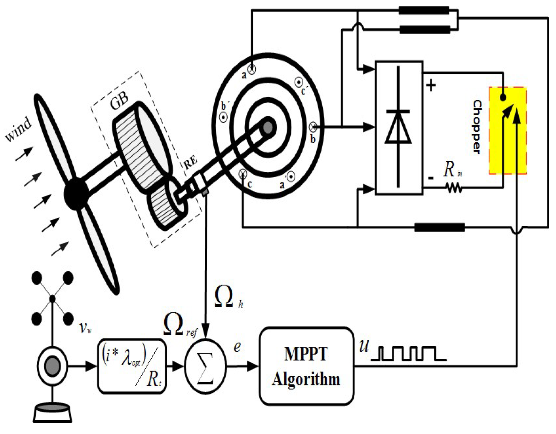
A Wind Energy Conversion System (WECS) includes the aerodynamic model of the wind turbine and a model of the PMSG connected to the load. The schematic of the designed PMSG-based WECS along with the controller part is depicted in Figure 1.

2.1. Wind Turbine Model

The details regarding the mathematical modeling are adopted from [12]. The mechanical power available at the turbine shaft is expressed in (1),

$$\begin{array}{c}\hfill p_m=\frac{1}{2}\rho \pi R_t^2{v_w}^3{C}_p\left(\lambda \right)\end{array}$$

(1)

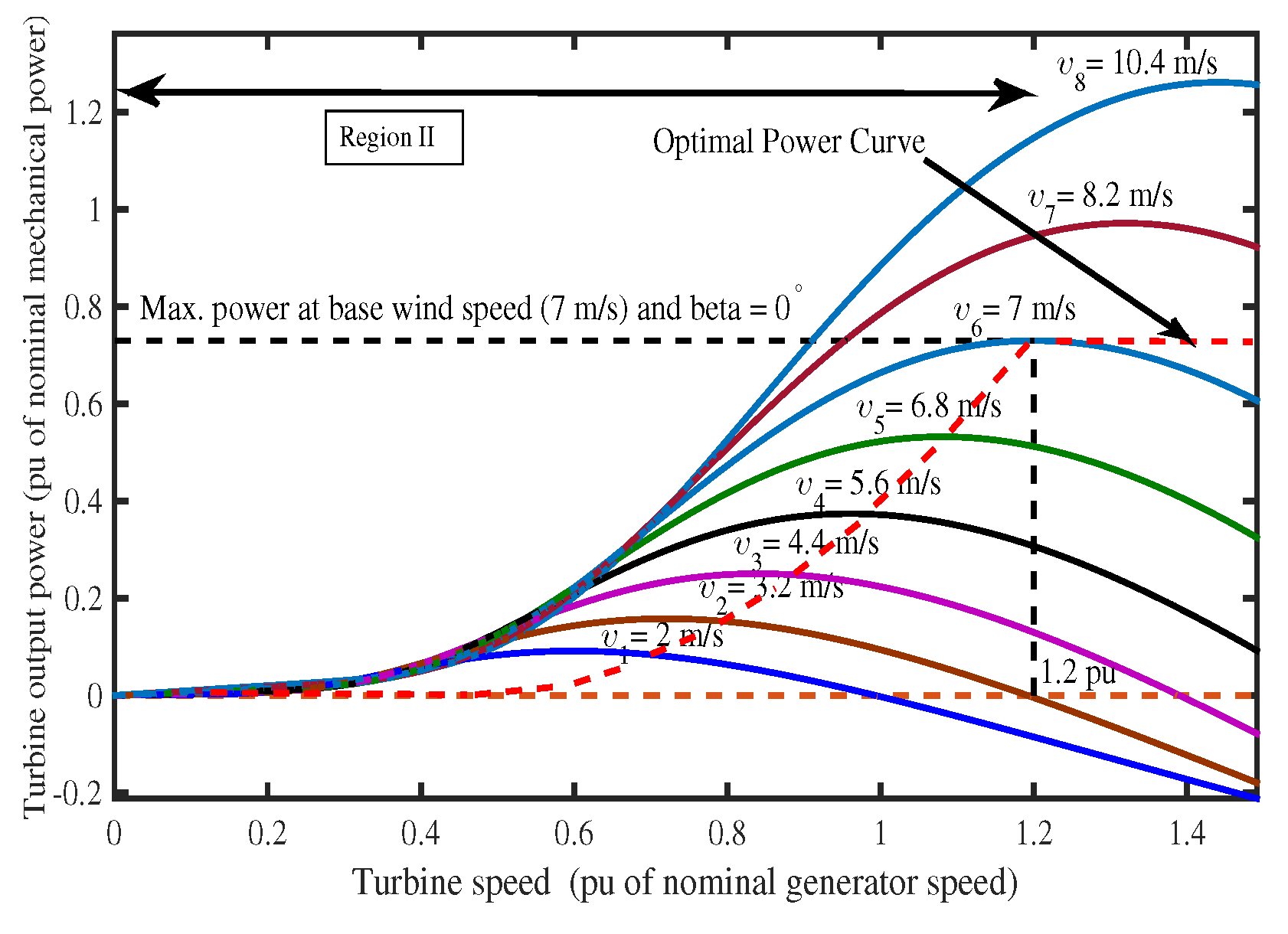
where $\rho$ is the air mass-density, $R_t$ is the radius of the turbine blade, $R_t^2$ is the swept area of the turbine, $v_w$ is the wind speed, with an average value of $7m/s$ as depicted in Figure 2, $C_p$ is the power coefficient, indicating the efficiency of the wind turbine, and $\lambda$ is the TSR, which is given by the subsequent expression (2):

$$\begin{array}{c}\hfill \lambda =\frac{{\mathsf{\Omega }}_h{R}_t}{v_{w}i}\end{array}$$

(2)

where ${\mathsf{\Omega }}_h$$(rad/s)$ is the High-Speed Shaft (HSS) angular speed of the turbine and i is the transmission ratio. The typical parameters are given in

Table 1. Parameters of the system [12] and controller.

Type	Name of Parameter	Magnitude
Turbine	Air mass density, $\rho$	1.25 kg/m${}^3$
	Turbine blade radius, $R_t$	2.5 m
	Optimum tip speed ratio, ${\lambda }_{opt}$	7
	Transmission ratio, i	7
	Maximum power coefficient, $C_{p_{max}}$	0.476
PMSG	Stator resistance, $R_s$	3.3 $\mathsf{\Omega }$
	Stator d axis inductance, $L_d$	0.0416 H
	Stator q axis inductance, $L_q$	0.0416 H
	Flux, $\varphi$	0.04382 Wb
	Pole pair, p	3
	High-speed shaft inertia, $J_{HSS}$	0.0552 kg/m${}^2$
	Load inductance, $L_{ch}$	0.08 H
Controller	Constant, ${\mathsf{{\rm Y}}}_1$	1000
	Constant, ${\mathsf{{\rm Y}}}_2$	0.01
	Constant, $k_1$	60
	Constant, $k_2$	1000
	Constant, ${\beta }_1$	80
	Constant, ${\beta }_2$	15
URED	Constant, ${\alpha }_1$	36
	Constant, ${\alpha }_2$	1000
	Constant, ${\alpha }_3$	1
	Constant, ${\alpha }_4$	1800

.

The wind-power coefficient $C_p\left(\lambda \right)$ is a nonlinear function of TSR and pitch angle. It reaches the maximum when the TSR is at the optimum value, known as ${\lambda }_{opt}$. Therefore, a variable-speed wind turbine monitors the $C_{P_{max}}$ to extract the maximum power up to the nominal speed by changing the rotor-shaft speed to keep the system at ${\lambda }_{opt}$.

$$\begin{array}{c}\hfill C_p\left(\lambda \right)=(6.1\lambda -1.3{\lambda }^2+8.1{\lambda }^3-0.97477{\lambda }^4){10}^{-3}\end{array}$$

(3)

The wind turbine delivers a mechanical torque, to the rotor shaft, according to the following expression.

$$\begin{array}{c}\hfill {\mathsf{\Gamma }}_m=\frac{1}{2}\rho \pi R_t^3{v_w}^2{C}_T\left(\lambda \right)\end{array}$$

(4)

where $C_T\left(\lambda \right)$ is the torque-coefficient which is given by the following form.

$$\begin{array}{c}\hfill C_T\left(\lambda \right)=\frac{C_p\left(\lambda \right)}{\lambda }\end{array}$$

(5)

All the necessary details are now reported and it is convenient to present the mathematical modeling of the PMSG.

2.2. PMSG Modeling

The PMSG modeled in the $dq$-axes is given as follows [12].

$$\begin{array}{ccc}\hfill \frac{d{i}_d}{dt}& =& \hfill \frac{-R_s{i}_d+p(L_q-L_{ch}){\mathsf{\Omega }}_h{i}_q-R_{ch}{i}_d}{(L_d+L_{ch})}\hfill \\ \hfill \frac{d{i}_q}{dt}& =& \hfill \frac{-R_s{i}_q-p(L_q+L_{ch}){\mathsf{\Omega }}_h{i}_d-R_{ch}{i}_q}{(L_q+L_{ch})}+p{\mathsf{\Omega }}_h\mathsf{\Phi }\hfill \\ \hfill \frac{d{\mathsf{\Omega }}_h}{dt}& =& \hfill \frac{1}{\left(J_{HSS}\right)}\left[-p\mathsf{\Phi }{i}_q+\frac{d_1{v}_w^2}{i}+\frac{d_2{v}_w{\mathsf{\Omega }}_h}{i^2}+\frac{d_3{\mathsf{\Omega }}_h^2}{i^3}\right]\hfill \end{array}$$

(6)

where $R_s$ is the stator resistance, $L_d$ and $L_q$ are the stator inductances for a non-salient pole PMSG (i.e., $L_d$=$L_q$) along d and q axis, respectively, p is the pole pair, ${\mathsf{\Omega }}_h$ is the high speed shaft angular speed of the rotor shaft, $\mathsf{\Phi }$ is the constant flux, i is the transmission ratio, $J_{HSS}$ is the high speed shaft inertia, and $i_d$ and $i_q$ are the stator currents along d and q axis, respectively. Using the conventional terms for some of these quantities, i.e.,

$$\begin{array}{ccc}\hfill i_d& =& \hfill x_1\hfill \\ \hfill i_q& =& \hfill x_2\hfill \\ \hfill {\mathsf{\Omega }}_h& =& \hfill x_3\hfill \end{array}$$

Thus, a simplified state space equation of the system, in terms of the above parameters, can be written as,

$$\begin{array}{c}\hfill \left[\begin{array}{c}{\dot{x}}_1\\ {\dot{x}}_2\\ {\dot{x}}_3\end{array}\right]=\left[\begin{array}{c}-(a_1+a_3{R}_{ch})-\left(a_2{x}_3\right)+0\\ -\left(c_2{x}_3\right)-(c_1+c_4{R}_{ch})+c_3\\ \frac{k_1{v}^2}{x_1}-k_4-(k_{2}v+k_3{x}_3)\end{array}\right]\left[\begin{array}{c}{x}_1\\ x_2\\ x_3\end{array}\right]\end{array}$$

(7)

The values of the constants $a_1=c_1=R_s/(L_d+L_{ch})$, $a_2=p(L_q-L_{ch}/(L_d+L_{ch})$, $a_3=c_4=1/(L_d+L_{ch})$, $c_2=p$, $c_3=k_4=p\varphi$, $k_1=d_1/\left(i{J}_{HSS}\right)$, $k_2=d_2/\left(i^2{J}_{HSS}\right)$, and $k_3=d_3/\left(i^3{J}_{HSS}\right)$ are listed in

Table 2. Parameters specifications.

Parameter	Value	Parameter	Value	Parameter	Value
$a_1$	$27.147$	$c_1$	$27.147$	$k_1$	$9.945$
$a_2$	$0.94866$	$c_2$	3	$k_2$	$0.1332$
$a_3$	$8.2264$	$c_3$	$1.3146$	$k_3$	$0.00506$
$a_4$	0	$c_4$	$8.2264$	$k_4$	$23.806$

.

3. Normal Form Conversion

The nonlinear PMSG-WECS model in (7) can be expressed as [12],

$$\begin{array}{ccc}\hfill \dot{x}& =& \hfill f\left(x\right)+g\left(x\right)u+\mathsf{\Delta }(x,t)\hfill \\ \hfill y& =& \hfill h\left(x\right)\hfill \end{array}$$

(8)

where x∈$R^n$ represents the state vector, u is the control input, $\mathsf{\Delta }(x,t)$ is matched uncertainty, while $f\left(x\right)$ and $g\left(x\right)$ are nonlinear smooth vector fields which have the following expressions

$$\begin{array}{ccc}\hfill f\left(x\right)& =& \hfill \left[\begin{array}{c}\hfill f_1\hfill \\ \hfill f_2\hfill \\ \hfill f_3\hfill \end{array}\right]=\left[\begin{array}{c}-a_1{x}_1-a_2{x}_2{x}_3\\ -c_1{x}_2-c_2{x}_1{x}_3+c_3{x}_3\\ -k_1{v}^2-k_{2}v{x}_3-k_3{x}_3^2-k_4{x}_2\end{array}\right]\hfill \\ \hfill g\left(x\right)& =& \hfill \left[\begin{array}{c}\hfill -a_3{x}_1\hfill \\ \hfill -c_4{x}_2\hfill \\ \hfill 0\hfill \end{array}\right]\hfill \end{array}$$

and

$$\begin{array}{c}\hfill u=R_{ch}\end{array}$$

The output, y=$h\left(x\right)$=$x_3$=${\mathsf{\Omega }}_h$ is the angular speed of the rotor shaft. Since the objective is to control ${\mathsf{\Omega }}_h$, therefore, (7) can be transformed into input–output form by defining the following transformation.

$$\begin{array}{ccc}\hfill z_1& =& \hfill y=h\left(x\right)=x_3={\mathsf{\Omega }}_h\hfill \\ \hfill z_2& =& \hfill L_{f}h\left(x\right)=\frac{\partial h\left(x\right)}{\partial x}f\left(x\right)=-{\phi }_1-{\phi }_2{x}_3-{\phi }_3{x}_3^2-{\phi }_4{x}_2\hfill \\ \hfill z_3& =& \hfill L_f^{2}h\left(x\right)=\frac{x_1}{x_2}\hfill \end{array}$$

(9)

where

$\hspace{1em}\hspace{1em}\hspace{1em}\hspace{1em}\hspace{1em}{\phi }_1$ = $k_1{v}_w^2$, ${\phi }_2$=$k_2{v}_w$, ${\phi }_3$=$k_3$ and ${\phi }_4$=$k_4$

The relative degree (r) of the system is one less than the system order ($n=3$), i.e., ($r<n$), so the input–output form appears as follows.

$$\begin{array}{c}\hfill \left.\begin{array}{cc}\hfill {\dot{z}}_1& \hfill =z_2\hfill \\ \hfill {\dot{z}}_2& \hfill =L_f^{2}h\left(x\right)+L_g{L}_{f}h\left(x\right)u\hfill \end{array}\right\}\end{array}$$

(10)

$$\begin{array}{c}\hfill {\dot{z}}_3=\frac{{\phi }_4}{{\phi }_1}(-\frac{a_1{z}_3{\phi }_1}{{\phi }_4}-\frac{a_2{z}_1{\phi }_1}{{\phi }_4}-\frac{a_3{x}_1{z}_3{\phi }_{1}u}{{\phi }_4})\hfill \\ \hfill \hspace{1em}\hspace{1em}\hspace{1em}\hspace{1em}\hspace{1em}\hspace{1em}\hspace{1em}\hspace{1em}-\left(\frac{z_3{\phi }_1}{{\phi }_4}\right)\left(\frac{{\phi }_4^2}{{\phi }_1^2}\right)(-\frac{a_1{\phi }_1}{{\phi }_4}-\frac{c_2{\phi }_1{z}_3{z}_1}{{\phi }_4}+k_4{z}_1-\frac{a_3{x}_1{\phi }_{1}u}{{\phi }_4})\end{array}$$

(11)

where

$$\begin{array}{c}\hfill \left.\begin{array}{c}\hfill L_f^{2}h\left(x\right)=-{\phi }_4{f}_2\left(x\right)-({\phi }_2+2{\phi }_3{x}_3)f_3\left(x\right)\\ \hfill L_g{L}_{f}h\left(x\right)=a_3{x}_1{\phi }_4{x}_2\end{array}\right\}\end{array}$$

(12)

The dynamics shown in (11) represent the internal dynamics that are indirectly affected by the control input. Now, it is required to prove the stability of the zero dynamics. The nonlinear system dynamics are divided into two parts, i.e., an internal part and an external (input-output) part when performing the input–output conversion. Since the external dynamic states i.e., $(z_1$, $z_2)$ are controllable states, i.e., they can be directly controlled by u while the stability of the internal dynamic state, i.e., $z_3$ is simply determined by the location of zeros [22]. To obtain the zero dynamics, set $z_1$ = $z_2$ = u = 0 in (11). Consequently, one gets

$$\begin{array}{c}\hfill {\dot{z}}_3=-z_3(k_1-a_1)\end{array}$$

(13)

This confirms that the zero dynamics are stable as long as $k_1>a_1$.

4. Uniform Robust Exact Differentiator

It is worthy to mention that in practical implementation, the forthcoming control technique will need the higher derivatives of the output (and the derivative of the sliding surface in the case of the real twisting controller). Therefore, these derivatives will be estimated in this work via the Uniform Robust Exact Differentiator (URED). Assume that the actual available output is $z_1$ while ${\widehat{z}}_1$ is its estimated value.

Suppose that the output $z_1$ is twice differentiable with a second derivative bounded by constant $L>0$. The mismatch between the actual and estimated output (in a noise-free case) is as follows,

$$\begin{array}{c}\hfill \xi ={\widehat{z}}_1-z_1\end{array}$$

(14)

Now, the estimated output ${\widehat{z}}_1$ and its estimated derivative ${\widehat{z}}_2$ can be computed via the solution of the following second-order system, the so-called uniform exact differentiator [23].

$$\begin{array}{c}\hfill \left.\begin{array}{cc}\hfill {\widehat{\dot{z}}}_1& \hfill =-{\alpha }_1{\psi }_1+{\widehat{z}}_2\hfill \\ \hfill {\widehat{\dot{z}}}_2& \hfill =-{\alpha }_2{\psi }_2\hfill \end{array}\right\}\end{array}$$

(15)

where ${\alpha }_1$ and ${\alpha }_2$ are positive input gains and ${\psi }_1$ and ${\psi }_2$ are the injecting terms which are expressed (in terms of $\xi$) as follows.

$$\begin{array}{c}\hfill {\psi }_1=-{\alpha }_3{\left|\xi \right|}^{0.5}sign\left(\xi \right)-{\alpha }_4{\left|\xi \right|}^{3/2}sign\left(\xi \right)\end{array}$$

(16)

and

$$\begin{array}{c}\hfill {\psi }_2=-0.5{\alpha }_3^{2}sign\left(\xi \right)-2{\alpha }_3{\alpha }_4\xi -3/2{\alpha }_4^2{\left|\xi \right|}^{2}sign\left(\xi \right)\end{array}$$

(17)

Note that ${\alpha }_3$ and ${\alpha }_4$ are positive constants and the high degree terms ${\left|\xi \right|}^{3/2}sign\left(\xi \right)$ and ${\left|\xi \right|}^{2}sign\left(\xi \right)$ provide uniform convergence independent of the initial conditions.

5. NeuroFuzzy Algorithm-Based Nonlinear Functions Estimation

In this section, a NeuroFuzzy algorithm based on the Takagi–Sugeno–Kang (TSK) fuzzy inference system (as shown in Figure 3) is used to generate/estimate the nonlinear functions $L_f^{2}h\left(x\right)$ and $L_g{L}_{f}h\left(x\right)$. The variables $z_1$, $z_2$, $z_3$, and the wind speed $v_w$ are the main inputs to the system, whereas the final outputs are the estimates of $L_f^{2}h\left(x\right)$ or $L_g{L}_{f}h\left(x\right)$, i.e., this is a Multi-Input Single-Output (MISO) structure. The overall NeuroFuzzy estimation network is comprised of multiple layers which will be discussed in the forthcoming paragraphs.

The first layer consists of all the inputs which are available during the estimation process. The second layer develops the membership functions which are based on the Gaussian function, i.e., the membership functions can be calculated as follows,

$$\begin{array}{c}\hfill {\mu }_{ij}=e^{\frac{{(x_j-c_{ij})}^2}{{\sigma }_i^2}}\end{array}$$

(18)

where j represents the number of inputs, i points to the number of fuzzy rules, and $c_{ij}$ and ${\sigma }_i^2$ refers to the center and width of the $i_{th}$ Gaussian function, respectively. Since the proposed adaptive NeuroFuzzy structure and architecture depend upon the $IF-THEN$ rules. For example, it works by the architecture,

$$\begin{array}{c}\hfill R_i:If{x}_{i1}is{\mu }_{i1}\mathrm{AND}{x}_{i2}is{\mu }_{i2}\mathrm{and}\cdots \\ \hfill \mathrm{and}{x}_{ij}is{\mu }_{ij}THEN{z}_i={\mathsf{\Psi }}_i{a}_{ij}\end{array}$$

In the third layer, each node represents the antecedent connective part of the extracted $IF-THEN$ fuzzy rule which can be expressed by the following mathematical expression.

$$\begin{array}{c}\hfill R_i=\prod _{j=1}^{n+m}{\mu }_{ij}=e^{{\sum }_{j=1}^{n+m}\frac{{(x_j-c_{ij})}^2}{{\sigma }_i^2}}\end{array}$$

(19)

The fourth layer is the normalization layer which provides the normalized value via the following expression.

$$\begin{array}{c}\hfill {\mathsf{\Psi }}_i=\frac{R_i}{{\sum }_i{R}_i}\end{array}$$

(20)

The fifth layer, based on the outputs of the fourth layer, is the summation layer which integrates all the normalized values of layer four and provides an estimated value via the following expression.

$$\begin{array}{c}\hfill L_f^{2}h\left(x\right)=\frac{{\sum }_i{\prod }_{i=1}^m{\mu }_{ij}{a}_i}{{\sum }_i{\prod }_{i=1}^m{\mu }_{ij}}=\frac{{\sum }_i{R}_i{a}_i}{{\sum }_i{R}_i}={\mathsf{\Psi }}_i{a}_i\end{array}$$

(21)

where $a_i$ is a constant parameter which shows the $i_{th}$ rule consequence. Now, the nonlinear terms are estimated and are ready to be utilized in the controller algorithm.

6. MPPT Control Design Strategies

In the previous sections, the control convenient form (i.e,. normal form) and nonlinear terms, i.e., $L_f^{2}h\left(x\right)$ and $L_g{L}_{f}h\left(x\right)$ were estimated. Now, the main objective is to extract the maximum power from the plant by designing a proper and well-suited MPPT control algorithm. This task is done here via the CSMC, the super twisting control law, and the real twisting control law with the configuration shown in Figure 4.

6.1. Conventional Sliding Mode Control Design

The design of the CSMC is pursued by first defining a switching surface in terms of errors (a mismatch between the actual and desired states) followed by defining a discontinuous control law that enforces sliding modes along the surface.

The attractiveness lies in the fact that once the system state variables influence the switching surface, the structure of the feedback loop is adaptively altered, and the system states slide along the switching manifold. A system in sliding mode progresses with $n-m$ number of states with n being the dimension of system states and m being the dimension of control inputs. This order reduction provides invariance to the plant parameter variations and the disturbances which is one of the main benefits of SMC. Now the control design, for the reference tracking, can be carried out by defining the tracking error, $e\left(t\right)$, as follows,

$$\begin{array}{c}\hfill e\left(t\right)=z_1-{\mathsf{\Omega }}_{ref}\left(t\right)\end{array}$$

(22)

For the sake of ease, ${\mathsf{\Omega }}_{ref}\left(t\right)$ will be represented by $z_{1ref}$ for the rest of the paper. Now, the time derivative of (22) becomes,

$$\begin{array}{c}\hfill \dot{e}\left(t\right)={\dot{z}}_1-{\dot{z}}_{1ref}\end{array}$$

(23)

In the actual implementation, only $z_1$ is available and its derivative is estimated via a Uniform Robust Exact Differentiator (URED). Therefore, ${\dot{z}}_1$ will be replaced by ${\widehat{z}}_2$ (i.e., estimated derivative of $z_1$). Thus,

$$\begin{array}{c}\hfill \dot{e}\left(t\right)={\widehat{z}}_2-{\dot{z}}_{1ref}\end{array}$$

(24)

Further differentiation of (24) along (10) and (11) becomes

$$\begin{array}{c}\hfill \ddot{e}\left(t\right)={{\widehat{L}}_f}^{2}h\left(x\right)+{\widehat{L}}_g{L}_{f}h\left(x\right)u\end{array}$$

(25)

The sliding manifold of a PI type is defined as follows:

$$\begin{array}{c}\hfill s=({\widehat{z}}_2-{\dot{z}}_{1ref})+{\alpha }_1(z_1-z_{1ref})\cdots \\ \hfill +{\alpha }_2{\int }_0^t(z_1-z_{1ref})d\tau \end{array}$$

(26)

where ${\alpha }_1$ and ${\alpha }_2$ are the positive gains. The time derivative of (26) along (10) and (11) becomes

$$\begin{array}{c}\hfill \dot{s}=({\dot{\widehat{z}}}_2-{\ddot{z}}_{1ref})+{\alpha }_1({\widehat{z}}_2-{\dot{z}}_{1ref})+{\alpha }_2(z_1-z_{1ref})\end{array}$$

(27)

The values of ${\dot{\widehat{z}}}_2$ are considered similar to the second equation of (10) in which $L_f^{2}h\left(x\right)$ and $L_g{L}_{f}h\left(x\right)$ are replaced with their estimated values performed in the previous section.

In this strategy, the strong reachability of the following form is considered.

$$\begin{array}{c}\hfill \dot{s}=-k_{1}s-k_{2}sign\left(s\right)\end{array}$$

(28)

Now comparing (27) and (28), one gets,

$$\begin{array}{c}\hfill u=\frac{1}{{\widehat{L}}_g{L}_{f}h\left(x\right)}[{\ddot{z}}_{1ref}-{\alpha }_1{\widehat{z}}_2-{\alpha }_2{z}_1+{\alpha }_1{\dot{z}}_{1ref}...\\ \hfill +{\alpha }_2{z}_{1ref}-{\widehat{L}}_f^{2}h\left(x\right)-k_{1}s-k_{2}sign\left(s\right)]\end{array}$$

(29)

where, $k_1$ and $k_2$ are the positive gains of the control input u.

To prove the closed loop stability, with the proposed PI sliding surface, the time derivative of a Lyapunov candidate function $v=\frac{1}{2}{s}^2$ along (27) and (29) becomes,

$$\begin{array}{ccc}\hfill \dot{v}& =& \hfill s\dot{s}\hfill \\ \hfill \dot{v}& =& \hfill -k_1{s}^2-k_{2}ssign\left(s\right)\hfill \\ \hfill \dot{v}& \le & \hfill -k_1{s}^2-k_2\left|s\right|\hfill \end{array}$$

(30)

The inequality in (30) indicates the finite time enforcement of sliding modes. Note that this is the conventional control law based on the PI surface, which maintains sliding mode from the very start (i.e., $t\ge 0$) (confirmed by (30)). It also confirms that the system evolves with full states in sliding mode. Now, to reduce the chattering across the sliding manifold, the HOSM control strategies (i.e., super twisting and real twisting) are designed.

6.2. Super Twisting Algorithm Design

The CSMC suffers from high-frequency oscillations across the switching manifold which can cause problems in any practical application. As a remedy to eradicate such oscillations, among many techniques, the higher-order sliding modes based on smooth switching law, known as the Super Twisting Algorithm (STA), is utilized.

$$\begin{array}{c}\hfill \dot{s}=u_t=-{\beta }_1{\left|s\right|}^{0.5}sign\left(s\right)-{\beta }_2\int sign\left(s\right)dt\end{array}$$

(31)

where ${\beta }_1$ and ${\beta }_2$ are positive scalars. By comparing (27) and (31), one may get the following sliding mode enforcement law.

$$\begin{array}{c}\hfill u_{st}=u_{eqv}+u_t\end{array}$$

(32)

where $u_{eqv}$ is the equivalent controller defined in (29). It is worth noting that due to the variable gain of the first term in $u_t$, the gain decreases as the trajectories strike towards the manifold while in the second term, the integral provides a low pass filtering effect. This causes a considerable reduction in chattering.

Now, in the next subsection, we use real twisting law to suppress the chattering. The closed-loop stability remains almost similar to the one outlined in the CSMC presentation.

6.3. Real Twisting Control Algorithm Design

As mentioned earlier, the chattering is undesirable in electro-mechanical systems because it actuates high-frequency dynamics which can cause instability, and wear/tear of the system [24]. This is considerably alleviated via the use of STA. However, the STA is still sensitive to un-modeled fast dynamics due to which chattering may appear sooner or later in the system [19]. To deal with this, a model-free second-order sliding mode control law named the Real Twisting Algorithm (RTA) is used. The overall discontinuous control law, $u_r$, is given as,

$$\begin{array}{c}\hfill u_r=-{\mathsf{{\rm Y}}}_{1}sign\left(s\right)-{\mathsf{{\rm Y}}}_{2}sign\left(\dot{s}\right)\end{array}$$

(33)

where s is defined in (26) while the gains ${\mathsf{{\rm Y}}}_1$ and ${\mathsf{{\rm Y}}}_2$ are positive constants. These gains are often chosen by trial and error. For more details, the readers may see [25].

7. Results and Discussion

The PMSG-based WECS (depicted in Figure 1), along with the proposed control scheme, is depicted in Figure 4. The PMSG-based WECS, under consideration, has a maximum power coefficient $C_{p_{max}}=0.476$, that corresponds to an optimal TSR ${\lambda }_{opt}=7$. The remaining relevant parameters are listed in Table 1. Moreover, an optimal wind speed (7 m/s, see Figure 2) is considered for simulations. The efficacy of the proposed algorithm is evaluated, via comparison with CSMC and STA, in three distinct cases: nominal, varying load and varying inertia, and deterministic.

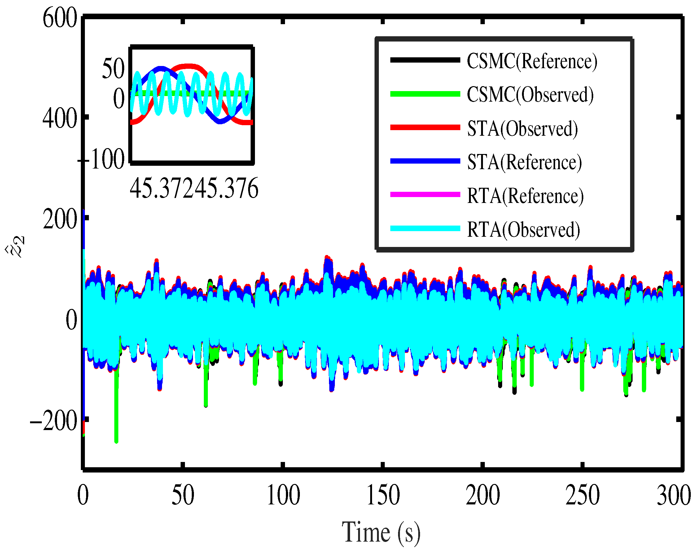
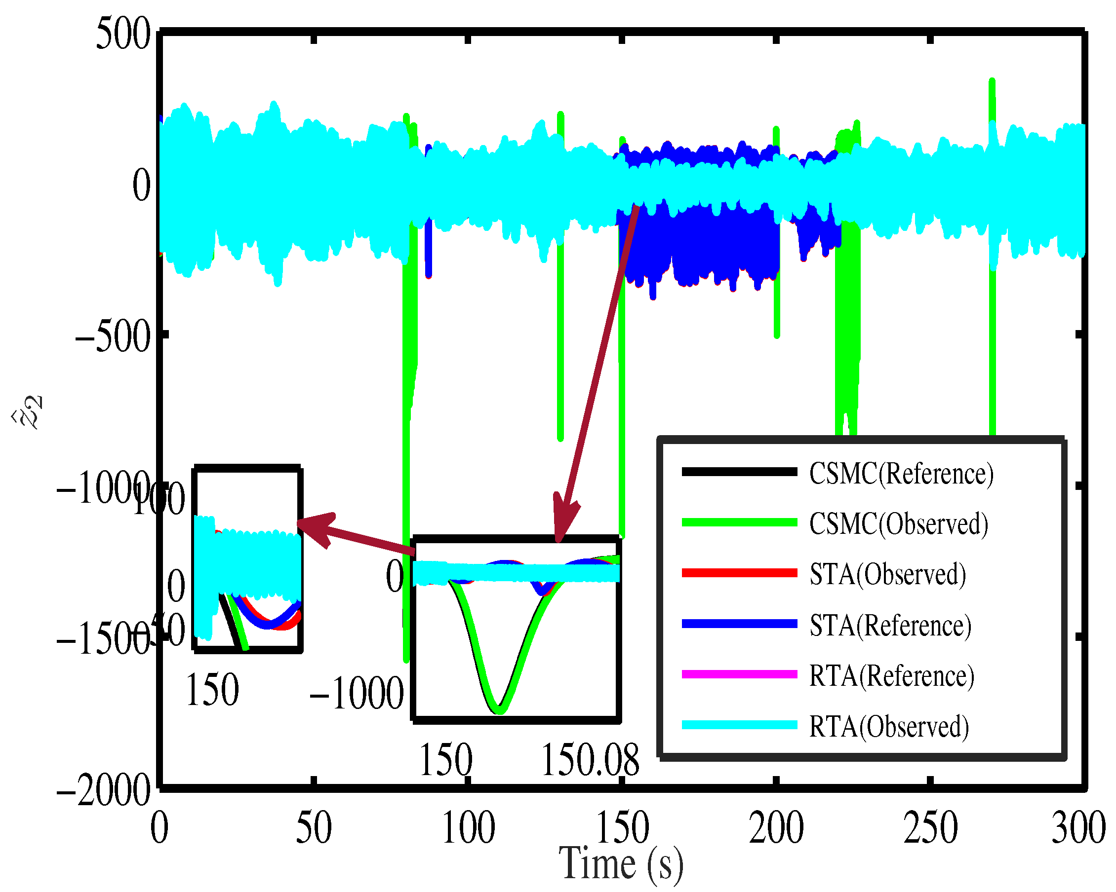
In the nominal case, the MPPT is subjected to a stochastic wind speed profile. In the load-varying inertia case, the robustness of the proposed control scheme is analyzed under a stochastic wind speed profile with varying load and inertia. Finally, the robust performance, in the presence of abrupt variations in wind speed profile, is evaluated. Moreover, the URED observed states in the nominal and in varying load varying inertia case are shown in Figure 5 and Figure 6, respectively. It must be observed that due to the continuous nature of STA and RTA, the performance of URED is better than that of CSMC. In the case of CSMC, the undershoots are caused by the presence of chattering in the reference signal. Moreover, since the overall performance depends upon these estimates thus, better performance is expected in the case of STA and RTA. In addition, the estimated data comply with the standards of a physical system and thus stand validated with the knowledge of a real/practical system.

7.1. Nominal Case

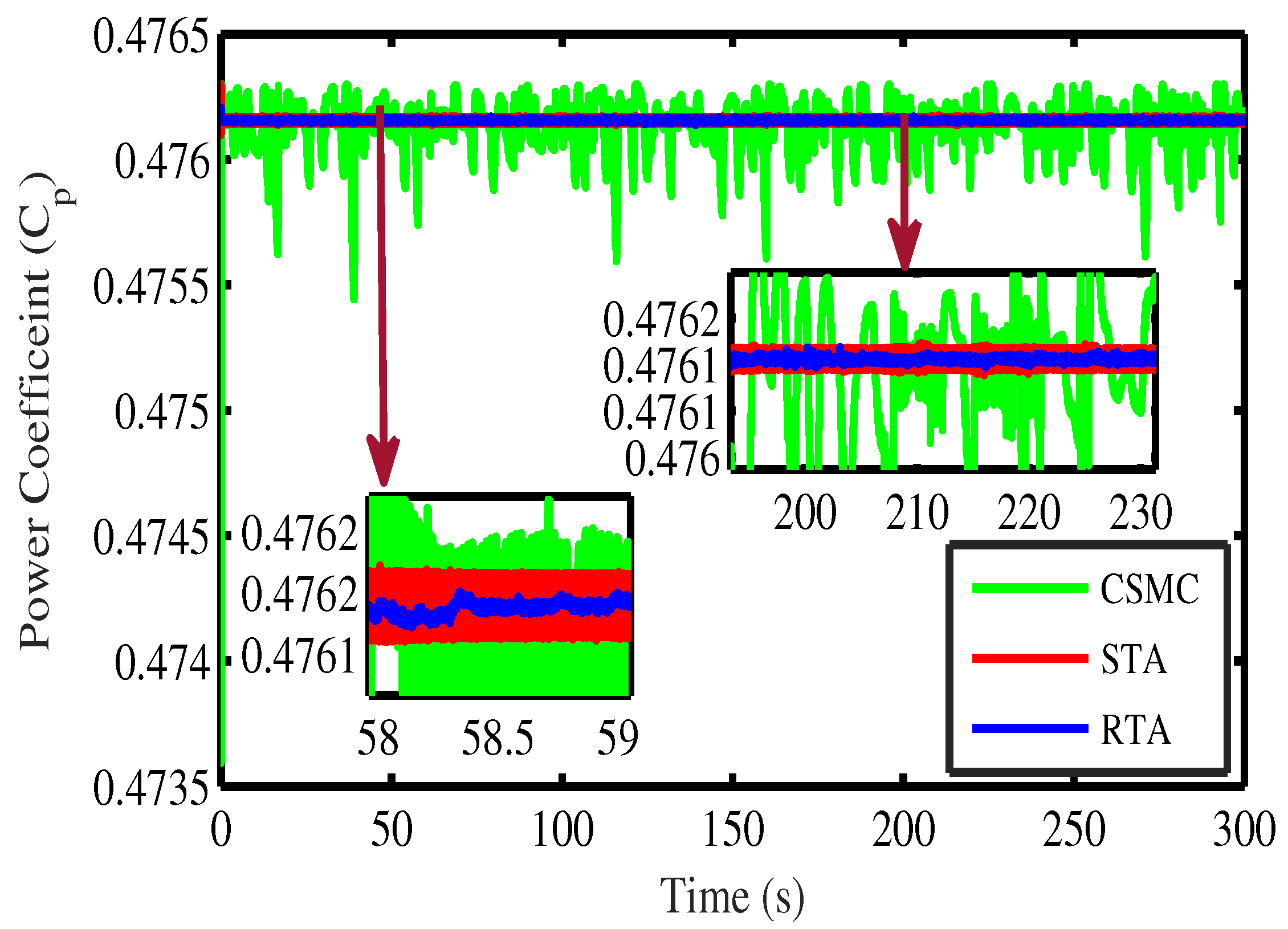
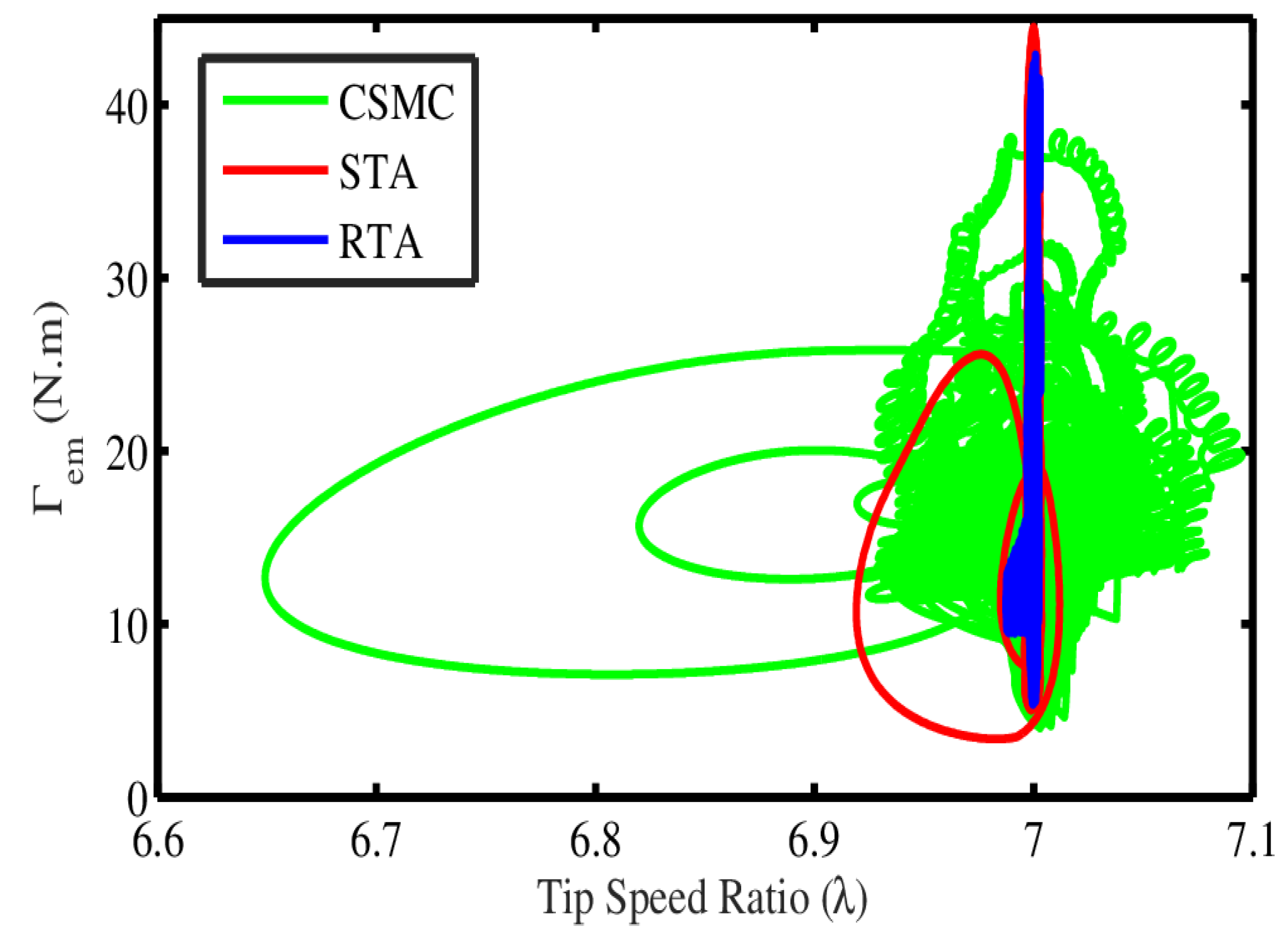
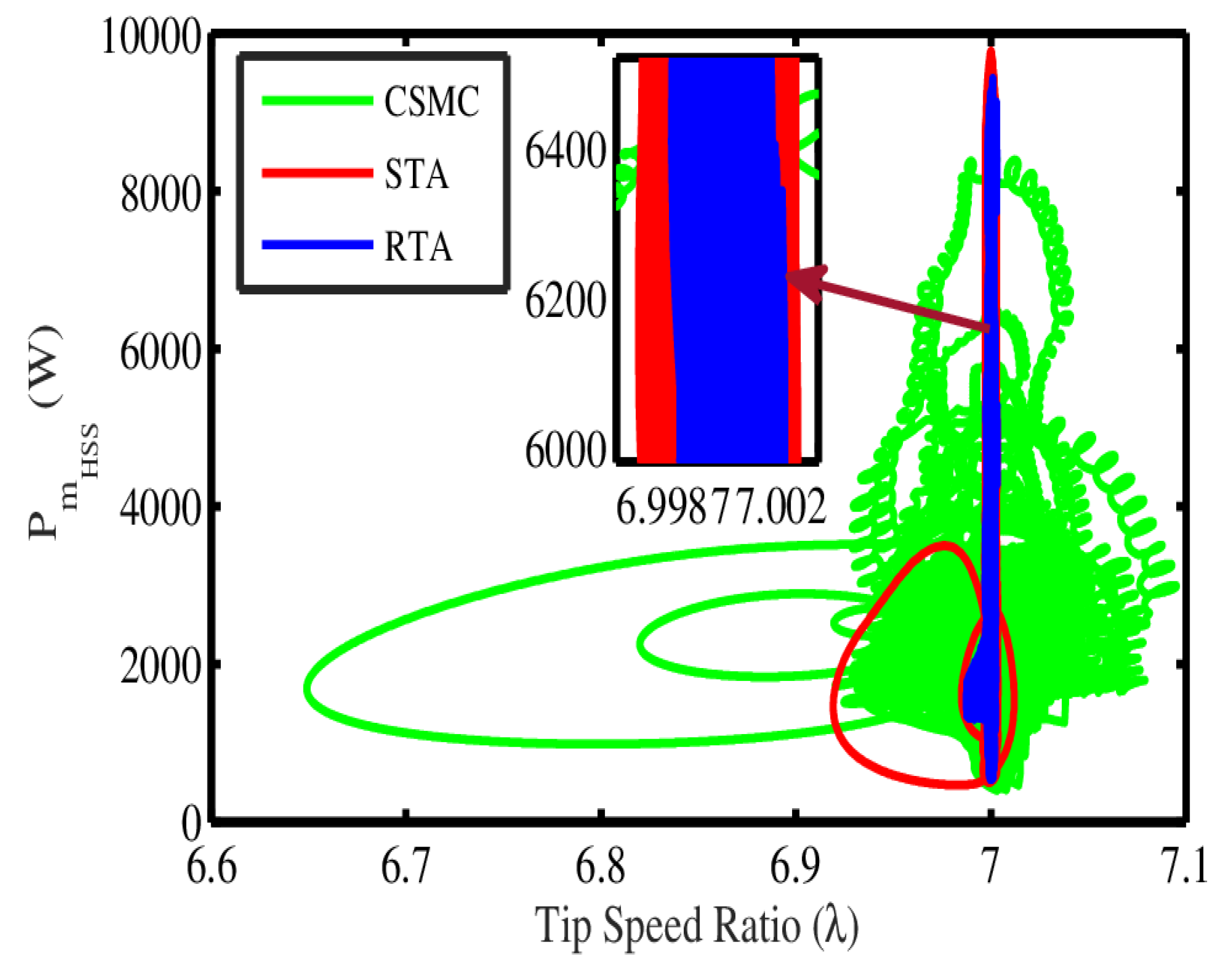
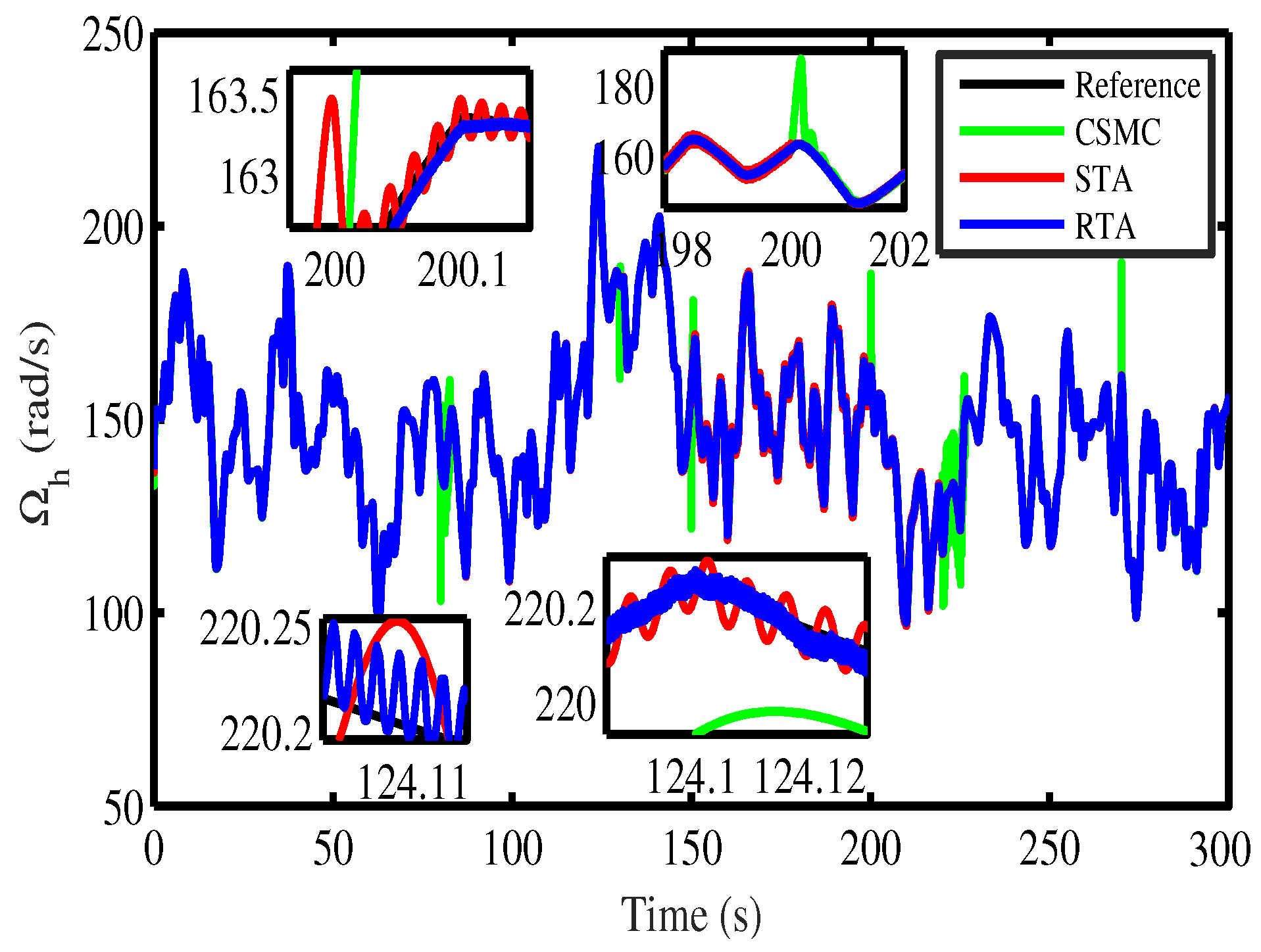
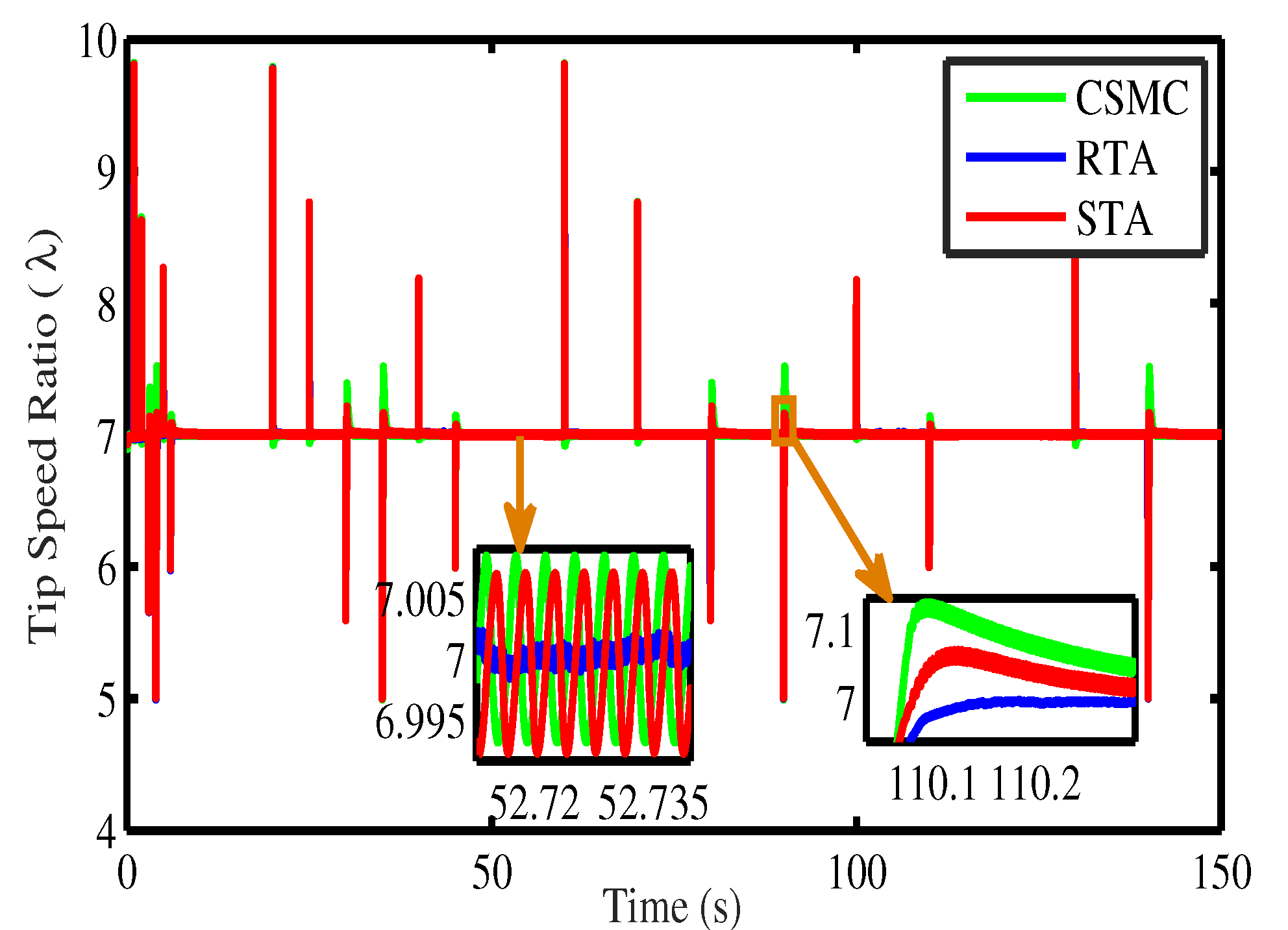
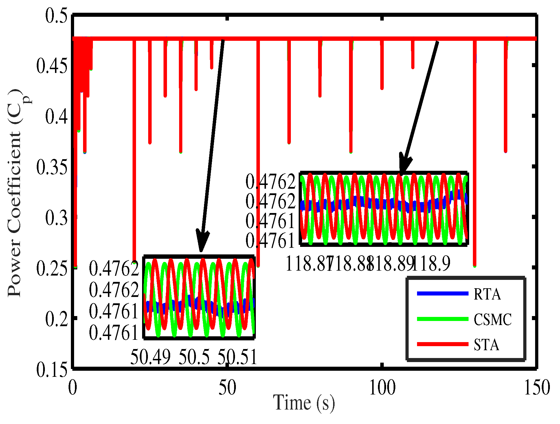
In the nominal case, the wind turbine is operated at optimum TSR (${\lambda }_{opt}$) that will confirm $C_{pmax}$. The three algorithms CSMC, STA, and RTA are then employed to enable maximum power extraction. This is accomplished by controlling the rotational speed of PMSG at optimum values. The algorithms confirm the tracking of HSS rotational speed (Figure 7) while keeping the tip speed ratio at its optimum value (Figure 8) and the coefficient of power at $C_{pmax}=0.476$ (Figure 9). In Figure 7, it is worth noticing that the CSMC offers poor tracking performance and pronounced chattering effects. The STA, which is sensitive to un-modeled fast dynamics, offers relatively good tracking performance but exhibits some chattering as well. In the case of the proposed algorithm, the elimination of chattering and superior tracking performance is evident. In addition, the tip speed ratio ($\lambda$), power coefficient ($C_p$), mechanical torque (${\mathsf{\Gamma }}_m$), andthe mechanical power on generator side ($P_{m_{HSS}}$) against TSR ($\lambda$), shown in Figure 8, Figure 9, Figure 10 and Figure 11, respectively, further confirm the efficacy of the proposed RTA-based algorithm. In Figure 10 and Figure 11, it can be observed that the RTA reaches the manifold smoothly despite all the nonlinearities and stays there with minimal/negligible amplitude of chattering, the STA undergoes a slightly longer transient phase (known as the reaching phase in the sliding mode control theory), while the CSMC exhibits chattering, a noticeable reaching phase, and poor performance in the sliding phase. Thus, MPPT is more effective in the case of the proposed RTA.

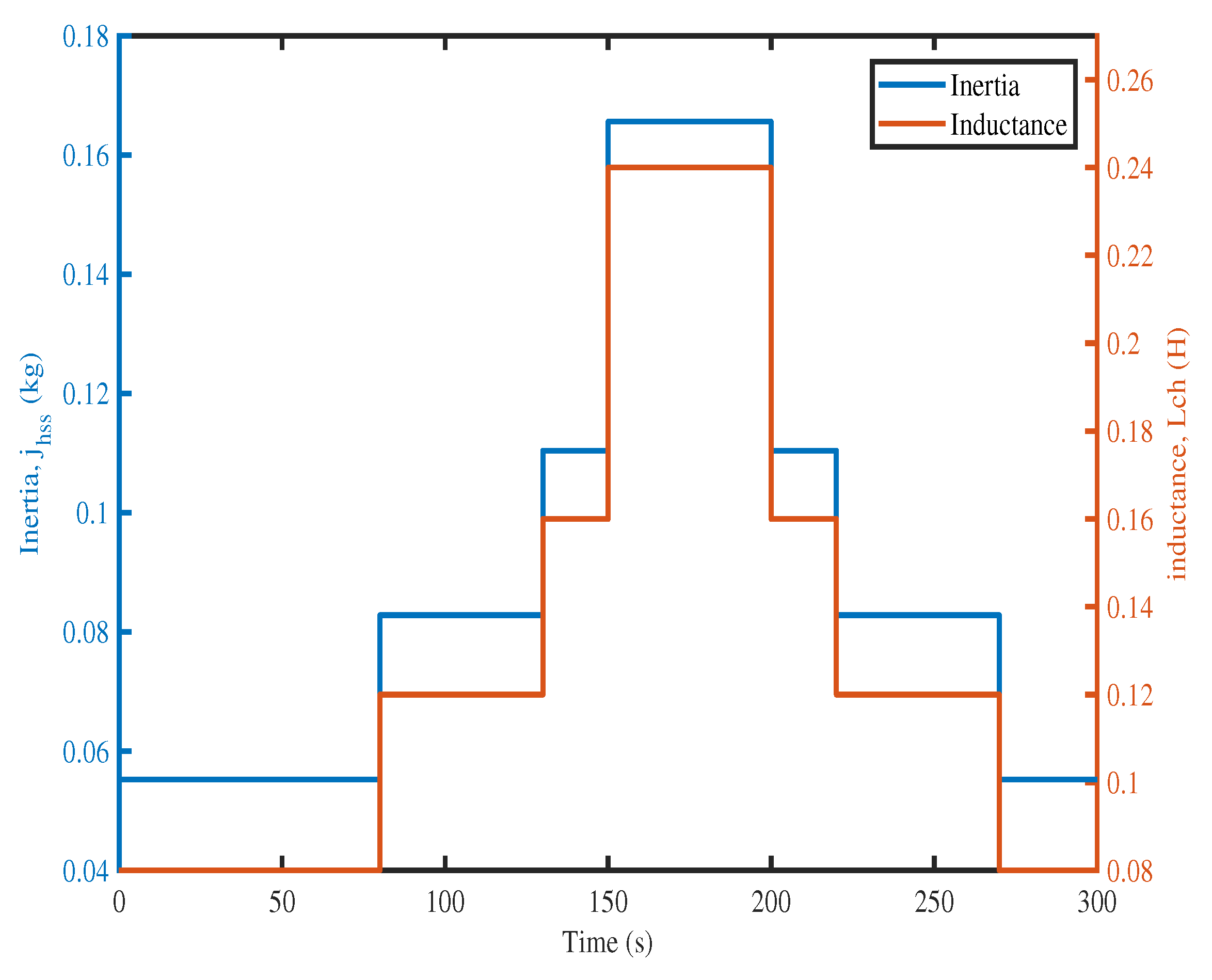
7.2. Varying Load and Varying Inertia

The robustness of the proposed algorithm is demonstrated in the presence of varying load inductance and inertia profiles, as shown in Figure 12.

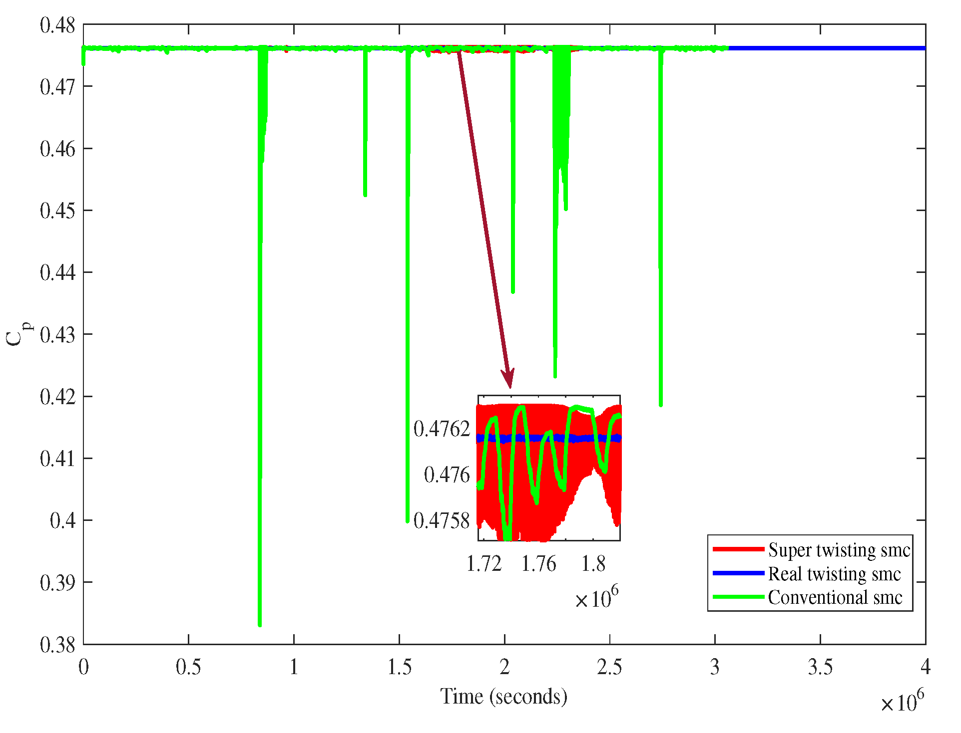
At the instances of transition in load inductance/inertia (see Figure 12), the proposed RTA algorithm outperforms the STA and CSMC while tracking the HSS side angular speed as shown in Figure 13. The zoomed portions indicate the transition instances of the load/inertia where the STA and CSMC exhibit oscillatory behavior which can cause lower power extraction. This distraction at the transition instances of STA and CSMC is more evident in the tip speed ratio and power coefficient shown in Figure 14 and Figure 15, respectively. In Figure 15, the $C_p$ goes to a very low value, about 38% for CSMC, while the RTA retains $C_p$ to its optimum which ensures its robustness again parametric variations and also provides MPP.

7.3. Varying Wind Speed

The system is now subjected to sharp variations in wind speed in order to further elaborate the robust performance of the proposed algorithm. In such a scenario, it is desirable that the system should operate at $C_{p_{max}}$.

In Figure 16, it is worth mentioning that the variations in wind speed cause the CSMC and STA to exhibit almost a transient behavior at each instant of time while the RTA provides smooth tracking of angular speed at HSS. Although some transient distractions can be observed in tip-speed and power coefficient, they do not have remarkable effects on the control scheme performance and system stability as shown in Figure 17 and Figure 18, respectively. These results demonstrate that the proposed algorithm offers robust performance and thus maintains the MPPT along with minimized chattering.

8. Conclusions

In this work, the model of a PMSG-based WECS is presented with three states, and then it is transformed to a two states normal form with the output-oriented model. The normal form states are then equipped with SMC (CSMC, STA, and RTA) for the tracking of wind speed in three cases, i.e., the nominal case, varying load and varying inertia case, and finally the deterministic case of wind speed profile for the robustness evaluation of the controllers. In a practical environment, one may not be available with nonlinear terms and aerodynamic forces, hence, an offline NeuroFuzzy scheme is designed for the estimation of nonlinear drift (i.e., $L_f^{2}h\left(x\right)and{L}_g{L}_{f}h\left(x\right)$). Meanwhile, the rotational speed of the PMSG rotor was available, therefore, the missing derivative of HSS has been estimated via the URED. During the simulation process, it was observed that the CSMC was showing oscillatory behavior (chattering) with a considerable steady-state error, which was further improved via a replacement of the discontinuous control component with the STA and RTA. The simulation results in the presence of varying load varying inertia disturbances and abrupt variations in wind speed are quite delightful and the newly examined law showed to be a more practical and appealing candidate for an MPPT. In nutshell, this new law outshines all the employed designed strategies.

References

- Baroudi, J.A.; Dinavahi, V.; Knight, A.M. A review of power converter topologies for wind generators. Renew. Energy 2007, 32, 2369–2385. [Google Scholar] [CrossRef]
- Housseini, B.; Okou, A.F.; Beguenane, R. Performance comparison of variable speed PMSG-based wind energy conversion system control algorithms. In Proceedings of the Ecological Vehicles and Renewable Energies (EVER), 2017 Twelfth International Conference on. IEEE, Monte Carlo, Monaco, 11–13 April 2017; pp. 1–10. [Google Scholar]
- Yaramasu, V.; Dekka, A.; Durán, M.J.; Kouro, S.; Wu, B. PMSG-based wind energy conversion systems: Survey on power converters and controls. IET Electr. Power Appl. 2017, 11, 956–968. [Google Scholar] [CrossRef]
- Kumar, D.; Chatterjee, K. A review of conventional and advanced MPPT algorithms for wind energy systems. Renew. Sustain. Energy Rev. 2016, 55, 957–970. [Google Scholar] [CrossRef]
- Dalala, Z.M.; Zahid, Z.U.; Yu, W.; Cho, Y.; Lai, J.S.J. Design and analysis of an MPPT technique for small-scale wind energy conversion systems. IEEE Trans. Energy Convers. 2013, 28, 756–767. [Google Scholar] [CrossRef]
- De Kooning, J.D.; Gevaert, L.; Van de Vyver, J.; Vandoorn, T.L.; Vandevelde, L. Online estimation of the power coefficient versus tip-speed ratio curve of wind turbines. In Proceedings of the Industrial Electronics Society, IECON 2013-39th Annual Conference of the IEEE, Vienna, Austria, 10–13 November 2013; pp. 1792–1797. [Google Scholar]
- Abdullah, M.; Yatim, A.; Tan, C. An online optimum-relation-based maximum power point tracking algorithm for wind energy conversion system. In Proceedings of the Power Engineering Conference (AUPEC), 2014 Australasian Universities, Perth, WA, Australia, 28 September–1 October 2014; pp. 1–6. [Google Scholar]
- Thongam, J.S.; Ouhrouche, M. MPPT control methods in wind energy conversion systems. In Fundamental and Advanced Topics in Wind Power; InTech: Houston, TX, USA, 2011. [Google Scholar]
- Kazmi, S.M.R.; Goto, H.; Guo, H.J.; Ichinokura, O. A novel algorithm for fast and efficient speed-sensorless maximum power point tracking in wind energy conversion systems. IEEE Trans. Ind. Electron. 2011, 58, 29–36. [Google Scholar] [CrossRef]
- Bendib, B.; Belmili, H.; Krim, F. A survey of the most used MPPT methods: Conventional and advanced algorithms applied for photovoltaic systems. Renew. Sustain. Energy Rev. 2015, 45, 637–648. [Google Scholar] [CrossRef]
- Calderaro, V.; Galdi, V.; Piccolo, A.; Siano, P. A fuzzy controller for maximum energy extraction from variable speed wind power generation systems. Electr. Power Syst. Res. 2008, 78, 1109–1118. [Google Scholar] [CrossRef]
- Soufi, Y.; Kahla, S.; Bechouat, M. Feedback linearization control based particle swarm optimization for maximum power point tracking of wind turbine equipped by PMSG connected to the grid. Int. J. Hydrog. Energy 2016, 41, 20950–20955. [Google Scholar] [CrossRef]
- Di Piazza, A.; Di Piazza, M.C.; Vitale, G. Solar and wind forecasting by NARX neural networks. Renew. Energy Environ. Sustain. 2016, 1, 39. [Google Scholar] [CrossRef]
- Di Piazza, A.; Di Piazza, M.C.; La Tona, G.; Luna, M. An artificial neural network-based forecasting model of energy-related time series for electrical grid management. Math. Comput. Simul. 2021, 184, 294–305. [Google Scholar] [CrossRef]
- Meharrar, A.; Tioursi, M.; Hatti, M.; Stambouli, A.B. A variable speed wind generator maximum power tracking based on adaptative neuro-fuzzy inference system. Expert Syst. Appl. 2011, 38, 7659–7664. [Google Scholar] [CrossRef]
- Sebaaly, F.; Vahedi, H.; Kanaan, H.; Moubayed, N.; Al-Haddad, K. Sliding-mode current control design for a grid-connected three-level NPC inverter. In Proceedings of the International Conference on Renewable Energies for Developing Countries 2014, Beirut, Lebanon, 26–27 November 2014; pp. 217–222. [Google Scholar]
- Khan, I.; Bhatti, A.I.; Arshad, A.; Khan, Q. Robustness and performance parameterization of smooth second order sliding mode control. Int. J. Control. Autom. Syst. 2016, 14, 681–690. [Google Scholar] [CrossRef]
- Kazmi, S.M.R.; Goto, H.; Guo, H.J.; Ichinokura, O. Review and critical analysis of the research papers published till date on maximum power point tracking in wind energy conversion system. In Proceedings of the Energy Conversion Congress and Exposition (ECCE), 2010 IEEE, Atlanta, GA, USA, 12–16 September 2010; pp. 4075–4082. [Google Scholar]
- Khan, I. On Performance Based Design Of Smooth Sliding Mode Control. Ph.D. Thesis, Capital University of Science & Technology Islamabad, Islamabad, Pakistan, 2016. [Google Scholar]
- Meghni, B.; Dib, D.; Azar, A.T. A second-order sliding mode and fuzzy logic control to optimal energy management in wind turbine with battery storage. Neural Comput. Appl. 2017, 28, 1417–1434. [Google Scholar] [CrossRef]
- Butt, Q.R.; Bhatti, A.I. Estimation of gasoline-engine parameters using higher order sliding mode. IEEE Trans. Ind. Electron. 2008, 55, 3891–3898. [Google Scholar] [CrossRef]
- Eghtesad, M.; Bazargan-Lari, Y.; Assadsangabi, B. Stability analysis and internal dynamics of MIMO GMAW process. IFAC Proc. Vol. 2008, 41, 14834–14839. [Google Scholar] [CrossRef]
- Cruz-Zavala, E.; Moreno, J.A.; Fridman, L.M. Uniform robust exact differentiator. IEEE Trans. Autom. Control. 2011, 56, 2727–2733. [Google Scholar] [CrossRef]
- Rafiq, M. Higher Order Sliding Mode Control Based Sr Motor Control System Design. Ph.D Thesis, Mohammad Ali Jinnah University Islamabad, Islamabad, Pakistan, 2012. [Google Scholar]
- Levant, A. Sliding order and sliding accuracy in sliding mode control. Int. J. Control 1993, 58, 1247–1263. [Google Scholar] [CrossRef]
Figure 1.
Schematic of the designed WECS.
Figure 2.
Turbine speed versus turbine power for different wind speeds.
Figure 3.
MISO adaptive NeuroFuzzy network structure for the estimation of and .
Figure 4.
Closed-loop observer-based SMC PMSG-WECS configuration.
Figure 5.
tracking in the nominal case.
Figure 6.
tracking in the varying load and varying inertia case.
Figure 7.
The reference and actual PMSG side-shaft speed.
Figure 8.
Tip speed ratios.
Figure 9.
Turbine power coefficients.
Figure 10.
Electromagnetic torque versus tip speed ratio.
Figure 11.
High-speed shaft side power versus tip speed ratio.
Figure 12.
Varying load, varying inertia.
Figure 13.
PMSG side-shaft speed.
Figure 14.
Tip speed ratio.
Figure 15.
Power coefficients.
Figure 16.
PMSG side angular speed.
Figure 17.
Figure 18.