
Identification of Breakpoints in Carbon Market Based on Probability Density Recurrence Network
by
 , and
, and
Mengrui Zhu
1, 
Hua Xu
2,*,
Xingyu Gao
3,
Minggang Wang
1,2,4,
André L. M. Vilela
5,6 and
Lixin Tian
1,4
1
School of Mathematical Science, Nanjing Normal University, Nanjing 210042, China
2
Department of Mathematics, Nanjing Normal University Taizhou College, Taizhou 225300, China
3
School of Mathematics and Statistics, Changshu Institute of Technology, Changshu 215500, China
4
School of Mathematical Science, Jiangsu University, Zhenjiang 212000, China
5
Center for Polymer Studies and Department of Physics, Boston University, Boston, MA 02115, USA
6
Física de Materiais, Universidade de Pernambuco, Recife 50100-010, Pernambuco, Brazil
*
Author to whom correspondence should be addressed.
Energies 2022, 15(15), 5540; https://doi.org/10.3390/en15155540
Submission received: 14 July 2022
/
Revised: 25 July 2022
/
Accepted: 27 July 2022
/
Published: 30 July 2022
(This article belongs to the Special Issue Modeling and Analysis of Energy Systems and Sustainable Energy Transition)
Abstract
:The scientific judgement of the structural abrupt transition characteristics of the carbon market price is an important means to comprehensively analyze its fluctuation law and effectively prevent carbon market risks. However, the existing methods for identifying structural changes of the carbon market based on carbon price data mostly regard the carbon price series as a deterministic time series and pay less attention to the uncertainty implied by the carbon price series. We propose a framework for identifying abrupt transitions in the carbon market from the perspective of a complex network by considering the influence of random factors on the carbon price series, expressing the carbon price series as a sequence of probability density functions, using the distribution of probability density to reveal the uncertainty information implied by carbon price series and constructing a recurrence network of carbon price probability density. Based on the community structure, the break index and statistical test method are defined. The simulation verifies the effectiveness and superiority of the method compared with traditional methods. An empirical analysis uses the carbon price data of the European Union carbon market and seven pilot carbon markets in China. The results show many abrupt transitions in the carbon price series of the two markets, whose occurrence period is closely related to major events.
1. Introduction
Countries around the world have taken measures to control greenhouse gas emissions. The carbon emission trading mechanism optimizes the allocation of carbon emission space resources through market mechanisms. Since the Kyoto Protocol came into effect, the international carbon market has shown a rapid growth trend. At present, twenty-seven jurisdictions of different levels in the world (one supranational institution, four countries, fifteen provinces/states, and seven cities) have instituted carbon emission trading mechanisms, accounting for 8% of total global carbon emissions. The European Union Emission Trading Mechanism (EU ETS) is relatively complete and is the most influential. The mechanism covers more than 10,000 emitters from the EU member countries in power, combustion devices, oil refining, steel, cement, glass, lime, ceramics, paper making, and other industries, accounting for more than 40% of the total EU greenhouse gas emissions. The EU ETS is constantly improved. China is one of the largest emitters of greenhouse gases. At the 2020 Climate Ambition Summit, China promised to strive for peak carbon dioxide emissions by 2030 and carbon neutrality by 2060. China has established a national carbon market to support its energy transformation and realize green and low-carbon development. However, there are problems, such as an imperfect operation mechanism and insufficient market vitality [1,2].
The carbon price is the core index of the carbon market. For various reasons, the carbon price fluctuates greatly under different economic backgrounds [3,4]. The breakpoint in the EU ETS may affect the data generation process of the European Union Allowance (EUA) price, and then, the allowance management and policy formulation. Therefore, it is of great significance to identify the breakpoints in the carbon price. Perron (1989) proposed a direct breakpoint test [5]. Zivot (1992), Lumsdaine and Papell (1997), and Lee et al. (2004) [6,7,8] improved these methods using the in-model biochemistry, but these methods can only be used to detect breakpoints twice, at most. Bai and Perron (2003) [9] studied a linear regression model with multiple structural changes and proposed a multiple mean structural change test method. Lin et al. (2007) [10] pointed out that the spot price of carbon dioxide follows a mean regression process. Alberola, Chevallier, and Chèze (2008) [11] detected structural price changes in April and October of 2006 in the first stage of the EU ETS. Benz and Trück (2009) [12] used the Markov regime-switching and ARCH–GARCH models to analyze the short-term spot price dynamics of the EUA. Daskalakis et al. (2009) [13] modeled the random behavior of the European carbon dioxide spot price using the jump-diffusion technology and found that it may have the characteristics of jump and non-stationarity. Vallier (2011) [14] studied the instability in carbon prices during 2005–2008 based on retrospective [9,15,16,17] and forward-looking tests [18,19]. Conrad et al. (2012) [20] modeled the price adjustment process of the EUA and found that fractionally integrated asymmetric power GARCH can well capture high-frequency EUA price dynamics. Wu et al. (2015) [21] used the Bai–Perron method to test the number of structural changes and corresponding time-varying points of the EUA price. Zhu et al. (2015) [22] detected three breakpoints in the EU ETS from 2005 to 2012 based on an iterative cumulative sum of squares algorithm and event research model and found their time of occurrence to be closely related to historical events, such as the global financial crisis and the European debt crisis. Jia et al. (2019) [23] identified the breakpoints of the EU ETS in 2005–2018 using a multiple structural change model and explained their impact on the expected carbon returns and volatility using bilaterally modified dummies. Yang et al. (2020) [24] quantitatively analyzed the effectiveness of the carbon market using a Hurst index based on market structure breakpoints and found that the EU ETS had more structural breakpoints than the Hubei and Shanghai pilot markets, and these were more susceptible to external factors. Li et al. (2020) [25] selected the carbon trading week data of seven pilot markets from 14 May 2014 to 25 April 2018 and found, using the Bai–Perron structural change method, that there was one breakpoint in Guangdong and Hubei and two in Tianjin. Dong et al. (2022) [26] used the Bai–Perron structural break test to analyze the factors that affect the price fluctuation of EU carbon allowance futures. The research shows that the outbreak of COVID-19 and the “EUR 750 billion green recovery plan “ have both had a significant impact on the EU carbon price, resulting in a significant structural change in the carbon price. Using time-series data from 1986 to 2019 and environmental degradation being measured by CO2 emissions, Nguygn et al. (2021) [27] studied the influence of some factors on environmental degradation using the structural break unit root test. Zheng et al. (2021) [28] tested the effects of oil shocks on the returns of the European Union’s carbon emission allowance (EUA) under different market conditions by using a quantile regression method and looked into whether the link between the oil shocks and the returns of the EUA has any asymmetry or lagged effects. Zahoor et al. (2022) [29] used the structural break unit root test and the robust least square regression method to prove that clean energy investment is negatively correlated with carbon dioxide emissions and positively correlated with China’s economic growth. For the sharp rise and fall of stock prices, Yang et al. (2022) [30] used the heuristic segmentation algorithm of nonlinear time series mutation detection to study the detection of market dynamics characteristics before the stock market crash.
Research on the carbon market has many limitations. At present, econometric models are mostly used to identify structural changes in carbon markets based on carbon price data, and the existing methods seldom consider the uncertainty implied by the carbon price series [31,32]. With the development of complex network tools, more and more attention has been paid to the uncertainty of carbon price fluctuations by using complex network methods [33,34,35,36]. This paper proposes a framework to identify abrupt transitions in the carbon market, considering random factors, expressing the carbon price series as probability density functions, constructing a probability density recurrence network (PDRN), and identifying breakpoints in the carbon market based on the community structure of the network. Our work has the following features and innovations: (1) taking the probability distribution function sequence corresponding to the carbon price sequence as the research object, a PDRN construction method of the carbon price is proposed; (2) based on the community structure of the PDRN of the carbon price, an index to measure its structural change is proposed, and a statistical test method for the calculation results of the index is designed; (3) based on the price data of the EU carbon market and seven pilot carbon markets in China, their breakpoints in different periods are calculated, and their structural abrupt change characteristics are compared and analyzed.
The rest of this paper is organized as follows. Section 2 presents our methodology. Section 3 verifies the effectiveness and superiority of our method by simulation. Section 4 and Section 5 empirically analyze the carbon price data of the EU ETS and the China carbon market, respectively. Section 6 is a summary of this paper with a brief conclusion.
2. Preliminaries and Proposed Method
2.1. Preliminaries
2.1.1. Bai–Perron Test
Assuming that there are two breakpoints in the sequence as an example, the Bai–Perron test model is as follows [37]:
where is the dummy variable matrix of order , and is the corresponding coefficient matrix. For every two sudden change time points to be selected, there are three models, and the coefficient matrix of each model corresponding to the dummy variables is , , and . There are two dummy variables and two breakpoints. Therefore, among the models with two breakpoints extracted from all sample points, the residual of the model after determining the coefficients by OLS is calculated, and then, the residual of three models with different break change times is horizontally compared, and finally, the break time point that minimizes the residual of the model when there is one, two, and no structural mutation is determined. When it is extended to the case of breakpoints, the models are selected to determine the structural breakpoint that is most likely to have mutation under a different number of breakpoints.
2.1.2. Recurrence Network
The recurrence plot can be represented by a matrix in the form of [34]
where represents the number of observation points, is the recurrence threshold, ‖·‖ can be any norm in the phase space (for example, the Manhattan norm, Euclidean norm, or infinite norm), and is a function ( when , otherwise ). That is, when and are sufficiently close (i.e., ), it is considered that node and node are connected by undirected edge; otherwise, there is no link between node and node . The adjacency matrix of the network is defined as
where represents the identity matrix. The elements on the main diagonal of the adjacent matrix are all , and the other elements in the matrix are symmetrical toward the main diagonal. Therefore, the traditional recurrence network is a simple, powerless and undirected network without self-loop.
2.2. The Proposed Method
We propose a framework based on a PDRN to identify breakpoints in a time series considering the influence of random factors. We transform the obtained time series data to a probability density function (PDF) sequence that describes the distribution characteristics of the probability of time series data at a certain time point; hence, the uncertain features of the original time series data can be captured. We propose an index to identify the breakpoints of the time series and a framework for statistical tests.
2.2.1. Probability Density Recurrence Network
Let the random variables corresponding to the observable and at time and be and , respectively, and define as the random variables, which describe the difference between and . Then, the probability of recurrence under the threshold can be expressed as
where |·| denotes the absolute value. Equation (4) can be written as
where is the joint probability density function. According to the relationship between the density and distribution functions, can be regarded as the probability that falls in the interval , and we can write Equation (5) as
which implies
where , and is the cumulative distribution function (CDF) of .
The upper-bound and lower-bound for the cumulative distribution function can be estimated by the results from the literature [38] as
where . Then, we can ensure that . Hence, the upper-bound and lower-bound for can be written as
Given a recurrence threshold , we can deduce that .
We assume that the probability is a random variable distributed in the interval and define its probability density as . Then, we write the connection probability of the time series between and as
where is the probability that , given . Equation (10) shows that the probability of links between the nodes can be calculated using the expectation of . Suppose uniformly distributed in the interval , the probability is
To sum up, we can obtain the adjacency matrix of the system’s PDRN as
2.2.2. Definition of Break Index and Statistical Test Based on Community Structure
The dynamic change of community structure in a recurrence network can be used to reveal the occurrence of an abrupt transition [39]. Hence, we divide the time series into several equal small-scale periods (windows) and construct a PDRN in each time window. We consider the sliding window at time , which covers the time period , and define . Based on the changes of the network community structure around time , we define an index to detect an abrupt transition:
where is an adjacency matrix covering the interval . From the changes of with time, we can detect the occurrence of an abrupt transition. To test that the abrupt transitions of the two halves of the network (before and after the midpoint) are real dynamic transitions and not due to chance, we carry out a statistical test, making the following assumption.
Null hypothesis: obeys a uniform distribution in the interval .
To test whether the null hypothesis is correct, we calculate the -value corresponding to in different time windows. We first calculate corresponding to the PDRN constructed in each time window and define it as . Secondly, we calculate the degree sequence of the PDRN, simulate random networks with this degree sequence (for accuracy, should be as large as possible), and calculate corresponding to each random network. Then, we can obtain the set of of the random network. Therefore, we can estimate the values of corresponding to as
where is the percentile function. Suppose the confidence level is set to . If , we can reject the original hypothesis, i.e., the change of network structure is not caused by randomness but by the real dynamic transition of the system.
2.2.3. Method to Identify Breakpoints in Carbon Market Based on PDRN
To identify breakpoints of the carbon market based on the construction of a PDRN of the carbon price, we consider whether the carbon price data are one dimensional or high dimensional.
Method to Identify Breakpoints of One-Dimensional Carbon Price Data
For a one-dimensional carbon price data series, we identify breakpoints based on the PDRN, as follows.
Step 1: Construct sliding windows. Let the data series of the carbon price be . Set the length of the sliding window as , and set the sliding step as (generally, ). Then, we obtain small-scale sliding windows. Therefore, we can obtain an -dimensional data matrix , , .
Step 2: Construct a PDRN. For data matrix , set the length of the sliding window as , and set the sliding step as (generally, ). Then, we can obtain sliding windows. Within each sliding window, the kernel density of each column of data is estimated, and the probability density sequence is obtained. Based on that, the PDRN sequence is obtained by applying the method in Section 2.1.
Step 3: Calculate the break index. In each time window, the abrupt transition index is calculated using Equation (13).
Step 4: Conduct statistical tests. We construct the random network in each time window and calculate the probability corresponding to the break index using Equation (14).
Method to Identify Breakpoints of High-Dimensional Carbon Price Data
For high-dimensional carbon price data, we can identify breakpoints using steps 2–4 above. In particular, if the collected carbon price data are two dimensional, such as the highest daily value and the lowest daily value , we can assume that the carbon price is uniformly distributed in the interval . Then, we can obtain the sequence of PDFs:
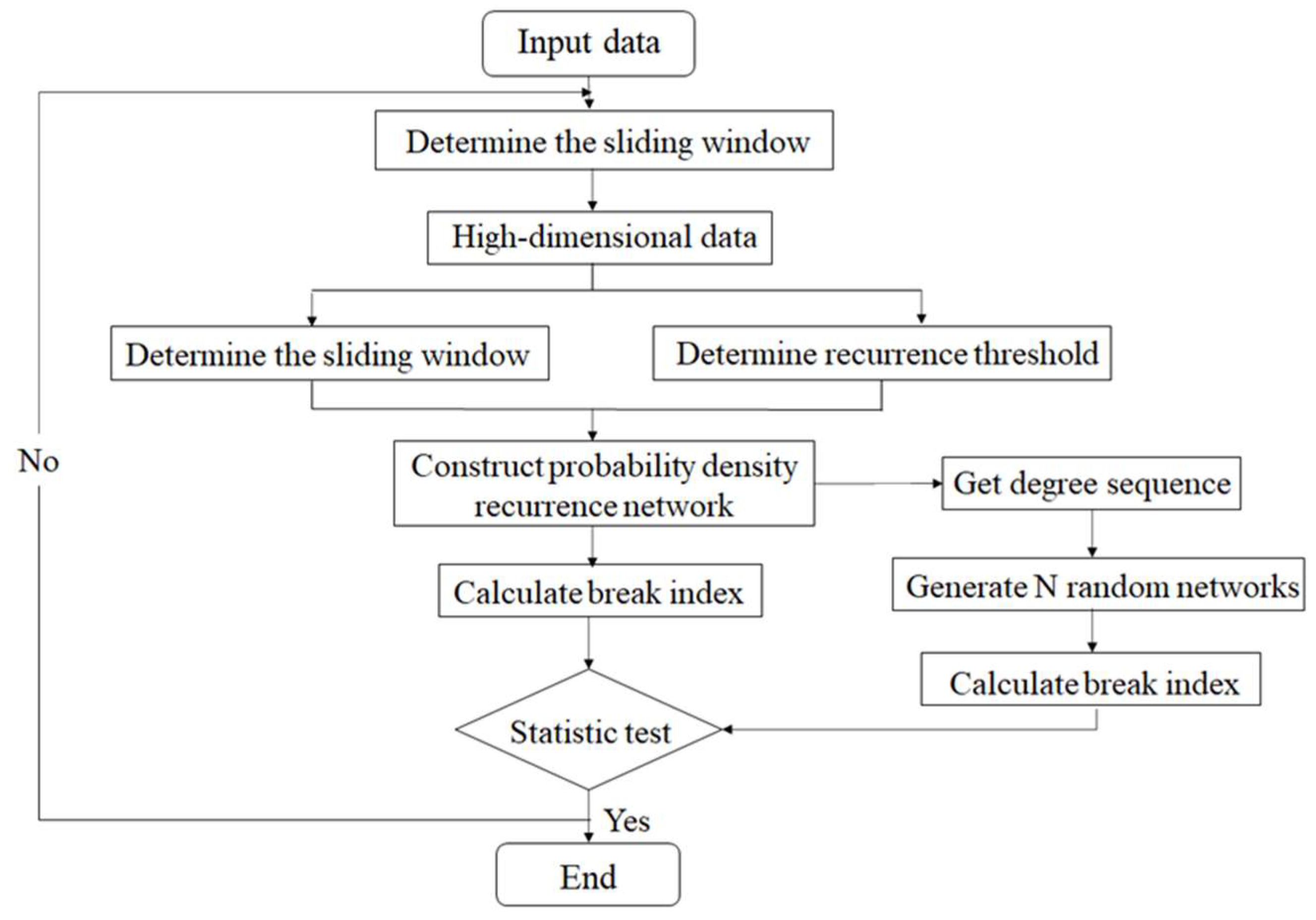
Furthermore, we can construct the PDRN and identify the breakpoints based on steps 3–4 above. In the empirical analysis of this paper, we will analyze the results of identifying the breakpoints in the carbon market. The flowchart of the algorithm is shown in Figure 1.
As can be seen from Figure 1, for the given carbon price data, we first convert them into high-dimensional data by setting a sliding window, then construct a probability density recurrence network and calculate its break index, and then obtain the initial breakpoints, generate a random network with the same degree sequence as the PDRN, and calculate its break index. Finally, we conduct the statistic test according to Equation (14). The points that fail the test are pseudo-breakpoints, and those that pass the test are the real breakpoints that we finally obtain.
3. Numerical Simulation
To verify that the proposed method can identify breakpoints in a time series, we construct a dataset:
where , and is Gaussian white noise. At each location , we impose the following transitions:
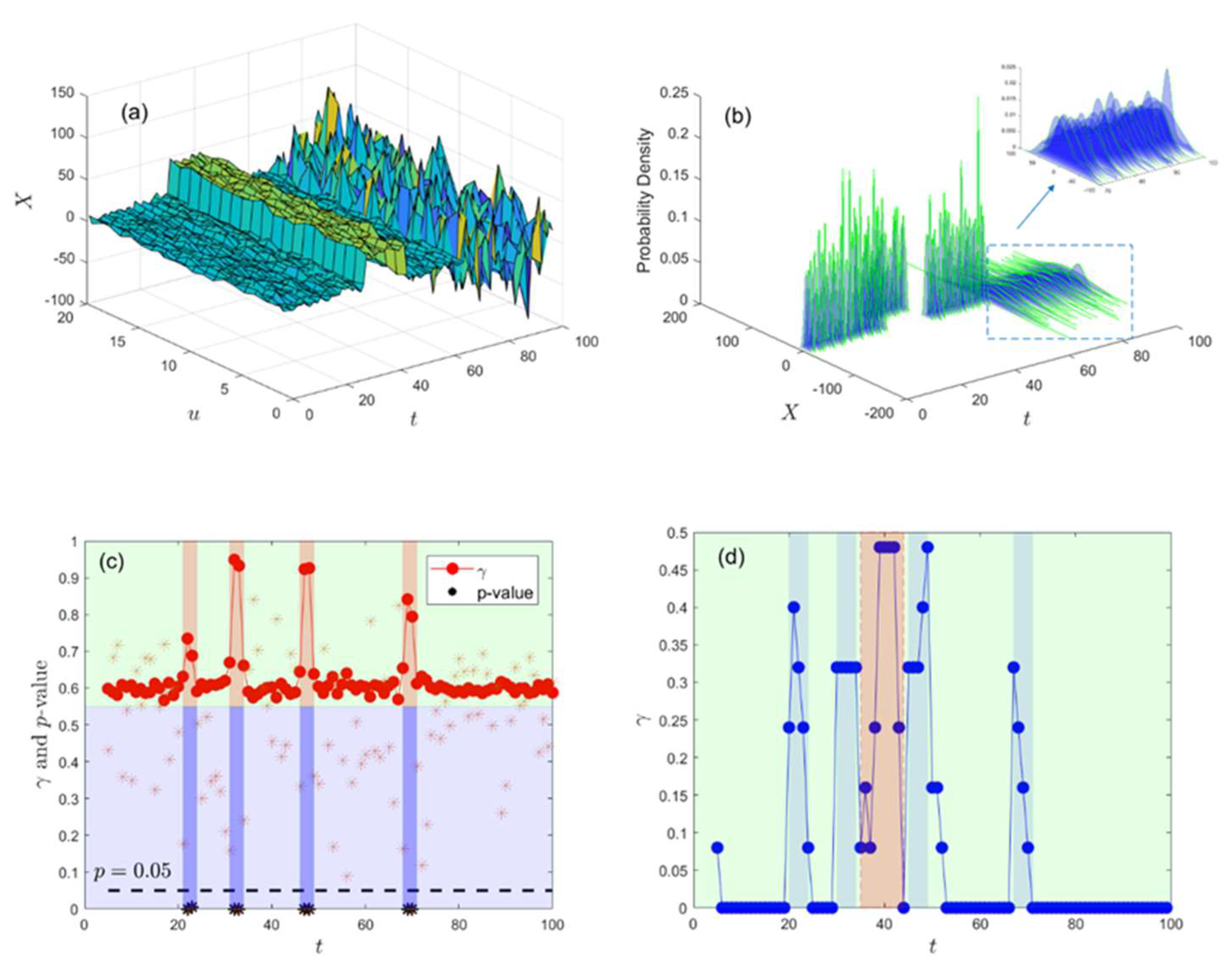
To simulate noisy measurements, our time series is , whose evolution and probability density images are obtained by drawing with MATLAB, as shown in Figure 2a,b. We set and the sliding step to , thus obtaining time windows. In each time window, the threshold . We construct the PDRN and calculate the break index and probability using Equations (13) and (14), respectively, as shown in Figure 2c. To illustrate the superiority of the method proposed in this paper, the evolution of with time based on a traditional recurrence network is shown in Figure 2d.
The numerical simulation data in Figure 2a suddenly change at , and . Using the proposed method to calculate , four breakpoints can be observed (Figure 2c), with -values less than 0.05, which shows that the decision to reject the original hypothesis can be made at a confidence level , and the four detected breakpoints are real. Correspondingly, through the detection of the traditional recurrence network (Figure 2d), we can find that the values of in the intervals of are all large, and the real breakpoints cannot be accurately identified because the simulated data contain noise interference, to which the traditional recurrence network method is susceptible. This also shows that the proposed method has advantages in terms of anti-noise interference and accurate identification of system breakpoints.
4. Empirical Analysis of Breakpoints Identification in EU ETS
We empirically analyze the price data of the EU carbon market, selecting the daily closing price from 2 January 2013 to 30 September 2020 and using the highest and lowest prices as sample data to identify breakpoints. Table 1 presents the descriptive statistical results of the sample data. It can be seen that the means of the daily closing price, highest price, and lowest price are all around 11.5, and the data fluctuate greatly. The skewness of these price series is greater than zero, which obeys the right distribution, and the kurtosis is slightly less than 3, which indicates that the distribution density curve is smoother than the normal distribution near its peak value. The results of the Jarque–Bera test show that the null hypothesis is rejected at the 1% significance level, i.e., the sample data do not conform to a normal distribution. From the results of the ADF test, the t-values of the closing price, highest price, and lowest price are all greater than the critical value at the 1% significance level. Accepting the original hypothesis, there are unit roots in these time series, i.e., the sample data series is nonstationary.
4.1. Identification of Breakpoints of Carbon Price in the EU ETS Based on Daily Highest–Lowest Prices
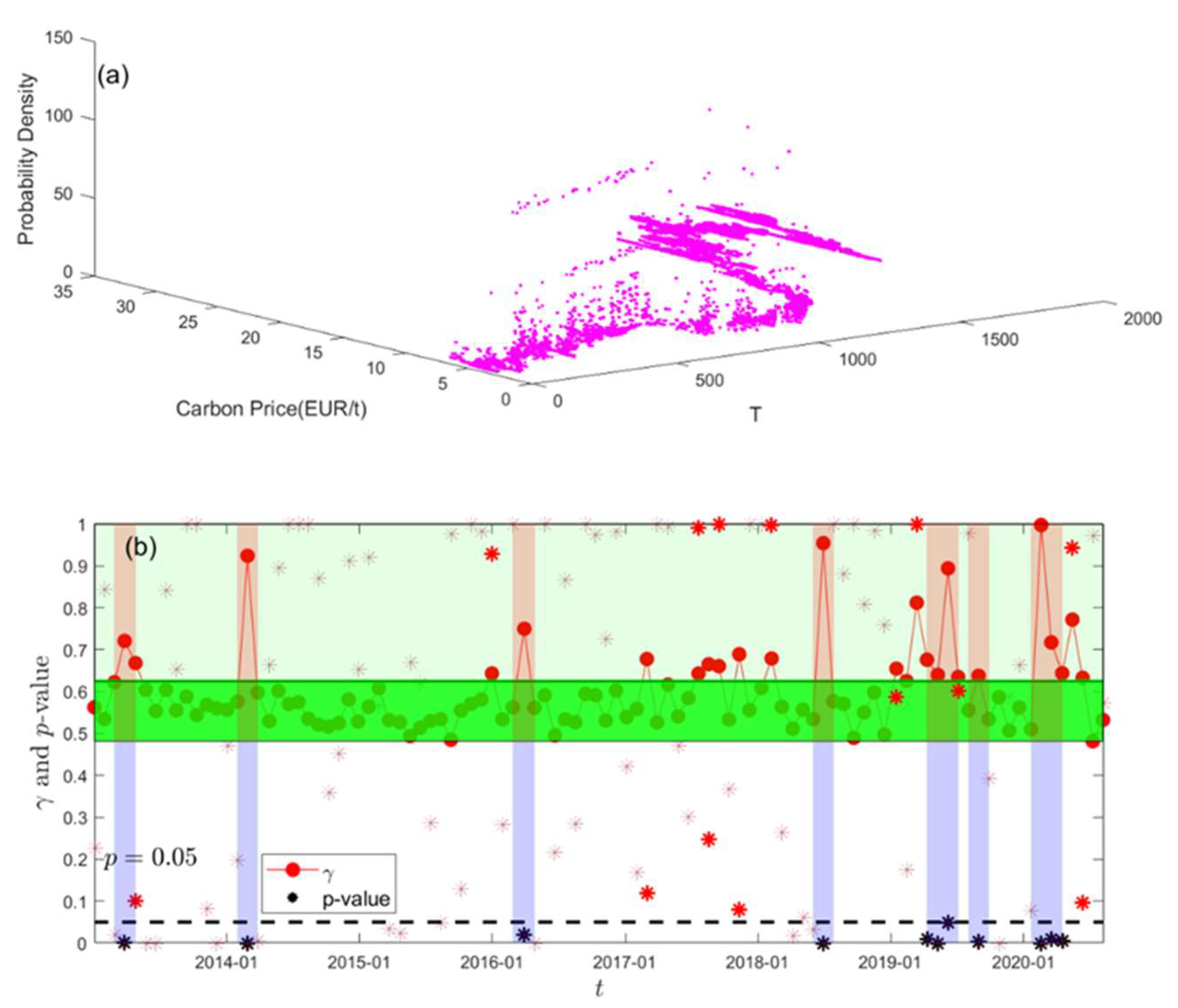
We select the highest and lowest daily prices in the EU ETS as sample data to identify the breakpoint of the carbon market price. We assume that it follows a uniform distribution between the lowest and highest prices and use Equation (15) to obtain the probability density image of the selected sample data, as shown in Figure 3a. With and , we obtain time windows. With the recurrence threshold in each time window, we calculate the break index and the corresponding -value using Equations (13) and (14), respectively, as shown in Figure 3b.
As can be seen from Figure 3b, there are 24 break indices whose values are greater than the 75% quantile of the break index dataset, 13 with . Based on the judgment criterion of breakpoint identification (with both a large break index and a small probability ), the time points corresponding to these 13 break indices cannot be judged as breakpoints of the EU ETS. The -values of the other 11 break indices are all less than 0.05, which are distributed over six periods, indicating a structural change in the carbon price of the EU ETS in these periods. One breakpoint is detected in March 2013, with break index and . One is detected in March 2014, with break index and ; one in March 2016, with break index and ; and one in June 2018, with break index and . Four breakpoints are detected from April to August 2019, with break indices of , respectively, and respective -values of . Three breakpoints are detected from April to May 2020, with break indices of , respectively, and respective -values of .
4.2. Identification of Breakpoints of Carbon Price in the EU ETS Based on Daily Closing Price
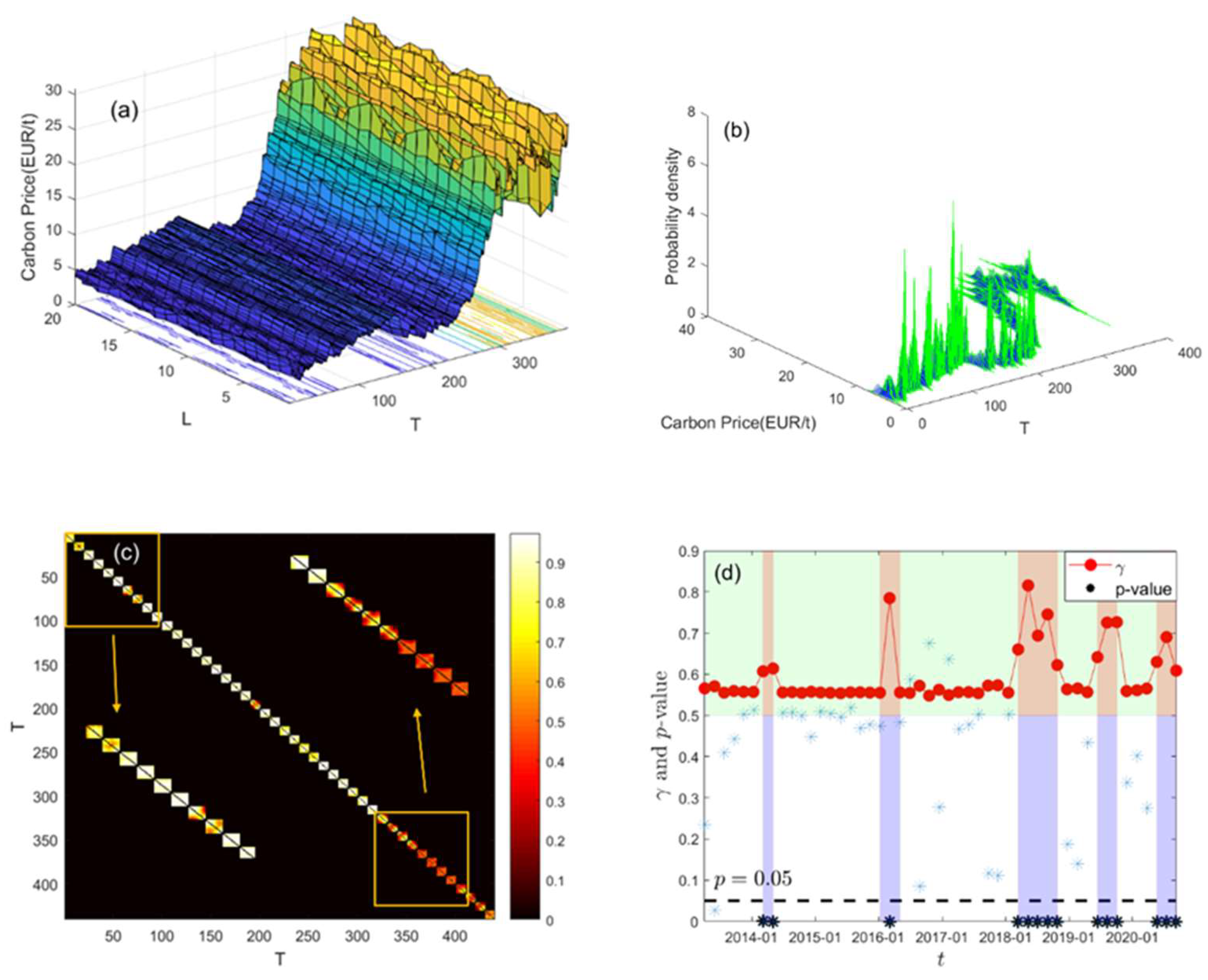
To construct a PDRN for the one-dimensional closing price data of the EU carbon market, we transform it to high-dimensional data by constructing sliding windows, with sliding window length and sliding step , to obtain time windows with carbon price data with dimension . Figure 4a shows the evolution image of closing price data, and the probability density of the carbon price in each time window is shown in Figure 4b. We then set and to obtain time windows. Figure 4c shows the adjacent matrix evolution image of the PDRN in each time window, and Figure 4d shows the calculation result of the break index and its corresponding probability.
There are abrupt transitions in the EU carbon price sample sequence (Figure 4a,b), and Figure 4c shows the modular structure generated by the change of the EU carbon price through the heat map of the probability density adjacency matrix. From Figure 4d, it can be observed that the break index changes greatly in five time periods. An abrupt transition occurs from March 2014 to May 2014, with values of the break index of 0.6071 and 0.6139, respectively, with respective -values of 0.0010 and 0.0000, respectively. A breakpoint occurs in March 2016, with and . Five breakpoints are detected from March to August 2018, with break index values of break index of 0.6602, 0.8156, 0.6938, 0.7452, and 0.6222, respectively, and -values of 0.0000. We detect three breakpoints from June to October 2019, with break indices of 0.6414, 0.7253, and 0.7265, respectively, and -values of 0.0000. Three breakpoints are detected from May to September 2020, with , respectively, and -values of . We can find that the five time periods of abrupt transitions here are consistent with the last five time periods in Section 4.1, which shows that both methods obtain reliable identification results of breakpoints in the EU carbon market based on two different models.
From the literature, we find that the five periods of structural abrupt transitions in the EU carbon prices are closely related to major events affecting the EU carbon market. The first break period (March to May 2014) was mainly caused by short- and medium-term measures taken by the European Commission to decrease the injection of EUAs. The second period of abrupt change (March 2016) was mainly caused by the establishment of long-term measures to reverse sluggish EUA prices. The third period of abrupt change (March–August 2018) was mainly due to the formal adoption of the fourth-stage reform plan of the EU ETS by the EU Council of Ministers in February 2018. The fourth period (June–October 2019) was mainly caused by the official launch of the Market Stability Reserve (MSR) mechanism in early 2019. The fifth period (May–September 2020) was mainly caused by the outbreak of COVID-19 in early 2020.
Comparing the calculation results of Figure 3b and Figure 4d, we can see that the identification results based on one-dimensional carbon price data are clearer than those based on two-dimensional data, and the differentiation of the break index and -value based on one-dimensional data is more obvious than that based on two-dimensional data. We next analyze the Chinese carbon market, as discussed in Section 4.2.
5. Empirical Analysis of Identification of Carbon Price Breakpoint in China’s Carbon Market
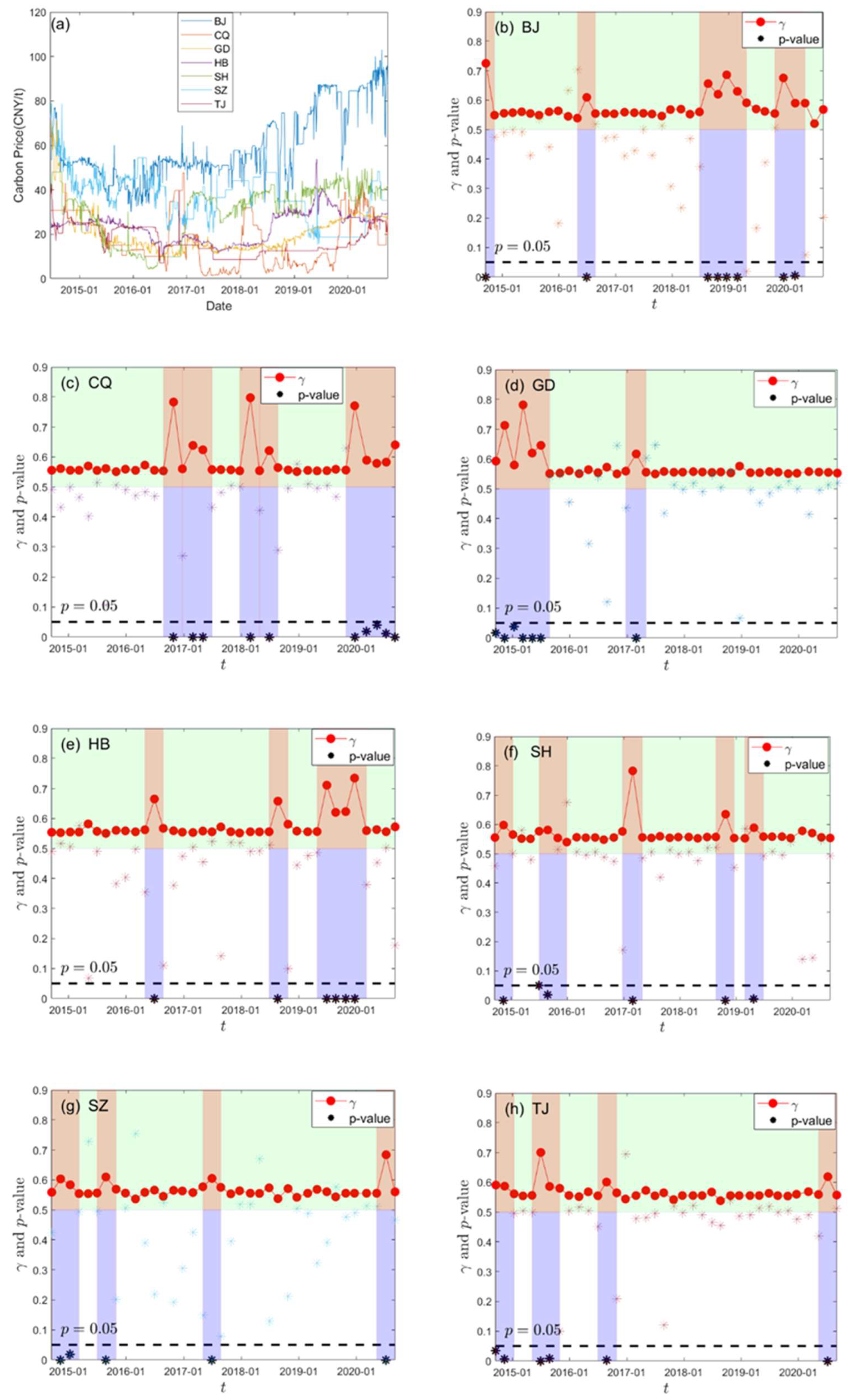
We select as sample data the carbon price data of seven pilot carbon markets in China (BJ, CQ, GD, HB, SH, SZ, and TJ) from 19 June 2014 to 30 September 2020. For comparative analysis, we select the time points where all seven markets have price data in the sample data period and delete the time points with missing data, so that each carbon market has 1525 sample data points, as shown in Figure 5a. We set the sliding window length and sliding step for each carbon market, thus obtaining time windows. We transform one-dimensional carbon price data to high-dimensional data of dimension . The evolution images and probability density distribution images of high-dimensional carbon price data of seven carbon markets are shown in the Figure A1, Figure A2, Figure A3, Figure A4, Figure A5, Figure A6 and Figure A7. On the basis of the obtained high-dimensional data, we set and , to obtain time windows. We construct the PDRN in each time window and calculate the break index of seven carbon markets and the corresponding probability using Equations (13) and (14), respectively, as shown in Figure 5b–h.
Figure 5a shows that the carbon price in each pilot area varies greatly, and the fluctuation degree is different. From Figure 5b, it is clear that the break index of the Beijing pilot market has four significant changes in four time periods. One breakpoint is detected in September 2014, with a break index of 0.7248 and a -value of 0.0000. In June 2016, one breakpoint is detected with a break index and . Four breakpoints are detected from August 2018 to February 2019, with respective break index values of 0.6559, 0.6199, 0.6859, and 0.6297, with -values of 0.0000. Two breakpoints are detected from December 2019 to March 2020, with respective break indices of 0.6753 and 0.5898, and respective -values of 0.0000 and 0.0040. From Figure 5c, we can see that the break index of the Chongqing carbon market has abrupt changes in three time periods, with 10 breakpoints detected, from October 2016 to May 2017, from February 2018 to December 2019, and from March to September 2020. The respective break indices are 0.7831, 0.6386, 0.6239, 0.7975, 0.6210, 0.7707, 0.5891, 0.5786, 0.5827, and 0.6402; the -values of the first six breakpoints and the last breakpoint are 0.0000, and those of the other breakpoints are 0.0100, 0.0290, and 0.0070, respectively. From Figure 5d, we can see that the break index of the Guangdong carbon market has two significant changes. Six breakpoints are detected from September 2014 to July 2015, with respective break index values of 0.5929, 0.7130, 0.5796, 0.7816, 0.6198, and 0.6459, and respective -values of 0.0100, 0.0000, 0.0200, 0.0000, 0.0000, and 0.0000. The second abrupt transition occurs in February 2017, with and . As can be seen from Figure 5e–h, there are relatively few breakpoints in the pilot markets of Hubei, Shanghai, Shenzhen, and Tianjin, with six detected in Hubei, occurring in June 2016, August 2018, and from June to December 2019, with respective break index values of 0.6653, 0.6582, and 0.7112, and -values of 0.0000. There are six breakpoints in the sample trading period in Shanghai and Tianjin and five in Shenzhen. Table 2 shows the time periods and index values.
As can be seen from Table 2, most breakpoints are distributed around June, which is around the declaration date of carbon trading. Important emission units in each pilot area must complete the carbon allowance payment on time, and the allowance demand of emission control enterprises has increased greatly, resulting in large fluctuations in the carbon price. Unexpected factors, such as macroeconomic factors, policies, and climate, will also have a certain impact on the carbon price. For example, Guangdong, Shanghai, Tianjin, and Shenzhen all experienced abrupt changes at the end of 2014, which were mainly caused by the issuance of the Interim Measures for the Administration of Carbon Emission Trading by the National Development and Reform Commission and the formulation of the carbon monitoring plan for the next year. The two abrupt changes in January and March of 2015 in Guangdong Province were mainly due to the issuance of the Guangdong Province 2015 Carbon Emission Quota Allocation Implementation Plan by the Guangdong Provincial Development and Reform Commission. Several breakpoints in Chongqing in 2020 were caused by the COVID-19 outbreak in early 2020. Several abrupt changes in Beijing in 2018 were possibly due to the shift of responsibility for dealing with climate change and developing the carbon market from the National Development and Reform Commission to the Ministry of Ecology and Environment. The abrupt transition in Hubei in August 2018 was mainly due to the State Council’s Opinions on Comprehensively Strengthening Ecological Environment Protection and Resolutely Fighting the Battle of Pollution Prevention and Control, issued on 18 June 2018. The breakpoint of Shanghai in November 2014 was mainly due to the Notice on Reporting Investors of Shanghai Carbon Emissions Trading Institutions issued by the Shanghai Environment and Energy Exchange in September 2014, and changes in July and August 2015 were due to the Notice on Amending the Rules of Carbon Emissions Trading issued by the Shanghai Environment and Energy Exchange in June 2015, and the carbon market entered the compliance date. The breakpoint in October 2018 was caused by the trade war between the United States and China. The breakpoint of Tianjin in July 2020 was due to the implementation of the Interim Measures for the Administration of Carbon Emission Trading in Tianjin on 1 July.
Furthermore, comparing our mutation identification results with those of Yang et al. [24] and the Bai–Perron test method [5], we can find the advantages of this method. For example, in the research of Hubei’s carbon market, the three methods found the two mutation points in June 2016 and July 2018. For the test of the pilot market in Shanghai, we found two mutation points in December 2014 and July 2015; Yang et al. also detected this mutation point on 19 December 2016, but by consulting the data, it can be found that the price of Shanghai carbon market was stable between CNY 21 and CNY 22 around 19 December 2016, so this point is a pseudo mutation point. In addition, the carbon price in the Shanghai pilot market fluctuated sharply between CNY 29.4 and CNY 35.57 in October 2018, and it fluctuated between CNY 33.05 and CNY 40.88 in April 2019. These two mutation points were detected by our method but not by Yang et al. This is also evident, in that our method fully considers the uncertainty of carbon price data and has higher accuracy and robustness than the traditional mutation detection method.
Comparing the breakpoint test results of the China and EU carbon markets, we can find that the China market has fewer breakpoints, and the EU carbon price is easily affected by external economic, financial, and political events, while the breakpoints of the China pilot markets are mainly affected by the compliance date. This also shows that the carbon price in China’s pilot market cannot well reflect the supply and demand situation, and there are problems, such as less trading volume, fewer participants, and imperfect policies.
6. Conclusions
Taking the daily closing price, the highest–lowest price series of the EU carbon market from 2 January 2013 to 30 September 2020, and the carbon price data of China pilot markets from 19 June 2014 to 30 September 2020 as the research objects, we constructed a PDRN and proposed the break index and -value to detect breakpoints in the carbon price series. We drew several conclusions: (1) based on the daily closing price data of the EU carbon market, we detected five real abrupt transitions and 14 breakpoints, occurring in March–May 2014, March 2016, March–August 2018, June–October 2019, and May–September 2020; (2) based on the daily highest–lowest price data of the EU carbon market, we detected 11 breakpoints in March 2013, March 2014, March 2016, June 2018, April–August 2019, and April–May 2020; (3) based on the data of China’s carbon market, we found eight breakpoints in the Beijing pilot market; ten in the Chongqing pilot market; seven in the Guangdong pilot market; six in the Hubei, Shanghai, and Tianjin markets; and five breakpoints in the pilot market of Shenzhen, all passing a significance test and all real. We found that the occurrence of these breakpoints was related to certain political, economic, and historical events. This discovery can prompt the government to propose carbon reform policies to guide the price trend of the carbon market to which relevant enterprises will respond, which will lead to corresponding changes in the effectiveness of the carbon market.
Compared with the traditional method based on a recurrence network, the proposed index takes into account the uncertainty of time series and is superior against noise interference and in the accurate identification of system breakpoints. The results of this study indicate that the carbon price signals of the seven pilot carbon markets in China cannot fully reflect market information. The national carbon emission trading market launched in July 2021. Whether the national carbon market can become a core policy tool to achieve carbon peak and carbon neutrality depends on its system design and also on its compatibility with other market-oriented reforms and energy conservation and emission reduction policies. The smooth operation of the carbon market should be considered as a whole, well connected with key policy nodes, and should effectively identify the abrupt structural change of the carbon price and prevent risks of policy and market failures. The method proposed in this paper to identify abrupt carbon market change points can enable the real-time analysis of carbon price information and provide theoretical support for the formulation of carbon market policy.
Author Contributions
Conceptualization, H.X., X.G., M.W., A.L.M.V. and L.T.; Data curation, M.Z.; Formal analysis, M.Z.; Funding acquisition, H.X., M.W. and L.T.; Methodology, M.Z., X.G., M.W., A.L.M.V. and L.T.; Software, M.Z., H.X., X.G. and M.W.; Supervision, M.W. and L.T.; Visualization, A.L.M.V.; Writing—original draft, M.Z.; Writing—review and editing, H.X. and M.W. All authors have read and agreed to the published version of the manuscript.
Funding
This work was supported by the National Key Research and Development Program of China (Grant No. 2020YFA0608602), the National Natural Science Foundation of China (Grant No. 72174091), Qing Lan Project of Jiangsu Province (2021), Six talent peaks project in Jiangsu Province (JY-055), and the China Postdoctoral Foundation (Grant No. 2021M691312).
Institutional Review Board Statement
Not applicable.
Informed Consent Statement
Not applicable.
Data Availability Statement
Not applicable.
Conflicts of Interest
The authors declare no conflict of interest.
Appendix A
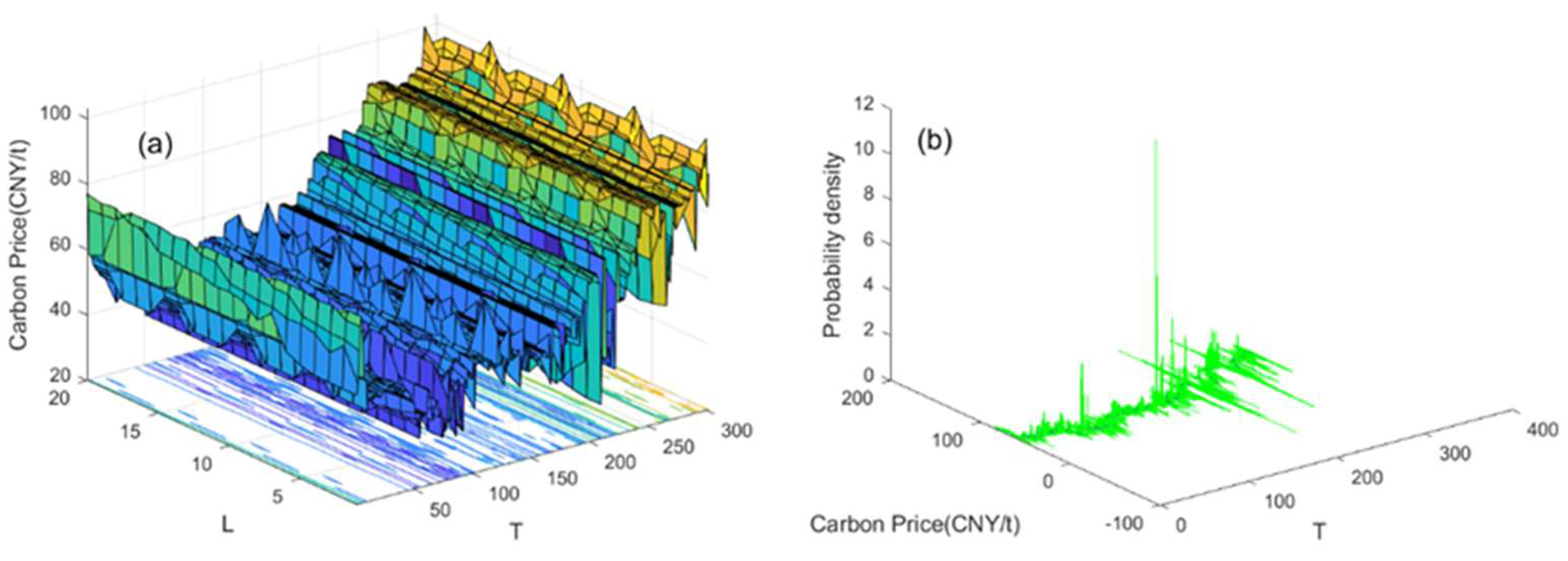
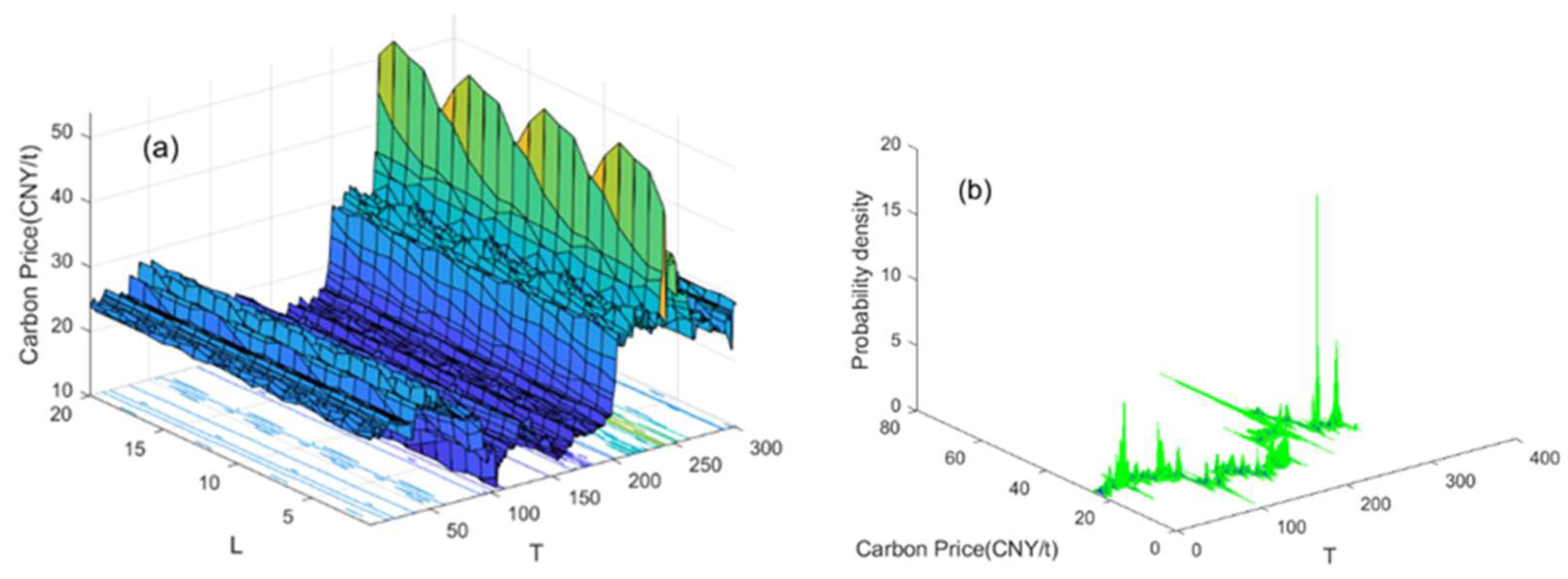
Figure A1.
Price data and probability density distribution of carbon market in Beijing, (a) evolution of daily closing price data; (b) distribution of probability density.
Figure A1.
Price data and probability density distribution of carbon market in Beijing, (a) evolution of daily closing price data; (b) distribution of probability density.

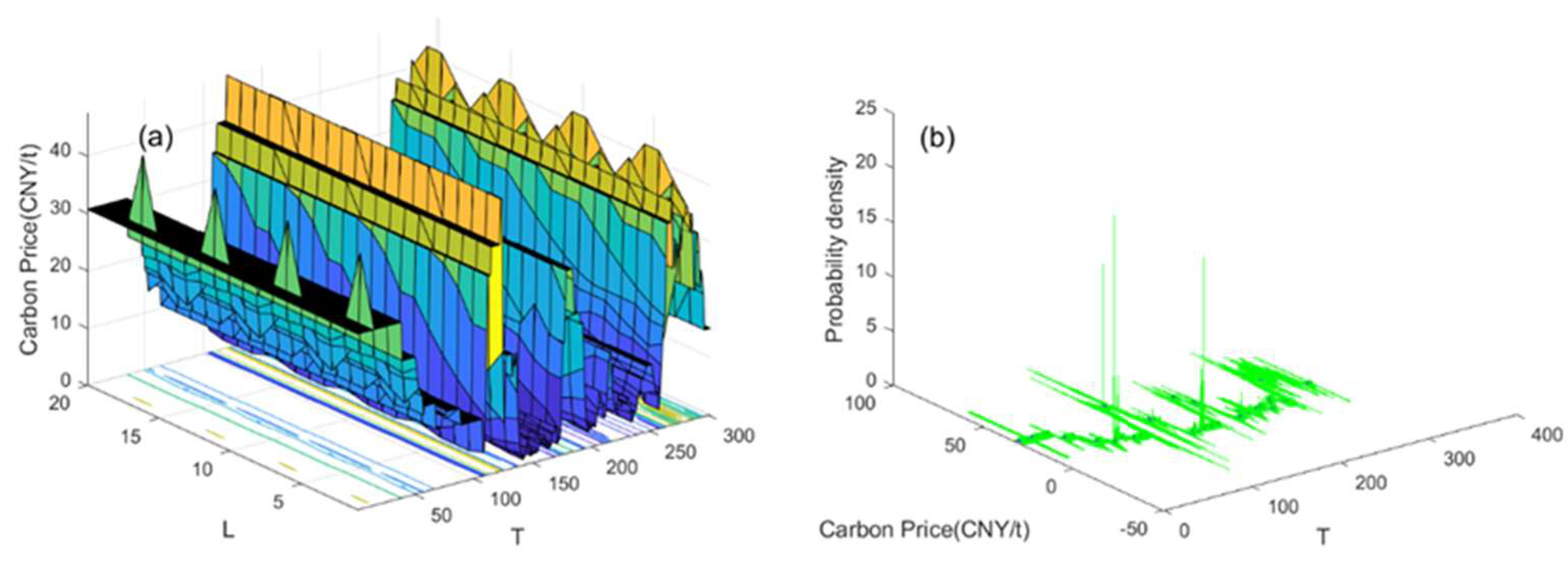
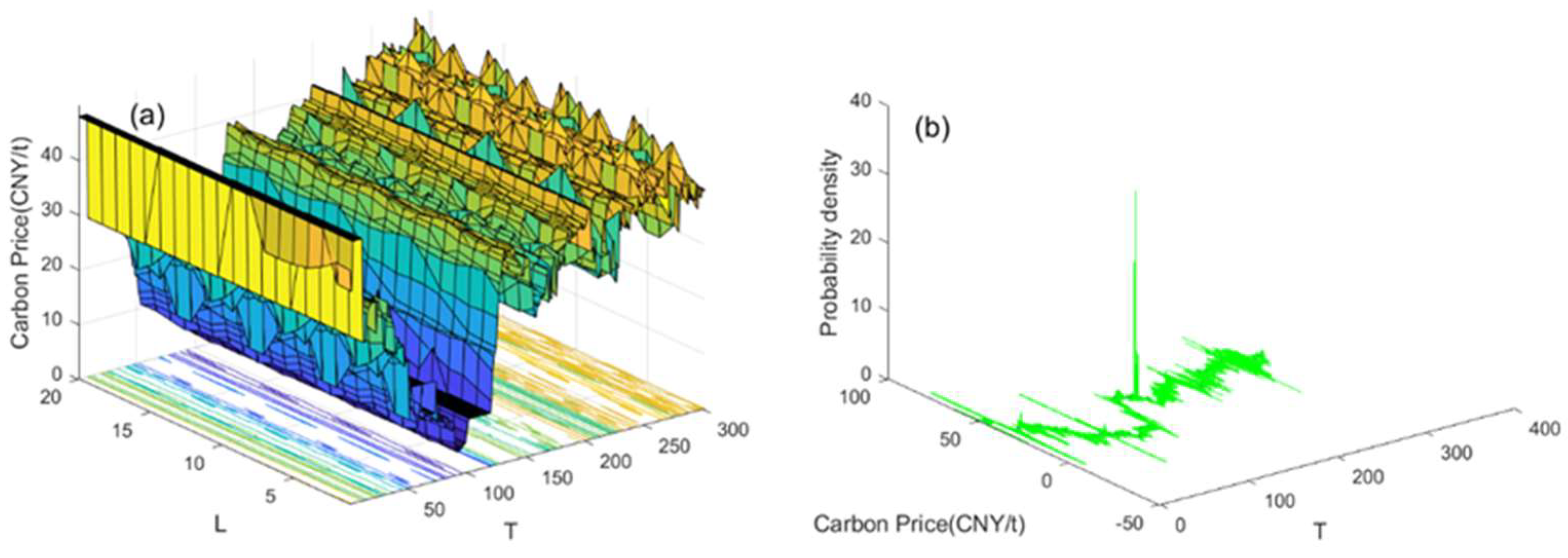
Figure A2.
Price data and probability density distribution of carbon market in Chongqing, (a) evolution of daily closing price data; (b) distribution of probability density.
Figure A2.
Price data and probability density distribution of carbon market in Chongqing, (a) evolution of daily closing price data; (b) distribution of probability density.

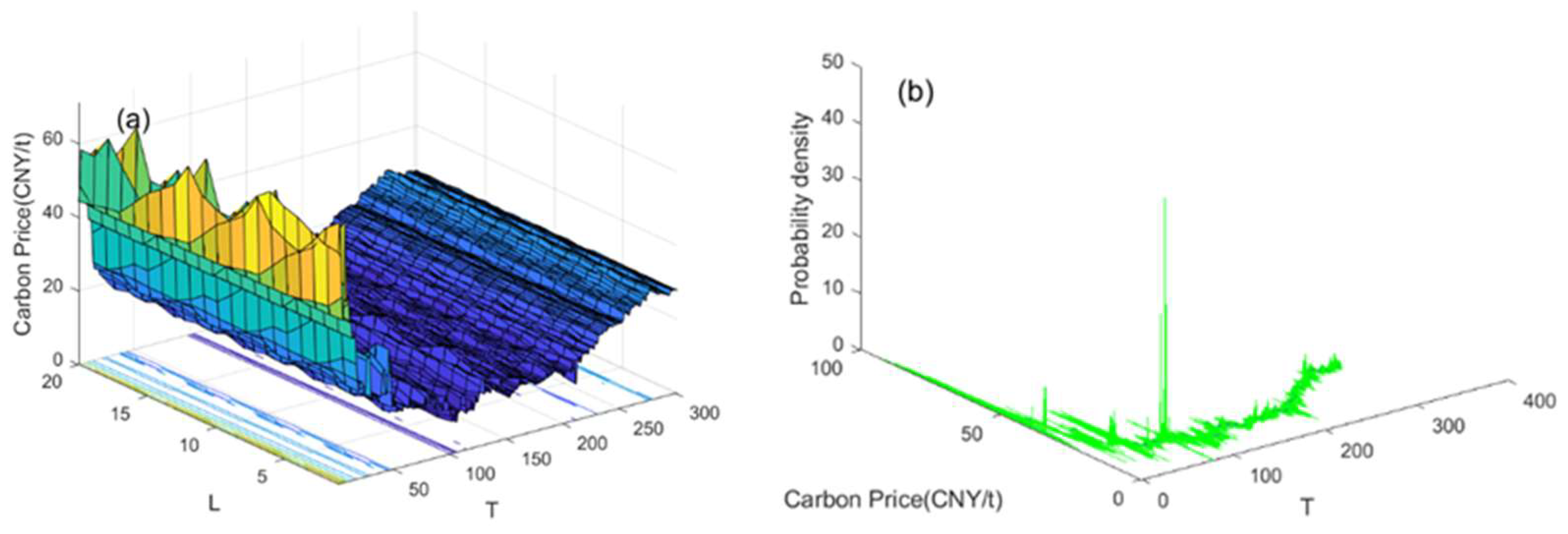
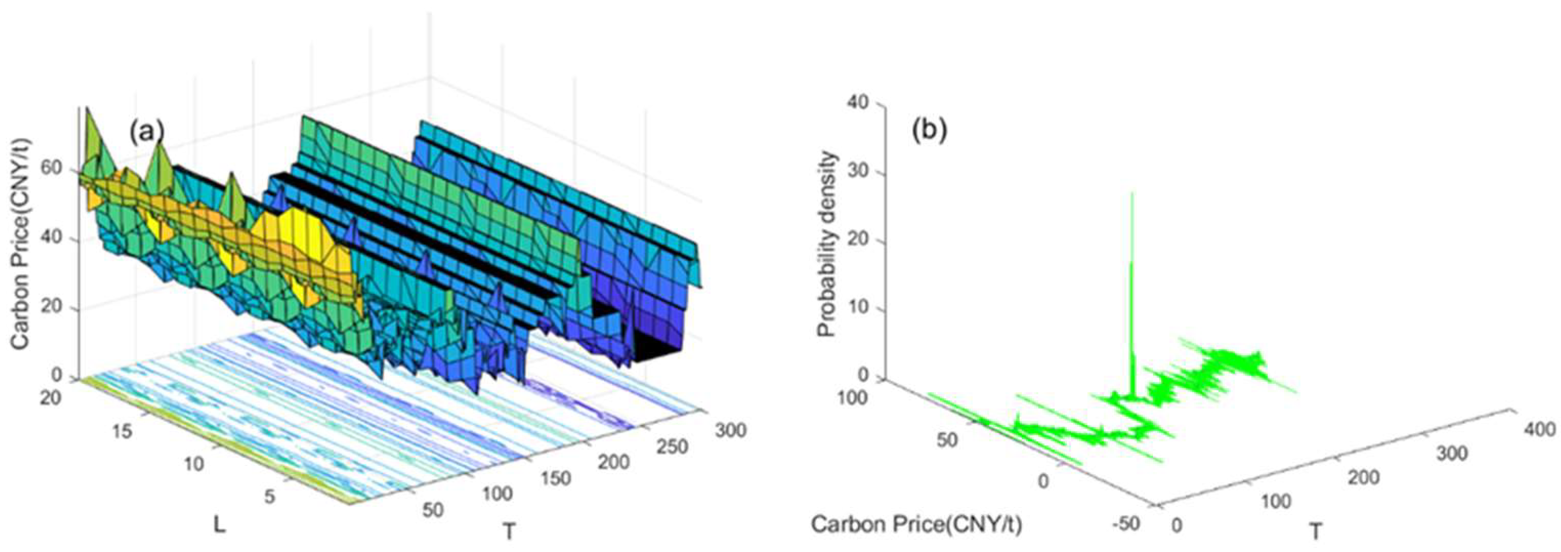
Figure A3.
Price data and probability density distribution of carbon market in Guangdong, (a) evolution of daily closing price data; (b) distribution of probability density.
Figure A3.
Price data and probability density distribution of carbon market in Guangdong, (a) evolution of daily closing price data; (b) distribution of probability density.

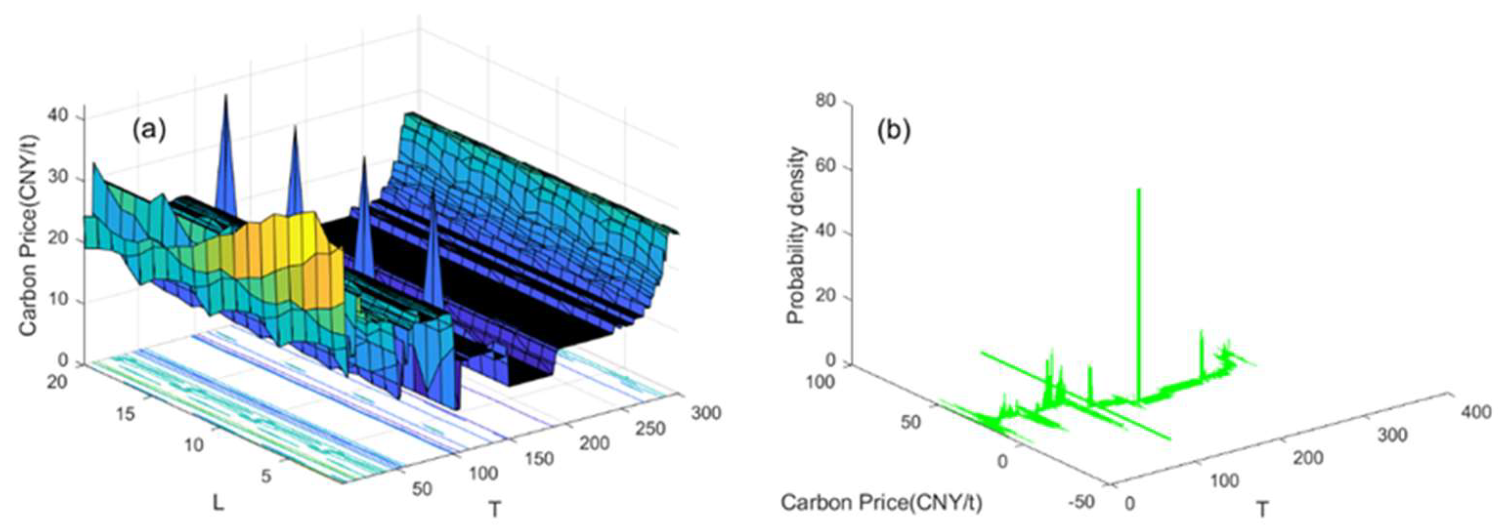
Figure A4.
Price data and probability density distribution of carbon market in Hubei, (a) evolution of daily closing price data; (b) distribution of probability density.
Figure A4.
Price data and probability density distribution of carbon market in Hubei, (a) evolution of daily closing price data; (b) distribution of probability density.

Figure A5.
Price data and probability density distribution of carbon market in Shanghai, (a) evolution of daily closing price data; (b) distribution of probability density.
Figure A5.
Price data and probability density distribution of carbon market in Shanghai, (a) evolution of daily closing price data; (b) distribution of probability density.

Figure A6.
Price data and probability density distribution of carbon market in Shenzhen, (a) evolution of daily closing price data; (b) distribution of probability density.
Figure A6.
Price data and probability density distribution of carbon market in Shenzhen, (a) evolution of daily closing price data; (b) distribution of probability density.

Figure A7.
Price data and probability density distribution of carbon market in Tianjin, (a) evolution of daily closing price data; (b) distribution of probability density.
Figure A7.
Price data and probability density distribution of carbon market in Tianjin, (a) evolution of daily closing price data; (b) distribution of probability density.

References
- Ai, M.; Wang, H.; Wen, W.; Pan, X. Analysis on the Influencing Factors of European Union Carbon Future Prices. J. Environ. Econ. 2018, 3, 19–31. [Google Scholar] [CrossRef]
- Li, Y.; Zheng, P.J. On Returns Volatility Characteristics of China’s Carbon Emissions Permits Trading Market. Sci. Technol. Manag. Land Resour. 2020, 37, 74–81. [Google Scholar]
- Hintermann, B. Allowance price drivers in the first phase of the EU ETS. J. Environ. Econ. Manag. 2010, 59, 43–56. [Google Scholar] [CrossRef] [Green Version]
- Lutz, B.J.; Pigorsch, U.; Rotfuß, W. Nonlinearity in cap-and-trade systems: The EUA price and its fundamentals. Energy Econ. 2013, 40, 222–232. [Google Scholar] [CrossRef] [Green Version]
- Perron, P. The Great Crash, the Oil Price Shock, and the Unit Root Hypothesis. Econometrica 1989, 57, 1361–1401. [Google Scholar] [CrossRef]
- Zivot, E. Further Evidence on the Great Crash, the Oil-Price Shock, and the Unit-Root Hypothesis. J. Bus. Econ. Stat. 1992, 10, 3. [Google Scholar]
- Lumsdaine, R.L.; Papell, D.H. Multiple Trend Breaks and the Unit-Root Hypothesis. Rev. Econ. Stat. 1997, 79, 212–218. [Google Scholar] [CrossRef]
- Lee, J.; Strazicich, M.C. Minimum LM Unit Root Test with One Structural Break. Econ. Bull. 2013, 33, 2483–2492. [Google Scholar]
- Bai, J.; Perron, P. Computation and analysis of multiple structural change models. J. Appl. Econom. 2003, 18, 1–22. [Google Scholar] [CrossRef] [Green Version]
- Lin, Y.N.; Lin, A.Y. Pricing the cost of carbon dioxide emission allowance futures. Rev. Futures Mark. 2007, 16, 1–16. [Google Scholar]
- Alberola, E.; Chevallier, J.; Chèze, B. Price drivers and structural breaks in European carbon prices 2005–2007. Energy Policy 2008, 36, 787–797. [Google Scholar] [CrossRef]
- Benz, E.; Trück, S. Modeling the price dynamics of CO2 emission allowances. Energy Econ. 2009, 31, 4–15. [Google Scholar] [CrossRef]
- Daskalakis, G.; Psychoyios, D.; Markellos, R.N. Modeling CO2 emission allowance prices and derivatives: Evidence from the European trading scheme. J. Bank. Financ. 2009, 33, 1230–1241. [Google Scholar] [CrossRef]
- Chevallier, J. Detecting instability in the volatility of carbon prices. Energy Econ. 2011, 33, 99–110. [Google Scholar] [CrossRef] [Green Version]
- Andrews, D.W.K. Tests for Parameter Instability and Structural Change with Unknown Change Point. Econometrica 1993, 61, 821–856. [Google Scholar] [CrossRef] [Green Version]
- Andrews, D.W.K.; Ploberger, W. Optimal Tests when a Nuisance Parameter is Present Only Under the Alternative. Econometrica 1994, 62, 1383–1414. [Google Scholar] [CrossRef]
- Ploberger, W.; Krämer, W. The Cusum Test with Ols Residuals. Econometrica 1992, 60, 271–285. [Google Scholar] [CrossRef]
- Chu, C.-S.J.; Stinchcombe, M.; White, H. Monitoring Structural Change. Econometrica 1996, 64, 1045–1065. [Google Scholar] [CrossRef] [Green Version]
- Leisch, F.; Hornik, K.; Kuan, C.M. Monitoring Structural Changes with the Generalized Fluctuation Test. Econom. Theory 2000, 16, 835–854. [Google Scholar] [CrossRef] [Green Version]
- Conrad, C.; Rittler, D.; Rotfuß, W. Modeling and explaining the dynamics of European Union Allowance prices at high-frequency. Energy Econ. 2012, 34, 316–326. [Google Scholar] [CrossRef] [Green Version]
- Wu, Z.X.; Wan, F.L.; Wang, S.P.; Hu, A.M. Test of Structural Breaks on EU ETS Carbon Price Fluctuations. J. Appl. Stat. Manag. 2015, 34, 9. [Google Scholar]
- Zhu, B.; Chevallier, J.; Ma, S.; Wei, Y. Examining the structural changes of European carbon futures price 2005–2012. Appl. Econ. Lett. 2015, 22, 335–342. [Google Scholar] [CrossRef]
- Junjun, J.; Wu, H.; Zhu, X.; Li, J.; Fan, Y. Price Break Points and Impact Process Evaluation in the EU ETS. Emerg. Mark. Financ. Trade 2019, 56, 1691–1714. [Google Scholar]
- Yang, M.; Zhu, S.Z.; Li, W.W. Study on the Effectiveness of the European Union and China Carbon Market based on Structural Breakpoints. J. Ind. Technol. Econ. 2020, 39, 92–99. [Google Scholar]
- Li, F.F.; Qian, W.D.; Xu, Z.S. Analysis on the Influencing Factors and Structural Break-points of Carbon Price in Seven Pilot Provinces and Cities. J. Xichang Coll. Nat. Sci. Ed. 2020, 34, 27–32. [Google Scholar] [CrossRef]
- Dong, F.; Gao, Y.; Li, Y.; Zhu, J.; Hu, M.; Zhang, X. Exploring volatility of carbon price in European Union due to COVID-19 pandemic. Environ. Sci. Pollut. Res. 2021, 29, 8269–8280. [Google Scholar] [CrossRef]
- Nguyen, V.C.; Vu, D.B.; Nguyen, T.H.Y.; Pham, C.D.; Huynh, T.N. Economic growth, financial development, transportation capacity, and environmental degradation: Empirical evidence from Vietnam. J. Asian Financ. Econ. Bus. 2021, 8, 93–104. [Google Scholar]
- Zheng, Y.; Yin, H.; Zhou, M.; Liu, W.; Wen, F. Impacts of oil shocks on the EU carbon emissions allowances under different market conditions. Energy Econ. 2021, 104, 105683. [Google Scholar] [CrossRef]
- Zahoor, Z.; Khan, I.; Hou, F. Clean energy investment and financial development as determinants of environment and sustainable economic growth: Evidence from China. Environ. Sci. Pollut. Res. 2021, 29, 16006–16016. [Google Scholar] [CrossRef]
- Yang, P.; Hou, X. Research on Dynamic Characteristics of Stock Market Based on Big Data Analysis. Discret. Dyn. Nat. Soc. 2022, 2022, 8758976. [Google Scholar] [CrossRef]
- Duan, K.; Ren, X.; Shi, Y.; Mishra, T.; Yan, C. The marginal impacts of energy prices on carbon price variations: Evidence from a quantile-on-quantile approach. Energy Econ. 2021, 95, 105131. [Google Scholar] [CrossRef]
- Edenhofer, O.; Kosch, M.; Pahle, M.; Zachmann, G. A whole-economy carbon price for Europe and how to get there. Eur. Energy Clim. J. 2021, 10, 49–61. [Google Scholar] [CrossRef]
- Goswami, B.; Boers, N.; Rheinwalt, A.; Marwan, N.; Heitzig, J.; Breitenbach, S.F.; Kurths, J. Abrupt transitions in time series with uncertainties. Nat. Commun. 2018, 9, 48. [Google Scholar] [CrossRef] [PubMed]
- Marwan, N.; Carmenromano, M.; Thiel, M.; Kurths, J. Recurrence plots for the analysis of complex systems. Phys. Rep. 2007, 438, 237–329. [Google Scholar] [CrossRef]
- Wang, M.; Hua, C.; Zhu, M.; Xie, S.; Xu, H.; Vilela, A.L.; Tian, L. Interrelation measurement based on the multi-layer limited penetrable horizontal visibility graph. Chaos Solitons Fractals 2022, 162, 112422. [Google Scholar] [CrossRef]
- Wang, M.; Zhu, M.; Tian, L. A novel framework for carbon price forecasting with uncertainties. Energy Econ. 2022, 112, 106162. [Google Scholar] [CrossRef]
- Parab, N.; Reddy, Y.V. The dynamics of macroeconomic variables in Indian stock market: A Bai–Perron approach. Macroecon. Financ. Emerg. Mark. Econ. 2020, 13, 89–113. [Google Scholar] [CrossRef]
- Williamson, R.C.; Downs, T. Probabilistic arithmetic. I. Numerical methods for calculating convolutions and dependency bounds. Int. J. Approx. Reason. 1990, 4, 89–158. [Google Scholar] [CrossRef] [Green Version]
- Rapp, P.E.; Darmon, D.M.; Cellucci, C.J. Hierarchical Transition Chronometries in the Human Central Nervous System. IEICE Proceeding Ser. 2014, 2, 286–289. [Google Scholar] [CrossRef]
Figure 1.
Algorithm flowchart.

Figure 2.
Identification results of breakpoints in simulation data: (a) simulation data; (b) kernel density estimation results; (c) identification results based on PDRN; (d) identification results based on traditional recurrence network.
Figure 2.
Identification results of breakpoints in simulation data: (a) simulation data; (b) kernel density estimation results; (c) identification results based on PDRN; (d) identification results based on traditional recurrence network.

Figure 3.
Identification results of breakpoints in the EU ETS based on daily highest and lowest prices: (a) probability density distribution; (b) identification results of breakpoints.
Figure 3.
Identification results of breakpoints in the EU ETS based on daily highest and lowest prices: (a) probability density distribution; (b) identification results of breakpoints.

Figure 4.
Identification result of breakpoint of daily closing price data of the EU ETS: (a) evolution of daily closing price data; (b) distribution of probability density; (c) evolution of adjacency matrix of PDRN; (d) identification of breakpoint.
Figure 4.
Identification result of breakpoint of daily closing price data of the EU ETS: (a) evolution of daily closing price data; (b) distribution of probability density; (c) evolution of adjacency matrix of PDRN; (d) identification of breakpoint.

Figure 5.
Identification results of breakpoints of carbon price data in China’s carbon market: (a) evolution of sample data in seven pilot markets; (b–h) identification results based on PDRN of seven pilot markets.
Figure 5.
Identification results of breakpoints of carbon price data in China’s carbon market: (a) evolution of sample data in seven pilot markets; (b–h) identification results based on PDRN of seven pilot markets.


Table 1.
Statistical description of sample data.
| Index | Closing Price | Highest Price | Lowest Price |
|---|---|---|---|
| Mean | 11.63625 | 11.73901 | 11.44756 |
| Max | 30.77000 | 30.1000 | 30.24000 |
| Min | 2.700000 | 2.900000 | 2.490000 |
| Std | 8.438122 | 8.532572 | 8.295047 |
| Skewness | 0.895698 | 0.910802 | 0.904718 |
| Kurtosis | 2.110458 | 2.140502 | 2.133726 |
| JB test | 333.3657 *** | 338.0814 *** | 335.3738 *** |
| ADF test | −1.792782 (−3.433422) | −1.830002 (−3.433424) | −1.836951 (−3.433424) |
Note: *** denotes significance at 1% level.
Table 2.
Breakpoint test results of carbon price in several pilot markets in China.
| Pilot Area | Break Time | Break Index γ | p-Values |
|---|---|---|---|
| Shanghai | 12 November 2014 | 0.5981 | 0.0040 |
| 1 July 2015 | 0.5772 | 0.0490 | |
| 26 August 2015 | 0.5814 | 0.0180 | |
| 28 February 2017 | 0.7834 | 0.0000 | |
| 24 October 2018 | 0.6351 | 0.0000 | |
| 26 April 2019 | 0.5889 | 0.0040 | |
| Shenzhen | 12 November 2014 | 0.6033 | 0.0000 |
| 12 January 2015 | 0.5836 | 0.0160 | |
| 26 August 2015 | 0.6098 | 0.0000 | |
| 29 June 2017 | 0.6052 | 0.0000 | |
| 7 July 2020 | 0.6838 | 0.0000 | |
| Tianjin | 17 September 2014 | 0.5907 | 0.0300 |
| 12 November 2014 | 0.5870 | 0.0080 | |
| 1 July 2015 | 0.7004 | 0.0000 | |
| 26 August 2015 | 0.5860 | 0.0060 | |
| 24 August 2016 | 0.6009 | 0.0010 | |
| 7 July 2020 | 0.6190 | 0.0000 |
Publisher’s Note: MDPI stays neutral with regard to jurisdictional claims in published maps and institutional affiliations. |
© 2022 by the authors. Licensee MDPI, Basel, Switzerland. This article is an open access article distributed under the terms and conditions of the Creative Commons Attribution (CC BY) license (https://creativecommons.org/licenses/by/4.0/).
Share and Cite
MDPI and ACS Style
Zhu, M.; Xu, H.; Gao, X.; Wang, M.; Vilela, A.L.M.; Tian, L. Identification of Breakpoints in Carbon Market Based on Probability Density Recurrence Network. Energies 2022, 15, 5540. https://doi.org/10.3390/en15155540
AMA Style
Zhu M, Xu H, Gao X, Wang M, Vilela ALM, Tian L. Identification of Breakpoints in Carbon Market Based on Probability Density Recurrence Network. Energies. 2022; 15(15):5540. https://doi.org/10.3390/en15155540
Chicago/Turabian StyleZhu, Mengrui, Hua Xu, Xingyu Gao, Minggang Wang, André L. M. Vilela, and Lixin Tian. 2022. "Identification of Breakpoints in Carbon Market Based on Probability Density Recurrence Network" Energies 15, no. 15: 5540. https://doi.org/10.3390/en15155540
Note that from the first issue of 2016, this journal uses article numbers instead of page numbers. See further details here.