
Surface-Related and Internal Multiple Elimination Using Deep Learning

1
School of Earth Sciences, Northeast Petroleum University, Daqing 163318, China
2
Key Laboratory of Continental Shale Hydrocarbon Accumulation and Efficient Development, Ministry of Education, Northeast Petroleum University, Daqing 163318, China
*
Author to whom correspondence should be addressed.
Energies 2022, 15(11), 3883; https://doi.org/10.3390/en15113883
Submission received: 12 April 2022
/
Revised: 4 May 2022
/
Accepted: 18 May 2022
/
Published: 25 May 2022
(This article belongs to the Special Issue Artificial Intelligence Techniques in Oil and Gas Exploration and Development)
Abstract
:Multiple elimination has always been a key, challenge, and hotspot in the field of hydrocarbon exploration. However, each multiple elimination method comes with one or more limitations at present. The efficiency and success of each approach strongly depend on their corresponding prior assumptions, in particular for seismic data acquired from complex geological regions. The multiple elimination approach using deep learning encodes the input seismic data to multiple levels of abstraction and decodes those levels to reconstruct the primaries without multiples. In this study, we employ a classic convolution neural network (CNN) with a U-shaped architecture which uses extremely few seismic data for end-to-end training, strongly increasing the neural network speed. Then, we apply the trained network to predict all seismic data, which solves the problem of difficult elimination of global multiples, avoids the regularization of seismic data, and reduces massive amounts of calculation in traditional methods. Several synthetic and field experiments are conducted to validate the advantages of the trained network model. The results indicate that the model has the powerful generalization ability and high calculation efficiency for removing surface-related multiples and internal multiples effectively.
1. Introduction
Multiple elimination has always been challenging in the field of seismic data processing. Based on the downward reflection interface where the energy bounces frequently occur, multiples are categorized into surface-related multiples and internal multiples. At present, multiple elimination methods usually include two categories: filtering methods and wave equation-based methods. The filtering method [1,2,3,4] works when multiples and primaries can be separated by parabolic move-out in time domain or mapped into different areas in other domains. However, move-out discrimination between primaries and multiples from complex targets and high scattering overburdens are typically small, particularly for internal multiples in field data. The filtering method may seriously damage primaries and thus cannot meet the requirements of multiple elimination. The method based on a wave equation includes the feedback method (SRME, surface-related multiple elimination), the sparse inversion method (EPSI, estimation of primary by sparse inversion), and the inverse scattering series method (ISS) for surface-related multiple elimination; the common focus point (CFP) method, the virtual event method, and the Marchenko method (MME, Marchenko multiple elimination) are for internal multiple elimination.
SRME [5] is fully data-driven and has been successfully applied in field data. However, this method requires that the seismic traces are full wavefield data using fixed-spread geometry configuration. Particularly, field data always requires regularization. In addition, due to the fact that the predicted surface-related multiples have the problem of mismatching at phase, amplitude, and travel time, it is necessary to use the adaptive matching subtraction algorithm to remove surface-related multiples in seismic data. EPSI [6,7,8] performs primaries in seismic data through iterative inversion based on the inversion theory without the steps of multiple prediction and adaptive matching subtraction in SRME. Thus, the damage generated by adaptive matching subtraction to primary is avoided. However, iterative implementation of EPSI in multiple elimination requires extensive computation; meanwhile, unstable source wavelet estimation makes the application of the method more challenging. ISS [9,10,11] can predict given-order internal multiples each time without prior information of subsurface but the amount of computation is still massive, particularly for 3D seismic data. CFP [12] extrapolates seismic records to the subsurface interface and predicts related internal multiples. This method requires velocity information to obtain an accurate focusing operator. MME [13,14,15,16] is an internal multiple elimination method developed in recent years, and the method has achieved excellent results in both synthetic and field data [17]. However, the Marchenko method requires high-density seismic data of regularly sampled and co-located sources and receivers [18]. High density indicates that the best internal multiple elimination results will be obtained only when the receiver space is small, particularly in complex geological regions. Therefore, it is difficult to be widely applied in field data because of the large acquisition and computation costs.
As new technology in the research of machine learning algorithms emerges, deep learning proposed by Hinton et al. [19] has been highly considered by both academia and industry. Its motivation is to establish and simulate the neural network like a human brain for analytical learning which has been pervasively used in speech recognition, image recognition, natural language processing, CTR prediction, big data feature extraction, etc. The deep learning method is fully data-driven and does not need to manually extract data features for model building. It can represent attribute categories or features by combining low-level features with generating more abstract high-level features to find effective features of data and have a certain generalization ability.
In the past few years, deep learning has proven noteworthy achievements in several applications, and has developed rapidly in the field of hydrocarbon exploration [20,21,22,23,24,25,26]. We call this intelligent exploration. In multiple elimination, Siahkoohi et al. [27] utilize the shot records with and without surface-related multiples, obtained via EPSI or SRME, as input-output training pairs of the convolutional neural network (CNN). The accuracy of multiple elimination by the trained neural network considerably increases. Yu et al. [28] utilize CNN architecture for random noise, linear noise, and surface-related multiple elimination in seismic data and obtain favorable results in synthetic data. By applying transfer learning, the trained neural network can successfully remove random noise and linear noise in field data. Based on the deep learning technique, Qu et al. [29] reconstruct the near offset of seismic data and then use the reconstructed data as the input for subsequent surface-related multiple elimination. The neural network trained only by synthetic data indicates satisfactory results in field data. Vrolijk and Blacquière [30] subsample all shot records with and without receiver-ghost for training the convolutional neural network, which can remove the source-ghost from the coarsely sampled common-receiver records. Song et al. [31] eliminate surface-related multiples based on a deep neural network and obtain satisfying results in synthetic data from industry.
On the basis of previous techniques, we present a multiple elimination method using deep learning with a U-net proposed by Hinton and Salakhutdinov [32]. Ronneberger [33] applied a U-net in medical image segmentation, which can be trained end-to-end from very few images with a high speed. In this study, the trained neural network model is applied to remove surface-related multiples and internal multiples, which can address the problem of difficult elimination of global multiples. We choose the synthetic data with and without surface-related multiples which are simulated using sigsbee2b model provided by Society of Exploration Geophysicists (SEG). The shot records with and without internal multiples are obtained via MME [34] using syncline model-simulated data. The field data with and without multiples are obtained via the multiple suppression method based on iterative inversion [35]. In addition, for other new data sets, we can make the training data set according to the specific seismic data characteristics and geological conditions. For example, if seismic data belong to Marine Seismic Data with well-developed surface-related multiples, we will choose SRME or Radon transform, etc., to eliminate multiples and obtain training sets; if onshore seismic data includes mainly internal multiples, we can choose the virtual events method or the multiple suppression method based on iterative inversion, etc., to eliminate multiples. Few synthetic records and field data are set as input-output training pairs of the neural networks, respectively. The trained neural network can effectively identify multiples and primaries, the former of which are subsequently removed in all seismic data. In addition, the deep learning method avoids the regularization of seismic data that most wave equation-based methods require for predicting multiples and reduces the large amount of calculation, especially for field data.
The paper is organized as follows. After introduction, we briefly review the theory of multiple elimination using deep learning. Then, we introduce the deep U-net architecture and network training, followed by several synthetic experiments together with field data, which validates the effectiveness of our approach. Finally, conclusions are drawn after detailed analyses and discussion.
2. Theory
2.1. Multiple Elimination Using Network
Assuming that the preprocessed seismic records contain only primaries and multiples, which can be expressed as:
where denotes the total wavefield includeing primaries () and multiples (M). The objective of multiple elimination is to remove from , namely:
Traditional multiple elimination methods include two steps. First, multiples are predicted using the model information. Then, due to the mismatch of phase, amplitude, and travel time during the prediction process, the adaptive matching subtraction algorithm is utilized to remove multiples in seismic data.
where represents the seismic records without multiples, indicates predicted multiples and is adaptive filter which reduces the deviation between the predicted and actual multiples. However, adaptive matching subtraction usually influences the integrity of primaries. The multiple elimination method using deep learning can distinguish primaries and multiples by combining low-level features and thus form more abstract high-level features. Moreover, the method is fully data-driven, without artificially extracting data features to the model construction process. As long as the training set is abundant enough, the trained network will indicate strong generalization ability and can be widely used in multiple elimination with few computation costs. Therefore, the deep learning method is selected to eliminate multiples in this study; the method establishes the relationship between and with the following formula:
where stands for primaries obtained by neural network model learning. Network describes the neural network architecture, equivalent to multiple filters. represents neural network parameters including the network layers , the number of kernels , the weight matrix W, and bias b, etc. is written as:
According to the above description, the objective function of the neural network can be expressed as:
where denotes the norm, and represents the number of training data pairs. Through network training, we can obtain the reconstructed primaries.
2.2. Network Architecture
Although the convolutional neural network has been used for some time, its success is limited by the size of available training sets and the network size. U-net uses only scarce data for end-to-end training with a fast neural network speed and has been successfully applied in the medical field [36], in which the limited amount of training data resembles those of our case. Furthermore, some scholars have applied U-net in hydrocarbon exploration. Vrolijk and Blacquiere [30] use U-net to remove source ghosting of coarsely sampled common-receiver data. Zhang [37] utilizes U-net to image prestack reflection seismic data. They all prove that U-net can alleviate the problem of few samples, describe the characteristics before and after multiple elimination better, improve the calculation efficiency of field data, and promote the development of industrial production. Experiments of various network characteristics also confirm that U-net network can better eliminate multiples. For example, compared with DDA (Deep Denoising Autoencoder) [38], on the same situation, the prediction accuracy of U-net is always higher. This study defines convolutional neural network model of U-net type with convolutional encoders and convolutional decoders based on TensorFlow deep learning framework [39] to eliminate surface-related multiples and internal multiples.
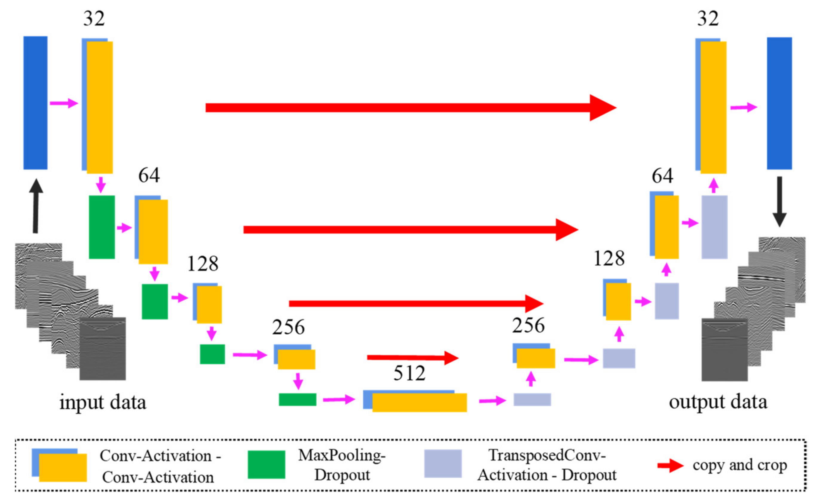
Figure 1 presents the deep U-net architecture that is composed of encoder and decoder connected by a bridge. The depth of network is 4. The encoder consists of two convolution layers: a max pooling layer (downsample), and dropout for special extraction of seismic data information. The decoder also consists of two convolution layers: one transposed convolutional layer (upsample), and a dropout, which maps the low dimensional data contained in the primary to the high-dimensional space and reconstructs the primary. Each of the convolution layers and transposed convolutional layers is followed by exponential linear units (). The bridge is similar to encoders except for the max pooling layer and dropout.
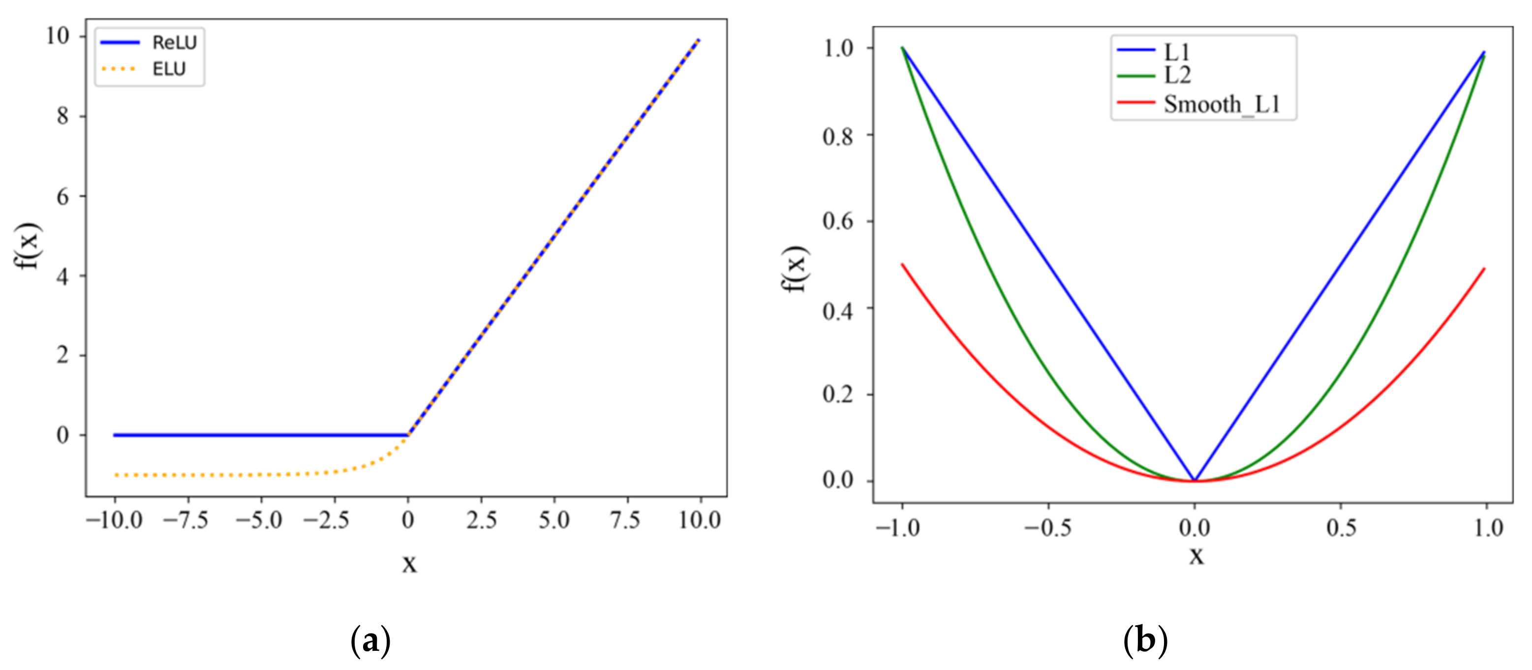
Activation function plays an essential role in artificial neural network model learning and the understanding of complex and nonlinear functions. Since rectified linear unit () activation function was proposed by Alex et al. [40], it has been widely used due to its ability to sparsely activate neurons. The exponential linear unit () activation function [41] possesses all the advantages of (Figure 2a). The negative part of can make itself more robust when the input changes or there is noise in the input data. It can also accelerate the convergence speed and remove the dead zone of . The sparse model realized by can better extract relevant features and fit our training data. Thus, we choose the for network model training to handle the seismic data properly, and it can be formulated as:
where is the real primary , and is a constant.
2.3. Network Training
In this study, neural network training adopts the supervised learning method. The training set of supervised learning requires input and output, namely, features and objectives. An optimal network model is obtained by training the existing sample, followed by the process of mapping other unknown input data into corresponding outputs for prediction. Subsequently, we prepare the training data set and choose the appropriate loss function and optimization algorithm to obtain the optimal network model.
The data with and without surface-related multiples or internal multiples are input as labeled training sets for network training. It is worth noting that to increase the convergent speed of the network model training, the input data set is required to be normalized, particularly for field data. Since the ELU activation function is selected for the neural network, the amplitude of data set is normalized to [–1, 1], and the calculation formula is as follows:
where is the data set, is the normalized value, is the global maximum absolute amplitude of the data set.
The loss function is a non-negative real value function which is used to estimate the inconsistency between labeled data and predicted data. Popular loss functions include mean square error (MSE, L2), mean absolute error (MAE, L1), and smooth L1 loss function (Figure 2b). When the regression targets are unbounded, training with L2 loss can require careful tuning of learning rates to avoid exploding gradients. Smooth L1 loss function eliminates this sensitivity [42]. In addition, it possesses all the advantages of the L1 loss function with a faster converge speed and the gradient change is relatively small. We use smooth L1 loss function to calculate Equation (6) for network training, as presented in Equation (9) below.
where is the difference between the real primary and the predicted primary .
In network training, the ADAM (Adaptive Moment Estimation) optimizer [43] is selected to update each parameter by iteration with a learning rate starting at 10−3. It is suitable for solving optimization problems with large-scale data and parameters, in addition to problems including strong noise or sparse gradients, particularly for field data. In addition, in the initialization phase, we give each network connection weight a small random number and initialize bias of each neuron with a random number [44]. The number of filters for the model are tested in Figure 3 (take Sigsbee2B model for example). It is difficult to understand from the charts which model indicates the best quality. Therefore, we calculate the standard error of the test data (Table 1). We can observe that the best quality presents a model with the following parameters: the initial number of filters is 32 and the number of U-net blocks is 5. The number of filters is increased by twice with downsampling and decreased by twice with upsampling.

Table 1.
The standard error of the test data.
| Number of Filters | Standard Error |
|---|---|
| Filters_[32, 64, 128, 256, 512] | 0.012465 |
| Filters_[8, 16, 32, 64, 128] | 0.013284 |
| Filters_[16, 16, 32, 32, 64, 64, 128, 128, 256, 256] | 0.014788 |
| Filters_[32, 64, 128] | 0.015832 |
| Filters_[16, 32, 64, 128, 256] | 0.016310 |
| Filters_[16, 32, 64] | 0.016393 |
| Filters_[32, 32, 64, 64, 128, 128, 256, 256, 521, 512] | 0.021159 |
| Filters_[8, 16, 32] | 0.026624 |
| Filters_[8, 8, 16, 16, 32, 32, 64, 64, 128, 128] | 0.031513 |
3. Experiments
In this section, we use a Sigsbee2B model with and without synthetic surface-related multiples, a synclinal model with and without synthetic internal multiples, and field data with and without multiples to validate the effectiveness of the proposed method.
3.1. Sigsbee2B Model Data Example
Firstly, the sigsbee2b model synthetic data is used to train and test the network of the elimination of surface-related multiples. The test of surface-related multiples is provided by SEG with a finite-difference scheme using the sigsbee2b velocity model from Figure 4. The velocity model size is 80,000 ft × 30,000 ft, grid size is 25 ft × 25 ft, dominant frequency is 20 Hz, and the maximum frequency is 40 Hz. Sources and receivers are distributed 25 ft below water surface. There are 500 shot records with a spacing of 150 ft and 348 traces per shot record with a lateral interval of 75 ft. The time sampling interval is 8 ms and the seismic reflection record is 12 s. The direct wave has been removed.
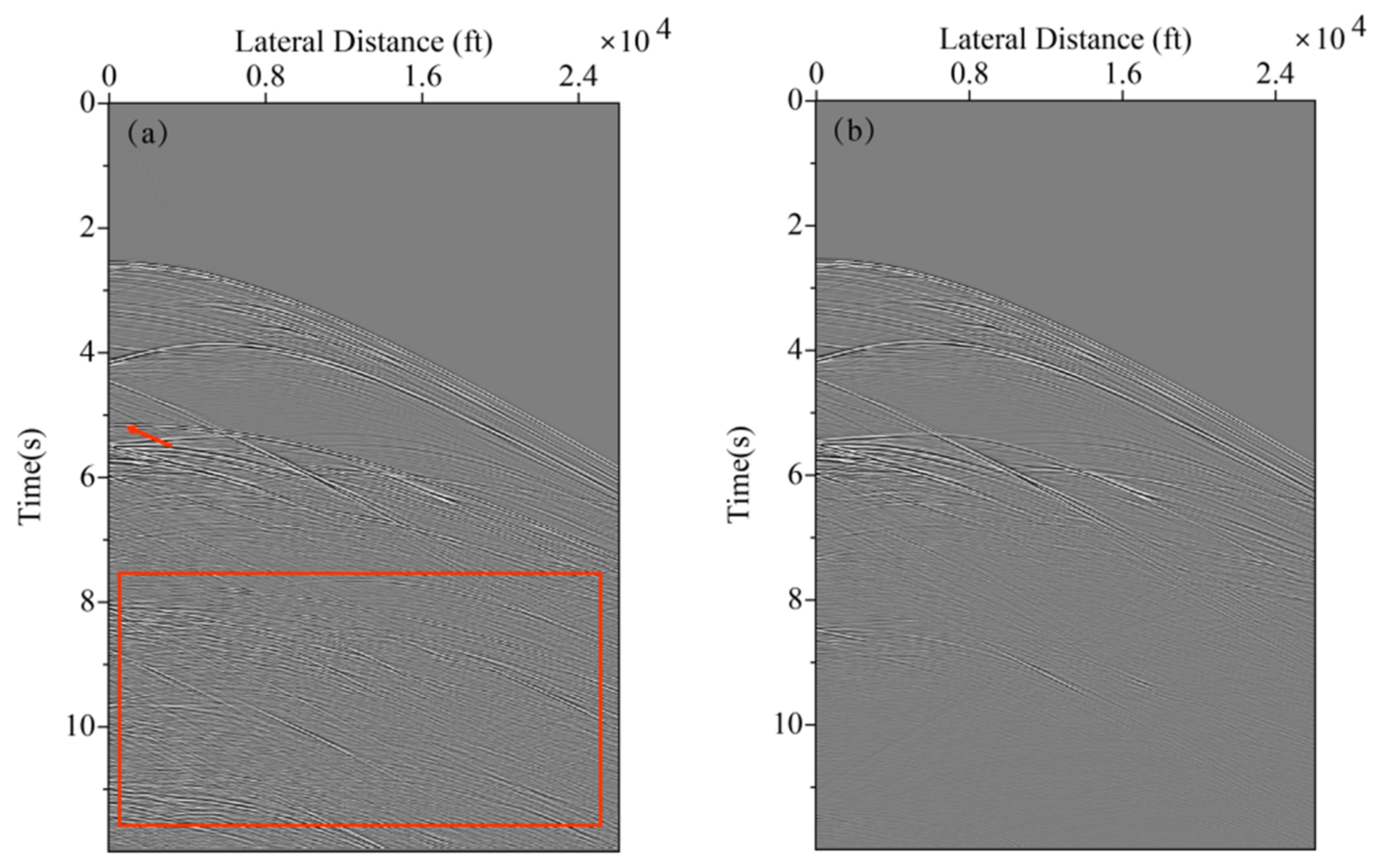
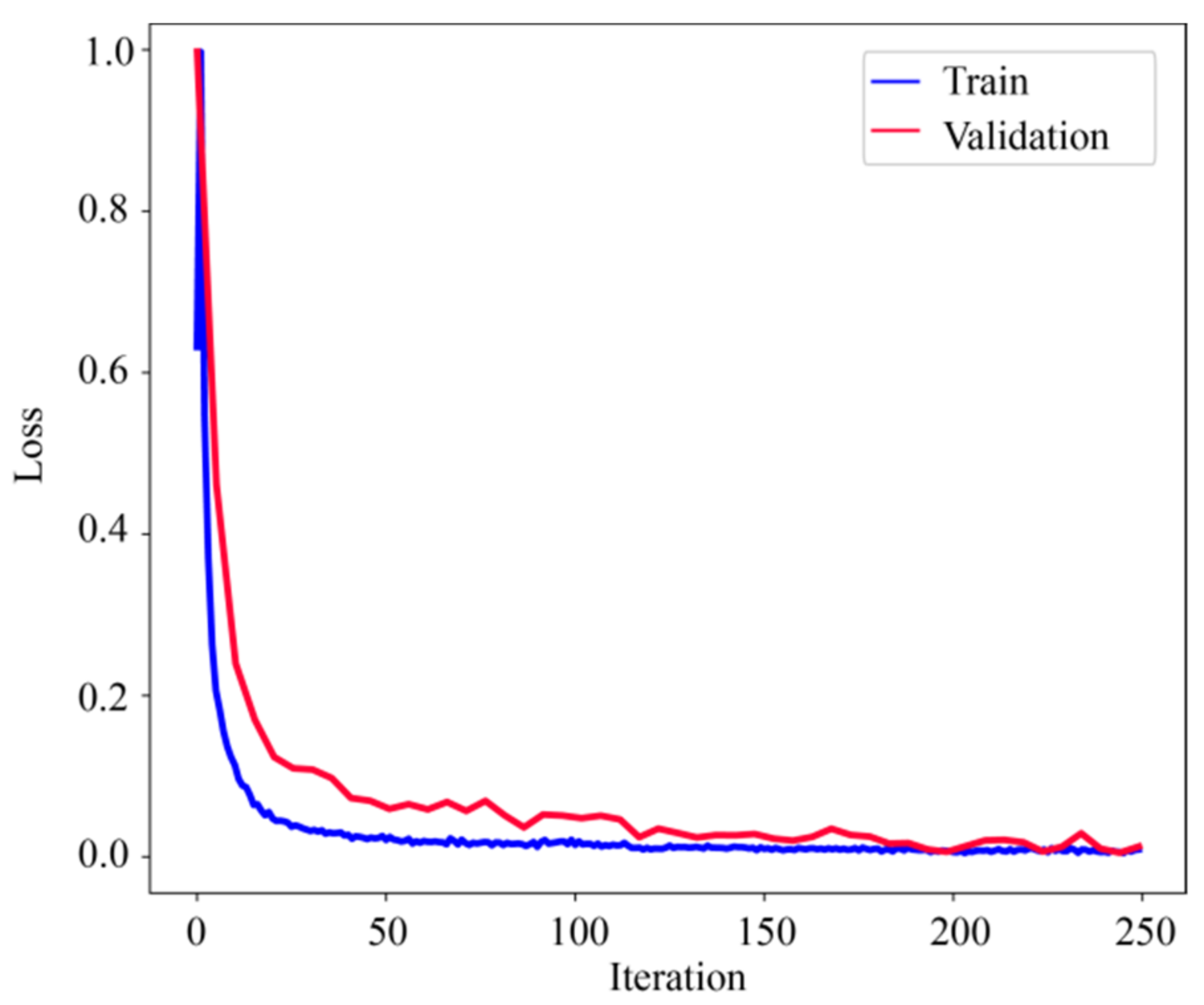
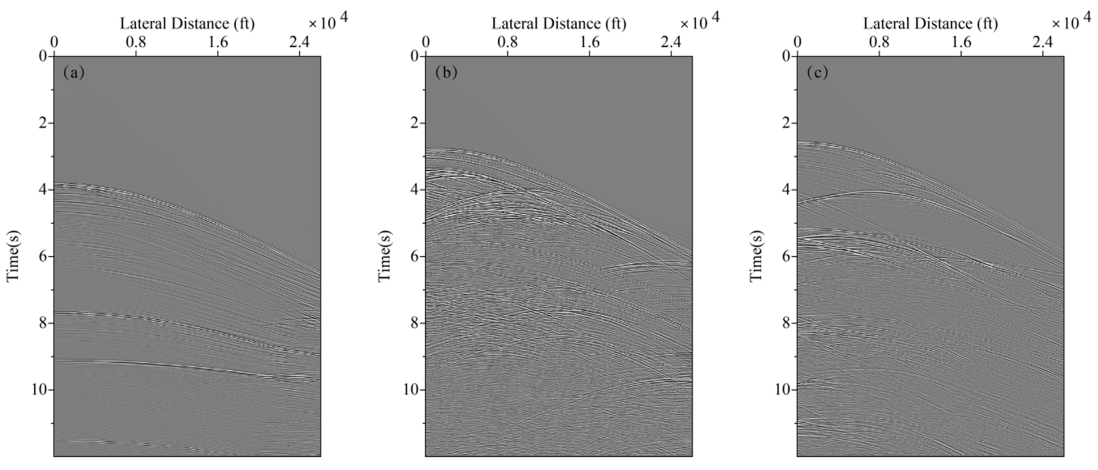
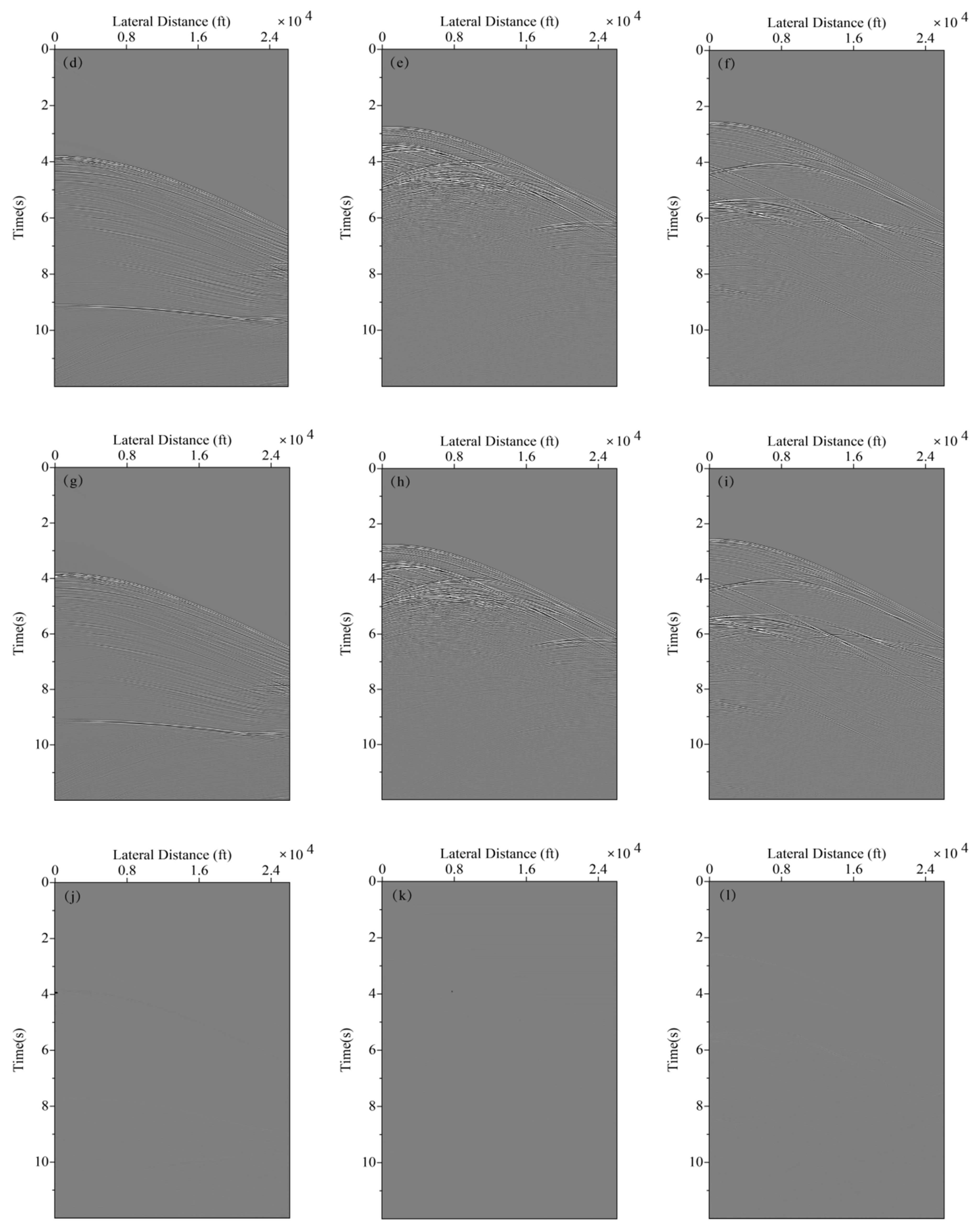
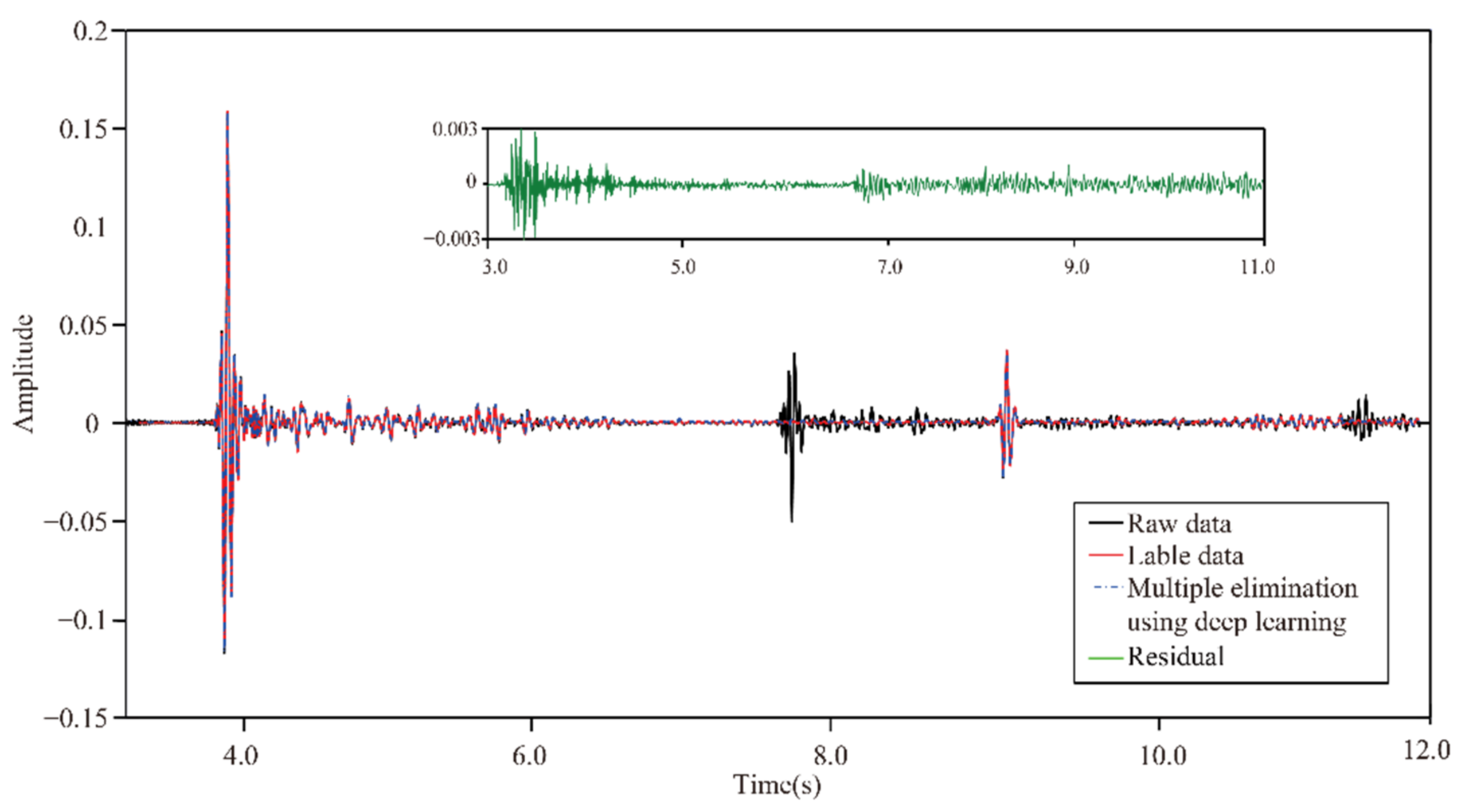
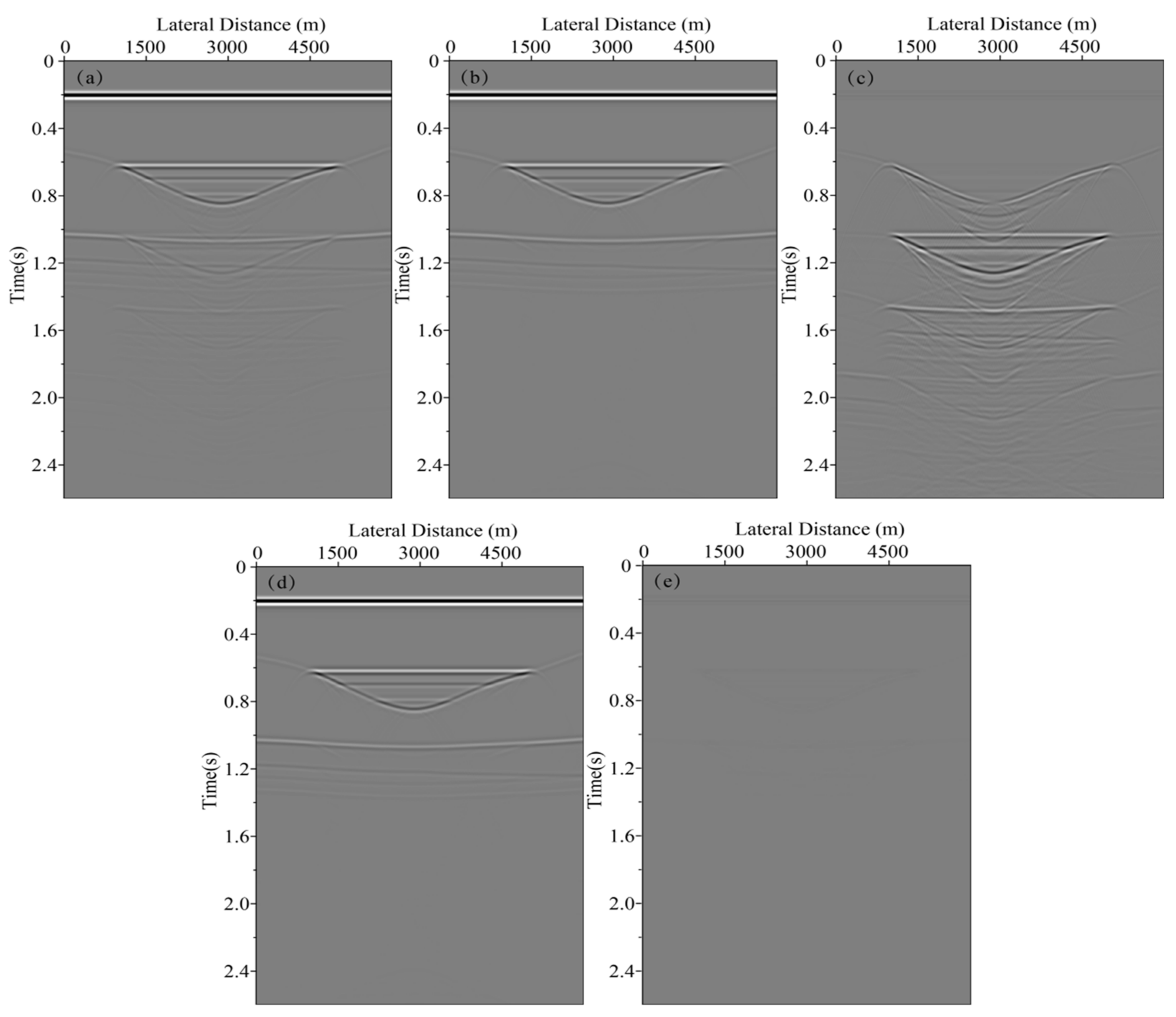
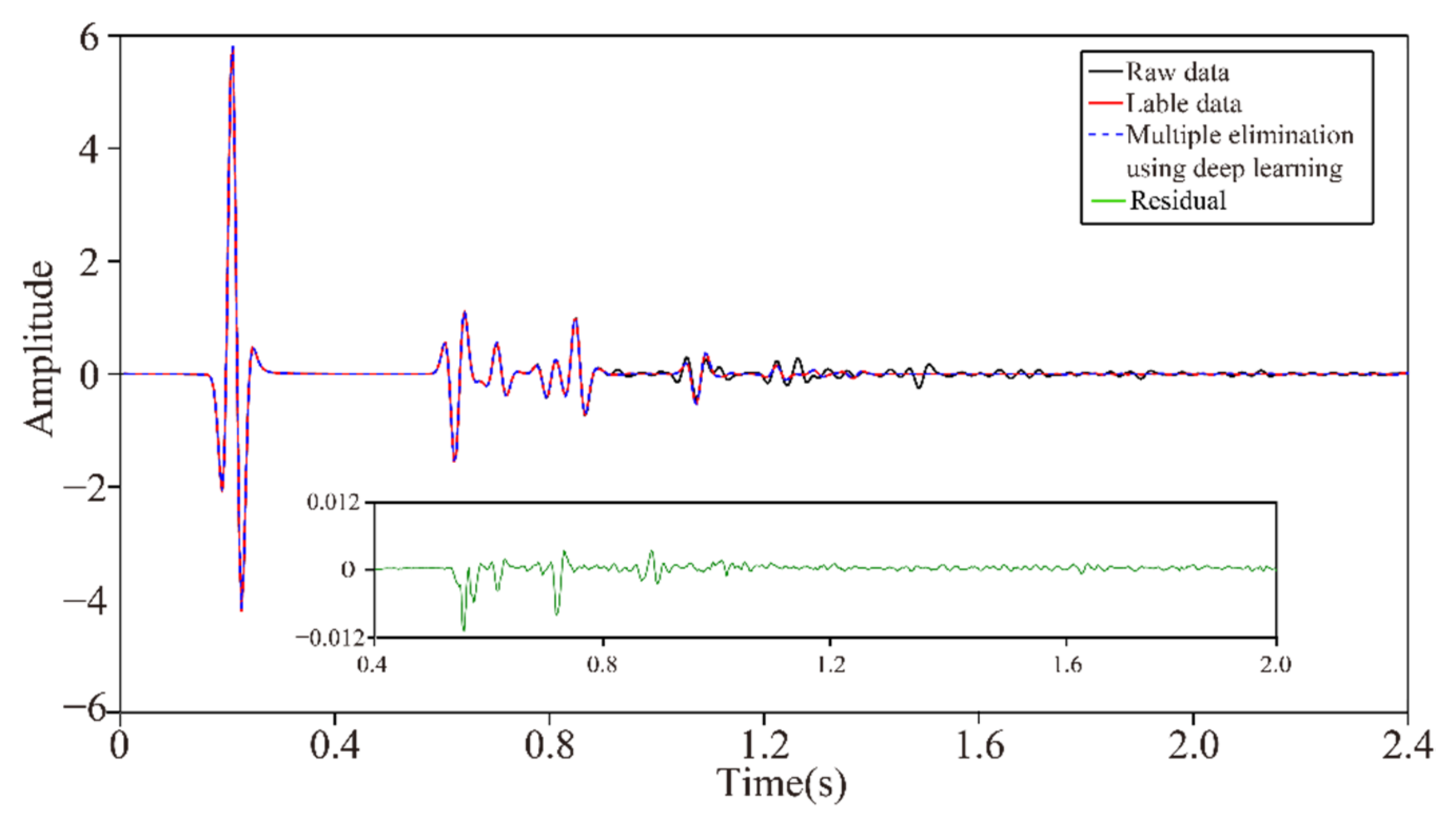
In neural network training, considering the calculation efficiency and adjacent data similarity in seismic data, 20 pairs of shot records are selected with intervals equal to the training set, and other part of shot records are used for the test set. The convolution kernel length of the network convolution layer is 5 and the stride is 2. We choose “padding same” for filling to ensure that the input dimension and output dimension of the convolution layer are consistent. The length of maximum pool is 2 and the pool_strides is 2. Batchsize is 32 for one training. Each downsampling and upsampling layer inactivates neurons with a probability of 5% (dropout_rate = 0.05) to prevent overfitting in the training process, improving the generalization ability of the deep neural network. Training time per one batch of size 32 traces is 0.25 s, all training time with batch size 32 is 3:49:45 h. When the neural network is well trained, it only takes an average of 2:14 min to calculate all shot records. Figure 5 presents one pair of shot records with and without surface-related multiples in the training set. Surface-related multiples are mainly developed in the position as indicated by the red arrow and red box. Figure 6 displays the loss function for training the network model using the training data sets. Shot records with surface-related multiple elimination using deep learning are illustrated in Figure 7. Figure 7a–c respectively present the 10th, 150th, and 310th shot records with surface-related multiples, which are distributed in different positions of the model for better reflection of the training network quality. Figure 7d–f present the 10th, 150th, and 310th shot records without surface-related multiples. Figure 7g–i present the 10th, 150th, and 310th shot records with surface-related multiple elimination using deep learning, respectively. Figure 7j–l display the difference between label data and multiple elimination results using the trained network. Zero-offset data with surface-related multiples, zero-offset data after the elimination of surface-related multiples using deep learning, and zero-offset data without surface-related multiples are displayed in Figure 8a,b,d, respectively. In Figure 8, the differences between a and b, d and b are displayed in c and e, respectively. Figure 9 presents the comparison of the 37th trace from Figure 7a,d,g. The black line is generated from the original shot record depicted in Figure 7a, the red line comes from the shot record without multiples presented in Figure 7d, the blue dashed line is obtained from the shot record with surface-related multiple elimination presented in Figure 7g, and the green line is the difference between label data and results. It can be observed from Figure 7j–l and Figure 8e that the residual between the data after surface-related multiple elimination using trained network and label data is tiny. The blue dashed line and the red line are generally consistent with each other. The average correlation of the test set exceeds 96.62% when the number of epochs is 250, suggesting a strong ability of surface-related multiple elimination.
3.2. Data Example of the Synclinal Model
Figure 10 exhibits the synclinal velocity model that includes a syncline structure with inclined interface and thin interbedding. We compute the synthetic data with a finite-difference time-domain modeling code for 601 shot records that each contain 601 traces. The source and receiver space is 10 m, the time sampling interval is 0.004 s, the time sample per trace is 650, and the ricker wavelet is produced by an explosive source with a central frequency of 25 Hz. In addition, we use absorbing boundaries on all sides to test the internal multiple elimination by the deep neural network model. The direct waves have been removed. Figure 11a displays 260th the shot records in which internal multiples are clearly observed; particularly in the red box, these multiples strongly interfere with the identification of primaries. In this part, the Marchenko method is used to eliminate internal multiples, and then simple energy matching is conducted between the reconstructed primaries and original data to obtain label data without internal multiples, as presented in Figure 11b. As a result, a total of thirty pairs of shot records are selected as the training set with equal intervals, while others are used as test sets. We input 30 pairs of data with internal multiples and label data without internal multiples into the network to obtain the network model for internal multiple elimination. The network configuration is the same as that utilized in the previous tests. Figure 12 displays loss function for training the network model using the training data sets. Once the neural network has been trained, it only takes an average of 3:02 min to calculate the whole synclinal model data, indicating a high calculation efficiency.
Figure 13 represents shot records after internal multiple elimination using deep learning. Similar to the description of sigsbee2B model data, we choose the 10th, 300th, and 590th shot records with internal multiples of the synclinal model, which are displayed in Figure 13a–c, respectively. Figure 13d–f present the label data without internal multiples obtained by the Marchenko multiple elimination method. Figure 13g–i present the 10th, 300th, and 590th shot records with internal multiples eliminated using the trained network, respectively. Figure 13j–l present the difference between the label data and multiple elimination results using the trained network, which only accounts for a small amount of residual energy. Zero-offset data with primaries and internal multiples, zero-offset data with internal multiple elimination using deep learning, and zero-offset label data without internal multiples are displayed in Figure 14a,b,d, respectively. Figure 14c displays the difference between Figure 14a,b, while Figure 14e presents the difference between Figure 14b,d. It is prominent that in Figure 13j–l and Figure 14e, the residual between the label data and data with internal multiple elimination using deep learning is negligible. In addition, a highly similar distribution of signal trace amplitude between the label data and seismic data after the elimination of internal multiples is displayed in Figure 15. The average correlation of the test set exceeds 98.87% when the number of epochs is 250, suggesting a good ability of internal multiple elimination.
3.3. Field Data Example
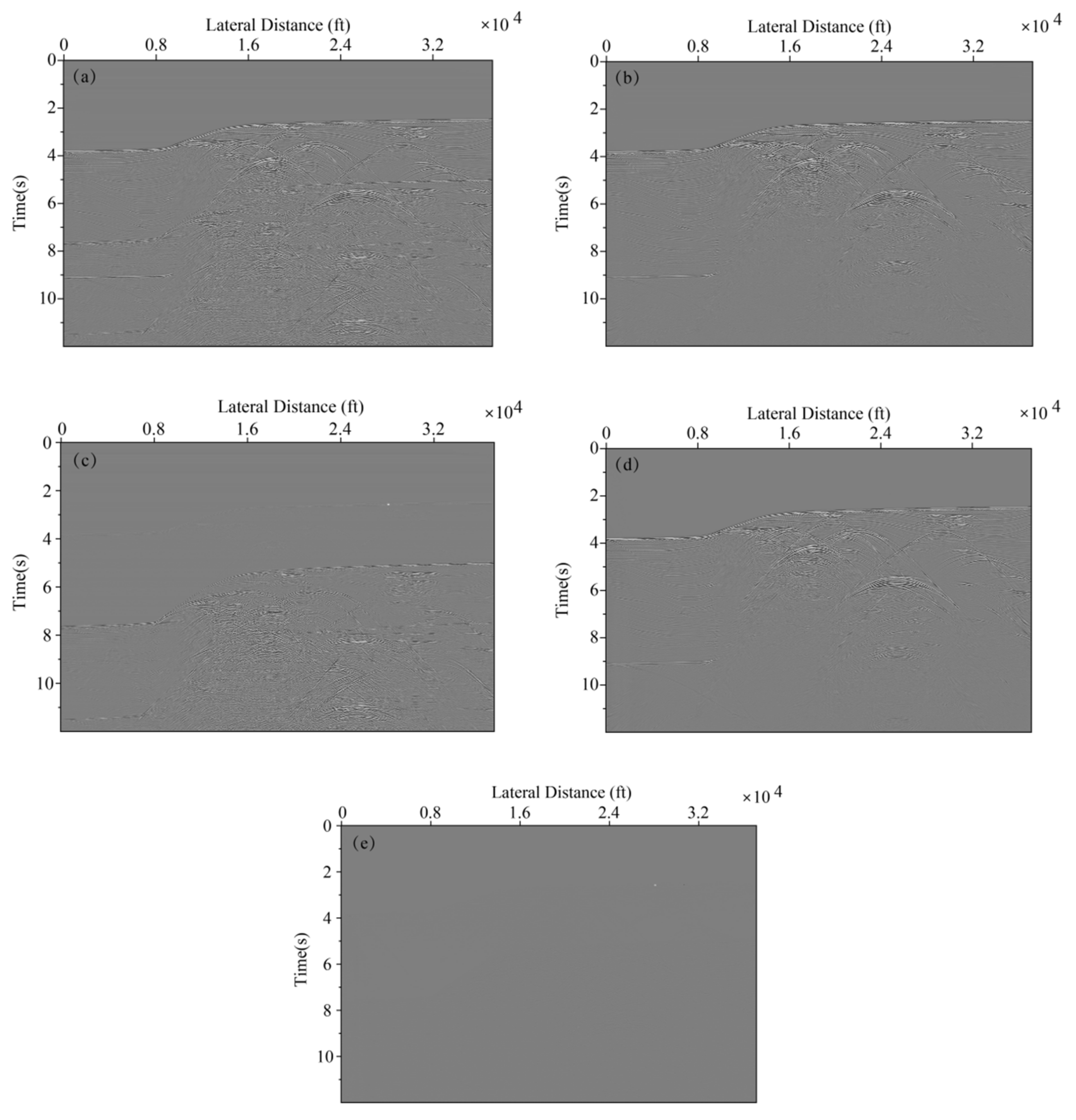
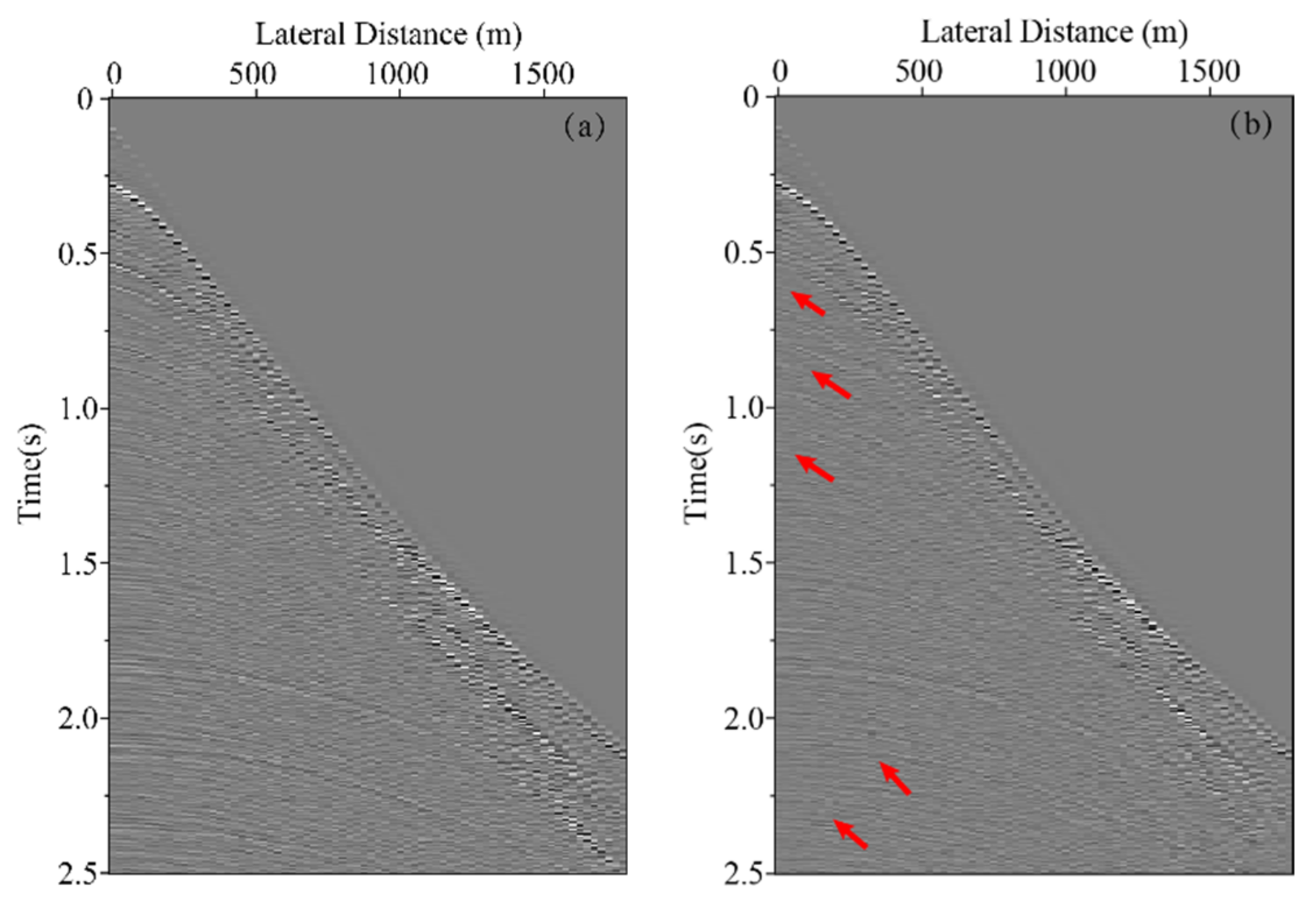
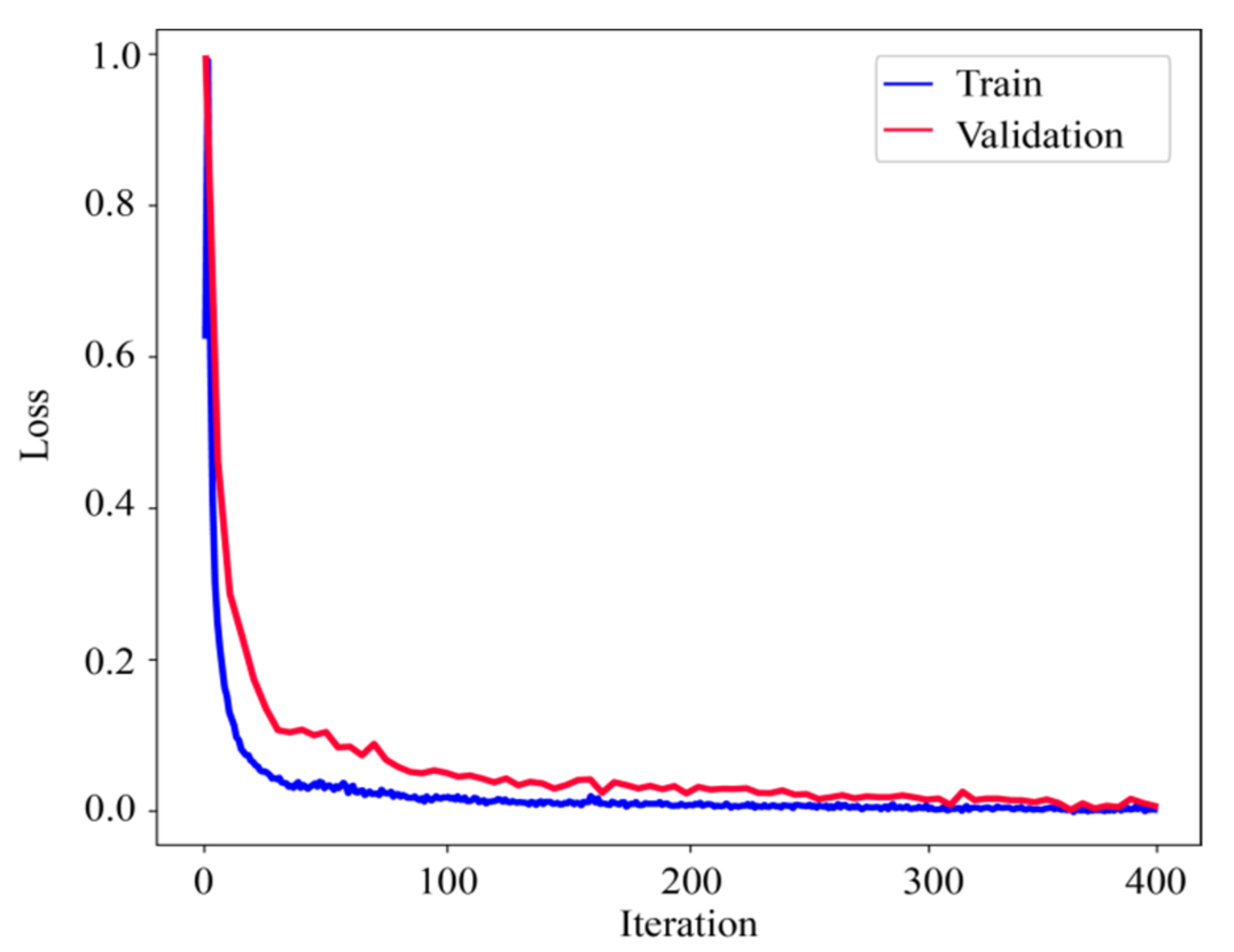
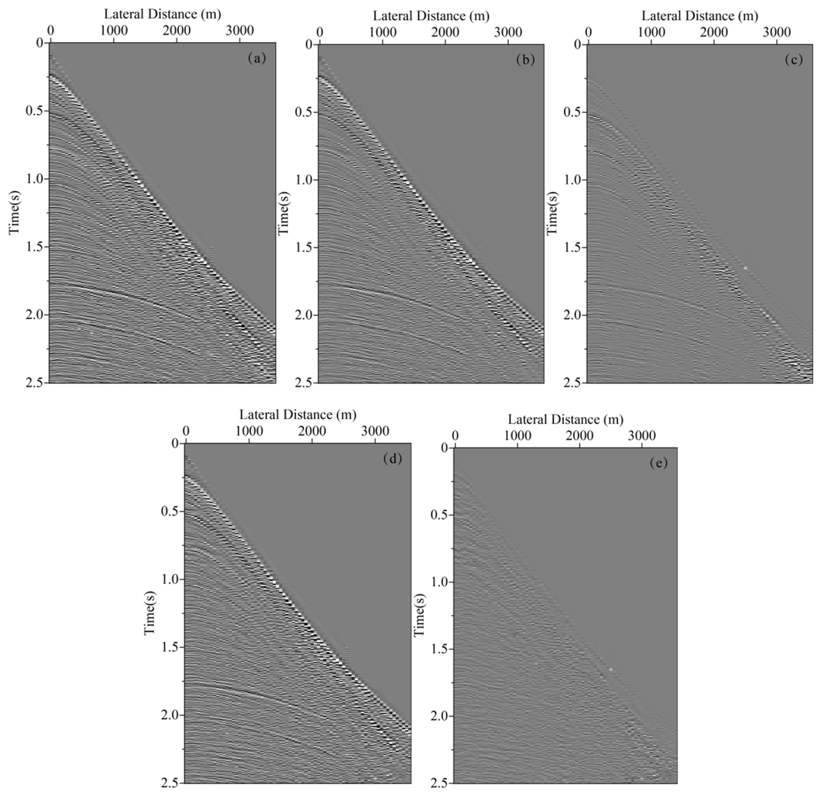
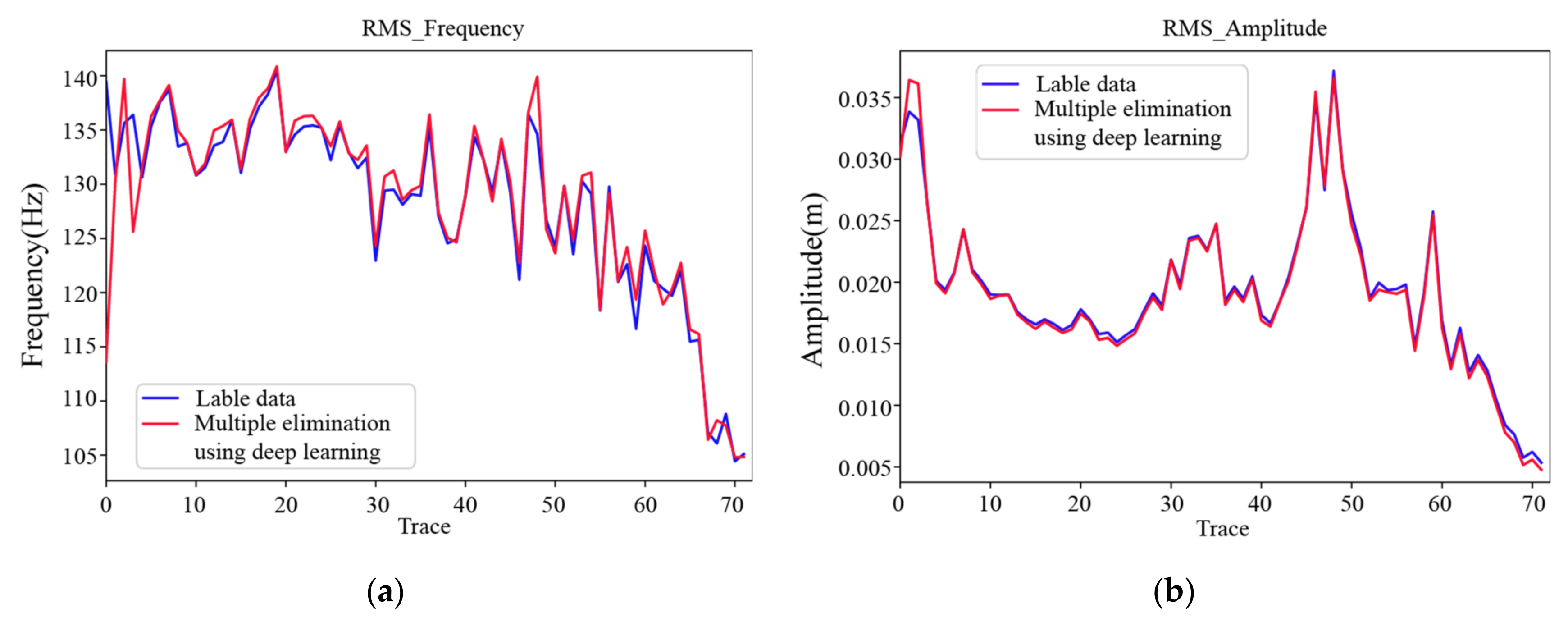
We extract a 2D seismic line which is 72 shot records each containing 72 traces from 3D seismic data to better illustrate the practicability of the multiple elimination method using deep learning. The shot records without multiples are obtained via the multiple suppression method based on inversion as lab data. The sampling interval of sources and receivers is 50 m, the time samples per trace is 626 and the time sampling interval is 0.004 s. We select 20 shot records as the training set in field data for network training in Figure 16, and other shot records are used as the test set. Multiples are eliminated as indicated by the red arrows. The network configuration is the same as the previous one, with 400 epochs. Figure 17 displays loss function for the network model training using the training data sets. Figure 18a illustrates the shot record with multiples and Figure 18d depicts the shot record without multiples. Figure 18b presents the shot record with multiple elimination using deep learning. Figure 18c presents the difference between Figure 18a,b. Figure 18e presents that the residual between seismic data after multiple elimination using the trained network and the label data is small, the average correlation of the test set is greater than 93.58%. Figure 19 sketches attribute analysis with multiple elimination using deep learning. Root mean square frequency analysis and Root mean square amplitude analysis of seismic data that multiple eliminated using deep learning in Figure 18b,d are presented in Figure 19a,b, respectively. The difference of root mean square frequency and root mean square amplitude between lab and predicted data is extremely small, suggesting the trained network can eliminate multiples in field data effectively with high coincidence. In addition, to test the generalization ability of the network better, we choose another shot record that is far away from the range of the 72 shot records for multiple elimination, the result are shown in Figure 20.
4. Discussion
In the data test part, the method is verified using two sets of synthetic data and one set of field data. Sigsbee2B model data mainly include surface-related multiples, synclinal model data mainly include internal multiples, and field data include both surface-related multiples and internal multiples. Compared with surface-related multiples in marine data, the energy of internal multiples on land is weaker but internal multiples always generate a hazy and occasionally strong interference pattern [45]. The NMO difference between internal multiples and primaries is also smaller [46], leading to more difficulties in eliminating internal multiples in Figure 13. We train the neural network according to the characteristics of two model data to ensure that excellent results can be achieved in surface-related multiple and internal multiple elimination using deep learning. Two different neural network models are obtained to eliminate surface-related multiples and internal multiples. In field data examples, surface-related multiples and internal multiples are eliminated to obtain label data. Therefore, the neural network trained with field data can eliminate surface-related multiples and internal multiples simultaneously.
Based on the neural network framework, it is essential to collect a large number of representative labeled data to obtain a good neural network. When the training set is too small or unrepresentative, the neural network model cannot capture the data characteristics in the learning process, resulting in poor generalization ability of the neural network model. For example, when testing sigsbee2B model data and synclinal model data, if we only choose the first 10 shot records of each model for neural network model training, the highest average correlation of test set results can only reach 90%. However, if shot records are chosen from sigsbee2B model data and synclinal model data which are 20 and 30 pairs of shots respectively for network training, the average correlation of each test set results can reach over 96%.
Field data are characterized by more intricacies compared to synthetic data. Field data often have the problems of absorption attenuation, anisotropy, irregular random scattering, and noise band limit. Moreover, the corresponding source wavelet is spatially variable, making the multiple elimination using neural networks more challenging. If field data are directly placed into the trained neural network model which uses synthetic data, the correlation between the prediction results and field data is extremely low, reaching 45%; such a low correlation cannot effectively eliminate multiples. Therefore, the corresponding neural network model needs to be retrained with field data. In the test part of field data, we choose 20 shot records as the training set in field data. The average correlation of each test set reaches more than 93%, suggesting excellent practicability of the network.
It is worth noting that we choose another shot record that is far away from the range of the 72 shot records for multiple elimination to test the generalization ability of the field data training network model and the correlation of test results reaches 87% (see Figure 20). Such results undoubtedly provide us more confidence in the network model for training larger datasets. It illustrates that if a small number of datasets that can reflect the characteristics of the seismic work area are selected for network model training, the purpose of eliminating multiples in the entire seismic area can be achieved. Our computer configuration is GPU 4*NVIDIA RTX2080TI 11G for the Sigsbee2B velocity model; training time per one batch of size 32 traces is 0.25 s, full model (20 pairs of shot records) training time with batch size 32 is 3:49:45 h, and all seismic data prediction time with batch size 348 is 2:14 min. Under the same influencing factors, SRME usually takes 25:47 min to predict and 37:42:33 h to subtract all Sigsbee2B seismic data. The adaptive subtraction method is l1/l2 method. Compared with SRME, the prediction time of the trained network model can be ignored. If the training set preparation time is not considered, the sum of full model training time and prediction time is also less than SRME. Therefore, using the trained network model to eliminate multiples, the calculation efficiency will be greatly improved, particularly for massive 3D seismic data. Moreover, in an ideal state, the trained network can also be applied to multiple elimination in other seismic areas directly or through the transfer learning method [47,48].
5. Conclusions
The multiple elimination method using deep learning adopted in this paper is completely data-driven without any prior information. The only requirement of the method is to input few seismic data with and without multiples for neural network training, then it applies the trained neural network to other seismic data to remove multiples. The test of synthetic data and field data indicates that the trained network can effectively distinguish primaries and multiples in seismic data, produce seismic data without multiples successfully, and the residual energy of multiples is very small. In addition, compared with the traditional multiple elimination methods, the prediction time of the trained network model can be ignored, which proving that the trained network has generalization ability and high calculation efficiency. It can be used in large-scale seismic data computation, particularly for massive 3D seismic data. However, the network architecture cannot completely solve the problem of fewer training samples. Therefore, we can study semi-supervised learning to better solve practical problems in the next step.
Author Contributions
Conceptualization, P.B. and Y.S.; methodology, P.B.; software, P.B. and X.G.; validation, P.B., Y.S. and W.W.; formal analysis, P.B. and Y.S.; investigation, P.B.; resources, Y.S.; data curation, P.B.; writing—original draft preparation, P.B.; writing—review and editing, P.B., Y.S. and X.G.; visualization, P.B. and Y.S.; supervision, J.X.; project administration, Y.S. and W.W.; funding acquisition, Y.S. and J.X. All authors have read and agreed to the published version of the manuscript.
Funding
This research was funded by the National Natural Science Foundation of China (Grant Nos. 41930431 and 41974116) and Petroleum Science and Technology Innovation Foundation of China (Grant Nos. 2019D-5007-0301).
Institutional Review Board Statement
Not applicable.
Informed Consent Statement
Not applicable.
Data Availability Statement
Not applicable.
Conflicts of Interest
The authors declare no conflict of interest.
References
- Taner, M.T. Long period sea-floor multiples and their suppression. Geophys. Prospect. 1980, 28, 30–48. [Google Scholar] [CrossRef]
- Hampson, D. Inverse Velocity Stacking for Multiple Elimination. In SEG Technical Program Expanded Abstracts; Society of Exploration Geophysicists: Houston, TX, USA, 1986; pp. 422–424. [Google Scholar] [CrossRef]
- Amundsen, L.; Ikelle, L.T.; Berg, L.E. Multidimensional signature deconvolution and free-surface multiple elimination of marine multicomponent ocean-bottom seismic data. Geophysics 2001, 66, 1594–1604. [Google Scholar] [CrossRef]
- Majdanski, M.; Kostov, C.; Kragh, E.; Moore, I.; Thompson, M.; Mispel, J. Attenuation of free-surface multiples by up/down deconvolution for marine towed-streamer data. Geophysics 2011, 76, 129–138. [Google Scholar] [CrossRef]
- Berkhout, A.J.; Verschuur, D.J. Estimation of multiple scattering by iterative inversion; Part 1, Theoretical consideration. Geophysics 1997, 62, 1586–1595. [Google Scholar] [CrossRef]
- Van Groenestijn, G.J.A.; Verschuur, D.J. Estimating primaries by sparse inversion and application to near-offset data reconstruction. Geophysics 2009, 74, A23–A28. [Google Scholar] [CrossRef] [Green Version]
- Ypma, F.H.C.; Verschuur, D.J. Estimating primaries by sparse inversion, a generalized approach. Geophys. Prospect. 2013, 61, 94–108. [Google Scholar] [CrossRef]
- Lin, T.; Herrmann, F.J. Robust estimation of primaries by sparse inversion via one-norm minimization. Geophysics 2013, 78, R133–R150. [Google Scholar] [CrossRef]
- Weglein, A.B.; Araújo, F.V.; Carvalho, P.M.; Stolt, R.H.; Matson, K.H.; Coates, R.T.; Corrigan, D.; Foster, D.J.; Shaw, S.A.; Zhang, H. Inverse scattering series and seismic exploration. Inverse Probl. 2003, 19, R27–R83. [Google Scholar] [CrossRef]
- Weglein, A.B.; Gasparotto, F.A.; Carvalho, P.M.; Stolt, R.H. An inverse-scattering series method for attenuating multiples in seismic reflection data. Geophysics 1997, 62, 1975–1989. [Google Scholar] [CrossRef]
- Jin, D.; Chang, X.; Liu, Y. Algorithm improvement and strategy of internal multiples prediction based on inverse scattering series method. Chin. J. Geophys. 2008, 51, 1209–1217. (In Chinese) [Google Scholar] [CrossRef]
- Berkhout, A.J.; Verschuur, D.J. Removal of internal multiples with the common-focus-point (CFP) approach: Part 1—Explanation of the theory. Geophysics 2005, 70, V45–V60. [Google Scholar] [CrossRef] [Green Version]
- Slob, E.; Wapenaar, K.; Broggini, F.; Snieder, R. Seismic reflector imaging using internal multiples with Marchenko-type equations. Geophysics 2014, 79, S63–S76. [Google Scholar] [CrossRef] [Green Version]
- Meles, G.A.; Löer, K.; Ravasi, M.; Curtis, A.; da Costa Filho, C.A. Internal multiple prediction and removal using marchenko autofocusing and seismic interferometry. Geophysics 2015, 80, A7–A11. [Google Scholar] [CrossRef] [Green Version]
- Thorbecke, J.; Zhang, L.; Wapenaa, K.; Slob, E. Implementation of the Marchenko Multiple Elimination algorithm. Geophysics 2020, 86, F9–F23. [Google Scholar] [CrossRef]
- Thorbecke, J.; Slob, E.; Brackenhoff, J.; van der Neut, J.; Wapenaar, K. Implementation of the Marchenko method. Geophysics 2017, 82, WB29–WB45. [Google Scholar] [CrossRef] [Green Version]
- Zhang, L.; Slob, E. A field data example of Marchenko multiple elimination. Geophysics 2020, 85, S65–S70. [Google Scholar] [CrossRef] [Green Version]
- IJsseldijk, J.; Wapenaar, K. Adaptation of the iterative Marchenko scheme for imperfectly sampled data. Geophys. J. Int. 2020, 224, 326–336. [Google Scholar] [CrossRef]
- Hinton, G.E.; Srivastava, N.; Krizhevsky, A.; Sutskever, I.; Salakhutdinov, R.R. Improving neural networks by preventing co-adaptation of feature detectors. Comput. Sci. 2012, 3, 212–223. [Google Scholar] [CrossRef]
- Ross, C.P.; Cole, D.M. A comparison of popular neural network facies-classification schemes. Lead. Edge 2017, 36, 340–349. [Google Scholar] [CrossRef]
- Xiong, W.; Ji, X.; Ma, Y.; Wang, Y.; Nasher, M.A.; Mustafa, N.A.; Luo, Y. Seismic fault detection with convolutional neural network. Geophysics 2018, 83, A23–A28. [Google Scholar] [CrossRef]
- Araya-Polo, M.; Jennings, J.; Adler, A.; Dahlke, T. Deep-learning tomography. Lead. Edge 2018, 37, 58–66. [Google Scholar] [CrossRef]
- Das, V.; Pollack, A.; Wollner, U.; Mukerji, T. Convolutional neural network for seismic impedance inversion. Geophysics 2019, 84, R869–R880. [Google Scholar] [CrossRef]
- Liu, L.; Fu, L.; Zhang, M. Deep-seismic-prior-based reconstruction of seismic data using convolutional neural networks. Geophysics 2021, 86, V131–V142. [Google Scholar] [CrossRef]
- Yu, J.; Wu, B. Attention and Hybrid Loss Guided Deep Learning for Consecutively Missing Seismic Data Reconstruction. IEEE Trans. Geosci. Remote Sens. 2022, 60, 1–8. [Google Scholar] [CrossRef]
- Wu, B.; Meng, D.; Zhao, H. Semi-supervised Learning for Seismic Impedance Inversion Using Generative Adversarial Networks. Remote Sens. 2021, 13, 909. [Google Scholar] [CrossRef]
- Siahkoohi, A.; Verschuur, D.J.; Herrmann, F.J. Surface-related multiple elimination with deep learning. In SEG Technical Program Expanded Abstracts; Society of Exploration Geophysicists: Houston, TX, USA, 2019; pp. 4629–4634. [Google Scholar] [CrossRef] [Green Version]
- Yu, S.; Ma, J.; Wang, W. Deep learning for denoising. Geophysics 2019, 84, V333–V350. [Google Scholar] [CrossRef]
- Qu, S.; Verschuur, E.; Zhang, D.; Chen, Y. Training deep networks with only synthetic data: Deep-learning-based near-offset reconstruction for closed-loop surface-related multiple estimation on shallow-water field data. Geophysics 2021, 86, A39. [Google Scholar] [CrossRef]
- Vrolijk, J.W.; Blacquière, G. Source deghosting of coarsely-sampled common-receiver data using a convolutional neural network. Geophysics 2021, 86, V185–V196. [Google Scholar] [CrossRef]
- Song, H.; Mao, W.; Tang, H. Applicatio of deep neural networks for multiples attenuation. Chin. J. Geophys. 2021, 64, 2795–2808. (In Chinese) [Google Scholar] [CrossRef]
- Hinton, G.E.; Salakhutdinov, R.R. Reducing the Dimensionality of Data with Neural Networks. Science 2006, 313, 504–507. [Google Scholar] [CrossRef] [Green Version]
- Ronneberger, O.; Fischer, P.; Brox, T. U-Net: Convolutional Networks for Biomedical Image Segmentation; Springer: Cham, Switzerland, 2015. [Google Scholar] [CrossRef]
- Zhang, L.; Slob, E. Free-surface and internal multiple elimination in one step without adaptive subtraction. Geophysics 2019, 84, A7–A11. [Google Scholar] [CrossRef]
- Bao, P.; Wang, X.; Xie, J.; Wang, W.; Shi, Y.; Xu, J.; Yang, Y. Internal multiple suppression method based on iterative inversion. Chin. J. Geophys. 2021, 64, 2061–2072. (In Chinese) [Google Scholar] [CrossRef]
- Quan, T.M.; Hildebrand, D.G.C.; Jeong, W.K. Fusionnet: A deep fully residual convolutional neural network for image segmentation in connectomics. arXiv 2016, arXiv:1612.05360. [Google Scholar] [CrossRef]
- Zhang, W.; Gao, J.; Jiang, X.; Sun, W. Consistent Least-Squares Reverse Time Migration Using Convolutional Neural Networks. IEEE Trans. Geosci. Remote Sens. 2021, 60, 1–19. [Google Scholar] [CrossRef]
- Saad, O.M.; Chen, Y. Deep denoising autoencoder for seismic random noise attenuation. Geophysics 2020, 85, V367. [Google Scholar] [CrossRef]
- Khudorozhkov, R.; Illarionov, E.; Broilovskiy, A.; Kalashnikov, N.; Podvyaznikov, D.; Arefina, A.; Kuvaev, A. SeismicPro Library for Seismic Data Processing and ML Models Training and Inference. 2019. Available online: https://github.com/gazprom-neft/SeismicPro (accessed on 11 April 2022).
- Krizhevsky, A.; Sutskever, I.; Hinton, G.E. ImageNet classification with deep convolutional neural networks. Commun. ACM 2017, 60, 84–90. [Google Scholar] [CrossRef]
- Clevert, D.-A.; Unterthiner, T.; Hochreiter, S. Fast and accurate deep network learning by exponential linear units (ELUS). In Proceedings of the ICLR (Poster), San Juan, Puerto Rico, 2–4 May 2016. [Google Scholar] [CrossRef]
- Girshick, R. Fast R-CNN. In Proceedings of the 2015 IEEE International Conference on Computer Vision (ICCV), Santiago, Chile, 7–13 December 2015; pp. 1440–1448. [Google Scholar]
- Kingma, D.; Ba, J. Adam: A Method for Stochastic Optimization. In Proceedings of the 3rd International Conference for Learning Representations, San Diego, CA, USA, 7–9 May 2015. [Google Scholar] [CrossRef]
- Bengio, Y. Practical Recommendations for Gradient-Based Training of Deep Architectures; Springer: Berlin/Heidelberg, Germany, 2012. [Google Scholar] [CrossRef] [Green Version]
- Staring, M.; Dukalski, M.; Belonosov, M.; Baardman, R.H.; Yoo, J.; Hegge, R.F.; van Borselen, R.; Wapenaar, K. Robust estimation of primaries by sparse inversion and Marchenko equation-based workflow for multiple suppression in the case of a shallow water layer and a complex overburden: A 2D case study in the Arabian Gulf. Geophysics 2021, 86, Q15–Q25. [Google Scholar] [CrossRef]
- Jakubowicz, H. Wave equation prediction and suppression of interbed multiples. In SEG Technical Program Expanded Abstracts; Society of Exploration Geophysicists: New Orleans, LA, USA, 1998; pp. 1527–1530. [Google Scholar] [CrossRef]
- Yosinski, J.; Clune, J.; Bengio, Y.; Lipson, H. How transferable are features in deep neural networks? In Proceedings of the 27th International Conference on Neural Information Processing Systems, Cambridge, MA, USA, 8 December 2014; pp. 3320–3328. [Google Scholar] [CrossRef]
- Wu, B.; Meng, D.; Wang, L.; Liu, N.; Wang, Y. Seismic Impedance Inversion Using Fully Convolutional Residual Network and Transfer Learning. IEEE Geosci. Remote Sens. Lett. 2020, 17, 2140–2144. [Google Scholar] [CrossRef]
Figure 1.
Sketch of a deep U-net architecture.

Figure 2.
Activation functions (a) and Loss functions (b). For (a), is or ; for (b) is , or .

Figure 3.
Selected parameters (the number of filters) for U-net architecture.

Figure 4.
Sigsbee2B velocity model.

Figure 5.
Partial training data set pairs. (a) Input shot record with primaries and surface-related multiples. (b) Input shot data without surface-related multiples.
Figure 5.
Partial training data set pairs. (a) Input shot record with primaries and surface-related multiples. (b) Input shot data without surface-related multiples.

Figure 6.
The loss function for training the network model using the training data sets in the Sigsbee2B model data.
Figure 6.
The loss function for training the network model using the training data sets in the Sigsbee2B model data.

Figure 7.
Shot record with surface-related multiple elimination using deep learning. (a) The 10th shot record with surface-related multiples. (b) The 150th shot record with surface-related multiples. (c) The 310th shot record with surface-related multiples. (d) The 10th shot record without surface-related multiples. (e) The 150th shot record without surface-related multiples. (f) 310th shot record without surface-related multiples. (g) The 10th shot record without surface-related multiple elimination using deep learning. (h) The 150th shot record without surface-related multiple elimination using deep learning. (i) The 310th shot record without surface-related multiple elimination using deep learning. (j) The difference between (d) and (g). (k) The difference between (e) and (h). (l) The difference between (f) and (i).


Figure 8.
Zero-offset data with surface-related multiple elimination using deep learning. (a) Original zero-offset data with surface-related multiples. (b) Result after using deep learning. (c) The predicted internal multiples (the difference between (a) and (b)). (d) Original zero-offset data without surface-related multiples. (e) The difference between (b) and (d).

Figure 9.
A comparison of 37th traces from Figure 7a,d,g.
Figure 9.
A comparison of 37th traces from Figure 7a,d,g.

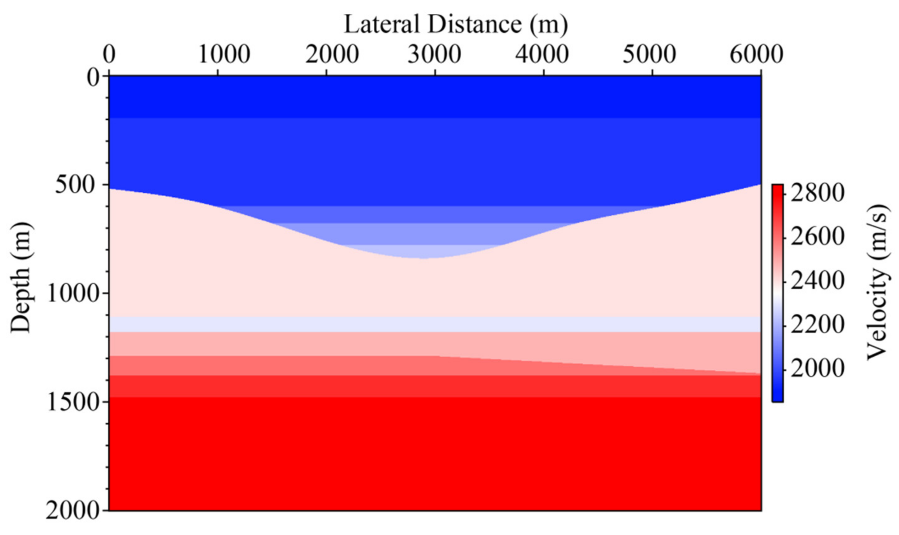
Figure 10.
Syncline velocity model.

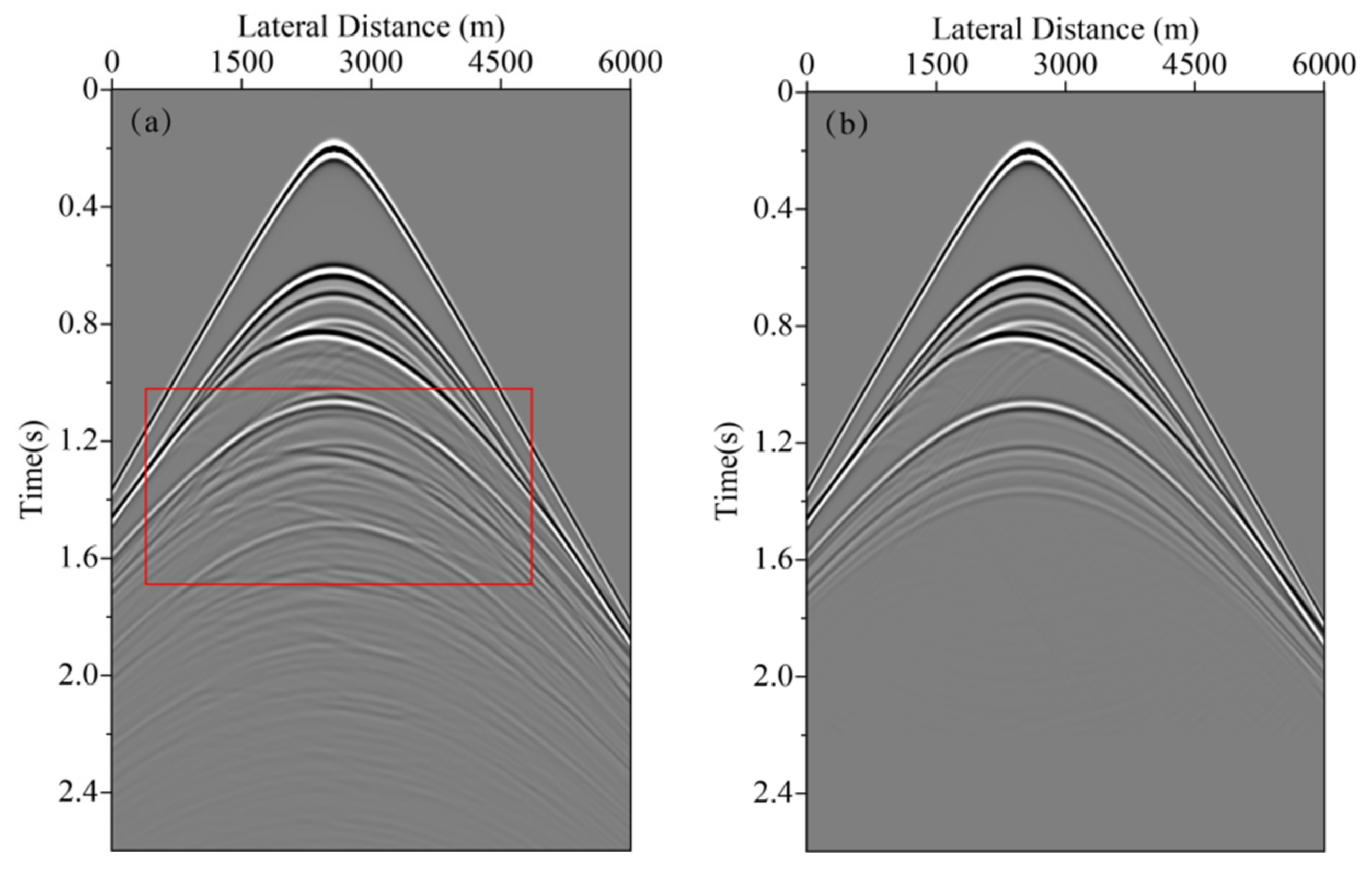
Figure 11.
Partially training data set pairs. (a) Input shot record with primaries and internal multiples. (b) Input shot data without internal multiples.
Figure 11.
Partially training data set pairs. (a) Input shot record with primaries and internal multiples. (b) Input shot data without internal multiples.

Figure 12.
The loss function for training the network model using the training data sets in the Syncline model data.
Figure 12.
The loss function for training the network model using the training data sets in the Syncline model data.

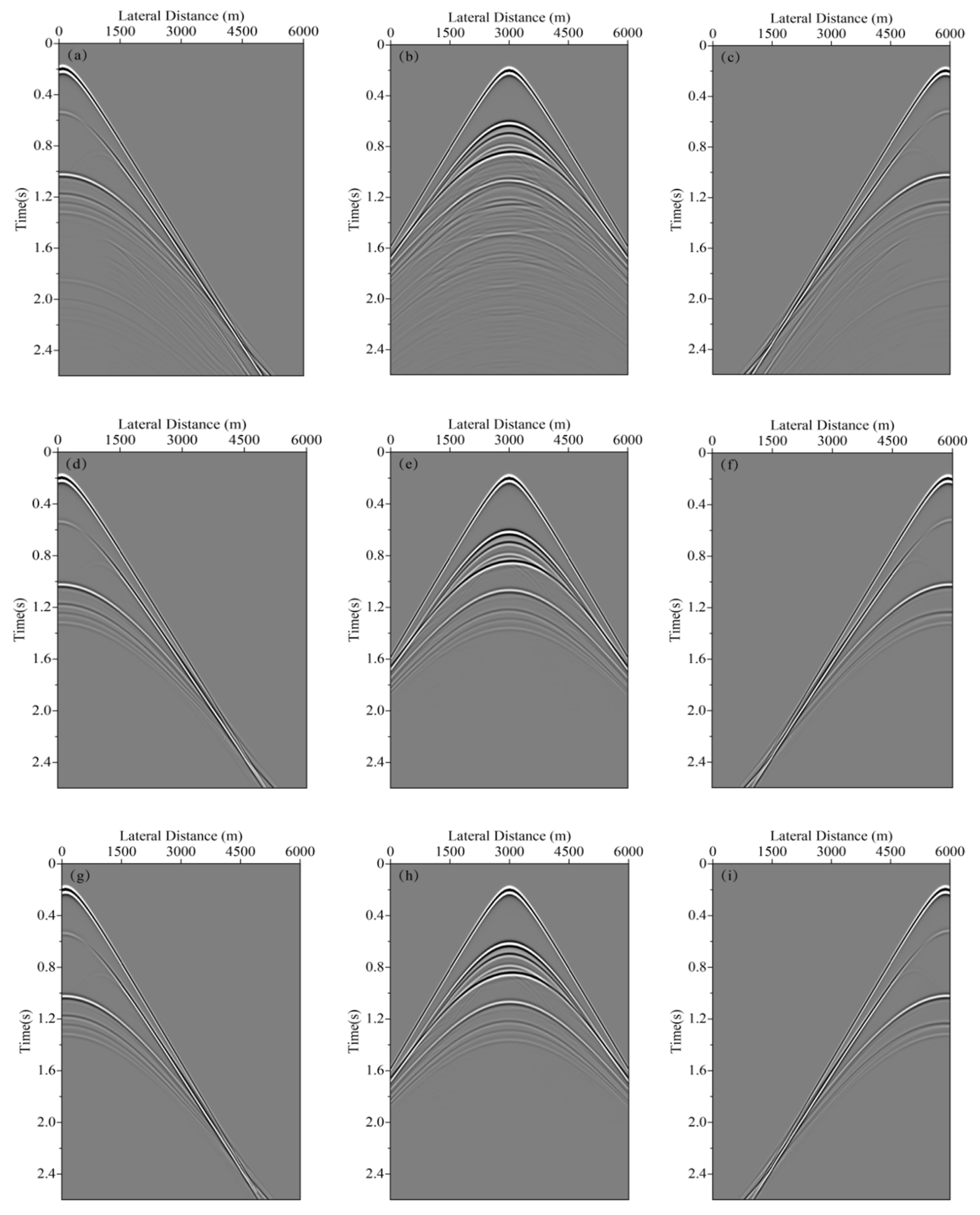
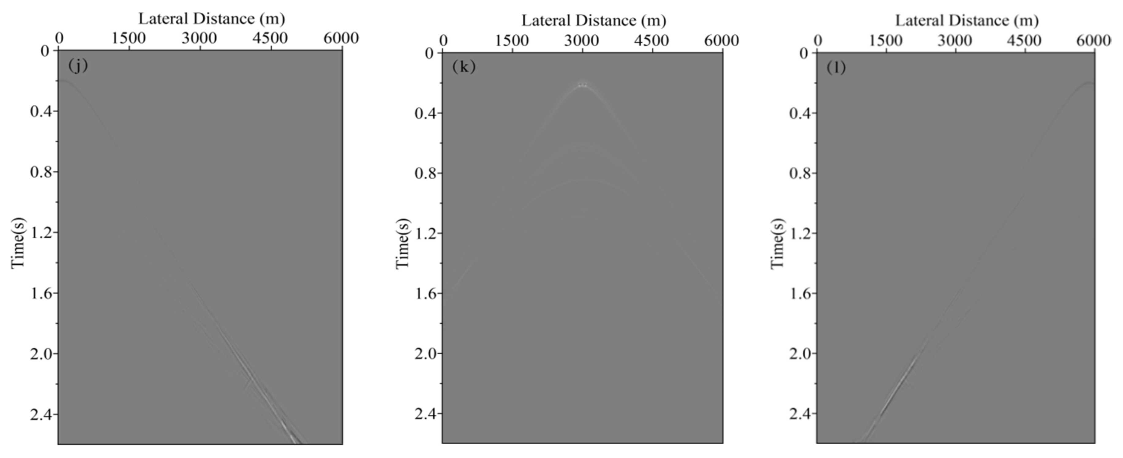
Figure 13.
Shot record with internal multiple elimination using deep learning. (a) The 10th shot record with internal multiples. (b) The 300th shot record with internal multiples. (c) The 590th shot record with internal multiples. (d) The 10th shot record without internal multiples. (e) 300th shot record without internal multiples. (f) The 590th shot record without internal multiples. (g) The 10th shot record with internal multiple elimination using deep learning. (h) The 300th shot record with internal multiple elimination using deep learning. (i) The 590th shot record with internal multiple elimination using deep learning. (j) The difference between (d) and (g). (k)The difference between (e) and (h). (l) The difference between (f) and (i).


Figure 14.
Zero-offset data with internal multiple elimination using deep learning. (a) Original zero-offset data with internal multiples. (b) Result after using deep learning. (c) The predicted internal multiples (the difference between ((a) and (b)). (d) Original zero-offset data without internal multiples. (e) The difference between (b) and (d).

Figure 15.
A comparison of 300th traces from Figure 13b,e,h.
Figure 15.
A comparison of 300th traces from Figure 13b,e,h.

Figure 16.
Partial training data set pairs. (a) Input shot record with primaries and multiples. (b) Input shot record without multiples.
Figure 16.
Partial training data set pairs. (a) Input shot record with primaries and multiples. (b) Input shot record without multiples.

Figure 17.
The loss function for training the network model using the training data sets in the field data.
Figure 17.
The loss function for training the network model using the training data sets in the field data.

Figure 18.
Shot record with multiple elimination using deep learning. (a) Shot record with multiples. (b) Shot record with multiple elimination using deep learning. (c) The predicted multiples (the difference between ((a) and b)). (d) Shot record without multiples. (e) The difference between (b) and (d).

Figure 19.
Attribute analysis with multiple elimination using deep learning. (a) Root mean square frequency analysis of seismic data with multiple elimination using deep learning in Figure 18b,d. (b) Root mean square amplitude analysis of seismic data with multiple elimination using deep learning in Figure 18b,d.

Figure 20.
Shot record with multiple elimination using deep learning. (a) Shot record with multiples. (b) Shot record with multiple elimination using deep learning. (c) The predicted multiples (the difference between ((a) and (b)). (d) Shot record without multiples. (e) The difference between (b) and (d).

Publisher’s Note: MDPI stays neutral with regard to jurisdictional claims in published maps and institutional affiliations. |
© 2022 by the authors. Licensee MDPI, Basel, Switzerland. This article is an open access article distributed under the terms and conditions of the Creative Commons Attribution (CC BY) license (https://creativecommons.org/licenses/by/4.0/).
Share and Cite
MDPI and ACS Style
Bao, P.; Shi, Y.; Wang, W.; Xu, J.; Guo, X. Surface-Related and Internal Multiple Elimination Using Deep Learning. Energies 2022, 15, 3883. https://doi.org/10.3390/en15113883
AMA Style
Bao P, Shi Y, Wang W, Xu J, Guo X. Surface-Related and Internal Multiple Elimination Using Deep Learning. Energies. 2022; 15(11):3883. https://doi.org/10.3390/en15113883
Chicago/Turabian StyleBao, Peinan, Ying Shi, Weihong Wang, Jialiang Xu, and Xuebao Guo. 2022. "Surface-Related and Internal Multiple Elimination Using Deep Learning" Energies 15, no. 11: 3883. https://doi.org/10.3390/en15113883
Note that from the first issue of 2016, this journal uses article numbers instead of page numbers. See further details here.