Research on an Optimization Method for Injection-Production Parameters Based on an Improved Particle Swarm Optimization Algorithm

Abstract

The optimization of injection–production parameters is an important step in the design of gas injection development schemes, but there are many influencing factors and they are difficult to determine. To solve this problem, this paper optimizes injection-production parameters by combining an improved particle swarm optimization algorithm to study the relationship between injection-production parameters and the net present value. In the process of injection-production parameter optimization, the particle swarm optimization algorithm has shortcomings, such as being prone to fall into local extreme points and slow in convergence speed. Curve adaptive and simulated annealing particle swarm optimization algorithms are proposed to further improve the optimization ability of the particle swarm optimization algorithm. Taking the Tarim oil field as an example, in different stages, the production time, injection volume and flowing bottom hole pressure were used as input variables, and the optimal net present value was taken as the goal. The injection-production parameters were optimized by improving the particle swarm optimization algorithm. Compared with the particle swarm algorithm, the net present value of the improved scheme was increased by about 3.3%.

1. Introduction

With the deepening of development, the oil field will enter a high-water-cut stage. Due to the heterogeneity of the reservoir, the injection of the injected material in the reservoir is not balanced and the contradiction within the layer is prominent, which seriously influence the reservoir development effect. Some development contradictions are gradually exposed, such as the decline of oil production in the production cycle and the deterioration of the effect of measures, which restrict the production efficiency of oil wells and directly affect the net present value of oil fields. The quality of the injection-production development effect is mainly affected by a reservoir’s geological parameters and the injection-production parameters. To improve the development effect, injection-production optimization is implemented to increase oil production from oil wells.

In the process of injection-production development, the determination of the injection-production parameters of a well group has always been a difficult problem. Different injection-production parameters will have a significant impact on recovery [1]. During the development process, the influence of injection-production parameters is particularly prominent due to the heterogeneity of the reservoir itself and the large differences in the recovery factors of different well patterns. Since the optimization of injection-production schemes is a complex nonlinear dynamic optimization problem affected by multifactor interaction [2], at present, large-scale numerical simulation software is mainly used to determine optimal injection-production parameters through a simulation calculation at home and abroad. This numerical simulation software is complicated to operate due to the consideration of many factors, and the optimization efficiency is not good.

In recent years, many scholars have introduced mathematical and machine learning methods to optimize actual injection and extraction parameters. Common methods for determining injection-production parameters include numerical simulation [3,4,5] and various evolutionary algorithms, such as the genetic algorithm [6,7], the artificial bee colony algorithm [8], the particle swarm optimization (PSO) algorithm [9], etc., in order to obtain better injection-production parameters, and there is a certain reference significance. Zhang et al. [10] used numerical simulation methods to optimize single-well production, injection volume and oil production rate in the gas injection stage in the depletion stage. Wang et al. [11] established an optimization mathematical model based on the particle swarm optimization algorithm and took maximizing oil production as the goal to jointly optimize the well pattern and injection-production parameters. Wu et al. [12] took the net present value as the objective function and optimized injection-production parameters through the differential optimization algorithm. Yu et al. [13] used the response surface method to optimize injection-production parameters and obtained an optimal solution. Zhang et al. [14] considered the injection-production optimization model of binary composite flooding and solved it by using the optimal disturbance approximate gradient method.

However, the above methods also have their own limitations. The numerical simulation method has a good effect on the simulation of smaller models, but the simulation of larger models requires a substantial amount of computing time, so it is not convenient for field applications. Compared with the genetic algorithm, particle swarm optimization has an important feature: that is, particles have memory. The information sharing mechanism of particle swarm optimization is very different. In the genetic algorithm, chromosomes share information with each other, so the movement of the entire population is relatively uniform to the optimal area. In the particle swarm optimization algorithm, only the global best gives information to other particles, and there is no information sharing between particles. Each update is directed to the global optimal solution and is not affected by other particles. Compared with the genetic algorithm, the particle swarm algorithm has simpler rules, and in most cases all particles may converge to the optimal solution faster. Additionally, the particle swarm optimization algorithm has been well-applied in the solution of various complex petroleum engineering optimization problems due to the advantages of easy implementation, few setting parameters and a fast convergence speed [15].

It is precisely based on the above advantages that the innovation and performance of the particle swarm optimization algorithm have been continuously improved, and many achievements have been achieved. Zhang et al. [16] popularized the results of the strategy of the exponential decline of inertia weight, and proposed an adjustment strategy of inertia weight in order to reduce the number of times weight was calculated. Huang et al. [17] proposed the strategy of nonlinear decreasing inertia weight based on the sigmoid function, and made use of the characteristics of the sigmoid function to make the inertia weight decrease slowly in the early and late stage of the algorithm. Kordestani et al. [18] combined the idea of linear decreasing inertia weight with linear increasing inertia weight and proposed the strategy of adjusting inertia weight in the way of a symmetric triangle wave. Due to the oscillating change in the inertia weight, these two strategies effectively balance the global search ability and local search ability. Jiang et al. [19] proposed a strategy of adjusting the inertia weight in a sinusoidal manner. The inertia weight of the strategy increases from 0.4 to 0.9 in the form of a sinusoidal curve, and then decreases to 0.4 in the form of a sinusoidal curve. Li et al. [20] proposed a nonlinear decreasing strategy of inertia weight based on the inverse incomplete Γ function, which is close to an exponential decrease in the later stage, which can better achieve a balance between global search ability and local search ability. In this paper, the above ideas are used to optimize the injection-production parameters by improving the particle swarm algorithm.

In this paper, the program samples under different injection-production parameters are calculated by numerical simulation, and they are substituted into the neural network model for training to reduce the calculation time. Then, referring to the advantages of the particle swarm optimization algorithm, according to the calculation method for oil field benefit, the appropriate objective function is selected. The net present value is taken as the objective function, and the gas injection rate, water injection rate and flowing bottom hole pressure are taken as the constraints: a mathematical model for optimizing the injection-production scheme is established. The particle swarm optimization algorithm is used to optimize the injection-production parameters, and an improved particle swarm optimization algorithm is proposed for the model. The optimal solution of the model is further obtained, and the optimal injection-production plan is optimized. This method can guide the preparation of field development plans and realize the scientific management of deep gas injection reservoirs.

2. Basic Particle Swarm Optimization

Particle swarm optimization was proposed by Dr. Kennedy and Eberhart in 1995 [21]. It is widely used to solve constrained optimization problems. When solving multiobjective optimization problems, it is called multiobjective particle swarm optimization.

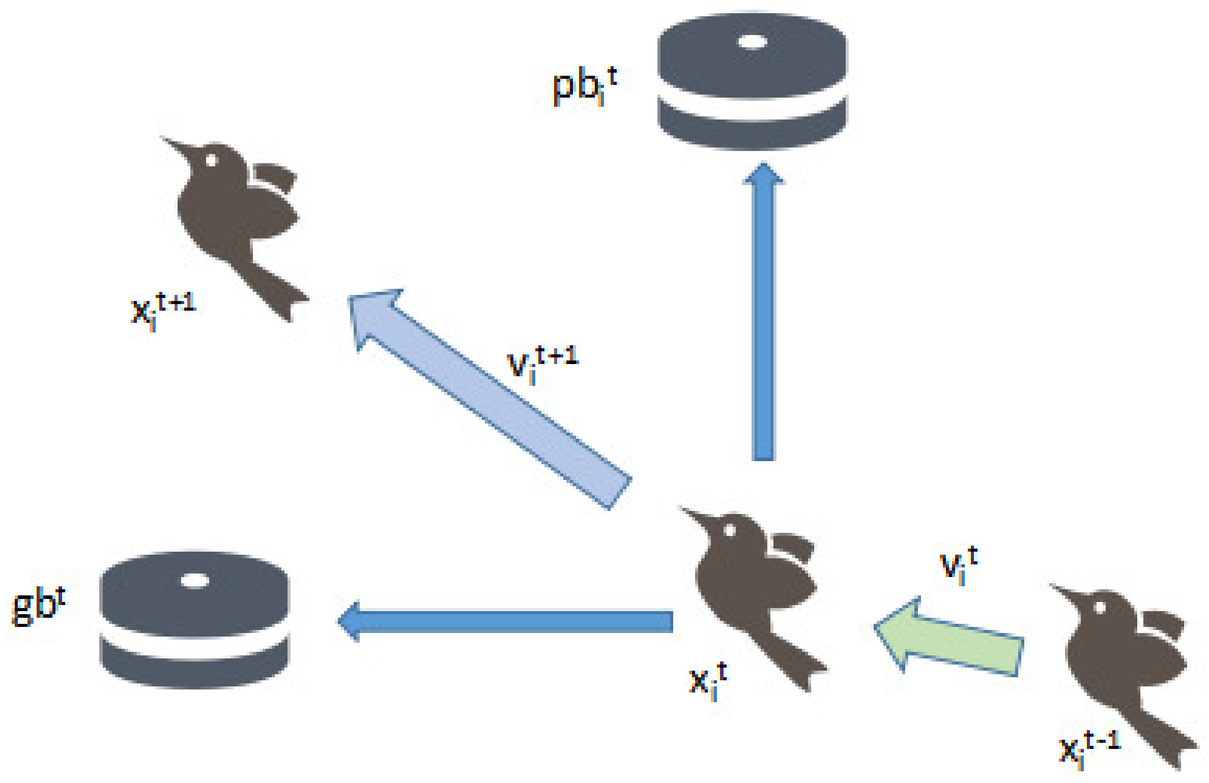
In the PSO algorithm, considering the individual positions or objects in the flock as the solution to an optimization problem, the information interaction among the individuals in the group and the optimal individual is used to guide the individuals in the whole group to converge toward the optimal individual of the group while maintaining their own diversity information. The optimal individual of the group converges, and the optimal solution is gradually found through continuous updating. The individuals in the flock are abstracted as “particles”, and their mass and volume are ignored. The topology structure determines that the “particles” are affected by the comprehensive influence of themselves and the group state information in each iteration. That is, the update mechanism of particles is obtained through the organic combination of the historical best position of the population and the best position of the individual, as shown in Figure 1. The velocity of the particle i at the next moment $v_i^{t+1}$ is jointly determined by the current velocity $v_i^t$, its own best position $p{b}_i^t$, and the global best position $g{b}^t$. The particle moves from the current position $x_i^t$ to the new position $x_i^{t+1}$ at the updated velocity [22]. With the continuous deepening of the iteration, the entire particle population, driven by the optimal solution, completes the search for the optimal solution in the decision space.

3. Optimization Model of Injection-Production Scheme

Different injection-production systems have a great impact on the actual development of oil fields, and the economic benefit index is usually used as the measurement standard. In this paper, according to the calculation method of oil field benefit, a mathematical model for the optimization of a reservoir injection-production scheme is established. In order to obtain optimal injection-production parameters, the net present value (NPV) is selected as the objective function, and the injection-production system is the parameter to be optimized.

• Objective Function;
  The optimization goal is to maximize the net present value. The objective function is established as the following:

  $$NPV=\sum _{k=1}^{Nt}[\frac{1}{{(1+b)}^k}(\sum _{i=1}^{Np}{r}_{gp}{q}_{gp}^{i,k}+\sum _{i=1}^{Np}{r}_{op}{q}_{op}^{i,k}-\sum _{i=1}^{Ng}{c}_{gi}{q}_{gi}^{i,k}-\sum _{i=1}^{Nw}{c}_{wi}{q}_{wi}^{i,k}-\sum _{i=1}^{Np}c{d}_{wp}{q}_{wp}^{i,k})],$$

  (1)

  where NPV is the function to be optimized, representing the net present value; b is the benchmark rate of return; $N_t$ is the calculation period of the project; k is the kth period; $N_p$, $N_g$ and $N_w$ are the number of production wells, the number of gas injection wells and the number of water injection wells, respectively; $r_{gp}{q}_{gp}$ is the sales revenue of natural gas; $r_{op}{q}_{op}$ is the sales revenue of oil; $c_{gi}{q}_{gi}$ is the cost of gas injection; $c_{wi}{q}_{wi}$ is the cost of water injection; and $c{d}_{wp}{q}_{wp}$ is the cost of water treatment.
• Data Composition;
  In order to make the paper easy to understand, we unify the parameter symbols. The parameters defined in the parameter table are all parameters related to injection-production.

  Table 1. Parameter declaration table.

  No.	Symbol	Comment
  1	t	Production time
  2	$q_g$	Injection volume of gas well
  3	$q_w$	Injection volume of water well
  4	p	Flowing bottom hole pressure of the production well
  5	S	Injection-production parameter matrix
  6	s	Numerical values on supplementary dimensions

  below is the parameter table of injection-production in the paper.
  In the process of gas injection development, unreasonable injection-production parameters will lead to low production, which will affect the ultimate recovery factor and economic benefits. Injection-production parameters are usually adjusted according to field experience and production conditions. In this paper, the injection-production scheme of multiple well patterns are considered in the simulation. Assuming that there are 15 types of well patterns, and that the kth well pattern has m gas injection wells, n water injection wells and o production wells, the injection-production parameter matrix of this well pattern is:

  $$S_k=[t_k,q_g^1,q_g^2,\dots ,q_g^m,q_w^1,q_w^2,\dots ,q_w^n,p^1,p^2,\dots ,p^o],$$

  (2)

  among them, $t_k$ represents the training production time, $q_g^i(i=1,2,\dots ,m)$ represents the injection volume of a gas well, $q_w^i(i=1,2,\dots ,n)$ represents the injection volume of a water well and $p^i(i=1,2,\dots ,o)$ represents the flowing bottom hole pressure of the production well.

  Table 2. An example of the value of injection-production parameters.

  t	${\mathit{q}}_{\mathit{g}}^1$	${\mathit{q}}_{\mathit{g}}^2$	${\mathit{q}}_{\mathit{g}}^3$	${\mathit{q}}_{\mathit{g}}^4$	${\mathit{q}}_{\mathit{w}}^1$	${\mathit{q}}_{\mathit{w}}^2$	${\mathit{p}}^1$	${\mathit{p}}^2$
  10	69,008	67	29	77,614	21	29	65	48
  10	49	35,773	62	32	126	37	16	129
  10	77,609	1008	70	27,614	53	22	32	83
  10	21,680	120	70,428	48,305	31	98	41	139

  below is an example of the injection-production parameters of a block in the Tarim oil field. The m mentioned above is four, and both n and o are two.
  Through observation, it can be found that there is a large difference in the order of magnitude in the data on gas injection, such as 69,008 and 67. This is because, in the actual production process, the gas wells may be converted into water wells. The abovementioned 69,008 corresponds to the data on gas injection, and 67 corresponds to the data on water injection. The two data units are different, resulting in a large difference in the order of magnitude. In order to separate the two data segments and ensure the accuracy of the prediction, the data are dimensionally aligned, and m parameters $s^i(i=1,2,\dots ,m)$ are added after the $m+$ first parameter of the injection-production parameter matrix $S_k$. When gas is injected into gas well one, $q_g^1$ corresponds to the injection volume and $s^1$ corresponds to zero; when gas well one is injected with water, $q_g^1$ corresponds to zero and $s^1$ corresponds to the injection volume. The input parameters under different production well patterns and different parameter combinations can be obtained, and their expressions are as follows:

  $$S_k=[t_k,q_g^1,q_g^2,\dots ,q_g^m,s^1,s^2,\dots ,s^m,q_w^1,q_w^2,\dots ,q_w^n,p^1,p^2,\dots ,p^o],$$

  (3)

  the following

  Table 3. An example of the dimension alignment of injection-production parameters.

  t	${\mathit{q}}_{\mathit{g}}^1$	${\mathit{q}}_{\mathit{g}}^2$	${\mathit{q}}_{\mathit{g}}^3$	${\mathit{q}}_{\mathit{g}}^4$	${\mathit{s}}^1$	${\mathit{s}}^2$	${\mathit{s}}^3$	${\mathit{s}}^4$	${\mathit{q}}_{\mathit{w}}^1$	${\mathit{q}}_{\mathit{w}}^2$	${\mathit{p}}^1$	${\mathit{p}}^2$
  10	69,008	0	0	77,614	0	67	29	0	21	29	65	48
  10	0	35,773	0	0	49	0	62	32	126	37	16	129
  10	77,609	1008	0	27,614	0	0	70	0	53	22	32	83
  10	21,680	0	70,428	48,305	0	120	0	0	31	98	41	139

  is the result of the abovementioned instance after dimension alignment: that is, the training data of the neural network.
  The flowing bottom hole pressure, injection volume and other factors are regarded as the main control factors of oil well productivity: that is, the data are preprocessed first, and then the processed data are used for training. The data and prediction model in this paper refer to reference [23], and the specific prediction process will not be described in detail here.
• The Restrictions.
  Gas injection speed:

  $$q_g^{min}\le q_g\le q_g^{max},$$

  (4)

  water injection rate:

  $$q_w^{min}\le q_w\le q_w^{max},$$

  (5)

  flowing bottom hole pressure of production well:

  $$p^{min}\le p\le p^{max},$$

  (6)
  The objective function Formula (1), and the constraints conditions Formulas (4)–(6), constitute the optimization model of the injection-production scheme. The model is a complex nonlinear optimization model with multiple variables and multiple constraints, which can be solved by the particle swarm optimization algorithm to obtain the maximum oil recovery and the best economic effect.

In addition, we performed a sensitivity analysis, and used correlation analysis to study the correlation between the gas injection rate, water injection rate, flowing bottom hole pressure of production wells and NPV, and used the p-value to indicate the strength of the correlation. The results of the analysis are shown in the

Table 4. Correlation analysis table.

Independent Variable	p-Value
Gas injection rate 1	0.016
Gas injection rate 2	0.017
Water injection rate 1	0.009
Water injection rate 2	0.008
Flowing bottom hole pressure 1	0.022
Flowing bottom hole pressure 2	0.009

. The specific analysis shows that some independent variables, such as the gas injection rate of gas injection wells one and two, have a correlation with the NPV, and that some independent variables, such as the water injection rate of water injection wells one and two, have a significant positive correlation with the NPV, thus proving the rationality of the experiment.

4. Particle Swarm Optimization Algorithm Based on Curve Adaptation (CAPSO)

In the standard PSO algorithm, the variable $w^t$ is the inertia weight in tth iterations. A larger inertia weight will lead to global exploration, while a smaller inertia weight will promote local exploration, and the current search area can be fine-tuned. The definition of $w^t$ is as follows:

$$w^t=w_{max}-(w_{max}-w_{min})\times \frac{iter}{iter\_max},$$

(7)

where $w_{max}$ and $w_{min}$ are the maximum inertia weight and minimum inertia weight, respectively; $iter$ is the number of iterations; and $iter\_max$ is the maximum number of iterations. The inertia weight parameter w of the particle swarm decreases with an increase in the number of iterations, which is conducive to the movement of particles near the target value, so that the optimal solution of the algorithm gradually converges to the target value. This is to control and balance the transition of PSO from exploration to development in the entire optimization process; therefore, the inertia weight parameter w is a very important control parameter in standard PSO, which has a significant impact on PSO performance. Parameter w in PSO adopts linear adaptive reduction and controls the exploration and development capabilities of PSO. However, the rapid decline of parameter w in the early stage of the calculation will lead to insufficient exploration in the early stage, resulting in the failure of PSO to search for the global optimum;; if the reduction in the late stage of the algorithm is too slow, the algorithm is not developed enough in the later stage, resulting in the failure of PSO to accurately search in the local area [24]. According to this phenomenon, parameter w adopts the processing method of curve adaptive adjustment, which can effectively solve the problem. Using an adaptive value method, the parameter w is expressed as follows:

$$w^t=(cos(\pi \times \frac{iter}{iter\_max})+w_{max})\times (w_{max}+w_{min})/2,$$

(8)

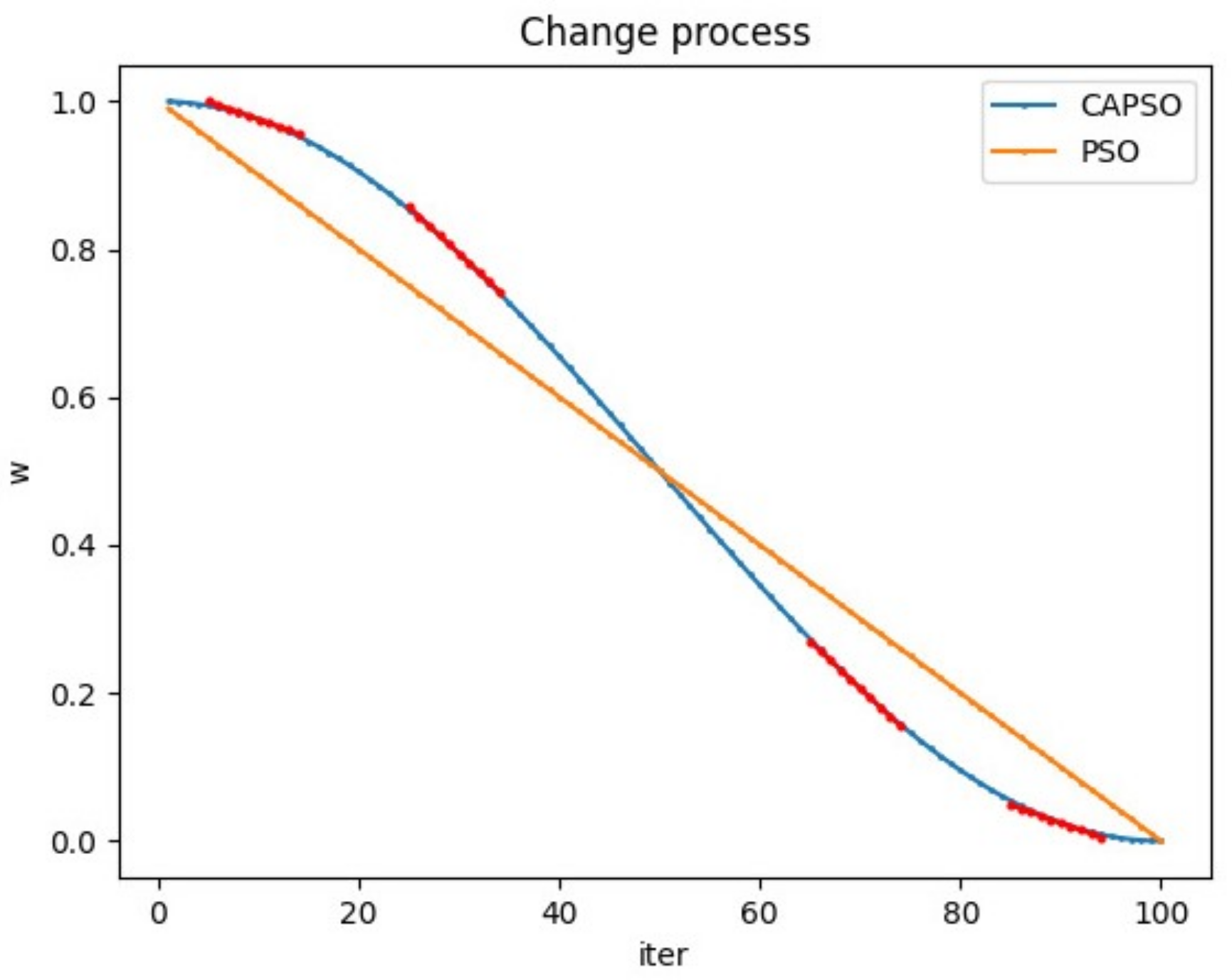
The cosine curve adaptive strategy is mainly used in the CAPSO proposed in this paper. Additionally, Formula (8) replaces the method of the linear adaptive updating parameter w in the particle swarm optimization algorithm (Formula (7)), thus forming a new CAPSO. The selection of parameter w is related to the search range of particles: it will affect the global and local search ability of the PSO algorithm, and the larger w is the stronger the global search ability is. The change curves of the two methods are shown in Figure 2, where the red line represents the decreasing rate of parameter w at different points in the CAPSO algorithm. The difference between curve adaptation and linear adaptation is the decreasing trend of parameter w. Linear adaptation reduces at the same speed; however, the cosine adaptive strategy is slow at the beginning and the end of the descent, which helps to enhance the global search ability of the particle at the beginning and the local search ability at the later stage. In addition, the value of parameter w is greater than the linear adaptation in the early cosine adaptation, which can expand the search and enhance the particle exploration ability; later cosine adaptation is less than linear adaptation, which can narrow the search for particles and improve particle swarm exploration capabilities.

5. Particle Swarm Optimization Algorithm Based on Curve Adaptation and Simulated Annealing

In the particle swarm optimization algorithm, the updating of the position of each particle is determined by its current position and the best position of all other particles [25]. Although the particle swarm optimization algorithm ensures that, in each iteration, the position with the best fitness value of all particles is saved as the global best position to guide the next position update of each particle, and its own best position parameter is retained to guide the position update of the current particle, there is no limit to the updated position of each particle and the updated position may become worse. Although the worse particle position will not affect the updating of the current particle position, it will lead to a slow convergence speed of the particle swarm optimization algorithm. Therefore, the quality of updating the particle position in each iteration is very important for the overall optimization and convergence speed of the particle swarm optimization algorithm. In order to improve the quality of the particle solution for each iteration, the simulated annealing algorithm is combined [26].

The simulated annealing algorithm was proposed by Metropolis et al. [27] in 1953, the basic idea being derived from the annealing process of solids. The algorithm is based on statistical physics, introduces the natural mechanism of the solid annealing process into the physical system and uses the Metropolis criterion to receive the resulting optimal problem solution [28]. The simulated annealing algorithm introduces random factors into the search process. When the feasible solution is iteratively updated, it accepts a solution that is worse than the current one with a certain probability [29], so it has the opportunity to jump out of the local optimal solution. Using simulated annealing can jump out of the local optimal solution and enhance the global search ability of particles.

5.1. Metropolis Criterion

Suppose that the internal energy of the object in state i is $E\left(i\right)$, and the internal energy of the object in state j is $E\left(j\right)$. The object transfers from state i to state j at a certain temperature T, if the internal energy $E\left(j\right)<E\left(i\right)$, then receiving j as the current state. Otherwise, if the probability is greater than the random number of [0, 1), state j is still received as the current state, and if the probability is less than the random number of [0, 1), state i is retained as the current state. $p_{ij}^T$ is defined [30] as follows:

$$\begin{array}{c}\hfill p_{ij}^T=\left\{\begin{array}{cc}1\hfill & \mathrm{if}E\left(j\right)\le E\left(i\right)\hfill \\ e^{-\frac{E\left(j\right)-E\left(i\right)}{KT}}\hfill & \mathrm{if}others,\hfill \end{array}\right.\end{array}$$

(9)

where $E\left(i\right)$ and $E\left(j\right)$ represent the internal energy of the solid in states i and j, respectively; K is the Boltzmann constant.

5.2. Simulated Annealing Particle Random Position

Simulated annealing introduces random factors into the search process. Additionally, the formula for the random position of particles in simulated annealing is as follows:

$$\begin{array}{c}\hfill x_i^{t+1}=\left\{\begin{array}{cc}{x}_i^t+v_i^{t+1}\hfill & \mathrm{if}(E(x_i^t+v_i^{t+1})<E\left(x_i^t\right))or(E(x_i^t+v_i^{t+1})>E\left(x_i^t\right))and(p>rand)\hfill \\ x_i^t-\frac{v_i^{t+1}}{iter}\times rand\hfill & \mathrm{if}others,\hfill \end{array}\right.\end{array}$$

(10)

$$p=e^{-\frac{E(x_i^t+v_i^{t+1})-E\left(x_i^t\right)}{C}},$$

(11)

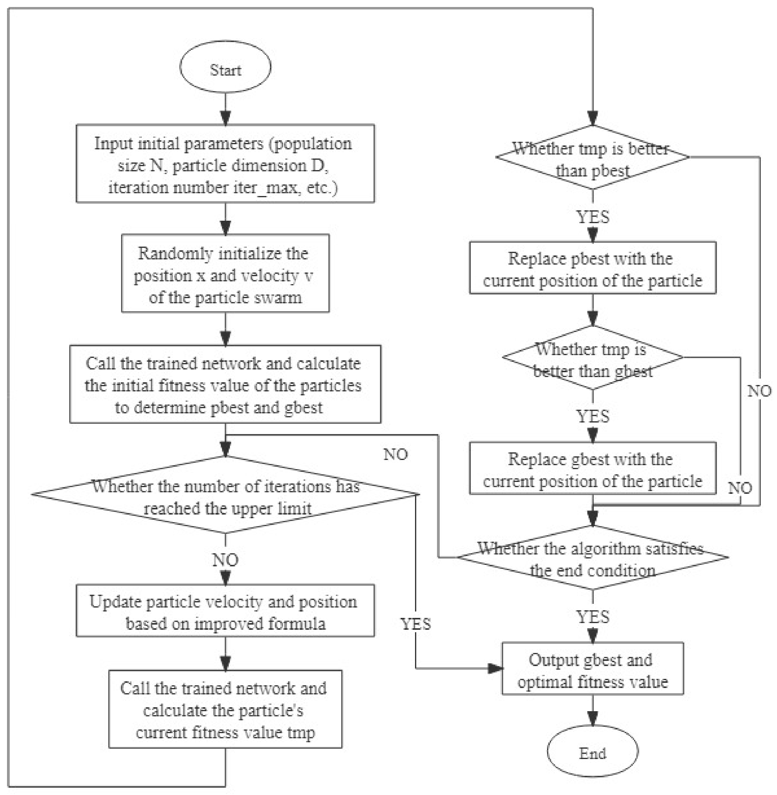
where $x_i^t$ is the solution of the current position of the particle; $x_i^{t+1}$ is the solution of the next random position of the particle; $v_i^{t+1}$ is the current velocity of the particle; $iter$ is the current number of iterations of the particle; $rand$ is a random number from zero to one; and C is a constant. In Formula (10), the range of random position of particles decreases with an increase in the number of iterations of particles, which is beneficial to improve the development capability of particles in the later stage. The optimization design steps are shown in Figure 3.

6. Experimental Results and Analysis

The experimental environment of this paper is as follows: In terms of hardware, the experiment relies on the laboratory’s own server; the experimental environment is the Ubuntu operating system, and the version number is 18.04. The server model is an Intel(R) Core(TM) I7-10700 CPU @ 2.90 GHz, with a total of 16 cores. In terms of software, the experimental data in this paper were obtained by programming in the Eclipse reservoir numerical simulation software. The optimization algorithm was written in the Python language; the development tool was PyCharm. The program was run in the Anaconda virtual environment; the Anaconda version number was 4.10, and the Python version number was 3.6.

6.1. Algorithm Basic Settings

In order to verify the effectiveness of the algorithm in this paper, the proposed CAPSO algorithm and SA-CAPSO algorithm are compared with the standard PSO algorithm, genetic algorithm (referred to as GA) and other algorithms in other literatures. The comparison algorithm uses the corresponding formula to replace the linear adaptation of the parameter w in the PSO, and the CAPSO and SA-CAPSO use the corresponding Formula (8) to replace the parameter w. To demonstrate the performance of the improved algorithm, we reduced the parameter value to optimize the solution process.The common parameters in all optimization algorithms are as follows: The number of populations N, is set to 20, the iteration is 100 times, and the dimension is five. The experiment uses the unimodal function and the multimodal function to test the above three algorithms, such as the five test functions shown in

Table 5. Five kinds of test functions for function extreme value optimization.

No.	Function Name	Test Function	Search Space	Optimal Solution
F1	Sphere	$f\left(x\right)={\sum }_{i=1}^n{x}_i^2$	[−100, 100]	0
F2	Schwefel 2.22	$f\left(x\right)={\sum }_{i=1}^n\left|x_i\right|+{\prod }_{i=1}^n\left|x_i\right|$	[−10, 10]	0
F3	Rosenbrock	$f\left(x\right)={\sum }_{i=1}^{n-1}[100{(x_{i+1}-x_i^2)}^2+{(x_i-1)}^2]$	[−30, 30]	0
F4	Step	$f\left(x\right)={\sum }_{i=1}^n{\left(\lfloor x_i+0.5\rfloor \right)}^2$	[−100, 100]	0
F5	Rastrigin	$f\left(x\right)={\sum }_{i=1}^n(x_i^2-10cos\left(2\pi x_i\right)+10)$	[−5.12, 5.12]	0

, and finds the extreme value of the five functions. In order to make the analysis more accurate, each algorithm runs 15 times independently in the experiment. To make the analysis more meaningful, three different statistical parameters, mean, minimum and variance are used to evaluate the performance of the algorithm.

6.2. Comparison and Analysis of Experimental Results of PSO, CAPSO and SA-CAPSO

The key parameter w in PSO adopts linear adaptation (Formula (7)), and CAPSO and SA-CAPSO adopt cosine adaptation (Formula (8)) to replace Formula (7) in PSO. We conducted sensitivity experiments and selected two representative functions, namely test functions F1 and F2, and displayed the experimental results. The experimental results are shown in

Table 6. The solution result of the test function F1.

Algorithm	Dimension	Minimum	Mean	Variance	Time/s
PSO	2	9.08 × ${10}^{-7}$	3.51 × ${10}^{-4}$	2.05 × ${10}^{-4}$	0.23
	5	1.35 × ${10}^{-4}$	1.56 × ${10}^{-4}$	1.80 × ${10}^{-4}$	0.36
	10	3.98 × ${10}^{-2}$	2.71 × ${10}^{-1}$	9.65 × ${10}^{-1}$	0.51
	30	1.65	6.99	6.35	1.12
CAPSO	2	2.12 × ${10}^{-7}$	9.14 × ${10}^{-5}$	2.95 × ${10}^{-5}$	0.25
	5	3.06 × ${10}^{-5}$	1.13 × ${10}^{-4}$	1.51 × ${10}^{-4}$	0.28
	10	3.18 × ${10}^{-2}$	9.77 × ${10}^{-2}$	1.90 × ${10}^{-1}$	0.53
	30	1.51	6.16	6.62	1.08
SA-CAPSO	2	9.83 × ${10}^{-8}$	8.04 × ${10}^{-5}$	4.30 × ${10}^{-5}$	0.20
	5	8.70 × ${10}^{-6}$	4.82 × ${10}^{-4}$	2.88 × ${10}^{-4}$	0.25
	10	1.10 × ${10}^{-2}$	7.75 × ${10}^{-2}$	1.51 × ${10}^{-2}$	0.50
	30	1.18	6.69	6.50	1.04

and

Table 7. The solution result of the test function F2.

Algorithm	Dimension	Minimum	Mean	Variance	Time/s
PSO	2	9.51 × ${10}^{-5}$	2.38 × ${10}^{-3}$	3.99 × ${10}^{-3}$	0.20
	5	6.00 × ${10}^{-3}$	5.60 × ${10}^{-2}$	5.60 × ${10}^{-2}$	0.27
	10	2.40 × ${10}^{-1}$	4.71 × ${10}^{-1}$	2.43 × ${10}^{-1}$	0.43
	30	2.08	2.84	2.75	1.86
CAPSO	2	8.91 × ${10}^{-6}$	8.42 × ${10}^{-4}$	6.32 × ${10}^{-4}$	0.11
	5	7.77 × ${10}^{-3}$	5.05 × ${10}^{-2}$	2.48 × ${10}^{-2}$	0.26
	10	2.00 × ${10}^{-1}$	3.97 × ${10}^{-1}$	2.34 × ${10}^{-1}$	0.27
	30	1.83	2.77	2.99	1.68
SA-CAPSO	2	7.50 × ${10}^{-5}$	9.62 × ${10}^{-4}$	3.64 × ${10}^{-3}$	0.24
	5	3.44 × ${10}^{-3}$	8.40 × ${10}^{-2}$	8.20 × ${10}^{-2}$	0.34
	10	1.82 × ${10}^{-1}$	6.59 × ${10}^{-1}$	6.94 × ${10}^{-1}$	1.02
	30	1.71	2.88	3.01	1.34

.

Table 6 and Table 7 shows the comparison of PSO, CAPSO and SA-CAPSO in 2, 5, 10 and 30 dimensions respectively. It can be seen from the optimal results, average results and variance in the table that CAPSO and SA-CAPSO are superior to PSO in obtaining minimum and mean, but the variance is not necessarily better than PSO. It can be seen from the table that the curve adaptation has obvious advantages in low dimensions; the higher the dimension, the less obvious the advantages, and the difference between them is not much. On the whole, there is no significant difference in variance results and do not affect the overall conclusion. CAPSO and SA-CAPSO show better convergence performance than PSO.

6.3. Comparison and Analysis of Experimental Results between CAPSO and SA-CAPSO and Other Algorithms

GDIWPSO, SAPSO, OscTri, S-PSO, and IPSO are from the cited references [16,17,18,19,20], respectively, and they are improved algorithms for linearly decreasing inertia weights based on PSO and combined with various formulas respectively. They are compared with GA, which, like PSO, was proposed to solve combinatorial optimization problems. The experimental results are shown in

Table 8. Test results of test function F1.

Algorithm	Minimum	Mean	Variance	Time/s
PSO	1.35 × ${10}^{-4}$	1.56 × ${10}^{-4}$	1.80 × ${10}^{-4}$	0.36
GDIWPSO	9.30 × ${10}^{-4}$	2.36 × ${10}^{-3}$	8.59 × ${10}^{-3}$	0.22
SAPSO	1.87 × ${10}^{-5}$	1.17 × ${10}^{-4}$	6.58 × ${10}^{-5}$	0.35
Osc Tri	2.53 × ${10}^{-5}$	2.36 × ${10}^{-4}$	6.00 × ${10}^{-5}$	0.46
S-PSO	8.66 × ${10}^{-4}$	1.49 × ${10}^{-3}$	6.24 × ${10}^{-3}$	0.38
IPSO	6.70e × ${10}^{-4}$	7.95 × ${10}^{-3}$	4.05 × ${10}^{-3}$	0.35
GA	3.80 × ${10}^{-4}$	2.38 × ${10}^{-3}$	1.21 × ${10}^{-3}$	1.25
CAPSO	3.06 × ${10}^{-5}$	1.13 × ${10}^{-4}$	1.51 × ${10}^{-4}$	0.28
SA-CAPSO	8.70 × ${10}^{-6}$	4.82 × ${10}^{-4}$	2.88 × ${10}^{-4}$	0.25

,

Table 9. Test results of test function F2.

Algorithm	Minimum	Mean	Variance	Time/s
PSO	6.00 × ${10}^{-3}$	5.60 × ${10}^{-2}$	3.91 × ${10}^{-2}$	0.27
GDIWPSO	9.22 × ${10}^{-3}$	3.63 × ${10}^{-2}$	9.43 × ${10}^{-3}$	0.22
SAPSO	5.99 × ${10}^{-3}$	4.94 × ${10}^{-3}$	7.47 × ${10}^{-2}$	0.50
Osc Tri	2.45 × ${10}^{-2}$	4.78 × ${10}^{-2}$	3.06 × ${10}^{-2}$	0.63
S-PSO	2.07 × ${10}^{-2}$	6.54 × ${10}^{-2}$	6.84 × ${10}^{-2}$	0.54
IPSO	4.96 × ${10}^{-3}$	6.16 × ${10}^{-2}$	2.69 × ${10}^{-2}$	0.24
GA	2.69 × ${10}^{-2}$	9.29 × ${10}^{-2}$	3.61 × ${10}^{-2}$	1.40
CAPSO	7.77 × ${10}^{-3}$	5.05 × ${10}^{-2}$	2.48 × ${10}^{-2}$	0.26
SA-CAPSO	3.44 × ${10}^{-3}$	8.40 × ${10}^{-2}$	8.20 × ${10}^{-2}$	0.34

,

Table 10. Test results of test function F3.

Algorithm	Minimum	Mean	Variance	Time/s
PSO	1.70 × ${10}^{-4}$	1.61 × ${10}^{-3}$	2.85 × ${10}^{-4}$	0.31
GDIWPSO	9.98 × ${10}^{-4}$	1.95 × ${10}^{-3}$	1.70 × ${10}^{-3}$	0.31
SAPSO	1.47 × ${10}^{-4}$	3.04 × ${10}^{-4}$	9.86 × ${10}^{-4}$	0.33
Osc Tri	9.90 × ${10}^{-5}$	4.54 × ${10}^{-4}$	1.13 × ${10}^{-4}$	0.39
S-PSO	4.93 × ${10}^{-5}$	1.39 × ${10}^{-4}$	1.88 × ${10}^{-4}$	0.27
IPSO	8.48 × ${10}^{-4}$	4.85 × ${10}^{-3}$	3.83 × ${10}^{-3}$	0.23
GA	5.08 × ${10}^{-3}$	1.59 × ${10}^{-2}$	4.06 × ${10}^{-4}$	1.23
CAPSO	5.92 × ${10}^{-5}$	2.78 × ${10}^{-4}$	6.14 × ${10}^{-4}$	0.27
SA-CAPSO	2.14 × ${10}^{-5}$	1.10 × ${10}^{-3}$	4.40 × ${10}^{-4}$	0.29

,

Table 11. Test results of test function F4.

Algorithm	Minimum	Mean	Variance	Time/s
PSO	0	6.50 × ${10}^{-4}$	8.76 × ${10}^{-4}$	0.22
GDIWPSO	0	1.20 × ${10}^{-3}$	0.94 × ${10}^{-3}$	0.24
SAPSO	0	0.94 × ${10}^{-3}$	0.87 × ${10}^{-4}$	0.21
Osc Tri	0	1.12 × ${10}^{-3}$	1.00 × ${10}^{-3}$	0.29
S-PSO	0	0.96 × ${10}^{-3}$	1.01 × ${10}^{-3}$	0.21
IPSO	0	0.65 × ${10}^{-3}$	0.76 × ${10}^{-3}$	0.26
GA	0	0.90 × ${10}^{-3}$	0.84 × ${10}^{-3}$	1.20
CAPSO	0	0.55 × ${10}^{-3}$	0.80 × ${10}^{-3}$	0.21
SA-CAPSO	0	0.48 × ${10}^{-3}$	0.70 × ${10}^{-3}$	0.18

and

Table 12. Test results of test function F5.

Algorithm	Minimum	Mean	Variance	Time/s
PSO	5.87 × ${10}^{-3}$	1.04 × ${10}^{-2}$	4.61 × ${10}^{-2}$	0.38
GDIWPSO	6.70 × ${10}^{-3}$	6.04 × ${10}^{-2}$	1.33 × ${10}^{-2}$	0.33
SAPSO	1.56 × ${10}^{-3}$	1.59 × ${10}^{-3}$	1.44 × ${10}^{-2}$	0.41
Osc Tri	7.10 × ${10}^{-4}$	2.03 × ${10}^{-3}$	1.54 × ${10}^{-3}$	0.49
S-PSO	2.35 × ${10}^{-3}$	7.11 × ${10}^{-3}$	4.00 × ${10}^{-3}$	0.40
IPSO	3.18 × ${10}^{-3}$	5.50 × ${10}^{-3}$	3.61 × ${10}^{-3}$	0.24
GA	4.64 × ${10}^{-3}$	4.92 × ${10}^{-3}$	1.36 × ${10}^{-2}$	1.29
CAPSO	9.01 × ${10}^{-4}$	1.63 × ${10}^{-3}$	4.53 × ${10}^{-3}$	0.21
SA-CAPSO	6.18 × ${10}^{-4}$	5.74 × ${10}^{-3}$	1.81 × ${10}^{-3}$	0.35

.

Table 8, Table 9, Table 10, Table 11 and Table 12 shows the comparison results of CAPSO, SA-CAPSO, PSO, GDIWPSO, SAPSO, OscTri, S-PSO, IPSO and GA under 5 dimensions. As can be seen from the results in the table, for the test functions F1–F3 and F5, SA-CAPSO is superior to other improved algorithms in obtaining the minimum value, has obvious advantages over other improved algorithms, and the solution accuracy is higher, indicating that the proposed algorithm has a good convergence effect. CAPSO may be slightly better or worse than other improved algorithms, but it performs better in average results and variance. For F4, the minimum value can converge to zero, the time of the method in this paper is slightly better, and the time to converge to the extreme value of the function is shorter. The comparison shows that CAPSO has good stability, and SA-CAPSO has higher convergence accuracy, which also reflects that the curve adaptation modification parameter w is better than the linear adaptation parameter in PSO.

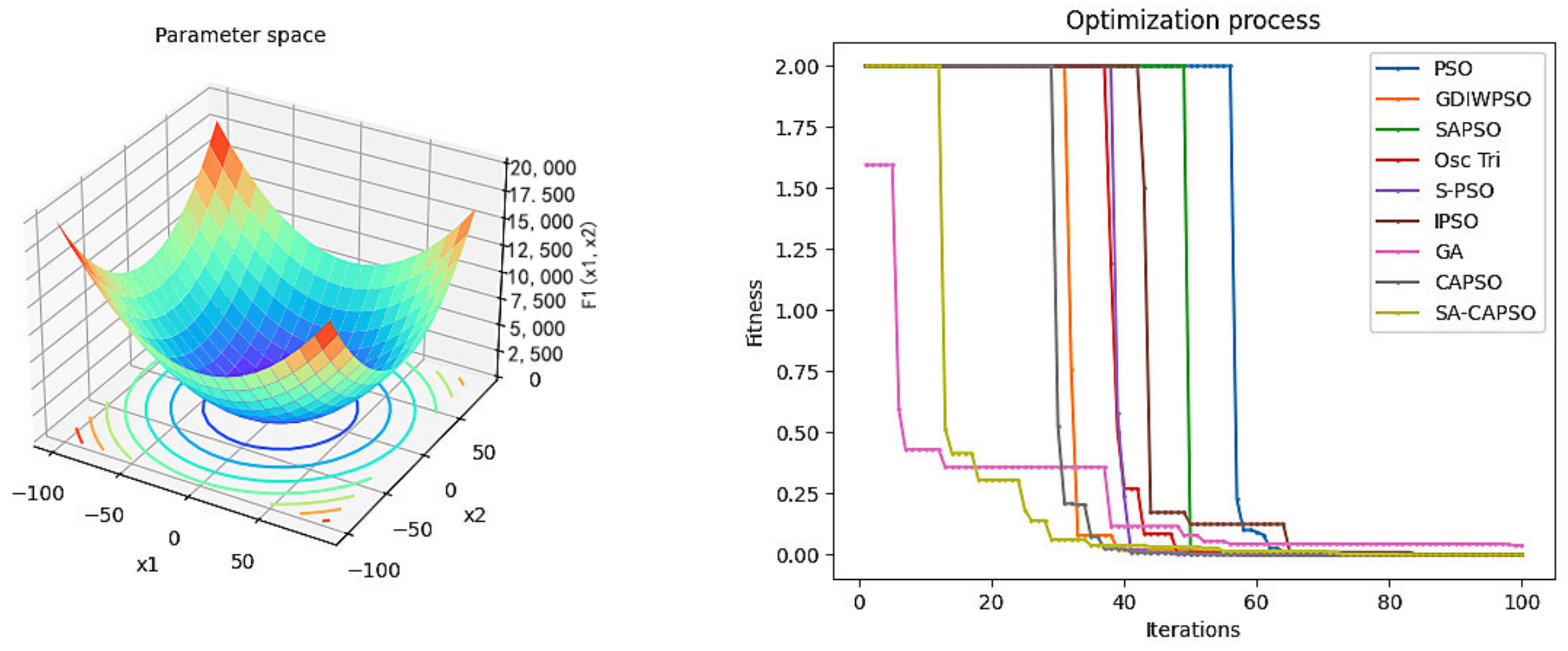
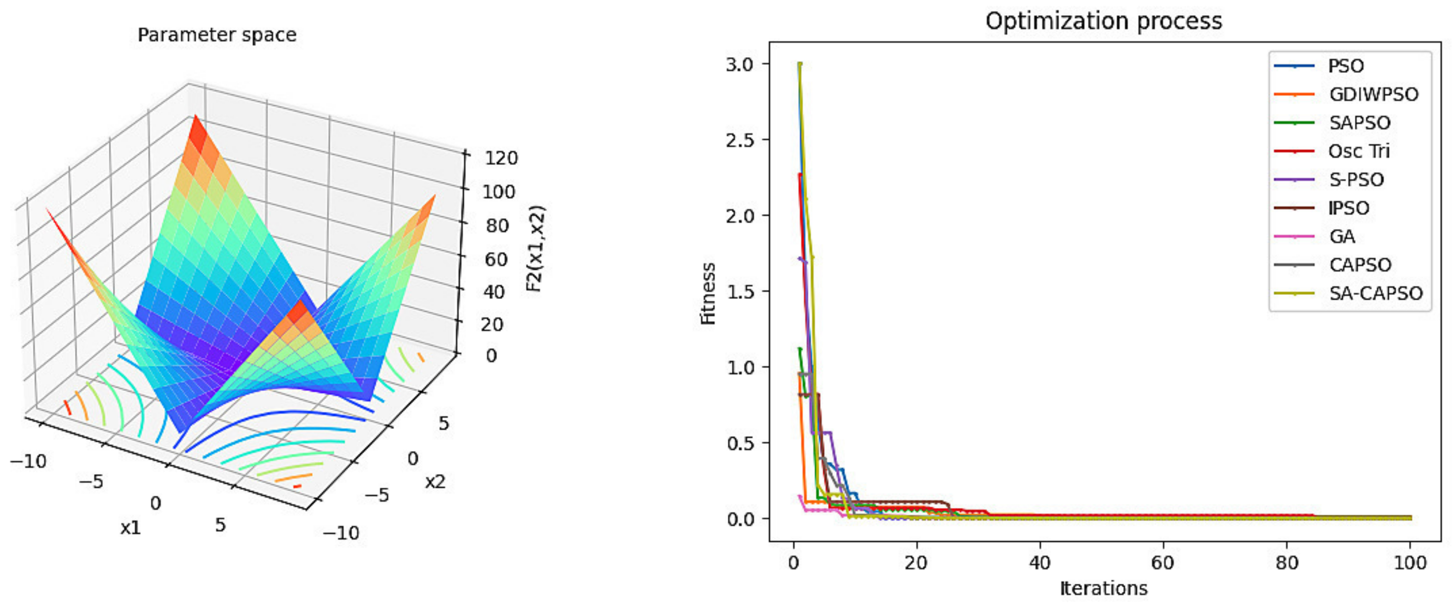
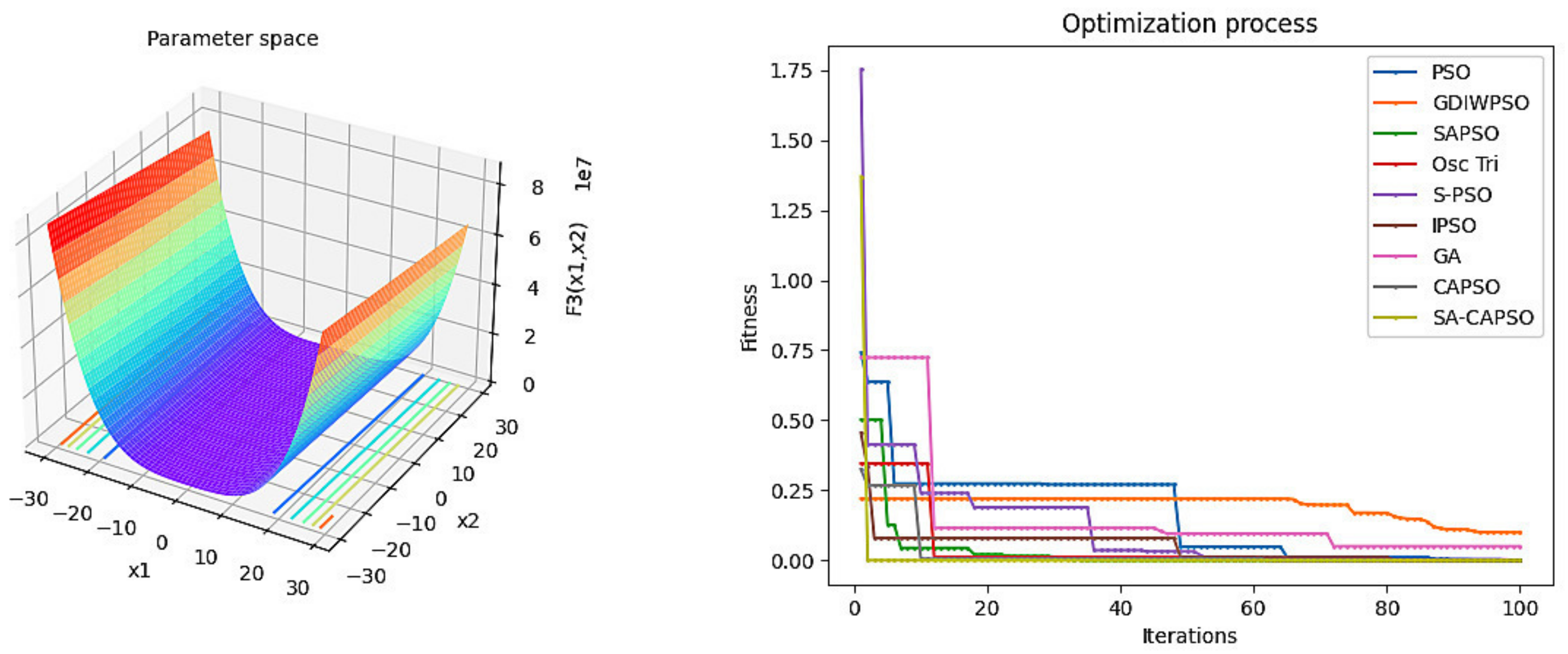
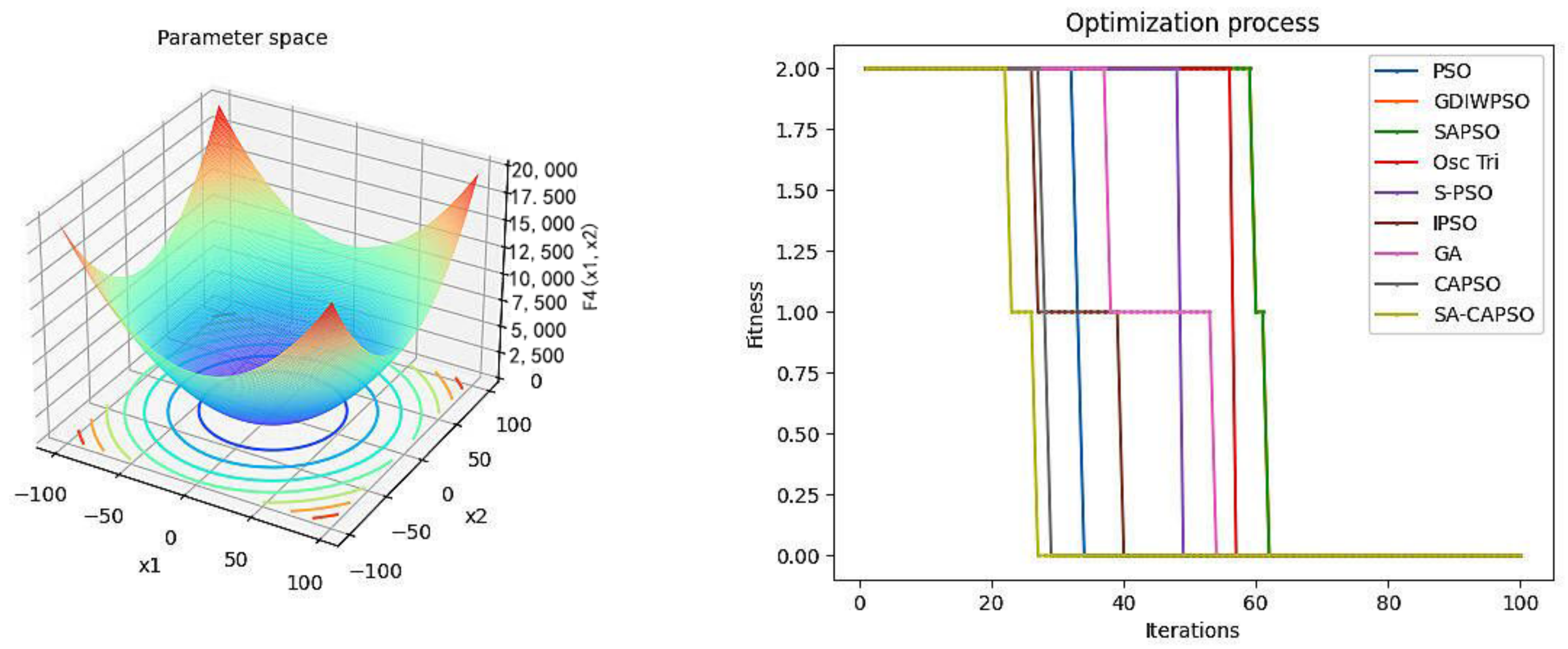
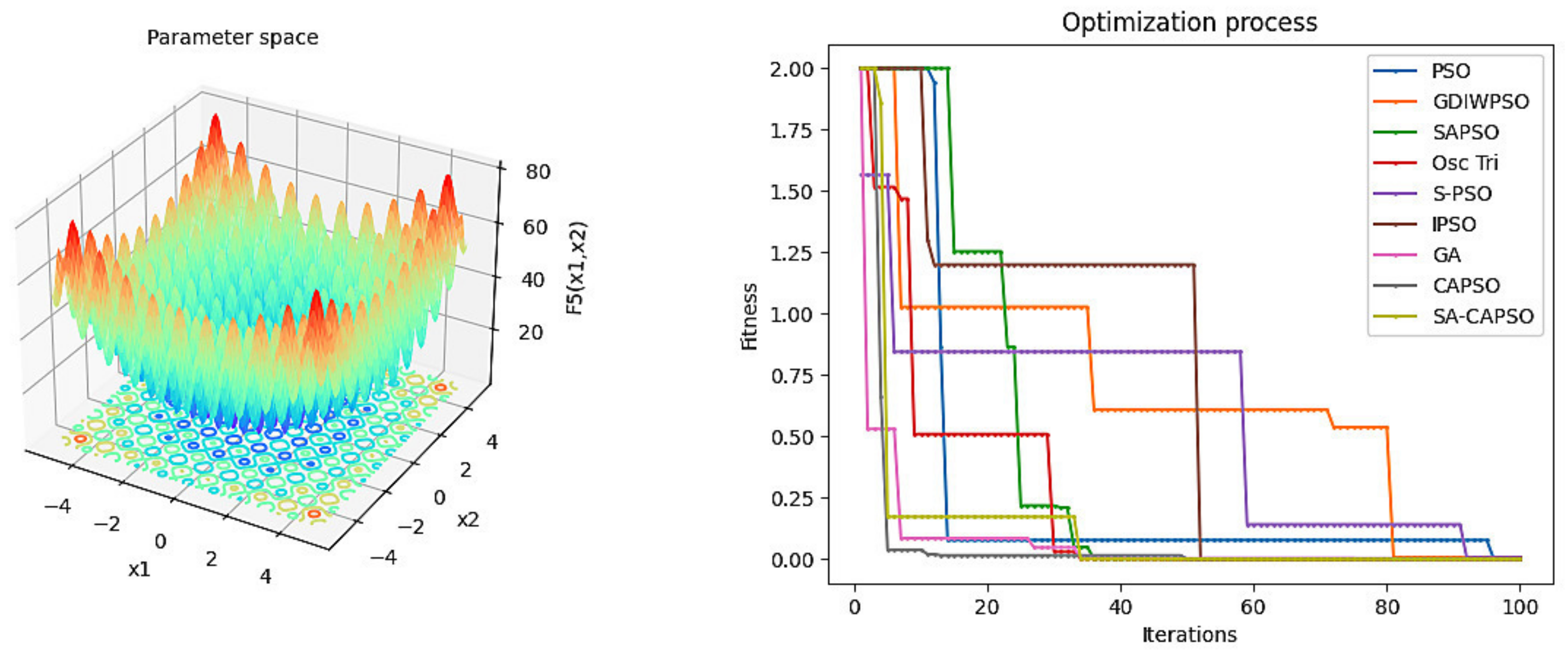
The update formula of the parameter w provided by the curve adaptation to replace the linear update has a better experimental effect, and can provide a good balance between exploration and development, preventing the algorithm from stagnant position during the optimization process. Finally, CAPSO, SA-CAPSO, PSO, GDIWPSO, SAPSO, OscTri, S-PSO, IPSO, and GA are compared in terms of optimization performance. The iteration curve of the optimal fitness value is shown in Figure 4, Figure 5, Figure 6, Figure 7 and Figure 8.

It can be seen from the iterative curve of function optimization in Figure 4, Figure 5, Figure 6, Figure 7 and Figure 8 that the overall convergence speed of the improved particle swarm optimization algorithm is faster and the accuracy of the solution can be improved. This is because the particle uses the simulated annealing algorithm to optimize the current particle position in each iteration process, and the range selection of the particle random solution in simulated annealing (Formula (10)) decreases with the increase of the number of particle iteration times, which greatly promotes the later development ability of the particle and improves the accuracy of the optimal solution of the particle. SA-CAPSO has higher convergence accuracy on the whole, which shows that the curve adaptation can well balance the transition of particles from exploration to development.

6.4. Nonparametric Statistical Test

In order to verify the significant difference between the SA-CAPSO algorithm proposed in this paper and other algorithms, a non-parametric estimation method-Wilcoxon rank sum test is used for statistical analysis. For each test function, the 15 times solution results of SA-CAPSO and the 15 times solution results of other algorithms are respectively tested for hypothesis. Among them: it is assumed that there is no significant difference between the mean values of the two algorithms at H0, and there is a significant difference between the mean values of the two algorithms at H1. Set the null hypothesis test significance level threshold $\alpha =0.05$. When the test result $p<0.05$, the null hypothesis is rejected, and the experimental result of the two algorithms is significantly different; when the test result $p>0.05$, the null hypothesis is accepted, then there is no significant difference in the experimental result of the two algorithms.

Table 13. Wilcoxon Rank Sum Test Results.

Test Functions	Indicators	F1	F2	F3	F4	F5
SA-CAPSO vs. PSO	P	6.9115 × ${10}^{-9}$	5.988 × ${10}^{-8}$	4.6785 × ${10}^{-13}$	0.000087	4.5405 × ${10}^{-7}$
	W	+	+	+	+	+
SA-CAPSO vs. GDIWPSO	P	0.104050	6.8691 × ${10}^{-8}$	4.7814 × ${10}^{-10}$	9.1015 × ${10}^{-10}$	0.000941
	W	=	+	+	+	+
SA-CAPSO vs. SAPSO	P	0.249648	2.1896 × ${10}^{-11}$	5.2079 × ${10}^{-8}$	2.3821 × ${10}^{-8}$	0.000778
	W	=	+	+	+	+
SA-CAPSO vs. Osc Tri	P	2.4114 × ${10}^{-13}$	1.6624 × ${10}^{-11}$	0.000041	6.8914 × ${10}^{-9}$	5.9952 × ${10}^{-14}$
	W	+	+	+	+	+
SA-CAPSO vs. S-PSO	P	0.000003	1.2895 × ${10}^{-11}$	7.8895 × ${10}^{-10}$	2.0854 × ${10}^{-7}$	4.4409 × ${10}^{-16}$
	W	+	+	+	+	+
SA-CAPSO vs. IPSO	P	4.6212 × ${10}^{-12}$	0.027877	0.056548	0.000006	0.000661
	W	+	+	=	+	+
SA-CAPSO vs. GA	P	0.004984	0.0 × ${10}^0$	0.000143	3.482 × ${10}^{-8}$	0.0 × ${10}^0$
	W	+	+	+	+	+
SA-CAPSO vs. CAPSO	P	0.027984	3.2051 × ${10}^{-9}$	0.000002	0.000474	0.0 × ${10}^0$
	W	+	+	+	+	+

shows the test results of the test function F1–F5 with dimension 5. Among them, “W” is the judgment result of the test of significance; Combined with Table 6, Table 7, Table 8, Table 9, Table 10, Table 11 and Table 12, “+” indicates that SA-CAPSO has higher solving accuracy and has significant difference compared with other algorithms. “=” indicates that there is no significant difference in the solution accuracy between the SA-CAPSO algorithm and other algorithms. From the test results, most of the test p value is less than 0.05 and “W” is “+”, rejecting the null hypothesis. In addition, statistical tests were carried out on the results of F1–F5 calculation under the dimensions of 10 and 30, and the overwhelming majority of results rejected the null hypothesis. Therefore, on the whole, there is a significant difference between the calculation results of SA-CAPSO and other algorithms, and SA-CAPSO is significantly better.

6.5. Test Results of Injection-Production Parameters

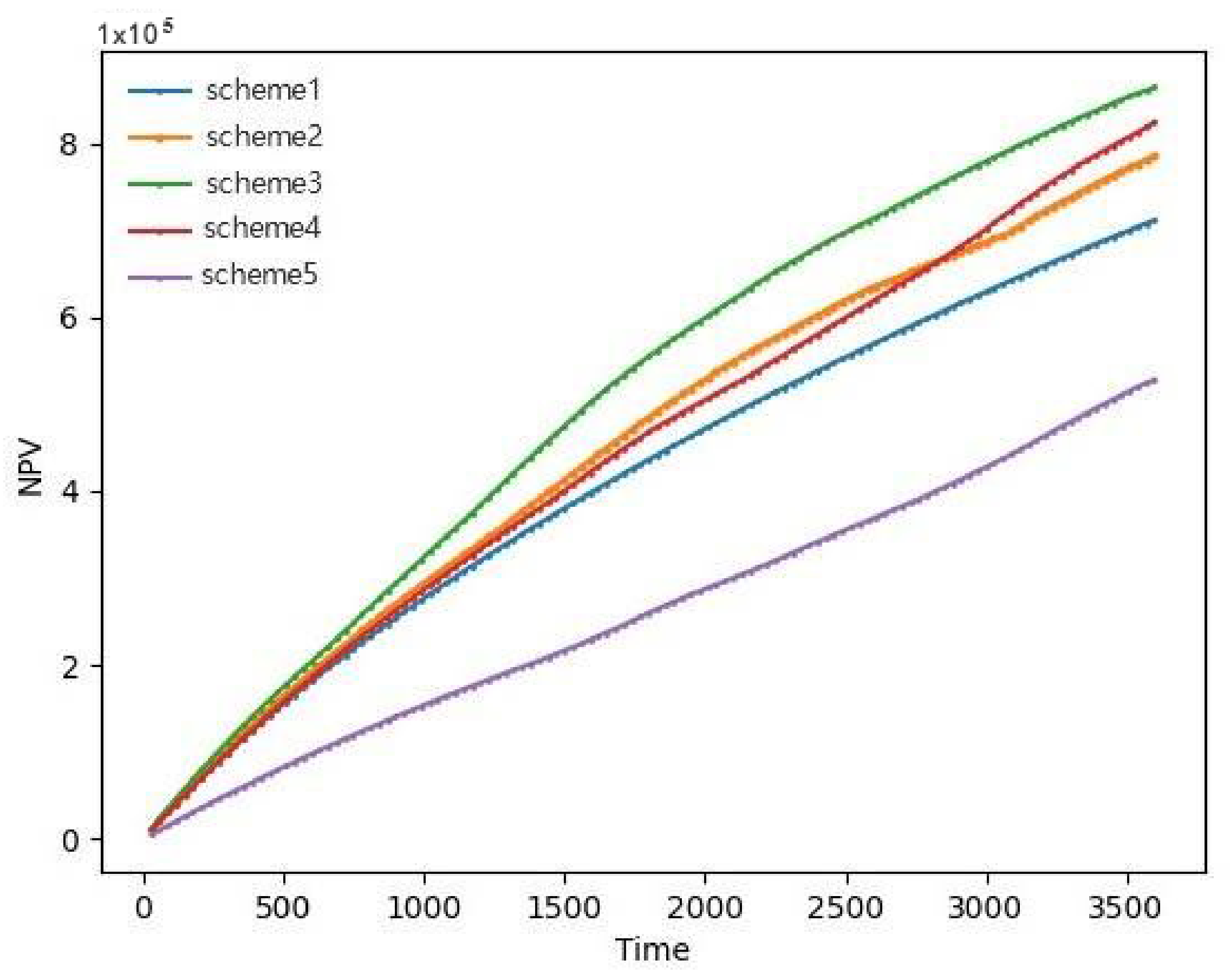
As shown in Figure 9 below, the five lines of five colors in the graph represent different injection-production schemes, the abscissa represents the time, which is the number of production days, and the ordinate represents the net present value. The bigger the net present value the better, so curve three is the best and curve five is the worst. The net present value represented by curve three is twice that of curve five, and the ordinate is ten thousand levels. Therefore, the difference in the net present value between different injection-production schemes is large, and the size of the NPV is greatly affected by injection-production parameters, which are sufficient to reflect the necessity of parameter optimization. Therefore, combined with practical applications, the injection-production parameters are optimized with the goal of increasing the net present value, which can improve the production efficiency and control the costs in oil field production.

According to the algorithm, the optimization program of a reservoir injection-production scheme is compiled in Python. The relevant parameters of the algorithm are as follows: Different from the multimodal function, it is easy to fall into the local optimal solution. The problem in this paper is relatively simple, so the particle population size N, is taken as 20; the particle dimension D, needs to be analyzed for specific problems, and it is consistent with the data dimension. Since the data have 41 dimensions, D should also be 41; in order to show the degree of improvement of the algorithm, this paper chooses a smaller number of iterations, and iter_max takes 50; because the training data are normalized, the particle position range is set at [0, 1]. This paper takes the optimization of the injection-production scheme of a gas injection reservoir in the Tarim oil field as an example for the trial calculation, and takes the net present value as the objective function to be optimized in addition to the production and injection regimes of all wells in each well pattern as the variables to be optimized. The improved particle swarm optimization algorithm is used to find the injection-production parameters corresponding to the maximum economic benefit.

Assuming that the reservoir area needs continuous gas injection and water injection, the standard PSO algorithm, CAPSO algorithm and SA-CAPSO algorithm are used to optimize the established reservoir injection-production scheme optimization model. A comparison of the results of different optimization schemes obtained according to the standard PSO algorithm, CAPSO algorithm and SA-CAPSO algorithm is shown in Figure 10.

It can be seen from Figure 10 that, after three different optimization methods are used for continuous gas injection and water injection, the net present values are 1.555 × 10⁷, 1.605 × 10⁷ and 1.606 × 10⁷, respectively. Compared with the results of the standard PSO optimization method, the SA-CAPSO optimization method increases the net present value by 3.28%.

It can be seen from the example of an optimization method of an oil reservoir injection-production scheme based on the particle swarm optimization algorithm of curve adaptation and simulated annealing, after continuous gas injection and water injection, that the net present value has increased to a certain extent, and it has the ability to jump out of the local optimum. By comparison, it is shown that this method can effectively improve the economic benefits of an oil field by determining an injection-production optimization scheme.

7. Conclusions

Aiming at the problem that particle swarm optimization is easy to fall into a local optimum, a particle swarm optimization algorithm based on curve adaptation (CAPSO) and a particle swarm optimization algorithm based on curve adaptation and simulated annealing (SA-CAPSO) were proposed, and the application strategy of the improved algorithm in the optimization of injection-production parameters was studied. Taking the maximum net present value as the goal, and the gas injection rate, water injection rate and flowing bottom hole pressure as constraint conditions, a mathematical model for optimizing the reservoir injection-production scheme was established. The improved algorithm was used to solve the model, and the global optimal solution of the net present value within a certain range was obtained. By comparison, it shows that the improved method is more reasonable and effective than the standard method.In addition, the method designed in this paper has certain generality. The application scenarios of the algorithm are not only the optimization of injection-production parameters, but also the optimization of other data, such as various single-parameter and multiparameter optimization problems and the problem of selecting the best parameters in other application scenarios.

References

- Zhang, Y.; Di, Y.; Shi, Y.; Hu, J. Cyclic CH4 Injection for Enhanced Oil Recovery in the Eagle Ford Shale Reservoirs. Energies 2018, 11, 3094. [Google Scholar] [CrossRef] [Green Version]
- Ni, H. Research on Steam Flooding Development Effectiveness Prediction and Parameter Optimization Method Based on Intelligent Computation. Ph.D. Thesis, Northeast Petroleum University, Heilongjiang, China, 31 May 2016. [Google Scholar]
- Tang, H.; He, J.; Rong, Y. Study on water drive law and characteristics of remaining oil distribution of typical fault-karst in fault-karst reservoirs, Tahe Oilfield. Pet. Geol. Recovery Effic. 2018, 25, 95–100. [Google Scholar]
- Yao, C.; Shao, Y.; Yang, J. Numerical Investigation on the Influence of Areal Flow on EGS Thermal Exploitation Based on the 3-D T-H Single Fracture Model. Energies 2018, 11, 3026. [Google Scholar] [CrossRef] [Green Version]
- Fang, N.; Zhang, Z.; Cheng, M. Injection-production parameter optimization study of cyclic water injection at different development levels of fractures. Spec. Oil Gas Reserv. 2019, 26, 131–135. [Google Scholar]
- Song, Y.; Xu, Y.; Cheng, X. Using a Genetic Algorithm to Achieve Optimal Matching between PMEP and Diameter of Intake and Exhaust Throat of a High-Boost-Ratio Engine. Energies 2022, 15, 1607. [Google Scholar] [CrossRef]
- Eisenmann, A.; Streubel, T.; Rudion, K. Power Quality Mitigation via Smart Demand-Side Management Based on a Genetic Algorithm. Energies 2022, 15, 1492. [Google Scholar] [CrossRef]
- He, Y.; Liu, J.; Yang, R. Survey on artificial bee colony algorithm. Appl. Res. Comput. 2018, 35, 1281–1286. [Google Scholar]
- Xiao, Y.; Wang, Y.; Sun, Y. Reactive Power Optimal Control of a Wind Farm for Minimizing Collector System Losses. Energies 2018, 11, 3177. [Google Scholar] [CrossRef] [Green Version]
- Zhang, X.; Yang, S.; Zhang, Z. Optimization of injection-production parameters for CO2/N2 composite gas huff and puff in fault-block reservoirs considering starting pressure gradient. Sci. Technol. Eng. 2021, 21, 14127–14132. [Google Scholar]
- Wang, W.; Shi, M.; Zhuang, X. Joint optimization method of well location and injection-production parameters based on machine learning. J. Shenzhen Univ. Sci. Eng. 2022, 39, 126–133. [Google Scholar]
- Wu, J.; Li, P.; Sun, Y. Neural network-based prediction of remaining oil distribution and optimization of injection-production parameters. Pet. Geol. Recovery Effic. 2020, 27, 85–93. [Google Scholar]
- Yu, H.; Hou, J.; Du, Q. Study on recovery of heavy oil reservoir and their contribution degree by oil displacing agent and viscosity reducing agent flooding. In Proceedings of the 2018 International Field Exploration and Development Conference, Xi’an, China, 18–20 September 2018. [Google Scholar]
- Zhang, F. Optimization method of injection-production parameters for polymer/surfactant binary flooding. J. China Univ. Pet. (Ed. Nat. Sci.) 2018, 42, 98–104. [Google Scholar]
- Charles, K.; Urasaki, N.; Senjyu, T.; Elsayed Lotfy, M.; Liu, L. Robust Load Frequency Control Schemes in Power System Using Optimized PID and Model Predictive Controllers. Energies 2018, 11, 3070. [Google Scholar] [CrossRef] [Green Version]
- Zhang, X.; Wang, P.; Xing, J. Particle swarm optimization algorithms with decreasing inertia weight based on Gaussian function. Appl. Res. Comput. 2012, 29, 3710–3712, 3724. [Google Scholar]
- Huang, Y.; Lu, H.; Xu, K. S-shaped Function Based Adaptive Particle Swarm Optimization Algorithm. Comput. Sci. 2019, 46, 245–250. [Google Scholar]
- Kordestani, J.K.; Rezvanian, A.; Meybodi, M.R. An efficient oscillating inertia weight of particle swarm optimisation for tracking optima in dynamic environments. J. Exp. Theor. Artif. Intell. 2016, 28, 137–149. [Google Scholar] [CrossRef]
- De, G.; Gao, W. Forecasting China’s Natural Gas Consumption Based on AdaBoost-Particle Swarm Optimization-Extreme Learning Machine Integrated Learning Method. Energies 2018, 11, 2938. [Google Scholar] [CrossRef] [Green Version]
- Li, J.; Gong, Y.; Zhao, S. Improvement of Particle Swarm Optimization Algorithm and Numerical Simulation. J. Jilin Univ. (Sci. Ed.) 2017, 55, 322–332. [Google Scholar]
- Kennedy, J.; Eberhart, R. Particle swarm optimization. In Proceeding of the ICNN’95-IEEE International Conference on Neural Networks, Perth, Australia, 27 November–1 December 1995. [Google Scholar]
- He, H.; Lu, Z.; Guo, X. Optimized Control Strategy for Photovoltaic Hydrogen Generation System with Particle Swarm Algorithm. Energies 2022, 15, 1472. [Google Scholar] [CrossRef]
- Dong, Y.; Zhang, Y.; Liu, F. Reservoir Production Prediction Model Based on a Stacked LSTM Network and Transfer Learning. ACS Omega 2021, 6, 34700–34711. [Google Scholar] [CrossRef]
- Li, Y.; Gu, L. Grasshopper optimization algorithm based on curve adaptive and simulated annealing. Appl. Res. Comput. 2018, 36, 3637–3643. [Google Scholar]
- Qu, J.; Xu, Q.; Sun, K. Optimization of Indoor Luminaire Layout for General Lighting Scheme Using Improved Particle Swarm Optimization. Energies 2022, 15, 1482. [Google Scholar] [CrossRef]
- Yan, Q.; Ma, R.; Ma, Y. Adaptative simulated annealing particle swarm optimization algorithm. J. Xidian Univ. 2021, 48, 120–127. [Google Scholar]
- Metropolis, N.; Rosenbluth, A.; Rosenbluth, M. NEquation of state calculations by fast computing machines. J. Chem. Phys. 1953, 21, 1087–1092. [Google Scholar] [CrossRef] [Green Version]
- Fu, W.; Ling, C. Brownian motion based simulated annealing algorithm. Chin. J. Comput. 2014, 37, 1301–1308. [Google Scholar]
- Wang, L.; Xu, R.; Jin, X. Comprehensive Evaluation and Comparison of Nonlinear Inversion About Simulated Annealing, Genetic Algorithm And Neural Network Algorithm. Geomat. Inf. Sci. Wuhan Univ. 2021. [Google Scholar] [CrossRef]
- Guo, M.; Wang, Y.; Liu, Y. Research on Q-learning algorithm based on Metropolis criterion. J. Comput. Res. Dev. 2002, 39, 684–688. [Google Scholar]
Figure 1.
Schematic diagram of particle movement.
Figure 2.
Variation curve of parameter w with the number of iterations.
Figure 3.
Optimization flow of SA-CAPSO algorithm.
Figure 4.
Two-dimensional function image and iterative curve of function F1.
Figure 5.
Two-dimensional function image and iterative curve of function F2.
Figure 6.
Two-dimensional function image and iterative curve of function F3.
Figure 7.
Two-dimensional function image and iterative curve of function F4.
Figure 8.
Two-dimensional function image and iterative curve of function F5.
Figure 9.
Changes in the NPV under different injection-production parameters.
Figure 10.
Changes of the NPV under different injection-production parameters.