
Large Eddy Simulations of a Low-Swirl Gaseous Partially Premixed Lifted Flame in Presence of Wall Heat Losses †


Department of Industrial Engineering, University of Florence, 50139 Florence, Italy
*
Author to whom correspondence should be addressed.
†
This paper is an extended version of our poster presented at the 10th European Combustion Meeting, Naples, Italy, 14–15 April 2021.
Energies 2022, 15(3), 788; https://doi.org/10.3390/en15030788
Submission received: 7 December 2021
/
Revised: 12 January 2022
/
Accepted: 18 January 2022
/
Published: 21 January 2022
(This article belongs to the Special Issue Advances in Heat Transfer and Combustion in Turbomachinery)
Abstract
:The use of lifted flames presents some very promising advantages in terms of pollutant emissions and flame stability. The focus here is on a specific low-swirl injection system operated with methane and derived from an air-blast atomizer for aero-engine applications, which is responsible for flame lift-off. The key feature of this concept is the interaction between the swirling jet and the confinement walls, leading to a strong outer recirculation zone and thus to an upstream transport of combustion products from the main reaction region to the flame base. Here, the representation of the physics involved is challenging, since finite-rate effects govern the lift-off occurrence, and only a few numerical studies have been carried out on this test case so far. The aim of the present work is therefore to understand the limits of some state-of-the-art combustion models within the context of LES. Considering this context, two different strategies are adopted: the Flamelet-Generated Manifold (FGM) approach and the Thickened Flame (TF) model. A modified version of the FGM model including stretch and heat loss effects is also applied as an improvement of the standard model. Numerical results are compared with the available experimental data in terms of temperature and chemical species concentration maps, showing that the TF model can better reproduce the lift-off than the FGM approach.
1. Introduction
Recently, research in the gas turbine (GT) field has focused on new combustion systems that are able to guarantee both low pollutant emission and safe operability among all the possible operating conditions. The first objective could be reached thanks to lean burn concepts, which in turn pose new challenges in terms of flame stability, flashback occurrence and Lean Blow-Off (LBO) limits. Indeed, in many current applications, these issues are faced by employing a partially premixed system, thus limiting the benefits of the concept in terms of nitrogen oxides () emissions. A possible improvement is represented by the use of lifted flames, characterized by a main reaction zone considerably detached from the nozzle outlet section by a distance often called the Lift-Off Height (LOH) in the literature. This flame has shown some advantages, above all the improvement of air–fuel mixing before the the flame front is reached with respect to the standard partially premixed burner concept. This allows one to safely operate with a lean equivalence ratio without using pilot injectors. At the same time, the flashback risk is avoided since air-fuel mixing occurs directly in the combustion chamber.
Such flames have been widely studied in the scientific literature in both academic test cases and industrial applications [1]. In the second case, the most diffused configuration is represented by jet flames, where pure fuel is injected in the combustion chamber [2,3]. Regarding the GT application field, two different concepts have been proposed, respectively, by Cheng [4] and Zarzalis [5], both employing low-swirl injectors. The latter one is particularly interesting since it is similar to a usual aero-engine nozzle, but with better performance in terms of reduction [5,6]. It has also demonstrated improved stability in terms of LBO occurrence [7,8], thus possibly allowing it to operate with even leaner equivalence ratios.
Although many experimental and numerical investigations have been performed on lifted flames in recent years, a complete understanding of the flame-stabilization mechanism is still missing. A possible explanation for this lack of knowledge can be found considering that many physical phenomena contribute to flame stabilization, and it is generally not possible to observe a unique mechanism acting alone [1,9]. Indeed, previous works on this topic have recognized the importance of the physics occurring in the lift-off region, as the zone where many effects occur in terms of the turbulence–chemistry interaction, thus affecting the final position of the flame base. Here, the turbulent flow-field could promote air–fuel mixing, as well as entrainment of the recirculating hot combustion products, which in turn control the ignition of the fresh mixture. Moreover, the occurrence of local quenching [1] and reduction of the global reactivity is not excluded. In this sense, a numerical approach could help to provide a complete view of the whole combustion process while at the same time avoiding affecting the flame with intrusive experimental techniques.
Considering the low-swirl burner investigated by Zarzalis and co-workers, as far as the authors are aware, very few numerical works have been carried out on this nozzle concept, which include a first study by Kern et al. [10] and a more recent one by Sedlmaier [11]. In both cases, the numerical simulations have shown an incorrect prediction of the reaction zone position, leading sometimes to the flame reattachment. This fact shows the challenges related to the numerical modeling of these flames. The aim of the present work is therefore to understand the limitations of two of the most popular turbulent combustion models within Large Eddy Simulations (LES) applied in the GT field: the Flamelet-Generated Manifold (FGM) and the Thickened Flame (TF) model. Indeed, a preliminary discussion of such comparison is available in [12].
This work follows a previous investigation carried out by the authors on the same injector concept, where the FGM approach and a modified version of such model including the stretch and heat loss effects were applied [13]. The outcomes showed that, although the lift-off occurrence was reproduced, the LOH was largely underestimated. In addition, the reaction zone shape and axial extension were not representative of the experimental measurements. However, improvement of the flame reproduction was obtained with the modified FGM due to the introduction of local quenching phenomena effects. The present work aims to further assess these two approaches considering the concentration of chemical species, which are available from the experimental campaign. On the other hand, the impact of the a priori assumptions on the combustion regime (i.e., the flamelet regime) and of the chemistry tabulation could be compared with a different combustion model, where no assumptions are made. To this aim, the TF model is employed as a well-established approach where the direct resolution of the flame front is accomplished.
2. Experimental Test Rig
The test rig considered here employs a confined low-swirl lifted flame investigated by Fokaides et al. at the Engler-Bunte Institut of the Karlsruhe Institute of Technology (KIT–EBI) [5,7]. The key feature of this burner is a radial double-swirl nozzle [14] with an overall theoretical swirl number below 0.4, where this number is defined as:
where is the angular momentum flux, is the inner radius of the prefilmer lip at the smallest section, and is the axial momentum flux. The injector is derived from an air-blast atomizer [14] and is constituted of a primary swirler with = 0.76 and a secondary swirler with a set of fully radial channels ( 0.0). This configuration leads to a particular flow-field where the Inner Recirculation Zone (IRZ) is weak and relatively small since it remains embedded within the high-velocity streams related to the secondary swirler. Conversely, a large Outer Recirculation Zone (ORZ) is present thanks to the interaction between the swirling jet of the nozzle and the confinement walls. This has a non-negligible extension in the axial direction, allowing combustion products to be transported from the reaction zone to the flame base.
During the experimental campaign, two different facilities were employed, respectively, for atmospheric pressure conditions and elevated pressure combustion: here, only the former was considered. The test rig provided a cylindrical combustion chamber where both gaseous and liquid fuel can be employed. The diameter was four times the throat diameter of the nozzle diffuser , and the outlet section was placed at a distance with equal to four and half times from the chamber bottom. Moreover, the outlet section geometry was designed to avoid back-flow recirculation. The main section consisted of a water-cooled ceramic segment, while different additional segments can be employed allowing for specific measurement techniques. Flow-field measurements were carried out by applying the Laser Doppler Anemometry (LDA) technique, thanks to two aligned silica-glasses for the optical access, for both isothermal and reactive conditions. Again concerning the reactive conditions, local species concentration in the combustion chamber was evaluated using gas sampling with a suction probe and then analyzed with conventional gas analyses based on molecular excitation process. In this fashion, spatial maps of chemical species such as carbon monoxide (CO), carbon dioxide (CO), and methane (CH) are available for the lift-off region and the main reaction zone. Finally, temperature measurements were obtained thanks to S type compensated micro thermocouple probes corrected for radiative heat losses. A sketch of the test rig comprehensive of the measurements segments can be found in [5].
The operating point studied in the present work employed methane as fuel. A summary of the test conditions is reported in Table 1. A lean global equivalence ratio equal to 0.65 is employed to investigate the flame stabilization and capability. Furthermore, the flame has been observed to also be stable for leaner operating conditions, when air pre-heating is increased [5,7,11].
3. Flame Characteristics
The main feature of this type of flame is clearly lift-off occurrence, which places the flame stably downstream the nozzle exit. The region before the main reaction zone has paramount importance, since here the mixing between fuel and oxidizer is accomplished and a quasi-premixed combustion regime is reached [5] without the requirement for dedicated devices (e.g., premixing plenums). This kind of stabilization, as mentioned, is allowed by the upstream transport of hot vitiated gas from the principal reaction zones due to the ORZ: its relevance is such that the flame cannot be ignited without confinement walls [5]. Furthermore, the temperature of recirculating gas has a primary role in the ignition of incoming fresh mixture [7]. This fact also highlights the importance of the heat losses through confinement walls, which could cool the transported products and thus postpone the mixture ignition and elevate the lift-off height. The heat transfer from hot gas surrounding the jet and its core are related to the entrainment of hot gas pockets due to Kelvin–Helmholtz instabilities at the jet surface. This aspect has a large impact also on the combustion modeling, as shown in [13], and it will later be discussed in detail.
Other parameters that affect the LOH magnitude are related to the operating conditions [8,15] and some geometry features [6], such as the ratio between the nozzle outlet section diameter and the combustion chamber diameter (i.e., the confinement ratio). All these aspects contribute again to the fresh mixture pre-heating before the flame front and influence the turbulence levels in the lift-off region. In conclusion, the lift-off region is dominated by several physical effects, which in turn directly control the turbulent flame speed and ultimately the stabilization position for the flame. Finally, the flame topology shows an arrow-like shape, where the flame base is anchored on the outer shear layer of the swirling jet: such morphology is very similar to a tribranchial flame structure, even if proof of its existence is not supported by the local equivalence ratio and flow-field [5].
4. Combustion Modeling
4.1. FGM Model
The use of laminar flame libraries for turbulent combustion modeling through the use of Probability Density Functions (PDF) for the description of the turbulence effects was originally proposed by Bradley et al. [16,17]. The underlying idea is that combustion occurs in a flamelet regime where the flame front is only distorted by the turbulence, and it could be described locally by laminar one-dimensional flames.
Considering the partially premixed combustion framework, one of the most popular approaches is the Flamelet-Generated Manifold model [18], where a number of these flamelets are solved in pre-processing and the associated thermochemical trajectories are parametrized in a look-up table as a function of two variables, the mixture fraction z (as defined by Bilger [19]) and the progress variable c. In this work, the progress variable is defined as , where is the un-normalized progress variable and is its value at equilibrium. The turbulence–chemistry interaction is taken into account by pre-integrating the look-up table using presumed -shaped PDF (or ): the reactive process is described using the mean values of the scalar and their respective variances (i.e., , , , ).
During the CFD simulations, three dedicated transport equations are employed to evaluate these scalars concerning the mean quantities and the variance of the progress variable, whereas the mixture fraction variance is closed through an algebraic formulation: for the sake of brevity, the equations are not reported here, and the interested reader is referred to [20]. Finally, the look-up table is queried for retrieving information about the chemical species and the flame. In this work, the progress variable source term is modeled with a Finite Rate approach, which is the source term is taken directly from the flamelets library: this term governs the flame propagation, and its correct estimation is of primary importance. The GRI3.0 detailed mechanism [21] with 325 reactions and 53 species is used for the table computation by freely propagating premixed flamelets, and it is discretized with points in terms of, respectively, z and c. The 1D laminar flame simulations adopts as an inlet temperature for the mixture, where is assumed equal to 300 K and is set accordingly to the test conditions of Table 1, as well as for the operating pressure.
One of the main advantages of this approach is that detailed chemistry can be used during the pre-processing operations, thus allowing for information for a large number of chemical species to be available with a low computational effort at run time. However, the critical aspect consists of how this table is computed, and for this reason, different strategies have been proposed [22,23], based on different 1D structures. Improving the accuracy of such a model implies employing a look-up table with many different parameters, which could reduce the advantage of a low computational effort. It should be noticed that this approach is similar to the one employed in previous numerical works [10,11], but the chemistry here was reduced a priori to one reaction pathway, and only 6 species were involved: according to the authors, this fact does not impact the final results unless the combustion occurs in lean conditions.
4.2. FGM-EXT Model
To improve the FGM model model’s predictions, the scientific community has put much effort into the inclusion of quenching effects due to local aerodynamic stretch and heat losses on the flame front. Several strategies have therefore been carried out, but basically, they could be divided into two different subgroups, as summarized in [24]: the direct inclusion of stretch and heat loss in the manifold by increasing its dimension, and the correction of the FGM reaction source term with a scaling factor while the original manifold is kept.
The first approach is theoretically the most correct, but it leads to complex strategies for using the look-up table and usually a very large manifold. These aspects could impact the computational effort required at runtime, and its implementation in the CFD solver is also not trivial. To limit the number of variables required for tabulation, sometimes only the heat loss is considered without the stretch [25,26,27] or the assumption of a fully premixed regime is made (i.e., avoiding the need for and ) [24].
The second approach is simpler since only the reaction rate takes into account the effects of stretch and heat loss: the scaling is obtained through the ratio of the laminar flame speed from unstrained and adiabatic flamelets to the ones from non-adiabatic strained flames. In addition, the use of such a scaling factor requires some assumptions depending on how it is defined, which rarely can be generalized for all the possible operating conditions. Overall, this strategy is quite straightforward to implement but at the expense of a less robust theoretical background. A further discussion of the advantages and drawbacks of these two approaches is outside the scope in the present work, while a very detailed description of these strategies with the related references is present in [24].
Since the second approach is used here, the focus is on the previous works that followed such strategy. In particular, the idea of applying a scaling factor to the reaction rate model was originally proposed by Tay-Wo-Chong et al. [28,29], along with the Turbulent Flame Closure model by Zimont [30], and a model developed at KIT–EBI [31]. Most recently, the same approach was applied in the work of Kutkan et al. [32] for flames employing blended methane–hydrogen mixtures. A further development was carried out by Klarmann et al. concerning the Finite Rate closure for the progress variable equation [33,34,35]. Both of these approaches were developed originally for the RANS turbulence framework.
Considering the formulation by Klarmann et al., the mean progress variable source term is multiplied by a reduction factor ranging between 0 and 1. In this fashion, all the scenarios are represented from the local quenching to the unmodified reaction. The reduction factor is evaluated at run-time with the following expression:
where is the consumption speed related to the stretched and non-adiabatic flamelet for a given value of stretch , heat loss , and mixture fraction z, while is the consumption speed referring to the same flamelet in un-stretched and adiabatic conditions. A power law is present with a coefficient m, defined starting from the maximum of the reaction rate and the consumption speed in strained and non-adiabatic conditions as:
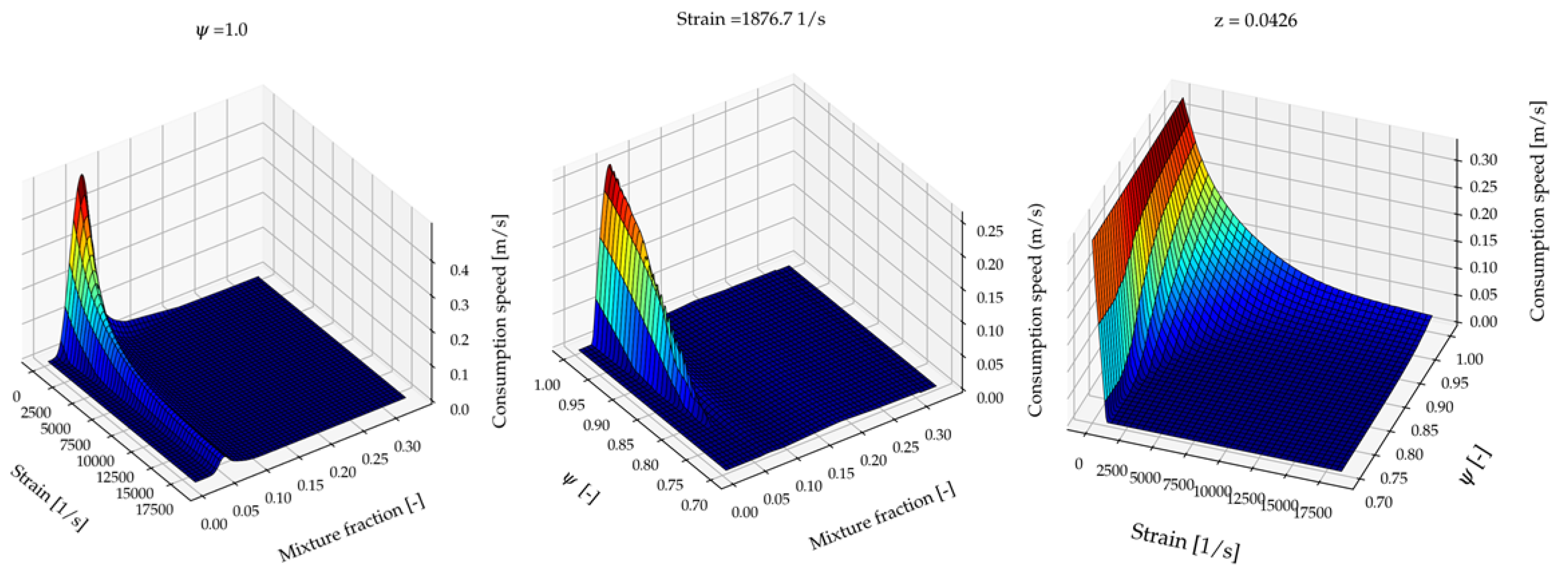
This term is evaluated from laminar simulations, and it has shown that it assumes a constant value considering the type of fuel and the operating conditions [34]. The effects of stretch and heat loss on the consumption speed can be observed in Figure 1, where isosurfaces of are reported at a fixed value of strain, heat loss, and mixture composition. While is derived from the FGM look-up table, is computed a priori and stored in an additional table. This latter tabulation is obtained from one-dimensional laminar flames considering premixed counterflow flamelets (i.e., fresh to equilibrium products) with the Cantera v2.4.0 libraries [36] and stored in an additional table. Stretch and heat loss are imposed, respectively, by varying the velocity of the opposed jets and the temperature of the burnt gas side. At run-time, this table is accessed using the stretch and the heat loss values computed in the CFD simulation other than the local composition. In this work, the consumption speed table consists of points, respectively, of z, , and .
The differences between the heat loss modeling adopted in the present work (other than in the ones in [13,37]) and the works by Tay-Wo-Chong and Klarmann with their respective co-workers are due to two aspects. First, since the use of the LES turbulence modeling context is adopted here, a different formulation for the computation of the aerodynamic stretch is required: this is expressed as , where a stands for the computed strain rate and for the curvature of the flame front. In turn, the stain rate is decomposed into two terms as , which are respectively, the resolved strain and the contribution of the sub-grid scales . For the sake of brevity, the complete formulation of these two terms and the flame front curvature is not reported here, but it can be found in [13].
The other key quantity, the heat loss parameter, requires instead some further clarifications concerning its computation. First of all, it should be noticed that the heat loss imposed in the 1D flame simulation for computing the table is modeled through the temperature of the burnt gas (i.e., c = 1 side) in the counterflow flamelets, as reported previously. This approach is the same as that employed by Tay-Wo-Chong et al., as well as Klarmann et al., Tang and Raman, and other works in the literature [24,25,28,29,33,34,35]. What differs from these works is how the heat loss is computed within the CFD calculations for the querying of the table for the consumption speed in strained and non-adiabatic conditions. Here, the heat loss parameter has to be adapted to the tabulated chemistry approach with respect to the definition used in the 1D simulations. Indeed, the heat loss here refers to the products of the laminar counterflow flamelets, which means and . In the CFD, instead, it should be formulated accordingly to the overall progress variable field, so it is expressed as the ratio of the local temperature to the local adiabatic temperature:
It can be seen that with this definition, in the fresh mixture, since here and . This fact will be explained later in the results section, where the field always assumes a value close to 1 in the swirling jet near the nozzle outlet, which is dominated by the fresh mixture. In addition, in the corners, low values of are reached, since here the local temperature is considerably far from the associated adiabatic flame temperature. Concerning the works in the literature by Tay and Klarmann, the heat loss parameter was instead defined with the enthalpy defect , where h is the local enthalpy and is the one from the look-up table. This fact was already identified in [13], and the authors consider the two approaches equivalent in the framework of non-adiabatic FGM, since the thermochemical quantities are included in the manifold as a function of the enthalpy defect with respect to adiabatic conditions. Furthermore, the fact that the present definition is adimensionalized does not represent an issue, since it is used only as a parameter to access the additional consumption speed table.
4.3. TF Model
In the Artificially Thickened Flame model [38], or most commonly, just the Thickened Flame (TF) model, no assumptions on the combustion regime are made a priori and the flame front is directly resolved. For this reason, one transport equation for each chemical species involved is present. The problem when trying to resolve the flame structures is that the flame front is considerably smaller than the usual mesh grid size: the thickening procedure alters the flame front in order to be solved on the actual mesh grid. During this operation, the correct laminar flame speed is preserved by increasing the thermal diffusivity and decreasing proportionally the reaction rate through the introduction of a thickening factor F, which is a function of the mesh grid size and the laminar flame thickness :
N is instead the number of points into which the flame front is discretized, which is set to 8 in this work. This operation, however, affects the interaction between chemistry and turbulence, since the eddies smaller than the thickened front are not interacting properly with the flame [39]. In order to mitigate this issue, the reaction rates and the thermal diffusivity are multiplied by the efficiency function E, defined as the ratio of the flame-wrinkling factors for the original flame and the thickened one: here, E is computed following the formulation given by Colin et al. [38]. Furthermore, since the thickening procedure could lead to erroneous mixing and heat-transfer, the flame is dynamically thickened only in the proximity of the flame front, through the use of a flame sensor , assuming its value is equal to 1 in the regions of interest and 0 away from them [40]. All the reaction rates in the species transport equations and the source term in the energy equation are therefore multiplied by as follows:
where is the source term of the generic species evaluated with the Arrhenius law as . The species diffusivities are dynamically computed instead as , where is the laminar diffusivity and is the turbulent one. In this fashion, near the flame, is equal to 1, and hence the turbulent diffusivities are neglected while the laminar diffusitivies are enhanced by . Instead, away from the reaction front, the expression is retrieved, and thickening is switched off. This approach has been widely applied in the literature for both premixed and non-premixed flames [40] and nowadays is one of the most popular approaches for combustion modeling concerning scale-resolving simulations.
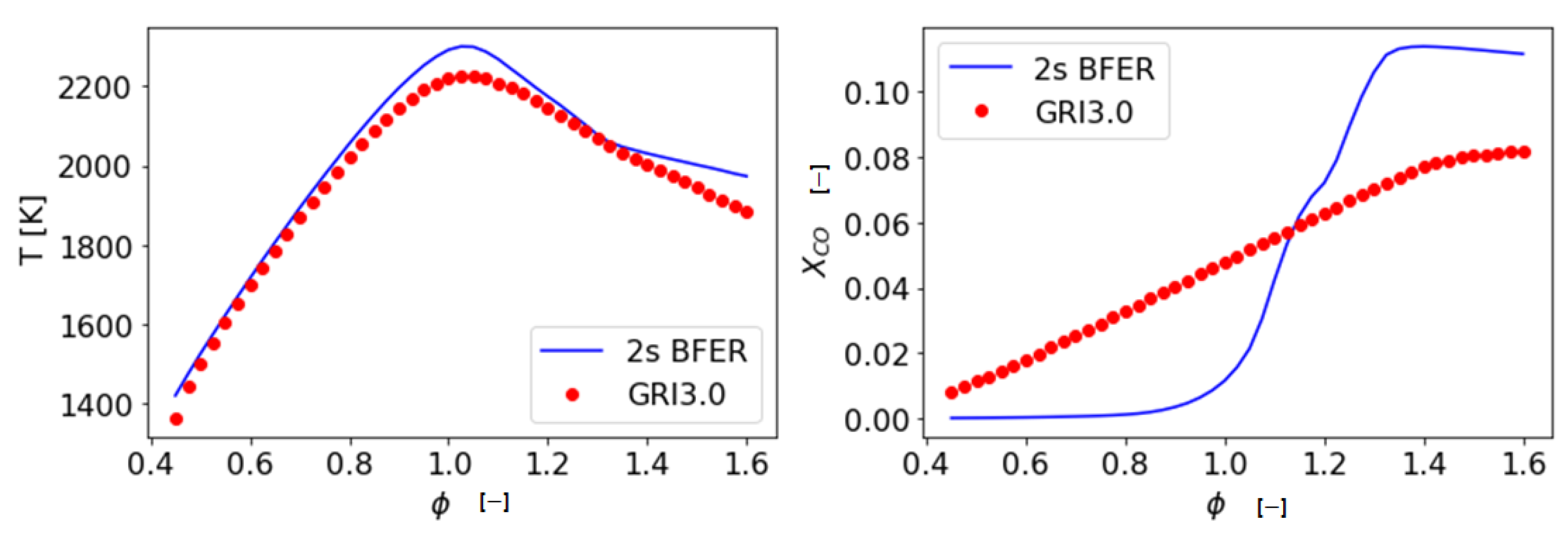
The TF model is often used together with global or semi-global [41] chemical mechanisms to reduce the number of transported species, therefore mitigating the required computational effort. In this first attempt, to apply the TF model to the Fokaides test case, the BFER 2-step mechanism for air–methane mixtures developed by Franzelli et al. [42] was used. This reaction mechanism considered six species with a first reaction concerning the oxidation of the fuel into carbon monoxide, while the second reaction took into account the final CO-CO2 equilibrium. This mechanism has been largely employed in the literature considering the LES modeling context, showing how it could successfully predict the fuel oxidation and the temperature field in the combustion chamber. However, as many reduced mechanisms, the underlying idea is to carry out a correct estimation of the laminar flame speed and adiabatic flame temperature, rather than the concentration of the intermediate chemical species [41] or potential autoignition phenomena [43]. Especially considering CO prediction, poor agreement is expected in comparison with a more detailed mechanism from a quantitative point of view: this fact can be seen in Figure 2, where the adiabatic temperature and the CO mole fraction are reported for the BFER and the GRI3.0 mechanisms simulated with a freely propagating 1D flame in Cantera for the operating conditions in Table 1. More details concerning these aspects are available in [44].
5. Numerical Setup
The numerical investigation was conducted within the LES context in order to provide a proper description of the turbulent structures present in the flow-field. Spatially filtered compressible Navier–Stokes equations were employed within the CFD suite ANSYS Fluent 2019-R1 [20]. Spatial and temporal discretization adopted second-order schemes while the Dynamic Smagorinsky–Lilly model [45] was used for the subgrid stress tensor.
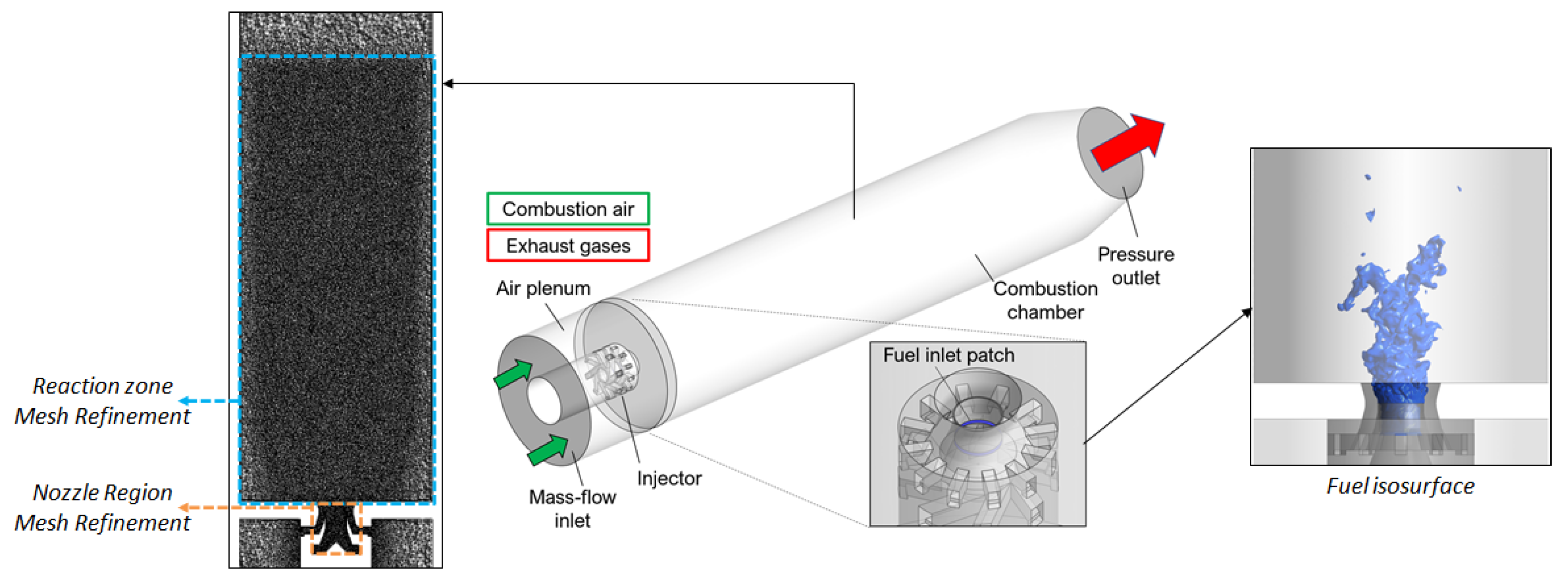
The numerical domain, reported in Figure 3, was derived from the simulations in [13], where an injector with the same configuration but lower effective area was employed. This domain includes the whole combustion chamber, together with the nozzle and the air plenum before it. A convergent section to mimic the experimental setup was placed at the outlet, aiming to prevent exhaust recirculation. The previous study investigated both isothermal and reactive conditions, and a good agreement was obtained between numerical results and experimental data for the flow-field in cold conditions. Therefore, here, the efforts have been focused on the only reactive point to assess the differences among the combustion models, assuming that the numerical setup can properly reproduce the flow structures when no reaction is occurring.
One of the main challenges of the present test case is the large extension of the reaction zone and its interaction with the confinement walls, which imposes a wide region with local refinement and thus limits the magnitude of the refinement itself. It is worth recalling at this point that this numerical study aims to investigate how different combustion models reproduce the flame characteristics. Therefore, a robust and affordable computational grid is required at this stage, while a complete study comprehensive of mesh sensitivity focusing on a single combustion model is left for future works. Keeping this in mind, an unstructured polyhedral mesh with 16 million elements was employed, since it is considered a good compromise in terms of both computational efforts and accuracy. Two distinct refinement regions were present: one within the swirler and the other in the flame tube (see Figure 3). The latter region had a maximum diameter of 85 mm for both the FGM simulations, while it reached the chamber walls for the TF model. As a result, a different mesh sizing for these simulations was used in order to meet the target overall number of elements. Therefore, the FGM models employed 250 m in the swirler and 500 m in the flame tube, while the TF model considers, respectively, 500 m and 600 m. This helps to avoid too large a value of F in the reaction zone, leading to a better reproduction of the turbulence effects on the flame front. Finally, both the setups included five prismatic layers for near-wall treatment. The study in [13] adopted a coarser mesh than the actual employed here, but still, quite reasonable results for both mean and fluctuating components of the velocity were obtained in isothermal conditions: therefore, it is assumed that at least the same accuracy could be retrieved within this work.
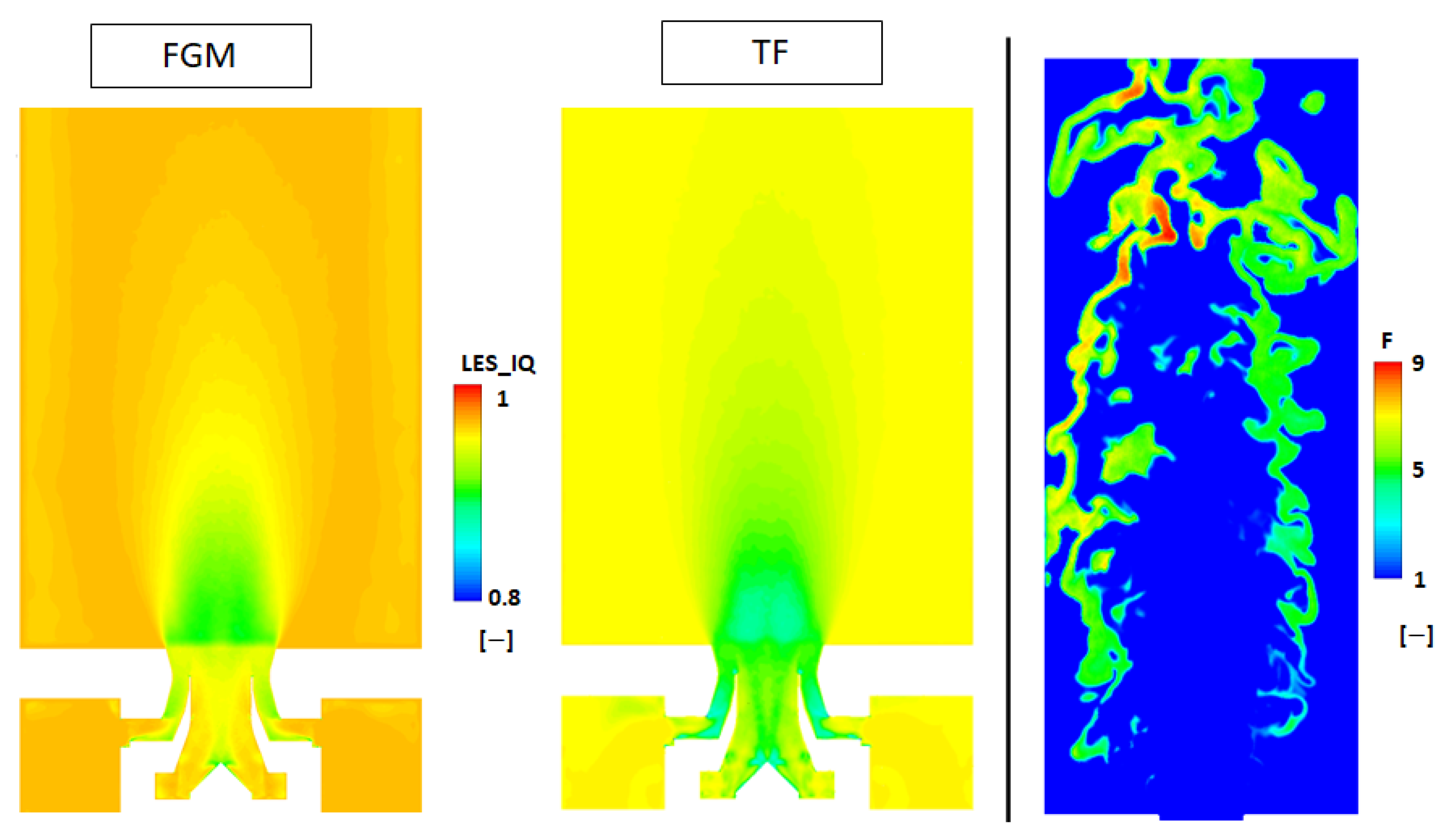
A preliminary estimation of the calculation grid adequacy was carried out with the LES Quality Index by Celik [46], where the capability of both the mesh grids to properly describe the flow-structures was assessed when a value greater or equal to was obtained. Clearly, this is not a substitute for a mesh sensitivity study, but still, it represents a preliminary indicator of mesh adequacy within the scientific community [47], especially when dealing with a test case that has not been investigated widely before; therefore, little experience is available concerning its numerical modeling (e.g., maximum element size within the nozzle for an acceptable turbulent field description). With this in mind, in Figure 4, it can be observed that the criterion is met in the whole domain for both the configurations, where clearly the lowest values are present at the nozzle exit.
Instead, focusing on the Thickened Flame approach, another important indicator of the mesh adequacy concerning the operating condition is the magnitude of the thickening Factor F. When this quantity is too large, it could lead to an improper description of the turbulence chemistry interaction, as introduced earlier when discussing this combustion model. Since the present work, as far as the authors are aware, represents the first attempt to apply the Thickened Flame model to this burner, particular attention has been paid to reproduce the acceptable magnitude of F. In this fashion, the actual mesh grid seems aligned with the value for F suggested in the literature [39]. This can be observed in the contour map, where F is reported again in Figure 4, where the largest parts of the structures assume a value of 5, while some peak values are present for such pockets of gas with richer composition (i.e., smaller laminar flame thickness).
Concerning the boundary conditions, a mass-flow inlet was used for the air plenum, while a pressure outlet was present at the outlet: here, the ambient pressure was imposed according to the conditions reported in Table 1. Fuel injection took place before the prefilmer lip with a dedicated inlet patch where its mass flow was derived accordingly to the global equivalence ratio. Concerning the walls of the combustion chamber, a no-slip condition was used for the relative boundaries in all the simulations.
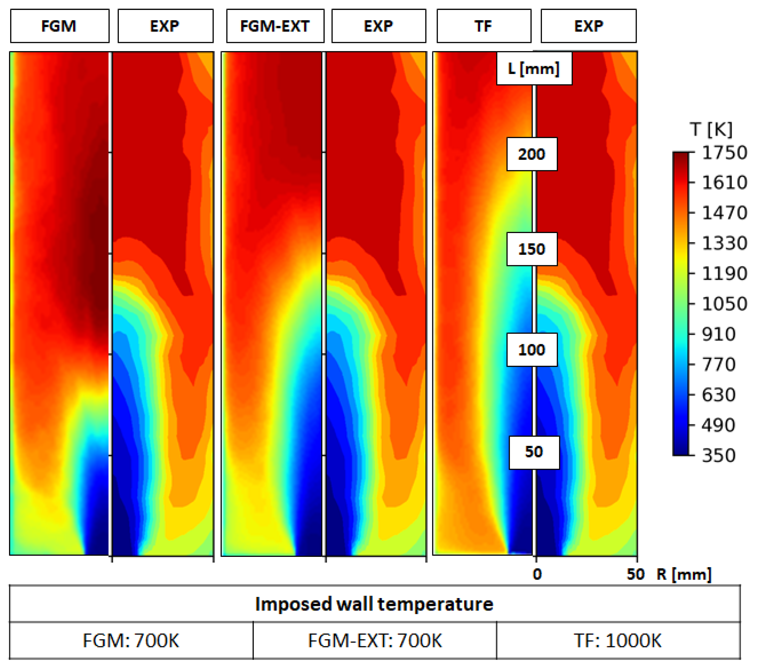
Instead, the modeling of the thermal boundary condition on the lateral and bottom walls was a challenging aspect to take care of. Firstly, no accurate information is available concerning the wall temperature from the experimental campaign. In this fashion, two different wall temperatures were used for, respectively, the FGM and the FGM-EXT models and the TF one, namely 700 K and 1000 K. This choice might appear counterintuitive since this study should assess the impact of the combustion modeling on the flame representation. However, doing this allows the magnitude of the heat losses through the walls to be maximized in the FGM simulations but still with a reasonable value of temperature. Indeed, as will be shown in the results section, this temperature matches well the experiments near the dome of the combustion chamber: assuming an even lower temperature might be unrealistic considering the test rig setup and operating conditions.
With this in mind, the FGM-EXT approach should provide a good agreement with the flame or even the flame quench in the extreme case. In other words, this strategy should highlight the fact that the potential misprediction of the flame lift-off is due to an actual limit of the combustion model, rather than a low magnitude of the heat losses through the walls. This wall temperature was initially also imposed in the TF simulation (not reported here for the sake of brevity), resulting in the presence of unburnt fuel pockets at the outlet section, which is not possible considering this test rig. For this reason, the wall temperature was increased to the current value of 1000 K, which is again a reasonable value considering the GT application field [25,27].
Although a well-defined sensitivity study of the wall temperature for the TF model has not been carried out, as will be explained in the results section, this higher wall temperature already leads to a good agreement with the experiments in terms of fuel concentrations maps. In this sense, the use of 700 K as the wall temperature would result in a worse prediction of the flame position. In addition, another interesting point might be the scenario if a wall temperature equal to 1000 K is also applied to the FGM and FGM-EXT approaches. At a first look, it is expected that the FGM-EXT will not revert to the FGM, since even if the heat loss magnitude is reduced, the correction effects might be negligible only in the absence of stretch actions, as visible in Figure 1. Further comments will be given in the dedicated results section.
The time step was set to 1 × 10 s, with a CFL value below 5 in the whole domain and below 0.5 in the flame region. The simulated physical time for each simulation is therefore reported in Table 2, where the Flow-Through Time (FTT) is preliminarily estimated from the experimental measurements window and the average flow-velocity from the same measurements.
6. Results
6.1. Flow-Field and Local Mixture Composition
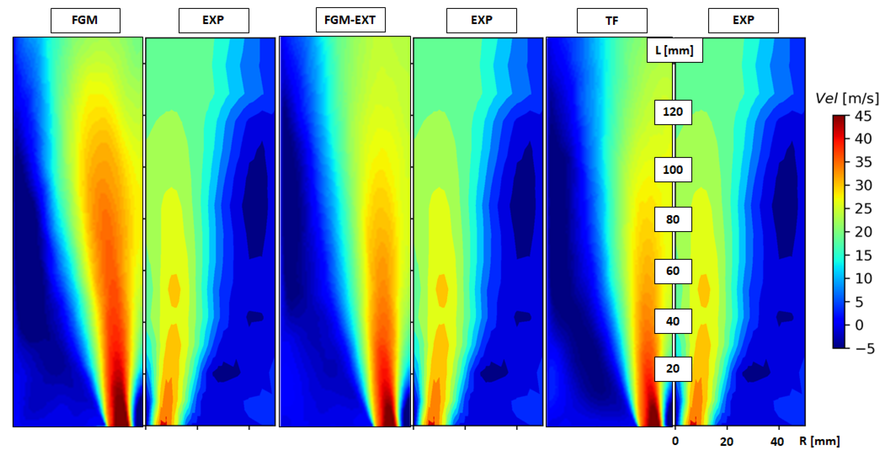
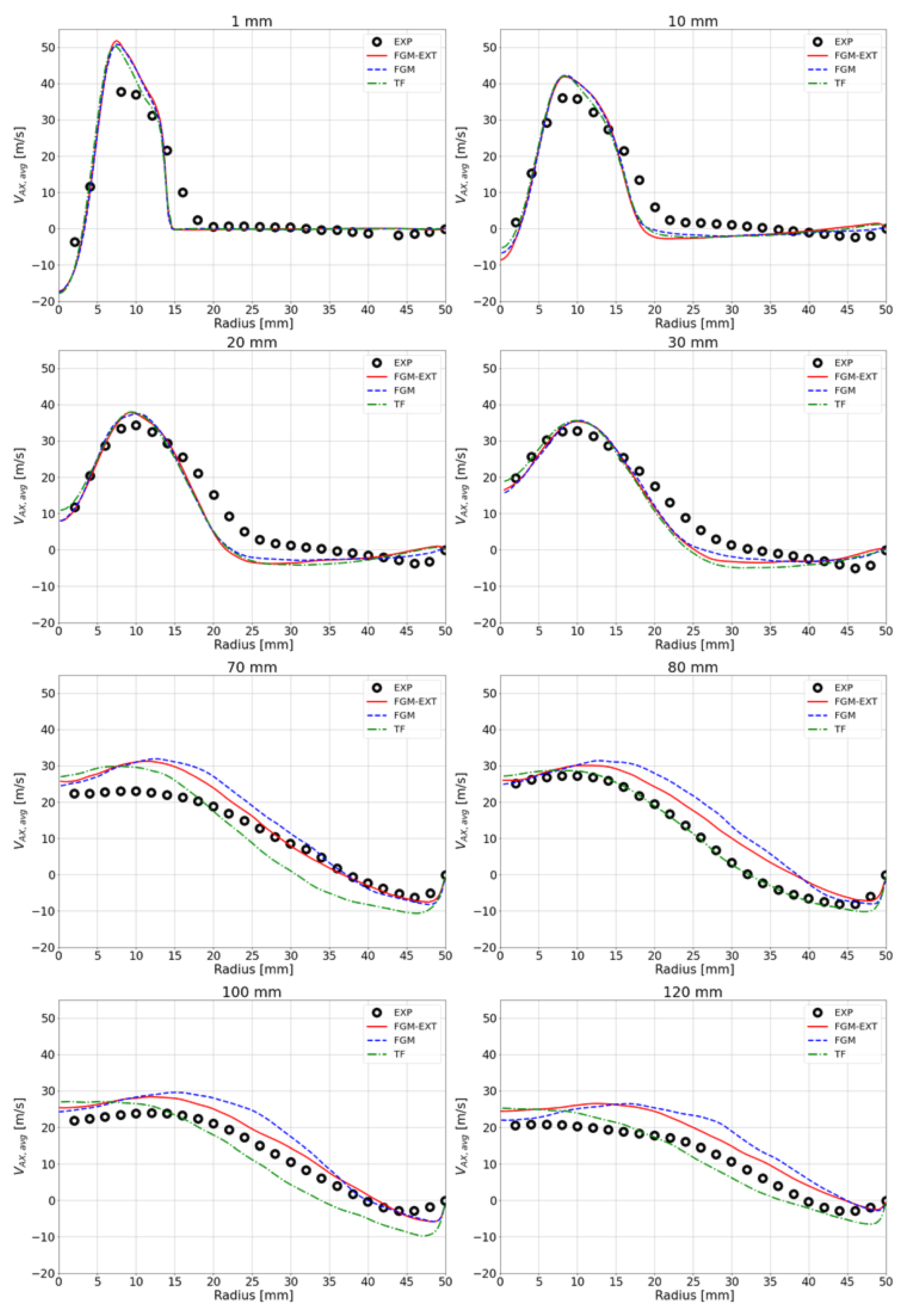
As mentioned above, this type of nozzle is characterized by a low swirl number, which is responsible for a peculiar flow-field with respect to the high-swirl injectors, commonly employed in the current GTs application. In Figure 5, the velocity field on the midplane up to 150 mm is reported for all the combustion models and experiments in terms of mean axial velocity maps.
From a qualitative point of view, the results are in good agreement with the experimental data since all the key features can be observed, regardless of the specific combustion model. These involve the high-velocity streams close to the burner axis and rapidly decaying away from it in the radial direction, as well as the almost absent IRZ. Furthermore, the wide ORZ is visible along with the main jet, which extends from the burner dome into the combustion chamber. Considering this last point, here, the differences among the three combustion models are instead visible and they could be attributed to the different position of the predicted flame, hence the related thermal expansion of the flow.
A quantitative comparison is depicted in Figure 6 based on the radial profiles of axial velocity for given axial positions. Considering the nozzle near-field up to 10 mm, all the combustion models collapse on a single curve, since no influence on the flow due to the reaction zone is present yet. Here, the small IRZ is visible close to the nozzle axis, followed by a peak of velocity within 20 mm in the radial direction. Then, the axial velocity rapidly decreases, due to the presence of the ORZ. All the employed combustion models are in good agreement with the experimental data, except for the value of the peak velocity, which is overpredicted for the profile at 1 mm. Furthermore, the experiments show a larger spreading in the radial direction, while the numerical simulations somehow reproduce a sort of narrower high-velocity stream, where the velocity decays more rapidly around 15 mm. A similar conclusion can also be drawn for the profile at 20 mm and 30 mm. Instead, from 70 mm, the effects of the ongoing reaction are clearly visible, and the combustion models begin to reproduce different trends in the radial direction. As expected, when the flame is predicted in a lower position, the influence of the heat release accelerates earlier the flow: the result is a higher value of velocity. This is the case for the FGM and the FGM-EXT approaches, which are always above the corresponding curve for the TF approach.
Nevertheless, it is worth recalling that for the desired goal of this work, the flow field can be considered sufficiently described. Further improvements to the numerical model are instead left to future works.
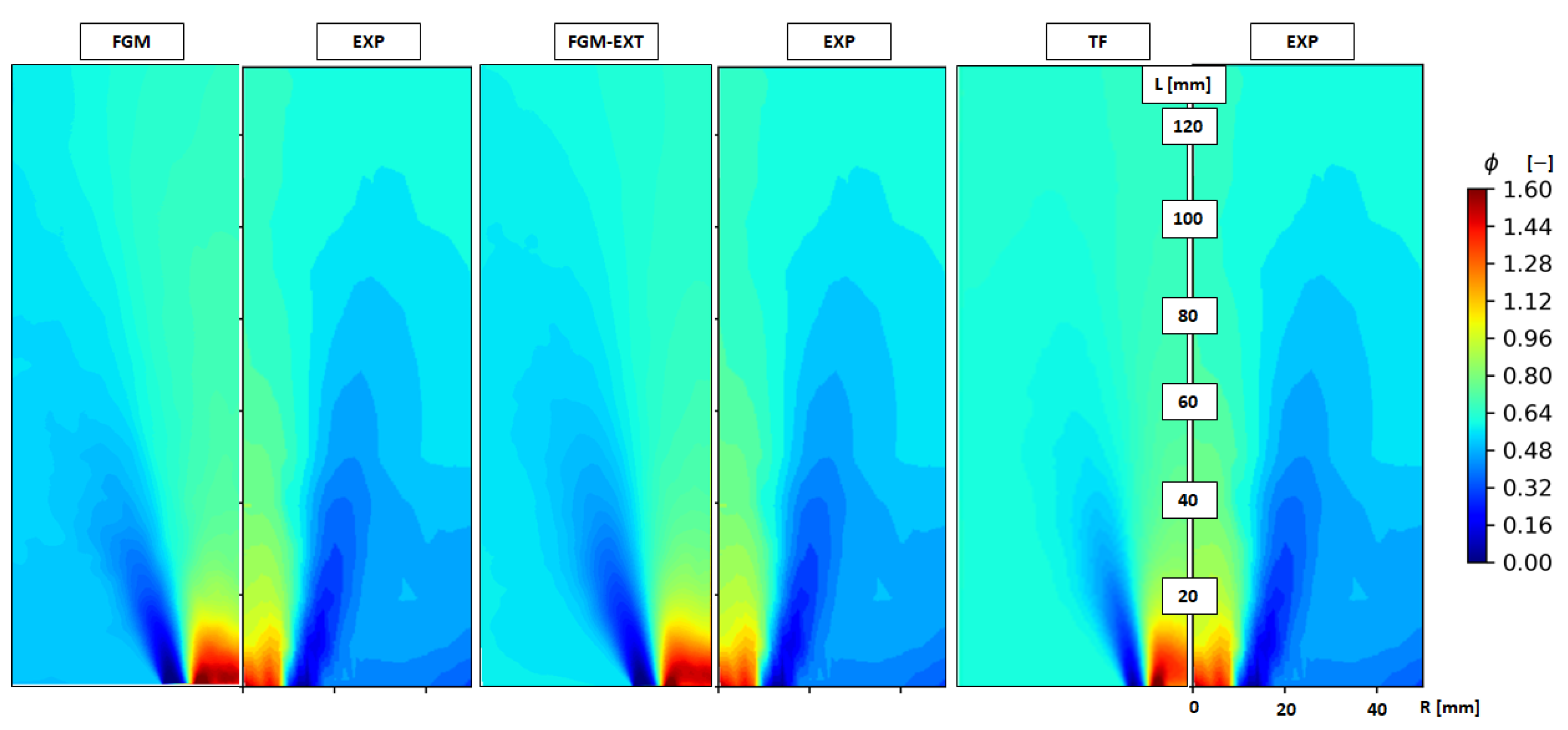
The local composition of the mixture is reported in Figure 7 in terms of equivalence ratio contour maps. This quantity accurately describes another very important characteristic of the investigated nozzle: the mixing process between air and fuel along the LOH.
Since methane is injected only in the primary swirler, a fuel-rich composition is present close to the axis at the nozzle outlet section. In addition, the pure air jets related to the secondary swirler are clearly visible at the bottom of the combustion chamber. These flow structures prevent the flame reattachment, since they avoid the interaction of the vitiated products with the fresh mixture, thus delaying the ignition. As for the velocity field, all the tested approaches are in a good agreement with the experimental data from a qualitative point of view. Furthermore, these contour maps adequately explain the driving principle of this type of flame, where air and fuel enter as separate streams at the bottom of the flame tube, while mixing is completed within 50 mm, obtaining the nominal value of . Meanwhile, it is clear here that the ORZ is dominated by vitiated air, which, as explained, is of paramount importance for the flame stabilization.
6.2. Chemical Species
The comparison between numerical simulations and experimental measurements in terms of chemical species is one of the most interesting and critical aspects considering the goal of the present work.
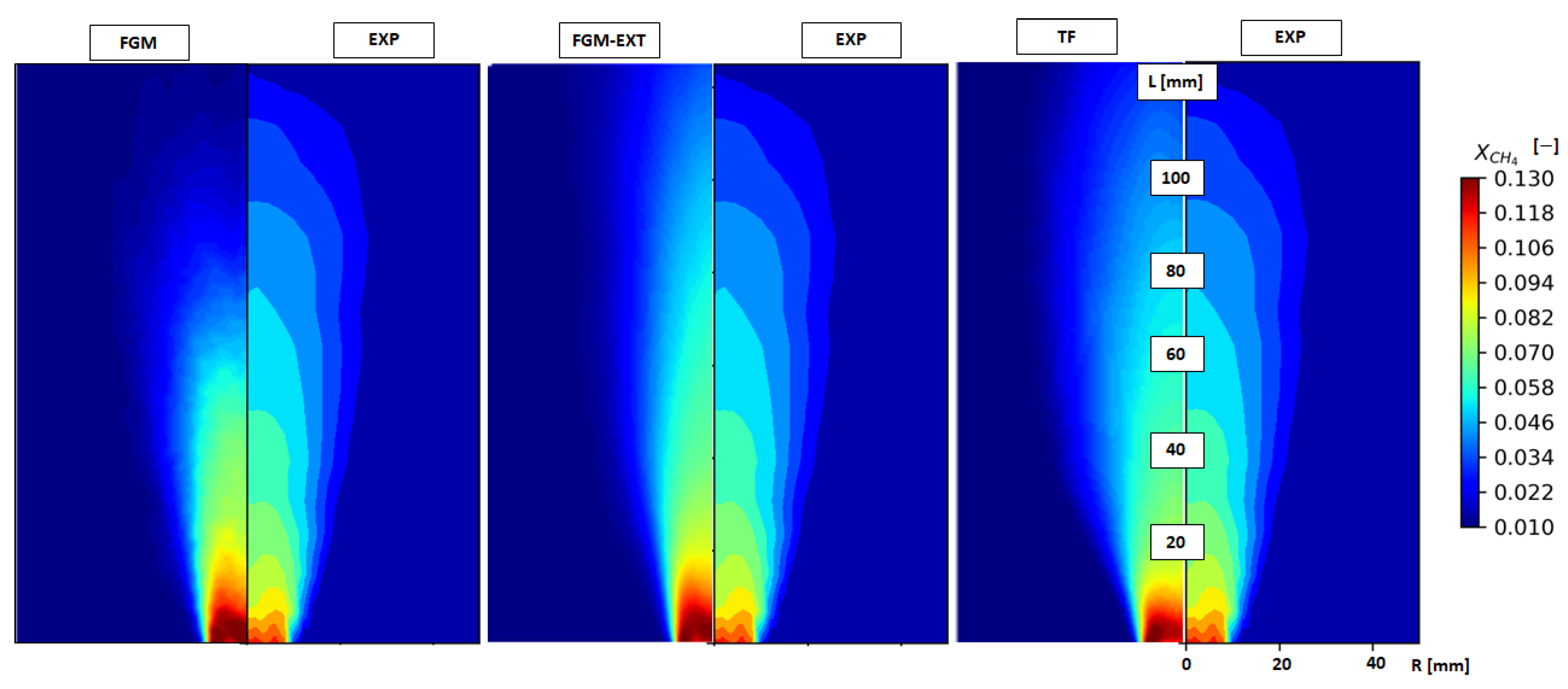
Figure 8 and Figure 9 report the comparison in terms of methane mole fraction and carbon dioxide mole fraction . In contrast to the previous equivalence ratio maps, here, the differences between the combustion models are clearly visible. Considering the maps, the FGM model reached complete oxidation of the fuel before 100 mm in the axial direction, showing the over-prediction of reactivity already seen in previous works. This issue is largely improved with the FGM-EXT approach, where the fuel oxidation is not completed in the reported 125 mm, as depicted in the experimental map. However, the levels of are lower than expected at the end of the maps, leading to an imperfect agreement with the measurements. The opposite situation is instead verified for the TF approach, where the levels of at 125 mm are slightly higher than the experimental counterpart.
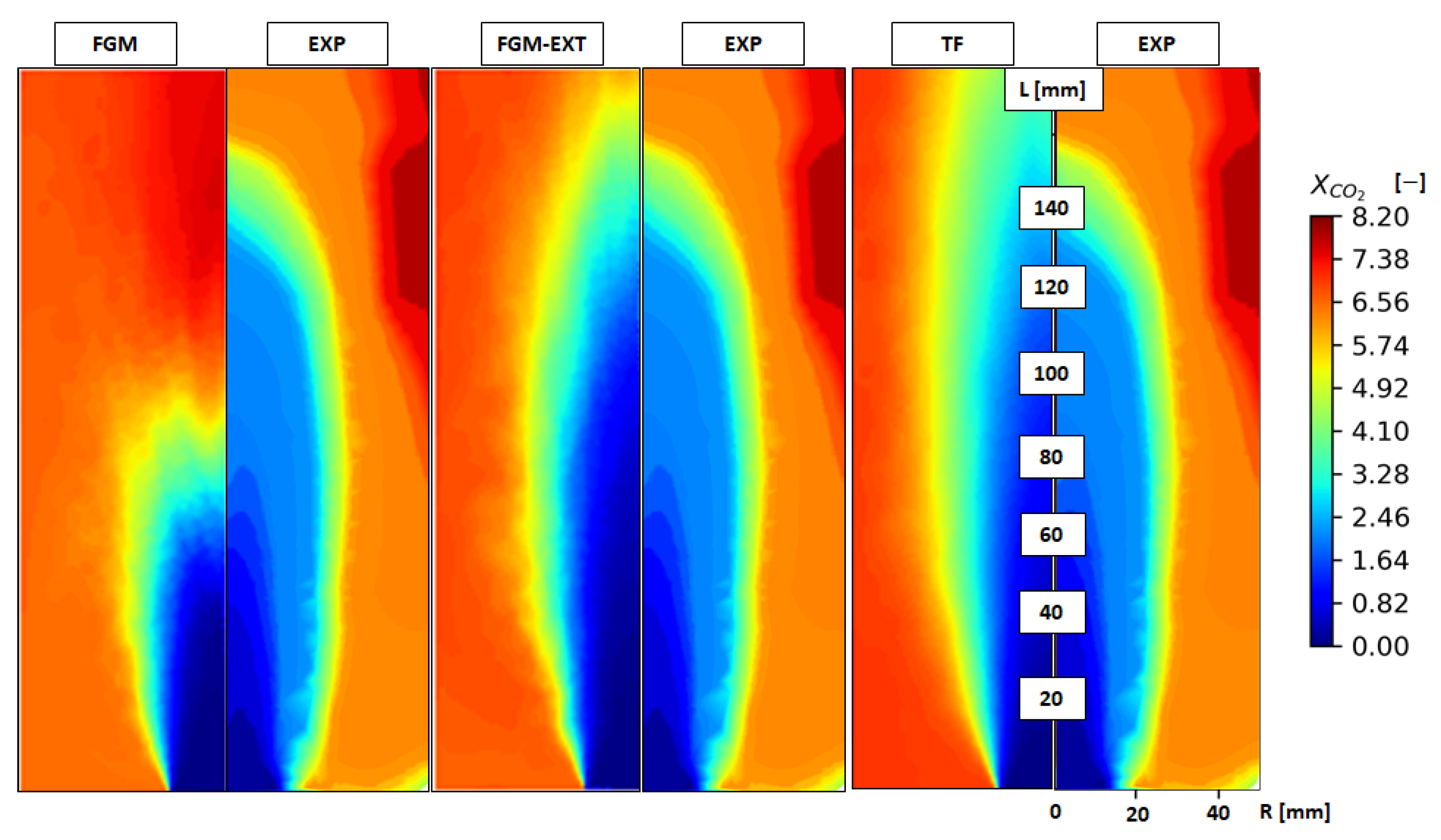
Regarding the contour maps of carbon dioxide mole fraction , the inner region of the swirling jet is dominated by low values, since no reaction is yet occurring here and the high velocity streams avoid the presence of recirculating combustion products. Again, the FGM model reproduces a small penetration of the nozzle jet, rapidly approaching the values of corresponding to the equilibrium composition. The FGM-EXT and the TF models are instead comparable from this point of view. The concentration of CO instead reaches high levels in the ORZ, due to the presence of combustion products. Furthermore, the experimental contours are reporting lower levels of at the bottom of the flame tube that are not predicted in the numerical simulations: this aspect will be further investigated in future works.
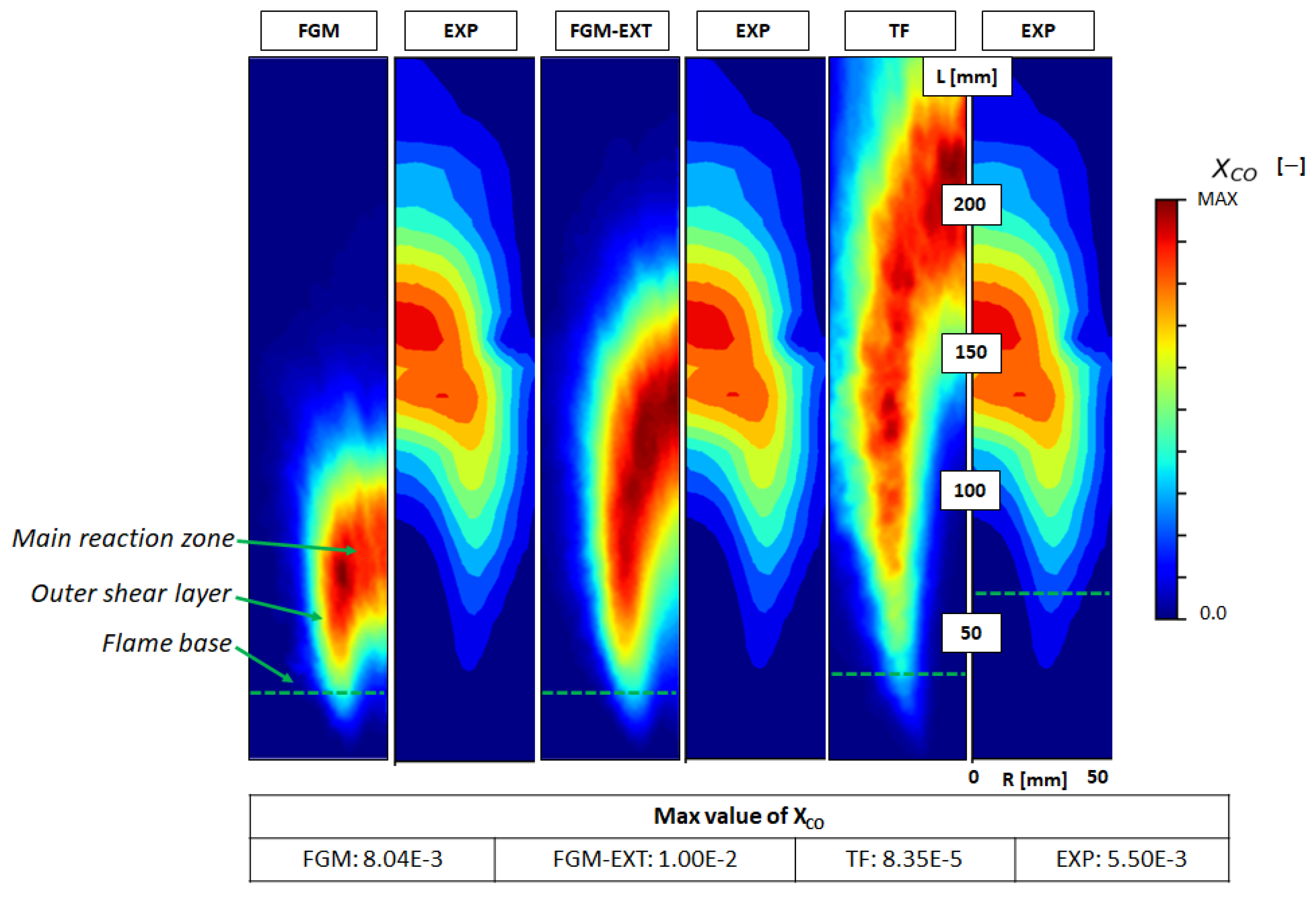
Figure 10 reports the mean carbon monoxide mole fraction, , which can be considered a good indicator of the ongoing reaction from a qualitative point of view. Each map refers to the maximum value observed on this plane for a specific combustion model: these are reported in the related table again in Figure 10. It can be seen that the TF simulation underestimates the peak by two orders of magnitude with respect to the experimental finding, while both FGM models instead overestimate this value but within almost the same order of magnitude. This fact could be explained by the previously mentioned misprediction related to the two-step chemistry, which is reported also in [44]. Nevertheless, from a qualitative point of view, this comparison permits the visualization of the flame region in terms of extension and shape.
The lift-off occurrence is predicted by all the combustion models, since each map reports the reaction zones detached from the nozzle outlet. As found in [13], the FGM model reproduces a short and more compact flame than the experiments. The main reaction zone is found between 50 and 100 mm, while the flame base occurrence can be found around 25 mm. However, the flame assumes an arrow shape, where the anchoring edges are visible in the outer shear layer. The FGM-EXT improves the flame prediction by taking into account the stretch and heat loss effects, even with the simple approach introduced in the combustion modeling section. Here, the main reaction zone is placed between 100 and 150 mm, making it closer to the experimental map. This is because the inner zone around the axis now experiences a lowered reactivity thanks to the intense stretch field related to the nozzle jet. Still, the LOH is underpredicted since the first occurrence of the reaction zone is almost identical to the standard FGM outcome. Furthermore, high values of , similar to the ones present in the main reaction zone near the burner axis, are found in the outer shear layer. A possible explanation for this is related to the stretch field presence, which assumes very low values in the ORZ and decays moving downstream in the flame tube, as will be shown in the next section. Differently from the TF model, the main reaction zone stabilizes around 200 mm, which is even further downstream from the experimental finding (i.e., 150 mm). The flame again assumes all the features already seen with the other models in terms of anchoring edges, arrow shape, and inner regions devoid of reactions, but all these zones now have a larger extension. Another important point to highlight is that the reaction zone now reaches the lateral confinement walls, which is reported also by the experimental map, and could potentially enhance the heat losses contribution. This aspect was observed also by Sedlmaier in [11], where the impact of different cooling flow rates was tested: in particular, a non-linear behavior of the LOH with the increase of cooling flow rate occurred when the flame interacted with the walls. Unexpectedly, the base of the flame is still placed in the lower zone of the combustion chamber, and it is closer to the FGM models rather than the experiments. The latter indeed is anchored beyond 50 mm, while the TF model reactions occur before this position.
6.3. Temperature Field
The comparison between numerical simulations and experiments is reported in terms of the temperature field in Figure 11. As mentioned in the numerical setup section, the FGM models and the TF employ different values of wall temperature, since imposing 700 K for the TF simulation results in the presence of unburnt fuel at the outlet, which is not the case considering the experimental findings. All the contour maps showing a relatively cold region close to the nozzle axis corresponding with the swirling jet, while a higher temperature is present in the ORZ dominated by the combustion product recirculation. The extension of this cold region depends on the combustion models, since it is strictly related to the position of the main reaction zone, as shown by the maps. Although the best prediction in terms of is related to the higher value of wall temperature, the temperature field in the FGM models reaches a better agreement with the experiments near the bottom of the flame tube. In addition, the region with the highest temperature (close to the adiabatic flame one), according to the experimental map, seems better described in terms of its position with the FGM-EXT model rather than the TF one. Besides the value imposed on the walls, it is expected that a uniform wall temperature could lead to a wrong prediction of the flame temperature field. This means that the wall temperature set to 700 K is likely reasonable for the first part of the combustion chamber, as shown in Figure 11, but then this value should be increased by taking into account the heat transfer with the recirculating products, similar to the strategy reported by Massey et al. in [27]. This aspect is clearly of primary importance and will be investigated in detail in future works.
Another important consideration that can be drawn is that the misprediction associated with the FGM and the FGM-EXT approach is not related to improper wall thermal boundary conditions, but an actual limit of this type of modeling. Indeed, the lower wall temperature should have enhanced the effect of , thus predicting a reaction zone with the FGM-EXT closer to the experimental measurements with respect to the TF model.
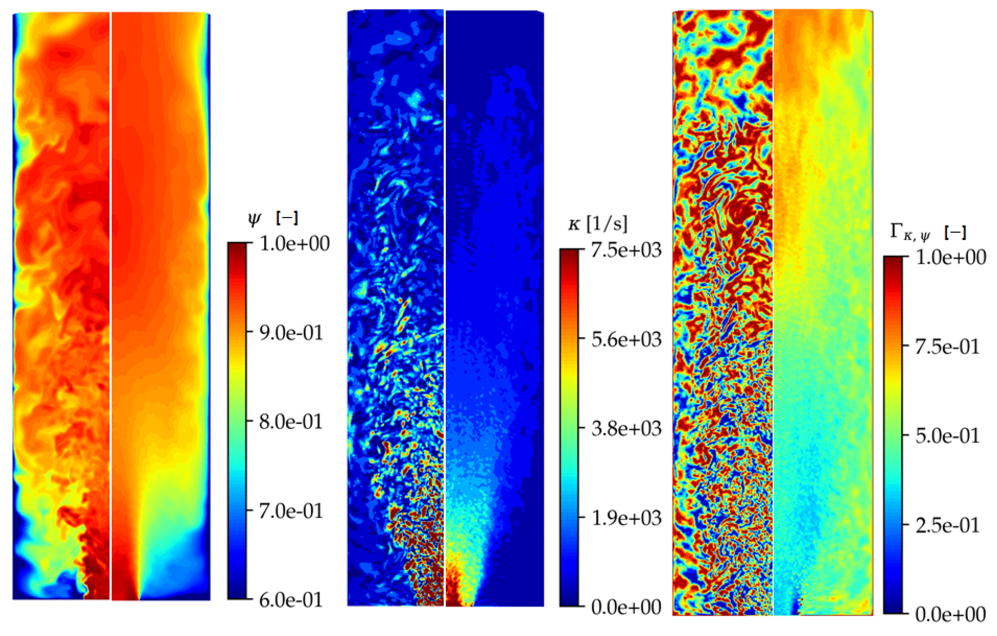
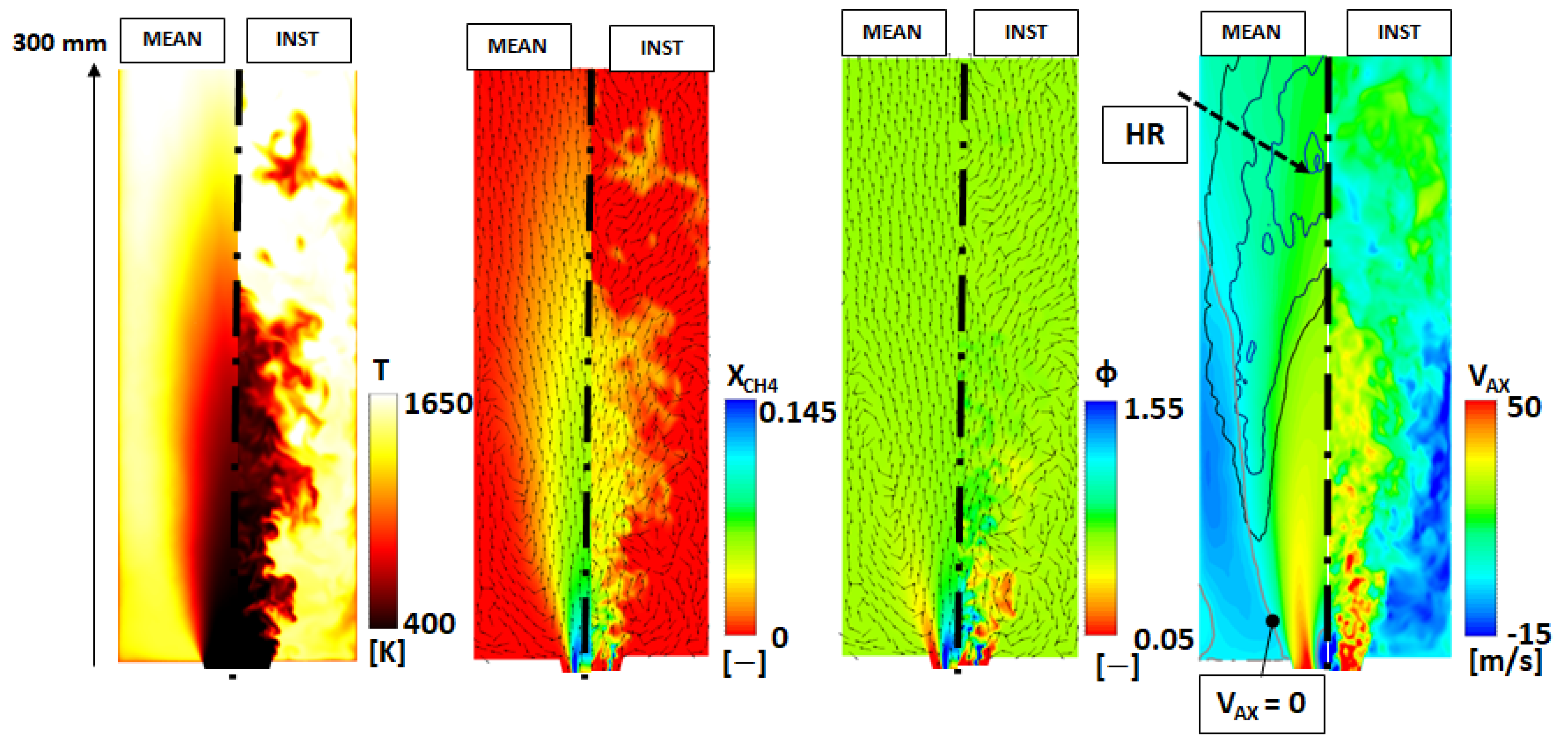
A better understanding of how the heat loss correction works in the FGM-EXT is possible thanks to Figure 12, where the instantaneous and mean fields of heat loss , stretch , and correction factor are reported. As explained previously, directly affects the global reaction rate in the FGM-EXT: the regions distinguished by low values are the ones where the flame experiences a reactivity decrease and potentially a local quench. The value of depends on the local level of aerodynamic stretch and heat loss. The first reaches high values in the nozzle near field and close to the burner axis. The heat losses instead are concentrated in the bottom corner of the combustion chamber and near the confinement walls. This means that the low temperature imposed at the walls for the FGM-EXT enhances this quantity, as visible in Figure 12. For this reason, even if a relatively strong heat loss field is present in the corners, the low values assumed by the stretch field maintain a reduction factor at an intermediate level, which can also be deduced from Figure 1. Furthermore, the chaotic behavior of the instantaneous field of is again related to the same field of , which is governed by the turbulent structures in the flow.
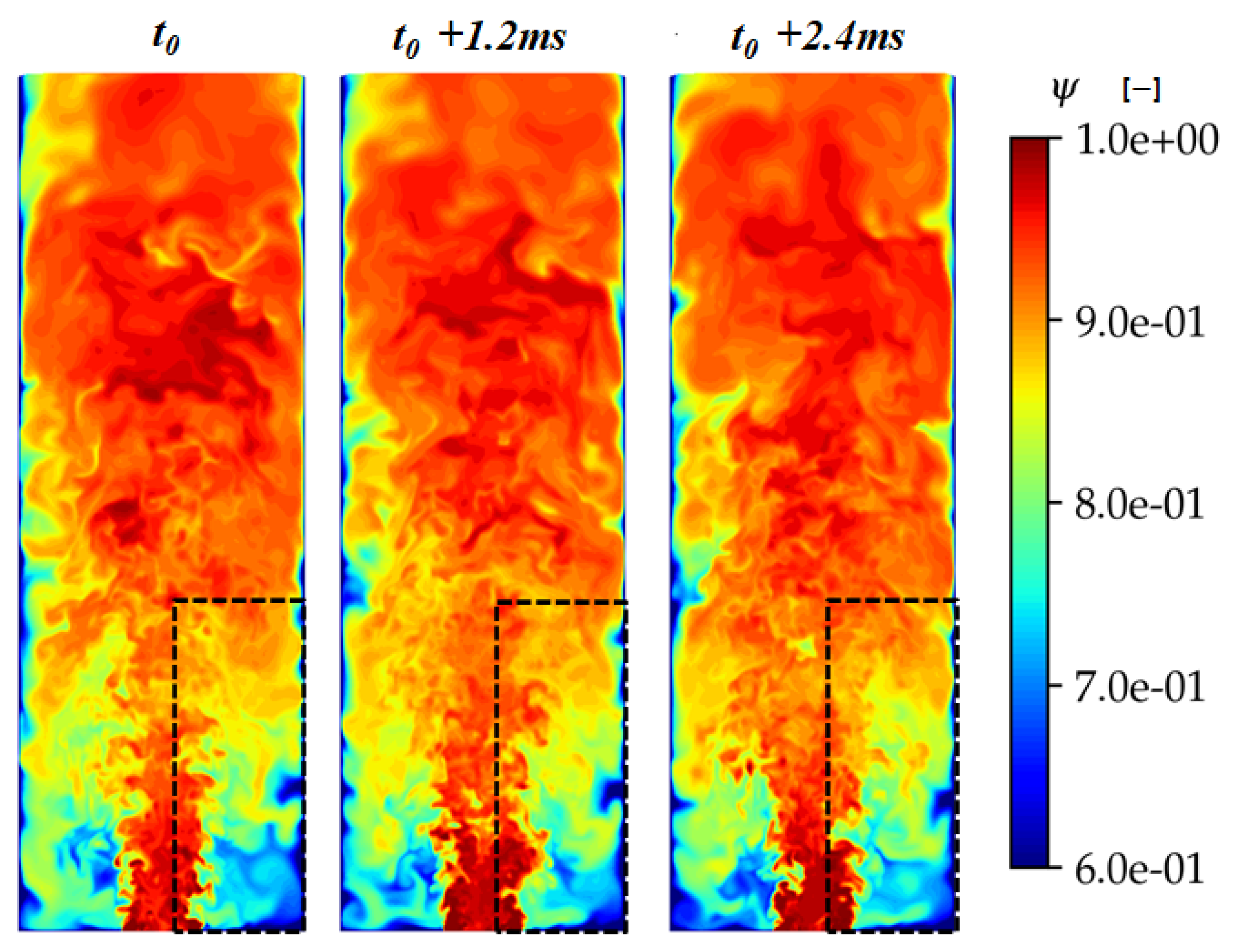
Moreover, the importance of the wall heat losses can be deduced by considering the sequence in Figure 13 reporting the instantaneous field of for various instants of time. It is worth recalling that for this simulation, the wall temperature is imposed to be 700 K, which is less than half of the adiabatic flame temperature; therefore, the heat loss will be strongly enhanced at the walls. The hot combustion products are taken from the reaction zone upstream and transported by the ORZ upstream toward the bottom of the flame tube. During this transport, as highlighted with the black dashed lines in Figure 13, these gases are cooled down by the walls, thus delaying the ignition of the incoming fresh mixture.
7. Considerations on the Stabilization Mechanism
In Figure 14, the mean and instantaneous contours for the TF simulation are reported in terms of the temperature, methane mole fraction, equivalence ratio, and axial velocity field: in the latter contours, isolines of heat-release and zero axial velocity are superimposed. The flame stabilizes at a position where a sufficiently low value of the velocity is reached: this can be seen by both the decrease in methane concentration as well as the increase in mean temperature in the flame tube along the axial direction. The flame base is anchored on the outer shear layer of the swirling jet, as visible from the zero axial velocity isoline tangent to the heat-release ones. Furthermore, the temperature and equivalence ratio instantaneous fields show the presence of turbulent instabilities at the jet’s basis: this phenomenon leads to the entrainment of hot vitiated products in the fresh mixture jet operating the continuous re-ignition of the reactants reported in previous works in the literature [1]. The ORZ acts as a reservoir of hot combustion products, promoting the ignition mentioned before, since all the fuel here is already consumed, but the composition shows values of close to the nominal value for this test point. Similar considerations could be made concerning the FGM and the FGM-EXT, but for the sake of brevity, these models are not reported: the same comparison can be found in the previous work [13].
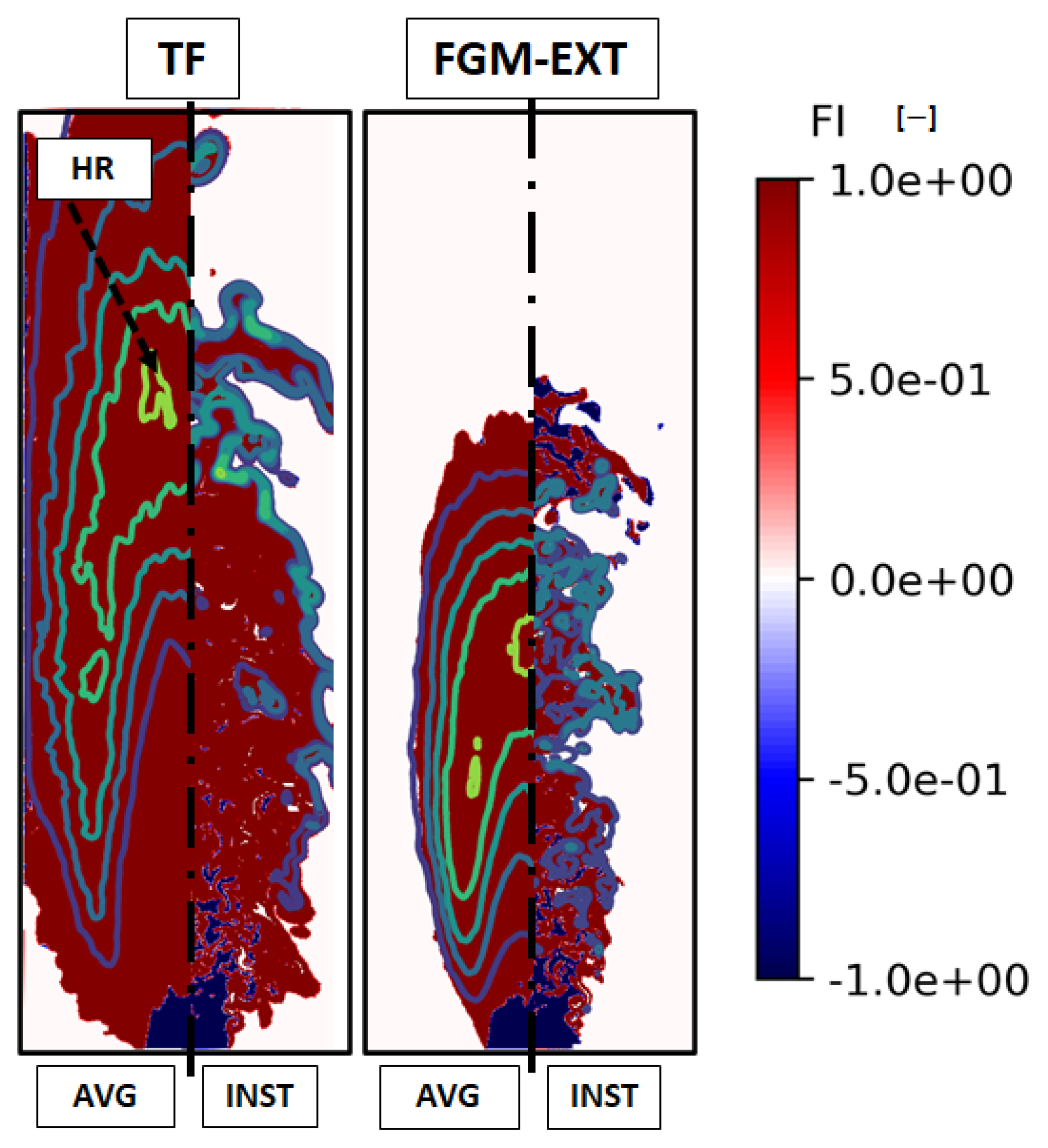
Additionally, in Figure 15, the instantaneous and mean maps of Flame Index are reported for both the TF and the FGM-EXT models, with the isolevels of heat release superimposed. The Flame Index can be interpreted as an indicator of where the flame can be assumed in a premixed state or a non-premixed one. This quantity is defined as [48]:
where a value equal to 1 indicates a premixed state of the reactive mixture and -1 as a non-premixed one. In Figure 15, it can be seen that both approaches are dominated by premixed-like conditions, since such a state is reached very early in the combustion chamber. This also highlights the capability of this low-swirl lifted flame to operate as a premixed flame without the use of premixing chambers.
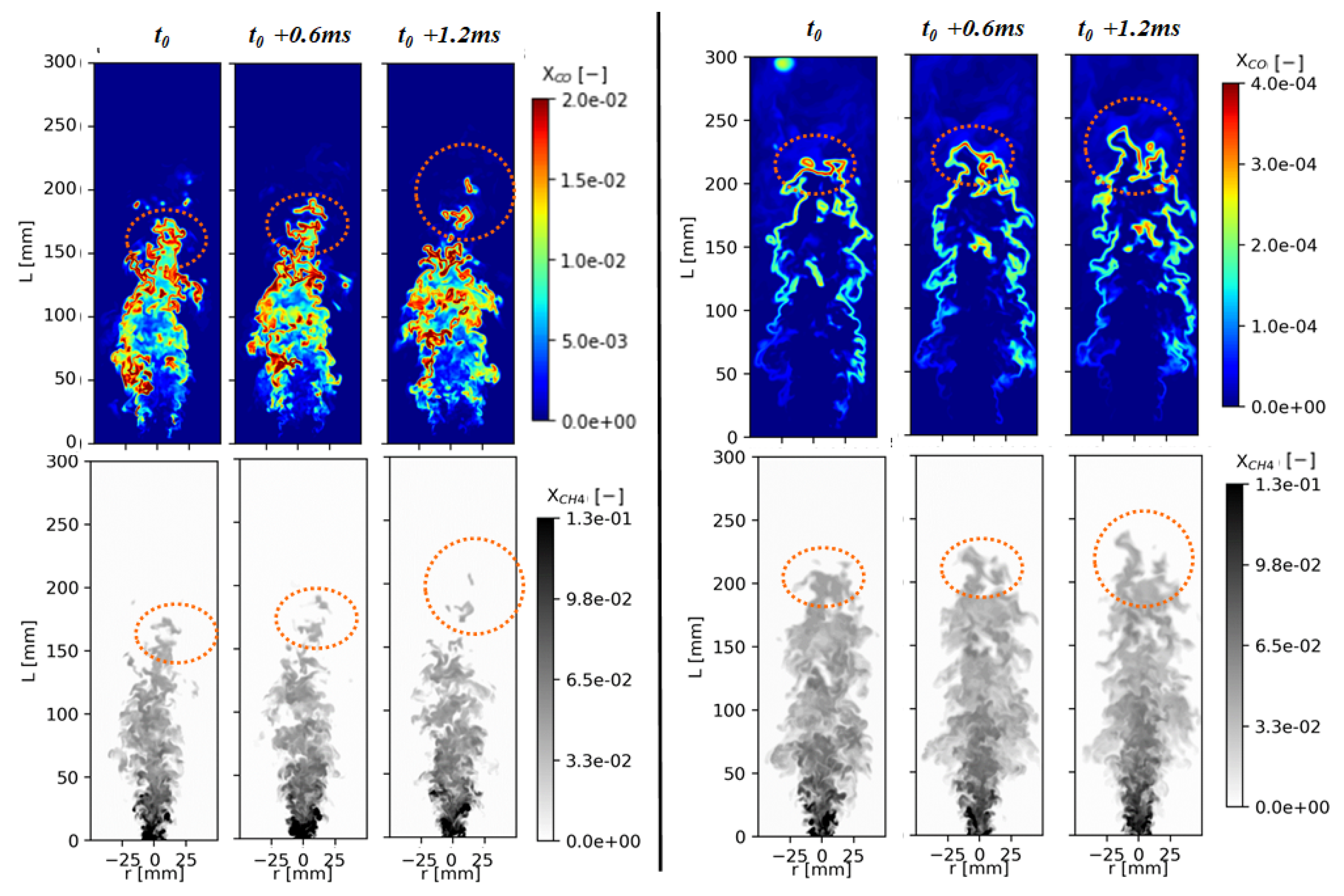
Finally, instantaneous maps for and are reported in Figure 16. Three consecutive instants are reported, aiming to show the dynamic behavior related to the reactive regions. The swirling jet enters the flame tube with a rich local composition, and it experiences the already mentioned flow instabilities interacting with the vitiated hot products and promoting the mixing downstream. The presence of carbon monoxide acts as an indication of the flame front position, showing how the fuel is being consumed. The TF simulation shows a thin reaction front that is strongly deformed by the turbulence. Moreover, it can be seen how the flame interacts with the lateral walls, which indeed enhances the heat losses and therefore the decrease in the reactivity. The reaction front surrounds the reactive mixture regions (circled in Figure 16) with a sharp and well-defined front: from a modeling point of view, this behavior is due to the dynamic thickening, and here, the flame sensor drops to 0 within this region. Instead, the FGM-EXT field reports a compact reaction zone that is highly corrugated, and this time, the direct interaction with the walls does not occur. The reactive mixture regions show a diffused reaction zone, where the higher values are present at the outer layer of this region. The flame front position is now related to the transport of the mean progress variable and its variance, where the assumption made for the turbulence–chemistry interaction plays a decisive role.
8. Conclusions
In this work, a low-swirl partially premixed lifted flame operated with gaseous fuel has been studied using LES simulations with three different combustion models. The goal is to understand which of these is the most suitable for the representation of the flame in terms of lift-off height and reproduction of the reaction zone. The employed combustion models are, respectively, the TF model, the FGM model, and finally a version of the FGM with stretch and heat loss correction.
Another crucial point is the influence of the heat losses on the final prediction, which was demonstrated with both experimental and numerical results in previous studies. Since no information on the wall temperature is present, a uniform value has been imposed on the wall’s thermal boundary conditions: this value has been chosen considering the experimental results near the bottom of the combustion chamber, similar to previous studies in the literature. This wall temperature results in a value of 700 K, which should have enhanced the effects of the heat loss correction in the modified FGM approach. Conversely, this wall temperature magnitude applied in the TF simulation has led to the presence of unburnt fuel on the outlet section, which is unrealistic considering the present test case. For this reason, in this simulation, the wall’s thermal condition is set to 1000 K. In spite of the different thermal boundary conditions, some remarks are possible considering the numerical results.
Firstly, all the models predict the flame lift-off, and all are very close to the experiments in terms of velocity field and local composition of the exhaust gas. The main differences are related to the position of the reaction zones in terms of CO mole fraction and obviously of the temperature field. The FGM models under-predict the flame height and extension, both in the axial and radial directions, despite the higher magnitude of the heat losses. The TF model instead slightly overpredicts the main reaction zone position, even with the higher wall temperature. All the models noticeably retrieve the early occurrence of reaction in the flame tube in the ORZ, which is not observed in the experiments. Furthermore, the TF model largely underpredicts the CO concentration due to the use of two-step mechanisms with respect to the FGM models employing a detailed mechanism. The temperature field is affected by the choice of the different boundary conditions: a general conclusion is therefore not possible from a comparison between combustion models, except that the use of uniform wall temperature is not correct when also considering the flame extension in the combustion chamber. Moreover, the experimental findings concerning the stabilization mechanism seem correctly reproduced by all the models, as already also observed in a previous work by the authors.
Future investigations will focus on understanding the reason behind the improved prediction of the TF model over the FGM ones. Furthermore, it should be pointed out that the stretch and heat loss correction employed here is a simplistic but cost-effective approach, while different strategies to include these effects within the FGM framework are available in the literature and should be tested before drawing certain conclusions. At the same time, the discrepancies of the TF model from the experiments should be investigated aiming to understand if this could effectively be related to the simplified chemistry description rather than an improper turbulence–chemistry interaction predicted by the model. Finally, the impact of the grid discretization should be assessed with a dedicated mesh sensitivity study aiming to verify the assumption made in the present work.
Author Contributions
Conceptualization, A.A. and L.L.; methodology, A.A.; software, L.L.; validation, L.L., M.A. and A.A.; formal analysis, L.L.; investigation, L.L. and M.A.; resources, A.A.; data curation, L.L.; writing—original draft preparation, L.L.; writing—review and editing, L.L.; visualization, A.A.; supervision, A.A.; project administration, A.A.; funding acquisition, A.A. All authors have read and agreed to the published version of the manuscript.
Funding
This project has received funding from the Clean Sky 2 Joint Undertaking (JU) under grant agreement N. 831881 (CHAiRLIFT). The JU receives support from the European Union’s Horizon 2020 research and innovation program and the Clean Sky 2 JU members other than the Union.

Data Availability Statement
The experimental data used in this study for the comparison with the numerical simulations have been provided from KIT–EBI. The numerical data presented in this study are available on request from Antonio Andreini ([email protected]).
Acknowledgments
The authors acknowledge the CINECA award under the ISCRA initiative, for the availability of high-performance computing resources. S. Harth is also gratefully acknowledged for the availability of the test rig nozzle geometry.
Conflicts of Interest
The authors declare no conflict of interest.
Abbreviations
The following abbreviations are used in this manuscript:
| FGM | Flamelet Generated Manifold model |
| FTT | Flow-Through Time |
| IRZ | Inner Recirculation Zone |
| HR | Heat Release |
| LBO | Lean Blow-Off |
| LES | Large Eddy Simulations |
| LOH | Lift-Off Height |
| ORZ | Outer Recirculation Zone |
| RANS | Reynolds Averaged Navier–Stokes |
| TF | Thickened Flame model |
References
- Lawn, C. Lifted flames on fuel jets in co-flowing air. Prog. Energy Combust. Sci. 2009, 35, 1–30. [Google Scholar] [CrossRef]
- Cabra, R.; Chen, J.Y.; Dibble, R.; Karpetis, A.; Barlow, R. Lifted methane–air jet flames in a vitiated coflow. Combust. Flame 2005, 143, 491–506. [Google Scholar] [CrossRef]
- O’Loughlin, W.; Masri, A. A new burner for studying auto-ignition in turbulent dilute sprays. Combust. Flame 2011, 158, 1577–1590. [Google Scholar] [CrossRef]
- Day, M.; Tachibana, S.; Bell, J.; Lijewski, M.; Beckner, V.; Cheng, R.K. A combined computational and experimental characterization of lean premixed turbulent low swirl laboratory flames: I. Methane flames. Combust. Flame 2012, 159, 275–290. [Google Scholar] [CrossRef]
- Fokaides, P.A.; Kasabov, P.; Zarzalis, N. Experimental Investigation of the stability mechanism and emissions of a lifted swirl nonpremixed flame. J. Eng. Gas Turbines Power 2008, 130, 011508. [Google Scholar] [CrossRef]
- Kasabov, P. Experimentelle Untersuchungen an Abgehobenen Flammen unter Druck. Ph.D. Thesis, Karlsruhe Institute of Technology, Karlsruhe, Germany, 2014. [Google Scholar]
- Fokaides, P.; Zarzalis, N. Lean blowout dynamics of a lifted stabilized, non-premixed swirl flame. In Proceedings of the Third European Combustion Meeting, Chania, Greece, 11–13 April 2007; Volume 7, p. 2. [Google Scholar]
- Kasabov, P.; Zarzalis, N.; Habisreuther, P. Experimental study on lifted flames operated with liquid kerosene at elevated pressure and stabilized by outer recirculation. Flow Turbul. Combust. 2013, 90, 605–619. [Google Scholar] [CrossRef]
- Lyons, K.M. Toward an understanding of the stabilization mechanisms of lifted turbulent jet flames: Experiments. Prog. Energy Combust. Sci. 2007, 33, 211–231. [Google Scholar] [CrossRef]
- Kern, M.; Fokaides, P.; Habisreuther, P.; Zarzalis, N. Applicability of a flamelet and a presumed jpdf 2-domain-1-step-kinetic turbulent reaction model for the simulation of a lifted swirl flame. In Turbo Expo: Power for Land, Sea, and Air; American Society of Mechanical Engineers: New York, NY, USA, 2009; Volume 48838, pp. 359–368. [Google Scholar]
- Sedlmaier, J. Numerische und Experimentelle Untersuchung einer Abgehobenen Flamme unter Druck. Ph.D. Thesis, Karlsruhe Institute of Technology, Karlsruhe, Germany, 2019. [Google Scholar]
- Langone, L.; Pampaloni, D.; Mazzei, L.; Andreini, A. Analysis of a gaseous partially premixed lifted flame in swirling flow through different LES combustion models. In Proceedings of the 10th European Combustion Meeting, Naples, Italy, 14–15 April 2021. [Google Scholar]
- Langone, L.; Sedlmaier, J.; Nassini, P.C.; Mazzei, L.; Harth, S.; Andreini, A. Numerical Modeling of Gaseous Partially Premixed Low-Swirl Lifted Flame at Elevated Pressure. In Turbo Expo: Power for Land, Sea, and Air; American Society of Mechanical Engineers: New York, NY, USA, 2020; Volume 84133, p. V04BT04A068. [Google Scholar]
- Lefebvre, A.H.; Ballal, D.R. Gas Turbine Combustion: Alternative Fuels and Emissions; CRC Press: Boca Raton, FL, USA, 2010. [Google Scholar]
- Sedlmaier, J.; Habisreuther, P.; Zarzalis, N.; Jansohn, P. Influence of liquid and gaseous fuel on lifted flames at elevated pressure stabilized by outer recirculation. In Turbo Expo: Power for Land, Sea, and Air; American Society of Mechanical Engineers: New York, NY, USA, 2014; Volume 45684, p. V04AT04A054. [Google Scholar]
- Bradley, D.; Kwa, L.; Lau, A.; Missaghi, M.; Chin, S. Laminar flamelet modeling of recirculating premixed methane and propane-air combustion. Combust. Flame 1988, 71, 109–122. [Google Scholar] [CrossRef]
- Bradley, D.; Lau, A. The mathematical modelling of premixed turbulent combustion. Pure Appl. Chem. 1990, 62, 803–814. [Google Scholar] [CrossRef]
- Van Oijen, J.; Lammers, F.; De Goey, L. Modeling of complex premixed burner systems by using flamelet-generated manifolds. Combust. Flame 2001, 127, 2124–2134. [Google Scholar] [CrossRef]
- Bilger, R. The structure of turbulent nonpremixed flames. In Symposium (International) on Combustion; Elsevier: Amsterdam, The Netherlands, 1989; Volume 22, pp. 475–488. [Google Scholar]
- ANSYS. Fluent 19.3 Theory Guide; ANSYS: Canonsburg, PA, USA, 2019. [Google Scholar]
- Smith, G.P.; Golden, D.M.; Frenklach, M.; Moriarty, N.W.; Eiteneer, B.; Goldenberg, M.; Bowman, C.T.; Hanson, R.K.; Song, S.; Gardiner, W.C.J.; et al. GRI3.0 Mechanism. Available online: http//www.me.berkeley.edu/gri_mech/ (accessed on 20 January 2022).
- Van Oijen, J.; Donini, A.; Bastiaans, R.; ten Thije Boonkkamp, J.; De Goey, L. State-of-the-art in premixed combustion modeling using flamelet generated manifolds. Prog. Energy Combust. Sci. 2016, 57, 30–74. [Google Scholar] [CrossRef] [Green Version]
- Galeazzo, F.C.C.; Prathap, C.; Kern, M.; Habisreuther, P.; Zarzalis, N.; Beck, C.; Krebs, W.; Wegner, B. Investigation of a flame anchored in crossflow stream of vitiated air at elevated pressures. In Turbo Expo: Power for Land, Sea, and Air; American Society of Mechanical Engineers: New York, NY, USA, 2012; Volume 44687, pp. 1225–1233. [Google Scholar]
- Tang, Y.; Raman, V. Large eddy simulation of premixed turbulent combustion using a non-adiabatic, strain-sensitive flamelet approach. Combust. Flame 2021, 234, 111655. [Google Scholar] [CrossRef]
- Donini, A.; Bastiaans, R.; Van Oijen, J.; De Goey, L. A 5-D implementation of FGM for the large eddy simulation of a stratified swirled flame with heat loss in a gas turbine combustor. Flow Turbul. Combust. 2017, 98, 887–922. [Google Scholar] [CrossRef] [Green Version]
- Yadav, R.; Verma, I.; Modak, A.; Li, S. Fully Non-Adiabatic Flamelet Generated Manifold Model for High Fidelity Modeling of Turbulent Combustion in Gas Turbine Like Conditions. In Turbo Expo: Power for Land, Sea, and Air; American Society of Mechanical Engineers: New York, NY, USA, 2020; Volume 84133, p. V04BT04A026. [Google Scholar]
- Massey, J.C.; Chen, Z.X.; Swaminathan, N. Modelling Heat Loss Effects in the Large Eddy Simulation of a Lean Swirl-Stabilised Flame. Flow Turbul. Combust. 2021, 106, 1355–1378. [Google Scholar] [CrossRef]
- Tay-Wo-Chong, L.; Zellhuber, M.; Komarek, T.; Im, H.G.; Polifke, W. Combined influence of strain and heat loss on turbulent premixed flame stabilization. Flow Turbul. Combust. 2016, 97, 263–294. [Google Scholar] [CrossRef]
- Tay-Wo-Chong, L.; Scarpato, A.; Polifke, W. LES combustion model with stretch and heat loss effects for prediction of premix flame characteristics and dynamics. In Turbo Expo: Power for Land, Sea, and Air; American Society of Mechanical Engineers: New York, NY, USA, 2017; Volume 50848, p. V04AT04A029. [Google Scholar]
- Zimont, V.L.; Lipatnikov, A.N. A numerical model of premixed turbulent combustion of gases. Chem. Phys. Rep. 1995, 14, 993–1025. [Google Scholar]
- Schmid, H.P.; Habisreuther, P.; Leuckel, W. A model for calculating heat release in premixed turbulent flames. Combust. Flame 1998, 113, 79–91. [Google Scholar] [CrossRef]
- Kutkan, H.; Amato, A.; Campa, G.; Ghirardo, G.; Tay Wo Chong, L.; Æsøy, E. Modelling of Turbulent Premixed CH4/H2/Air Flames Including the Influence of Stretch and Heat Losses. In Turbo Expo: Power for Land, Sea, and Air; American Society of Mechanical Engineers: New York, NY, USA, 2021; Volume 84942, p. V03AT04A034. [Google Scholar]
- Klarmann, N.; Sattelmayer, T.; Geng, W.; Zoller, B.T.; Magni, F. Impact of Flame Stretch and Heat Loss on Heat Release Distributions in Gas Turbine Combustors: Model Comparison and Validation. In Turbo Expo: Power for Land, Sea, and Air; American Society of Mechanical Engineers: New York, NY, USA, 2016; Volume 49767, p. V04BT04A031. [Google Scholar]
- Klarmann, N.; Sattelmayer, T.; Geng, W.; Magni, F. Flamelet generated manifolds for partially premixed, highly stretched and non-adiabatic combustion in gas turbines. In Proceedings of the 54th AIAA Aerospace Sciences Meeting, San Diego, CA, USA, 4–8 January 2016; p. 2120. [Google Scholar]
- Klarmann, N. Modeling Turbulent Combustion and CO Emissions in Partially-Premixed Conditions Considering Flame Stretch and Heat Loss; Verlag Dr. Hut GmbH: Munchen, Germany, 2019. [Google Scholar]
- Goodwin, D.G.; Moffat, H.K.; Speth, R.L. Cantera: An Object-Oriented Software Toolkit for Chemical Kinetics, Thermodynamics, and Transport Processes; Caltech: Pasadena, CA, USA, 2009; p. 124. [Google Scholar]
- Nassini, P.C.; Pampaloni, D.; Meloni, R.; Andreini, A. Lean blow-out prediction in an industrial gas turbine combustor through a LES-based CFD analysis. Combust. Flame 2021, 229, 111391. [Google Scholar] [CrossRef]
- Colin, O.; Ducros, F.; Veynante, D.; Poinsot, T. A thickened flame model for large eddy simulations of turbulent premixed combustion. Phys. Fluids 2000, 12, 1843–1863. [Google Scholar] [CrossRef]
- Poinsot, T.; Veynante, D. Theoretical and Numerical Combustion; RT Edwards, Inc.: Philadelphia, PA, USA, 2005. [Google Scholar]
- Legier, J.P.; Poinsot, T.; Veynante, D. Dynamically thickened flame LES model for premixed and non-premixed turbulent combustion. In Proceedings of the Summer Program, Stanford, CA, USA, 2–27 July 2000; p. 12. [Google Scholar]
- Fiorina, B.; Veynante, D.; Candel, S. Modeling combustion chemistry in large eddy simulation of turbulent flames. In Proceedings of the Eighth International Symposium on Turbulence and Shear Flow Phenomena, Poitiers, France, 28–30 August 2013. [Google Scholar]
- Franzelli, B.; Riber, E.; Gicquel, L.Y.; Poinsot, T. Large eddy simulation of combustion instabilities in a lean partially premixed swirled flame. Combust. Flame 2012, 159, 621–637. [Google Scholar] [CrossRef] [Green Version]
- Wang, C.; Qian, C.; Liu, J.; Liberman, M.A. Influence of chemical kinetics on detonation initiating by temperature gradients in methane/air. Combust. Flame 2018, 197, 400–415. [Google Scholar] [CrossRef] [Green Version]
- Franzelli, B.; Riber, E.; Cuenot, B. Impact of the chemical description on a Large Eddy Simulation of a lean partially premixed swirled flame. Comptes Rendus Mec. 2013, 341, 247–256. [Google Scholar] [CrossRef] [Green Version]
- Lilly, D.K. A proposed modification of the Germano subgrid-scale closure method. Phys. Fluids A Fluid Dyn. 1992, 4, 633–635. [Google Scholar] [CrossRef]
- Celik, I.; Cehreli, Z.; Yavuz, I. Index of resolution quality for large eddy simulations. J. Fluids Eng. 2005, 127, 949–958. [Google Scholar] [CrossRef]
- Gant, S. Practical quality measures for large-eddy simulation. In Direct and Large-Eddy Simulation VII; Springer: Berlin/Heidelberg, Germany, 2010; pp. 217–222. [Google Scholar]
- Rosenberg, D.A.; Allison, P.M.; Driscoll, J.F. Flame index and its statistical properties measured to understand partially premixed turbulent combustion. Combust. Flame 2015, 162, 2808–2822. [Google Scholar] [CrossRef] [Green Version]
Figure 1.
Isosurfaces of consumption speed for fixed levels of heat loss, strain and mixture fraction.
Figure 1.
Isosurfaces of consumption speed for fixed levels of heat loss, strain and mixture fraction.

Figure 2.
Adiabatic flame temperature (left) and CO mole fraction (right) as a function of the equivalence ratio for the conditions of Table 1 from freely propagating flamelet simulation.
Figure 2.
Adiabatic flame temperature (left) and CO mole fraction (right) as a function of the equivalence ratio for the conditions of Table 1 from freely propagating flamelet simulation.

Figure 3.
Sketch of the CFD numerical domain with the mesh grid. Blue box: flame tube local mesh refinement. Orange box: swirler local mesh refinement.
Figure 3.
Sketch of the CFD numerical domain with the mesh grid. Blue box: flame tube local mesh refinement. Orange box: swirler local mesh refinement.

Figure 4.
Contour maps of mean LES quality index by Celik [46] for the FGM and the TF simulations (left) and instantaneous value of thickening factor F (right).
Figure 4.
Contour maps of mean LES quality index by Celik [46] for the FGM and the TF simulations (left) and instantaneous value of thickening factor F (right).

Figure 5.
Contour maps of mean axial velocity from FGM, FGM-EXT, and TF (from left to right) compared with experimental data from [5].
Figure 5.
Contour maps of mean axial velocity from FGM, FGM-EXT, and TF (from left to right) compared with experimental data from [5].

Figure 6.
Radial profiles of axial velocity at given planes for the numerical simulations and experimental data.
Figure 6.
Radial profiles of axial velocity at given planes for the numerical simulations and experimental data.

Figure 7.
Contour maps of equivalence ratio up to 130 mm from FGM, FGM-EXT, and TF (from left to right) simulations compared with experimental data from [7].
Figure 7.
Contour maps of equivalence ratio up to 130 mm from FGM, FGM-EXT, and TF (from left to right) simulations compared with experimental data from [7].

Figure 8.
Contour maps of the CH mole fraction () from FGM, FGM-EXT, and TF compared with experimental maps adapted from [5].
Figure 8.
Contour maps of the CH mole fraction () from FGM, FGM-EXT, and TF compared with experimental maps adapted from [5].

Figure 9.
Contour maps of CO mole fraction () (left) from FGM, FGM-EXT, and TF compared with experimental maps adapted from [5].
Figure 9.
Contour maps of CO mole fraction () (left) from FGM, FGM-EXT, and TF compared with experimental maps adapted from [5].

Figure 10.
Contour maps of averaged CO mole fraction for (from left to right) FGM, FGM-EXT, TF combustion models, and experimental data from [5].
Figure 10.
Contour maps of averaged CO mole fraction for (from left to right) FGM, FGM-EXT, TF combustion models, and experimental data from [5].

Figure 11.
Contour maps of averaged temperature, respectively, for (from left to right) FGM, FGM-EXT, TF combustion models, and experimental data from [5].
Figure 11.
Contour maps of averaged temperature, respectively, for (from left to right) FGM, FGM-EXT, TF combustion models, and experimental data from [5].

Figure 12.
Contour maps of instantaneous and mean field for heat loss , stretch , and correction factor .
Figure 12.
Contour maps of instantaneous and mean field for heat loss , stretch , and correction factor .

Figure 13.
Instantaneous maps of heat loss field for various instants of time (from left to right). The blacks dashed lines highlight the recirculating gas cooling during the upstream transport.
Figure 13.
Instantaneous maps of heat loss field for various instants of time (from left to right). The blacks dashed lines highlight the recirculating gas cooling during the upstream transport.

Figure 14.
Contours of mean and instantaneous quantities from the TF simulation of (from left to right) temperature, methane mole fraction , equivalence ratio , and axial velocity, with heat-release (HR) isolines superimposed. Normalized vectors of velocity are superimposed on the methane mole fraction and the equivalence ratio maps.

Figure 15.
Contour maps of instantaneous and mean field of Flame Index for the TF (left) and the FGM-EXT (right) models.
Figure 15.
Contour maps of instantaneous and mean field of Flame Index for the TF (left) and the FGM-EXT (right) models.

Figure 16.
Sequence of instantaneous maps of and carbon monoxide mole fraction for the FGM-EXT (left) and the TF (right) models. Circles indicate the reactive regions being transported downstream.
Figure 16.
Sequence of instantaneous maps of and carbon monoxide mole fraction for the FGM-EXT (left) and the TF (right) models. Circles indicate the reactive regions being transported downstream.


Table 1.
Lifted flame experiment operating conditions.
| Operating pressure | 101,325 Pa |
| Air inlet temperature | 373 K |
| Air mass flow | 0.0185 kg/s |
| Nozzle pressure drop | 2% |
| Equivalence ratio | 0.65 |
Table 2.
Simulation average time with estimated FTT for each combustion model.
| Combustion Model | Average Time | FTT |
|---|---|---|
| FGM | 117 ms | 8.75 |
| FGM-EXT | 150 ms | 11.50 |
| TF | 180 ms | 13.85 |
Publisher’s Note: MDPI stays neutral with regard to jurisdictional claims in published maps and institutional affiliations. |
© 2022 by the authors. Licensee MDPI, Basel, Switzerland. This article is an open access article distributed under the terms and conditions of the Creative Commons Attribution (CC BY) license (https://creativecommons.org/licenses/by/4.0/).
Share and Cite
MDPI and ACS Style
Langone, L.; Amerighi, M.; Andreini, A. Large Eddy Simulations of a Low-Swirl Gaseous Partially Premixed Lifted Flame in Presence of Wall Heat Losses. Energies 2022, 15, 788. https://doi.org/10.3390/en15030788
AMA Style
Langone L, Amerighi M, Andreini A. Large Eddy Simulations of a Low-Swirl Gaseous Partially Premixed Lifted Flame in Presence of Wall Heat Losses. Energies. 2022; 15(3):788. https://doi.org/10.3390/en15030788
Chicago/Turabian StyleLangone, Leonardo, Matteo Amerighi, and Antonio Andreini. 2022. "Large Eddy Simulations of a Low-Swirl Gaseous Partially Premixed Lifted Flame in Presence of Wall Heat Losses" Energies 15, no. 3: 788. https://doi.org/10.3390/en15030788
Note that from the first issue of 2016, this journal uses article numbers instead of page numbers. See further details here.