
A Market-Driven Management Model for Renewable-Powered Undergrid Mini-Grids


1
Faculty of Economics, Humboldt Universität Berlin (HU), Spandauerstr. 1, 10178 Berlin, Germany
2
Institute for Research in Technology (IIT), Comillas Pontifical University, 26 Calle de Santa Cruz de Marcenado, 28015 Madrid, Spain
3
MIT Energy Initiative, Massachusetts Institute of Technology, 77 Massachusetts Avenue, Cambridge, MA 02139, USA
*
Author to whom correspondence should be addressed.
Energies 2021, 14(23), 7881; https://doi.org/10.3390/en14237881
Submission received: 19 September 2021
/
Revised: 1 November 2021
/
Accepted: 15 November 2021
/
Published: 24 November 2021
(This article belongs to the Special Issue Strategies and Algorithms for Energy Management Optimization of Renewable Energy Based Microgrids)
Abstract
:Renewable-powered “undergrid mini-grids” (UMGs) are instrumental for electrification in developing countries. An UMG can be installed under a—possibly unreliable— main grid to improve the local reliability or the main grid may “arrive” and connect to a previously isolated mini-grid. Minimising costs is key to reducing risks associated with UMG development. This article presents a novel market-logic strategy for the optimal operation of UMGs that can incorporate multiple types of controllable loads, customer smart curtailment based on reliability requirements, storage management, and exports to and imports from a main grid, which is subject to failure. The formulation results in a mixed-integer linear programming model (MILP) and assumes accurate predictions of the following uncertain parameters: grid spot prices, outages of the main grid, solar availability and demand profiles. An AC hybrid solar-battery-diesel UMG configuration from Nigeria is used as a case example, and numerical simulations are presented. The load-following (LF) and cycle-charging (CC) strategies are compared with our predictive strategy and HOMER Pro’s Predictive dispatch. Results prove the generality and adequacy of the market-logic dispatch model and help assess the relevance of outages of the main grid and of spot prices above the other uncertain input factors. Comparison results show that the proposed market-logic operation approach performs better in terms of cost minimisation, higher renewable fraction and lower diesel use with respect to the conventional LF and CC operating strategies.
1. Introduction
This article has been motivated by the increasing blurring line separating on- and off-grid electricity supply in developing countries where adequate universal access to electricity has not been achieved. Mini-grids provide the least cost electrification solution for mid-dense demand clusters in areas far from the national grid. Notwithstanding, the electrification efforts to cover Global South’s mini-grid investment need up to USD 20 billion annually [1]. Thus, it is crucial to minimise costs and propose innovative operational strategies that capture the complexity of the interaction between mini-grids and the main grid.
Microgrids or Mini-grids (MGs) are defined in [2,3] as integrated electricity supply systems combining generation (from 10 kW to 10 MW), energy storage systems, controllable loads on a low and medium voltage distribution network, and retail. Furthermore, MGs are classified depending on their architecture with regard to the main power grid.Off-grid or isolated mini-grids are self-sufficient systems that are not connected to the main national electricity network. Undergrid mini-grids (UMGs) are connected to a main national grid and can operate both as a backup system, providing grid services to the distribution system, and as an autonomous unit. The term UMG was first coined by the Rockefeller Mountain Institute in [4]. Some other terminology for UMG includes grid-connected micro-grids [5,6,7]. In this article, the two terms will be used interchangeably. It is also assumed that UMGs rely on renewable energy sources (RES) as a main source of energy.
Renewable-powered UMGs are instrumental for future electricity systems in developing countries. Given that 840 million people still lack access to electricity [8], until recently, electrification programs included off-grid mini-grids as the least-costly technology to power rural remote areas. Yet, lately the development of UMGs has increased; in developing economies, UMGs exist in two main situations. The most frequent situation arises as the “grid arrives”, i.e., when the distribution company, the “DisCo”, decides to extend the grid and connect to an existing mini-grid, which can be independently managed by exchanging power with the main grid under stipulated terms. Thus, off-grid mini-grids are increasingly becoming UMGs [9]. The second situation occurs when “the mini-grid arrives” to an urban or peri-urban area already supplied by the main grid, but where the power reliability or the quality of service is inadequate and can be substantially improved by the presence of the mini-grid. Despite the presence of central-grid infrastructure, hundreds of millions of grid-connected households, in urban or peri-urban geographies of developing countries, still remain in lower tiers of electrification [4]. Therefore, governments of developing countries are also adopting UMGs in areas that lack reliable power supply from the main grid [10].
The design and operation of UGMs substantially differ from those of isolated mini-grids, as they have to consider the possibility of importing power from or exporting power to the main grid, which can be functional or blacked out. It will be shown in the literature review that the optimal operation of UMGs has not been thoroughly studied yet. Thus, there are still open questions regarding the management of UMGs.
- How does the connection to the main-grid impact the optimal operation of a mini-grid?
- What are the most relevant uncertain parameters in the operation of an UMG?
- Does the UMG dispatch strategy impact the optimal sizing of components?
This paper is a necessary first step to fill these knowledge gaps and only focuses on the operation of UMGs, taking the design as a given. We present a novel model predictive control (MPC)-based scheduling and operational strategy for an UMG operator to maximise social welfare under given forecast levels of demand, renewable energy generation, main grid’s spot prices and main grid outages. The algorithm provided has been formulated as a very general approach to evaluate UMG’s techno-economic and reliability indicators for different business models and regulatory schemes. It considers various types of generation sources, different types of consumers, and storage and main grid as prosumers. Pricing can be modelled either dynamically or statically. A Mixed Integer Linear Program (MILP) is constructed. To the best of our knowledge, such a model comprising accurate modelling of a UMG complex’s services, procurement of generality for diverse applications and high computational efficiency has never been formulated before.
UMGs are also seriously considered in industrialised economies. In these economies, power supply reaches everywhere with excellent reliability. UMGs are being promulgated there to decrease fossil fuels use and to increase RES [11] and community-led power projects [12]. The algorithm proposed here can also be easily adapted to the circumstances of industrialised economies by taking out the assumption of an unreliable main grid service.
1.1. Literature Review
The task of finding an optimal schedule for both the commitment status (on/off) and the production level of energy generating units is referred to as Unit Commitment (UC) [13,14]. The Economic Dispatch (ED) problem determines only the actual power output of each generating unit. A UC problem not having commitment or binary decisions is called economic dispatch [15,16]. The literature on mini-grid UC or ED problems includes two popular methods.
On the one hand, MG energy dispatch has been typically carried out by heuristic-based methods (HM) using priority lists [17,18,19], which give precedence to RES, and then the storage devices and finally the fuel-powered components. There are two main approaches for the MG dispatch problem under the priority-list strategy, namely the load following (LF) and cycle-charging (CC) dispatch. Under the LF strategy, when the batteries reach their minimum state of charge, the fuel-powered generator is switched on, only to satisfy the demand. Under the CC strategy, the generator operates at its maximum rated capacity whenever it is switched on to serve both the demand and charge the storage unit, until a prescribed SOC level. HOMER software [20] is considered one of the most powerful tools for design and dispatch optimisation problems. HOMER can model both the LF and CC strategy for both isolated and UMG. As reviewed in [18,21], the widespread diffusion of LF and CC approaches in scientific articles and real mini-grid operation is based on the fact that HMs have the advantage of easy implementation and low computational effort and require neither forecasts nor expensive smart metering devices. However, the obtained solution is not guaranteed to be a globally optimal solution. Another drawback is that the HM allows us to deal with each time step independently from the others and ignores the consequences of present decisions on the overall period of optimisation.
On the other hand, there is a growing trend among MG developers to use other advanced, predictive strategies for the operation of isolated and grid-connected MGs [22,23]. Furthermore, several recent studies have endorsed the use of predictive approaches for MGs [24,25]. Predictive dispatch strategies are more intricate, since they require forecasts of key input parameters, which are fed into an optimisation algorithm that outputs optimal commitment and dispatch sequences for power generation. Model Predictive control (MPC) is a set of modern control strategies for the operation of systems. Under this strategy, an optimal operation problem is repeatedly solved over a rolling horizon in real-time with updated information. A detailed overview of the topic can be found in [26,27,28], and its applications to isolated MGs in [29,30,31] and to grid-connected MGs in [32,33,34,35]. The MPC operation framework consists of two layers: first, it takes advantage of the analytical properties of deterministic optimisation models to generate a sequence of points that converge to a global optimal solution; second, real-time dispatch is performed to handle uncertainties in forecasts and checking for violations of the constraints. The optimal control strategies developed in [32] account for RES uncertainty but do not take into consideration the random variation of main grid’s outages. Kim et al. [35] use the MPC approach to minimise electricity cost based on a MINLP model. Their model coordinates the power supply between the grid and different BESS. The literature mentioned above selected MPC since the increased complexity of MPC approach pays off in terms of cost minimisation. Although the optimal solution is sensible to forecast errors [36], developments in smart metering technology and machine learning algorithms are improving power and control devices as well as forecasting methods. The selection and incorporation of a forecasting methodology and the design of an UC optimisation model are cornerstones of the MPC. The latter is the main focus of this paper.
In the literature, a great deal of research has been conducted to offer UC and ED optimisation models for MGs [37,38,39,40,41,42,43,44]. Since off-grid mini-grids are vertically integrated structures, mini-grids’ UC and ED problems have traditionally been formulated as cost-minimising optimisation problems subject to power balance and technical constraints. However, when using a cost-minimising scheme, integrating different techno-economic and regulatory procedures and reliability levels cannot be achieved. Authors in [40,43] formulated a typical cost minimisation problem to schedule energy generations for mini-grids only from a technical viewpoint. In Reference [41], the optimal management of mini-grids including RES, electric vehicles and storage devices is studied. Still, their work is limited to the cost objective, and no assessment of reliability is performed. Other authors such as [38] have solved optimal scheduling based on multi-objective optimisation in terms of fuel and emission cost minimisation. Few authors have researched UMG operation [5,6,7]. However, all these authors use the least-cost minimisation scheme and do not consider pricing incentive, reliability level or main grid’s outages in their optimisation process. Lastly, HOMER Predictive Dispatch [20] is an ED tool, which has 48 h foresight for demand and RES availability. However, this tool can only be used for isolated mini-grids, so it does not account for the complex interaction between MG and main grid.
In this paper, we propose a novel predictive dispatch strategy that defines a novel UC optimisation model for isolated and grid-connected MGs. The novel operational strategy is based upon a key aspect: the UMG operation follows a fictitious symmetric market pool scheme [45], which can be adapted to market- and non-market-based regulatory schemes. The UC’s objective is not, usually to minimise costs but to maximise social welfare, which is defined as the sum of producer and consumer surplus [46,47]. To define the total welfare, we integrate multiple types of loads, represented by different predetermined values of the customer tariffs and CNSE (Cost of Non-Served Energy). The latter is required to explore different reliability schemes and flexibility in the load and operation of RES. Moreover, we add a certain number of slack variables to the power balance equation accounting for the not-served energy (NSE) corresponding to the number of types of loads.
1.2. Contributions
The four main contributions of this work are:
- To develop a new analytical model for the market-logic-based UMG operation with its corresponding MILP formulation. In this way, through price signaling, one algorithm can incorporate the optimal management of different UMG services, including dispatch scheduling, smart curtailment in terms of reliability requirements, load shift, grid spot-pricing to manage complex distributed systems, storage management and export/import schemes from/to the unreliable main grid.
- To provide an UMG management tool when the frequency and duration of the main grid’s outages can be well predicted or programmed in advance.
- To assess the relevance of different uncertain variables including main grid’s power outages, main grid’s prices, demand, and solar irradiance.
- To compare predictive strategies based on MILP with typical dispatch strategies like load following and cycle charging from HOMER Pro.
The proposed market-logic model assumes accurate predictions of uncertain variables. With this operation strategy, a MPC rolling horizon scheme could be applied to update predictions periodically. However, the physical implementation depends on the technology to allow sensors to update the latest information on ex ante forecasts and smart curtailment of loads for demand management. Using the proposed algorithm, as presented here, solely as a simulation tool is not a realistic solution for energy management systems. Still, it provides valuable insights into the optimal behaviour of the system and the value of accurate predictions for uncertain variables. Furthermore, it can be used to estimate an upper bound for financial results and thus help to make economic decisions, to different business models, regulatory challenges, financing gaps and sustainability, with reasonable safety margins.
The article is organised as follows. In Section 2, the UMG architecture is described, and general assumptions of the model are given. Section 3 exposes how the symmetric market pool rules can be applied to the UMG operation problem. The corresponding mathematical formulation is presented in Section 4. Simulation results of a case study in a developing country, Nigeria, are presented and discussed in Section 5. Section 6 compares the dispatch heuristic approaches of LF and CC with the proposed market-logic model. Section 7 concludes.
2. Undergrid Mini-Grid Architecture and Modelling Assumptions
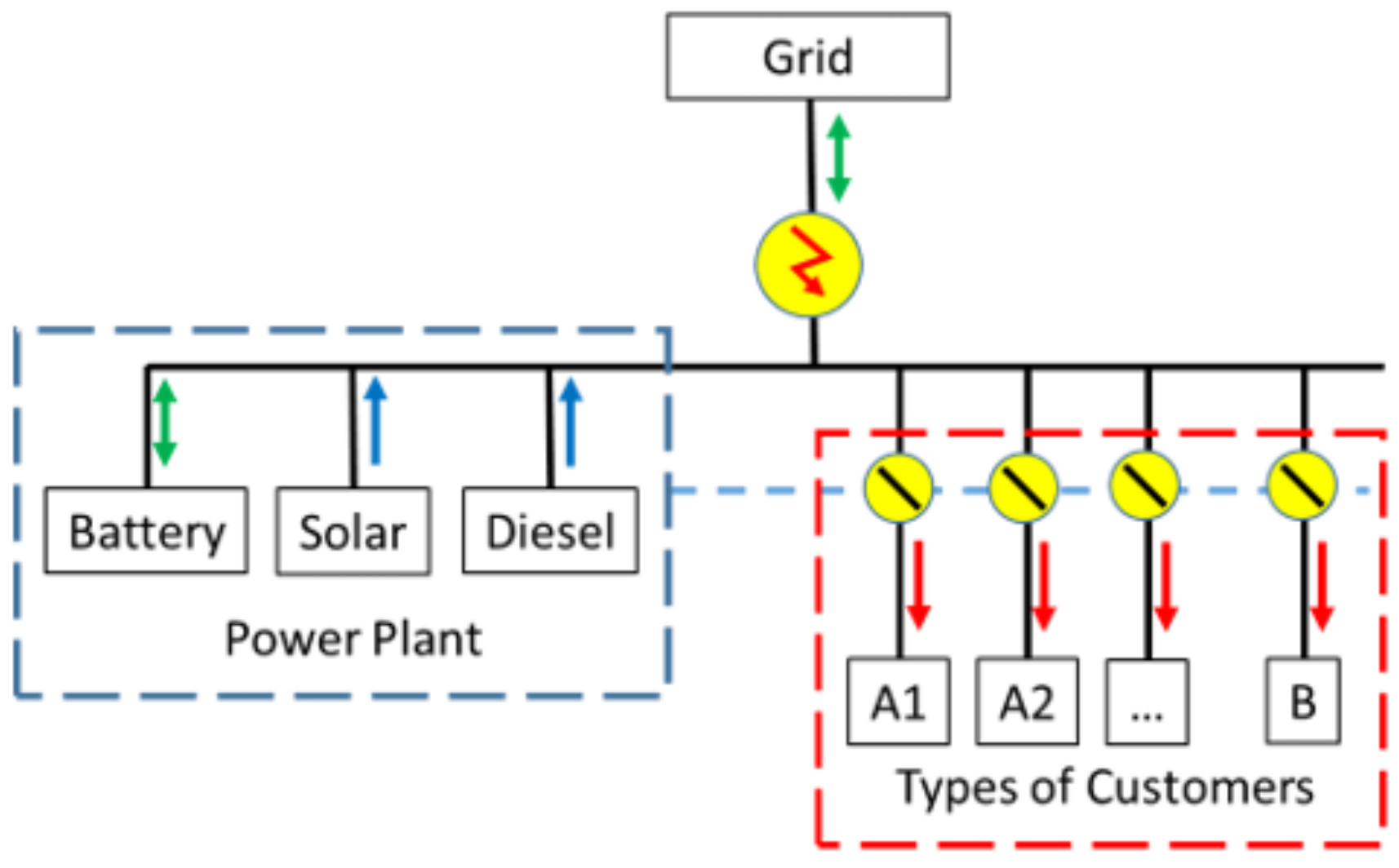
The UMG architecture is represented in Figure 1. It assumes a single connection point to the main grid, some local generation, storage assets and different types of demand. We assume a trading scheme exists, whereby electricity can be imported from the main grid to the mini-grid and vice versa. The MG can export or “feed-in energy” to the main grid at a Feed-in Tariff (FiT) or can import energy from the main grid at Bulk Purchasing Tariff (BPT). These energy exchanges are subject to variable spot prices. The spot prices, FiT and BPT, may be either real or artificial. In the first case, real transactions may happen between two different agents: the MG operator and the main grid company. In the second case, they are understood as price signals used for smooth coordination of multiple distributed resources. Real transactions could respond to a different (agreed) price or even not happen at all if the grid and the MG belong to the same agent. It is assumed that at each hour, the MG can either import or export from/to the main grid, but not both.
We assume that the main grid has an unreliable service. The reason for the main grid’s failures can be twofold: (a) the main grid has a capacity shortage or (b) transmission lines/poles fail. Under (a), the UMG can export electricity to the main grid (as a backup system) but not import, while under (b), the UMG cannot import nor export and operates on an isolated mode. The algorithm can handle both (a) and (b).
The UMG topological design shown in Figure 2 is adopted throughout the present work. It is a grid-connected hybrid AC-coupled micro-grid consisting of solar power photovoltaics (PV), a diesel generator (DG) and battery energy storage system (BESS) components. The PV array is connected via an inverter to the AC bus. The BESS can exchange energy bi-directionally with an alternate current (AC) bus via an inverter/rectifier. The loads, main grid and DG are directly connected to the AC bus. The efficiencies of the PV array and BESS are accounted for.
The model allows different types of consumer demands, with varying requirements of reliability that are represented in the market-logic model by different values for CNSE. The CNSE values assigned to demand types may be defined according to each context. In principle, they should exceed the actual retail tariff and include some pre-defined penalty for the lack of reliability. Alternatively, they might just be given ad hoc values so that the mini-grid behaves as expected. For instance, to prevent a particular customer type from being supplied by diesel.
It is further assumed that there are separate circuits and/or smart devices at consumers’ connection points, so that (a) different types of demand may be curtailed in different quantities, and (b) the aggregate demands of different customer types can be monitored separately. The effect is that a lack of supply does not cause a total black-out.
It is assumed that given forecasts for generating power from the PV array, load profiles for different customers, grid prices and main grid outages are accurate.
For simulation purposes, time steps have an hourly resolution; however, the model can be easily adapted to a minute or few minutes resolution for real-time (rolling horizon) management.
3. The UMG Market-Logic Operation Strategy
This section describes how the general market rules can be applied to the UMG unit commitment problem, considering the specific generation components of the mini-grid to define bids (prices and quantities) in a fictitious market and how to use this market model to find optimal dispatch decisions.
Traditionally, the UC and ED optimisation models were formulated for centralised vertically integrated structures, so the conventional scheduling problem minimises the total operating costs. However, with the gradual liberalisation of electricity markets, under a symmetric market pool scheme, generators bid to sell their power and independent system operators (ISOs) establish time-ahead and real-time operations. In this deregulated scheme, the UC’s objective changed to maximise social welfare, which is defined as the sum of producer and consumer surplus [46,47]. A symmetric market pool is based on a centralised virtual power market in which all power suppliers submit an offer bid a two-dimensional vector consisting of the lowest price per unit and maximum energy quantity that a supplier can offer, into the virtual pool. Correspondingly, the customers submit their demand bids, a pair made up of the demanded energy and the highest price that a customer is willing to pay per energy unit [45]. A market operator (MO) receives the virtual bids and offers; then, the MO carries out the optimisation task, seeking to maximise social welfare subject to an overall supply-demand balance constraint and respecting physical constraints. This process determines a market clearing price and a rate of production and consumption for each producer and consumer. In symmetric market pools, electricity is sold at a single price, the so-called market clearing price, which is subject to change every hour.
Although mini-grids are vertically integrated power systems, when connected to a central, possibly unreliable, main grid and with increased penetration of RES, their operation strategies are significantly modified. The traditional least-cost minimisation UC cannot optimally handle (with low computational effort): intermittent RES, frequent blackouts from the main-grid, demand-side management and supply for different types of customers with varying levels of reliability. This is why we propose a novel strategy for the operation of an UMG, based on the concept of the symmetric market pool [45].
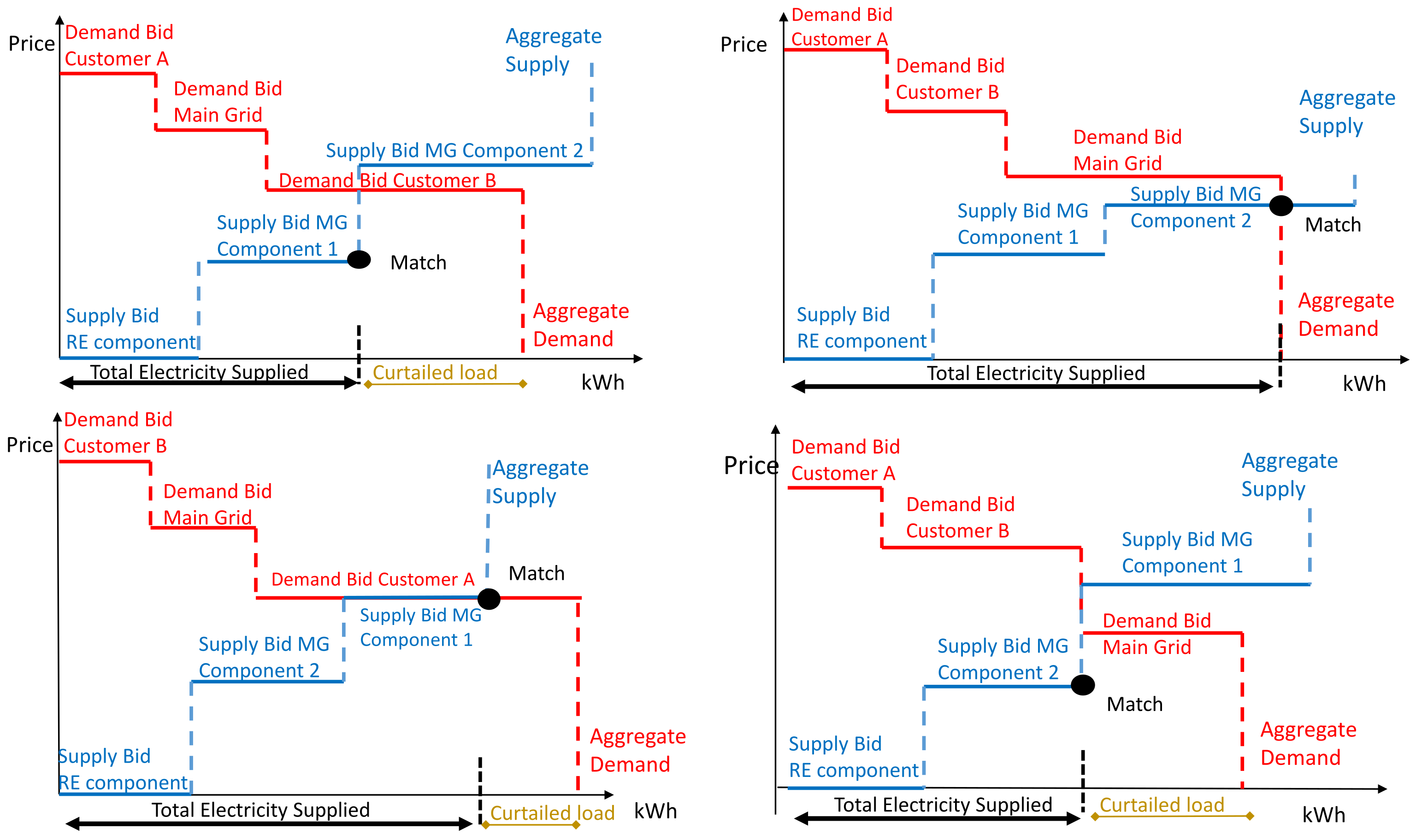
In the proposed approach, a fictitious market pool for the UMG is considered. Different UMG agents are assumed to “submit” hourly bids defined by price and quantity to the MG operator on a time-ahead basis. Supplier agents, such as solar PV and diesel generator (more generation technologies such as wind turbines or biomass could be added), participate by offering their hourly marginal generation costs and their capacity limits (subject to uncertainty in the PV or wind case). Examples of offer and demand bids under an UMG fictitious market pool are shown in Figure 3. The blue lines represent the offer bids of each mini-grid component, which comprise marginal costs (height in y-axis) and quantity of energy offered (length in x-axis). The blue lines are arranged in an ascending order to form an aggregate supply curve, while the red lines represent the demand bids of different types of customers and main grid with their predetermined tariff levels and CNSE (height in y-axis) and variable loads (length in x-axis). The demand bids are ordered by the CNSE or tariff in descending order (those with premium supply contracts are assigned a higher priority in receiving electricity). Following the market pool model, the demand and offer bids form the aggregate demand and supply step curves. The intersection point (match) determines a market clearing price and a rate of production and consumption for each producer and consumer. However, in our fictitious UMG market model, the hourly market clearing price (height of intersection point in y-axis) is ignored, since tariffs are set a priori and MG energy is not necessarily sold at a single price. We focus our attention only on the UMG’s quantity of dispatched energy and the amount of curtailed energy for certain types of customers (lengths in x-axes). As shown in the four examples of Figure 3, the total quantity of energy supplied and the smart curtailment are set by the highest accepted UMG component to offer.
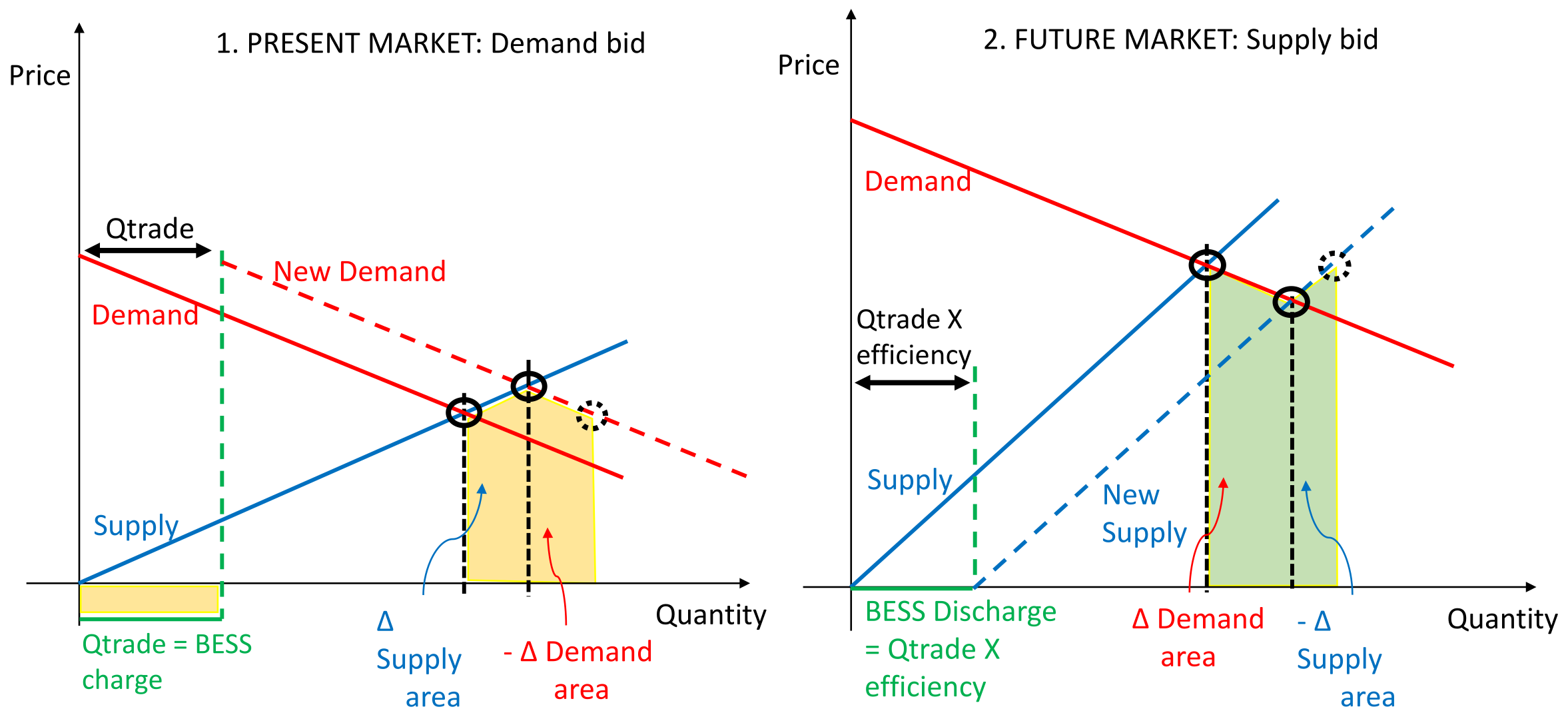
Furthermore, we define generation shifting as postponing supply of electricity from one time period to another. In the UMG operation problem, the prosumers—BESS and main-grid—are special agents in the market pool, since they can control generation and load shifting. BESS can buy (charge) or sell (discharge) energy; their actions are not modelled as bids but as market interventions that cause displacements of the demand or supply curves. Quantities are limited by maximum power and the state of charge (SOC). BESS prices are defined to be a very small positive quantity strictly greater than the cost of PV. Batteries are special since they are the only agents able to consider the future: they reduce welfare in one hourly market to increase welfare in a future hourly market. They intervene in the markets with absolute authority for the general good.
Figure 4 depicts an example of BESS’ demand (charge) and supply (discharge) actions in a present and future market. Markets are matched without battery. The present market has operative grid, no solar power and high grid prices. Two alternative future markets are shown. Demand actions cause welfare loss (area in yellow), while supply actions increase welfare (area in green). The total increment of welfare is positive, as expected when buying at a low price and selling at a high price.
4. Mathematical Formulation: Undergrid Mini-Grid’s Market-Driven Unit Commitment
Redefining the UC problem for mini-grids in a market-logic approach, as described above, involves three modifications compared to the formulation in a vertically integrated environment: (1) changing the objective function from cost minimisation to social welfare maximisation; (2) the demand to be served includes multiple types of customers with different reliability requirements and contracts; (3) adding slack variables to the power balance equation characterising the NSE corresponding to the number of types of loads; (4) penalizing the cost of NSE in the objective function by previously stipulated price contracts. The mathematical formulation results in a deterministic mixed-integer linear program. For this model, we assume that the design and the size of the components are fixed and given exogenously. It is also required to input forecasts for: maximum solar generation , spot grid prices , demand profiles for different customers , and main grid’s outages data .
4.1. Objective Function
The aim of the optimisation problem, as explained in the previous section, is to maximise the hourly social welfare, i.e., consumer plus producer surplus such that power is balanced at all periods of time. Therefore, the objective function is given by:
where are the number of customers—Type A and Type B; are the load forecasting of customers—Type A and Type B at time t; are the retail tariffs for customers—Type A and Type B—at time t; are the decision variables representing the amount of not served energy for customers—Type A and Type B at time t; and are the predetermined costs for not serving energy to customers—Type A and Type B. is the FiT for exporting energy to the grid, and is the electricity exported to the Main Grid at time t. The fuel cost function of the diesel generator can be expressed by a linear Equation [48,49], where is the marginal cost of diesel , b is the intercept coefficient of the fuel curve in , m is the slope coefficient of the fuel curve , is the rated capacity of the DG, is the power output of the DG at time t, is a binary variable that represents the on and off status of the DG, is a binary variable of the operating state of the DG, and is the startup cost of the DG. Lastly, is the marginal cost of energy from PV, is the electricity output of PV at time interval t; is the BPT for importing energy from the main grid at time t, and is the electricity imported from the main grid at time interval t. The objective function is depicted in Figure 5. On the left the demand bids are defined by the customer tariffs with no CNSE (height in the y-axis) and loads (in the x-axis).
The total welfare (area in yellow) is the area under the demand curve minus the area under the supply curve. On the right, the demand bids are defined by tariff levels and CNSE, as formulated in (1). It is shown how reducing the supplied energy to customer A reduces the total welfare area at time t quite significantly since is high. Curtailing a fraction of load B, which could be served with solar energy, and instead charging the BESS, also reduces the welfare at time t, but it might be optimal to increase welfare at another future time t.
4.2. Constraints
1. First Kirchhoff Law or Power Balance:
where are the number of customers—Type A and Type B; are the load forecastings of customers—Type A and Type B at time t; is the electricity exported to the Main Grid at time t; is the amount of battery charge at time interval t; and are the efficiency parameter when charging the battery and the efficiency of the rectifier, respectively; is the efficiency of PV Inverter and is the electricity output of PV at time t; is the power output of the DG at time t; represents battery discharge at time t; and are the efficiency parameter when discharging the BESS and the average efficiency of the BESS-Inverter; is the electricity imported from the main grid at time t; and are two slack variables representing the amount of not served energy for customer-Type A and customers-Type B, respectively.
2. Definition of cost of not-served energy per customer in each period t:
where are the MG penalties for not serving Type-A and Type-B customers, respectively. These penalties are defined by the cost of not serving electricity per customer type minus the given tariff per customer type .
3. PV generation limits in each period t:
The daily PV time-series generation, denoted by , is constrained by the forecasting of maximum PV power production, denoted by . Furthermore, the PV inverter converts the variable direct current (DC) output of a PV into a utility frequency alternating current (AC), which is fed into the AC Bus. The efficiency of the PV inverter, denoted by , indicates how much DC power is converted to AC power.
4. Dynamics of the battery:
The BESS performance is represented, like in [50], in terms of the instantaneous state of charge , which is a function of the SOC in the previous period of time , the self-discharge rate , and the amount of BESS charge at time t minus the amount of BESS discharge at time t. Moreover, the state of charge has a lower limit given by the minimum state of scharge and an upper limit given by the maximum state of charge .
5. Storage battery maximal generation in each period:
The amount of BESS’ discharge has as upper bound the maximal BESS discharge limit , multiplied by the binary variable representing the discharging state of the BESS.
6. Storage battery maximal consumption in each period:
The amount of BESS’ charge has as upper bound the minimal BESS charge limit , multiplied by the binary variable representing the charging state of the BESS.
7. The battery cannot charge and discharge at the same time t:
where the binary variables represent the discharging and charging state of the BESS, respectively.
8. Diesel generation upper and lower limit in each period t:
9. By definition, and are closely related to . The relation between these variables is given by:
Here, is the binary variable representing when the DG starts to run at time t, while is the binary variable representing when the DG is stopped at time t. As is a binary variable representing the on and off state of the DG, if the on/off status changes between time interval t and , then either or . Else everything is equal to zero.
10. As the diesel generator is a thermal energy source, we provide a more descriptive and general model as in [51]. When the diesel generator starts to run, it has a minimum duration period to stop generating power:
where is the minimum running time of the DG.
11. On the other hand, once the diesel generator is stopped, it can only run after a resting time.
where is the minimum resting time of the DG.
12. The quantity of electricity exported to the grid, denoted by , is less than or equal to the maximal transmission capacity, denoted by .
since one can only import or export at each time period t, the upper limit is multiplied by the binary variable , representing the export to the main grid state at time t.
13. The quantity of electricity imported from the grid, denoted by , is lower than the maximal transmission capacity .
where is a binary variable representing the outage or availability of the main grid. One cannot import from the grid at the periods when it fails ().
14. The charging and discharging limits given by the Nominal Power of the BESS Inverter-Rectifier, denoted by :
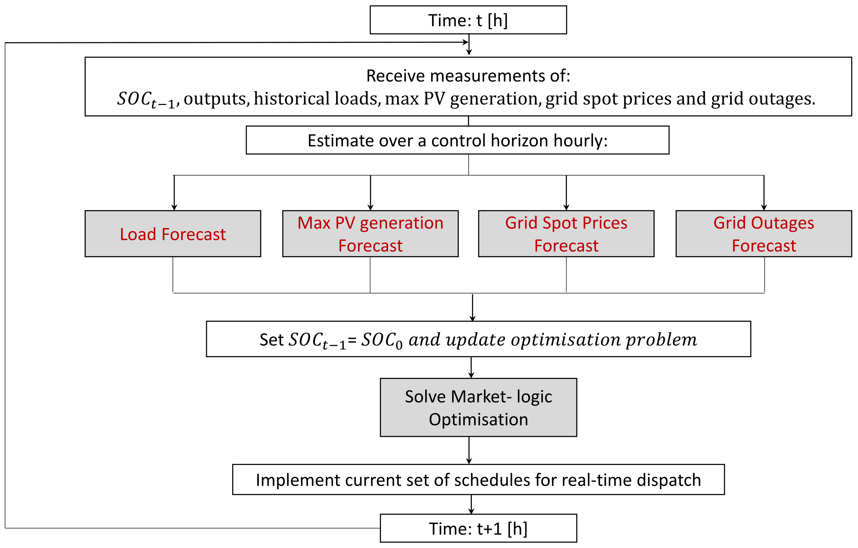
The MPC technique applied in the market-logic UMG scheduling is presented in Figure 6. The scheduling repeats every hour. At the execution of the hour t, the operator receives measurements from BESS and historical data of key input uncertain variables. For a chosen time horizon, i.e., next 48 h, forecasts of key input variables are figured out. Then, the forecasts are formulated into the UC optimisation model and updates the optimisation model with new feedback. Next, the optimal commitment and dispatch is computed for all MG components under the given time horizon. Then, the computed outputs associated with the current time-steps on the physical MG operation are implmented. Finally, one moves one time horizon ahead for the next period, updates forecasts based on newly available measurements and repeats the real-time optimisation procedure. The repeated optimisation procedure provides closed-loop feedback and enables the MPC to counteract key uncertainties present in the MG operation.
5. Case Study
This section presents computational results illustrating the proposed operation strategy. Accordingly, six scenarios are analysed including three grid modes: 100% reliable grid, unreliable grid and isolated MG; and two solar resource availability modes: dry and rainy season. For the simulations, a weekly horizon was considered with hourly time-steps. The MILP model has been implemented on the GAMS platform [52] and solved with CPLEX on an Intel(R) Core(TM) i5-8265U CPU, and each simulation was completed in 4.2 s.
5.1. Description of Inputs
To verify the advantages of the UC method, we analyse a case study in Nigeria, but the model can be adapted to any undergrid mini-grid. A hybrid PV-battery-diesel UMG will be installed in 2022 at Kare, Kebbi State of Nigeria. Herein, we contextualize the input parameters. It is assumed for simplicity that there are two types of customers: customers A, with a high reliability contract and therefore higher retail tariff, and customers B, with a lower tariff-level, which can be curtailed ( = 0.5 $/kWh, = 0.2 $/kWh) and prevented from being supplied by diesel. In Nigeria, the Regulation for Mini-grids released in 2017 by the Nigerian Energy Regulation Commission (NERC), stipulates that grid-connected MG operators can set a cost-reflective tariff for different types of customers, but it is fixed on a yearly basis. This is why we assume time-independent retail prices for two differentiated customers. Table A1 in Appendix A summarises further parameter values used in the case study.
Regarding time series, historical solar irradiation data for the provided GPS coordinates was computed from NASA database [53] and used for the given PV configuration (see Table A1) to model the maximum PV output at each hour t. For the unreliable main grid scenario, a daily average interruption frequency of Int/day with an average interruption duration of h is assumed. Based on the given input, pseudo-random outages were generated, and unscheduled grid outages were simulated and are shown on the respective scenario results. Furthermore, since there is still no regulation regarding the costs and pricing structure for importing and exporting from/to the main grid, for modeling purposes, we assumed changing profiles as shown in Figure A2 in Appendix A. Lastly, the cumulative load profiles for customer group A and customer group B assume an average daily electricity consumption of 146 kWh for customer A and 82 kWh for customer B.
5.2. Results and Discussion
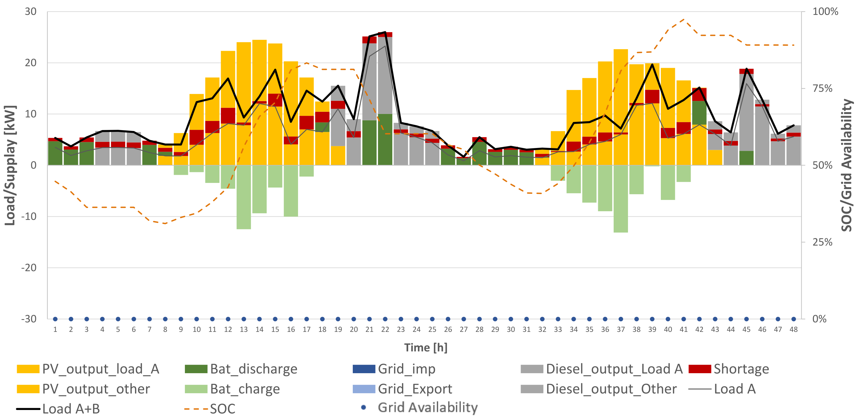
The six simulation results of the case study under our market-logic approach are shown in the following figures. Figure 7 and Figure 8 show the dry-season results for both a 100% reliable main grid and an unreliable main grid. Figure 9 and Figure 10 display the rainy-season results for the same two main grid scenarios. Lastly, Figure 11 and Figure 12 show the isolated mini-grid cases, comparing dry and rainy seasons.
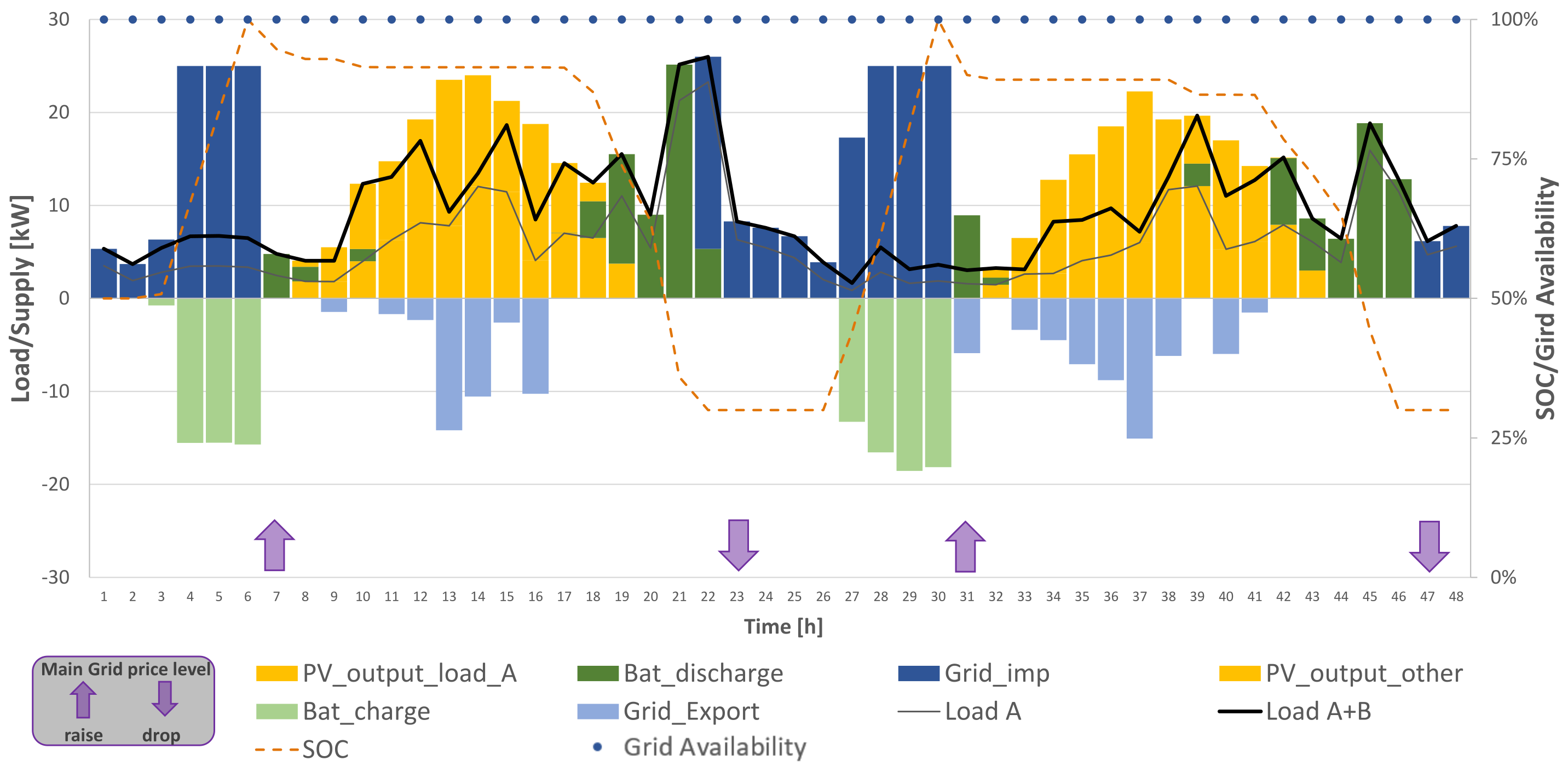
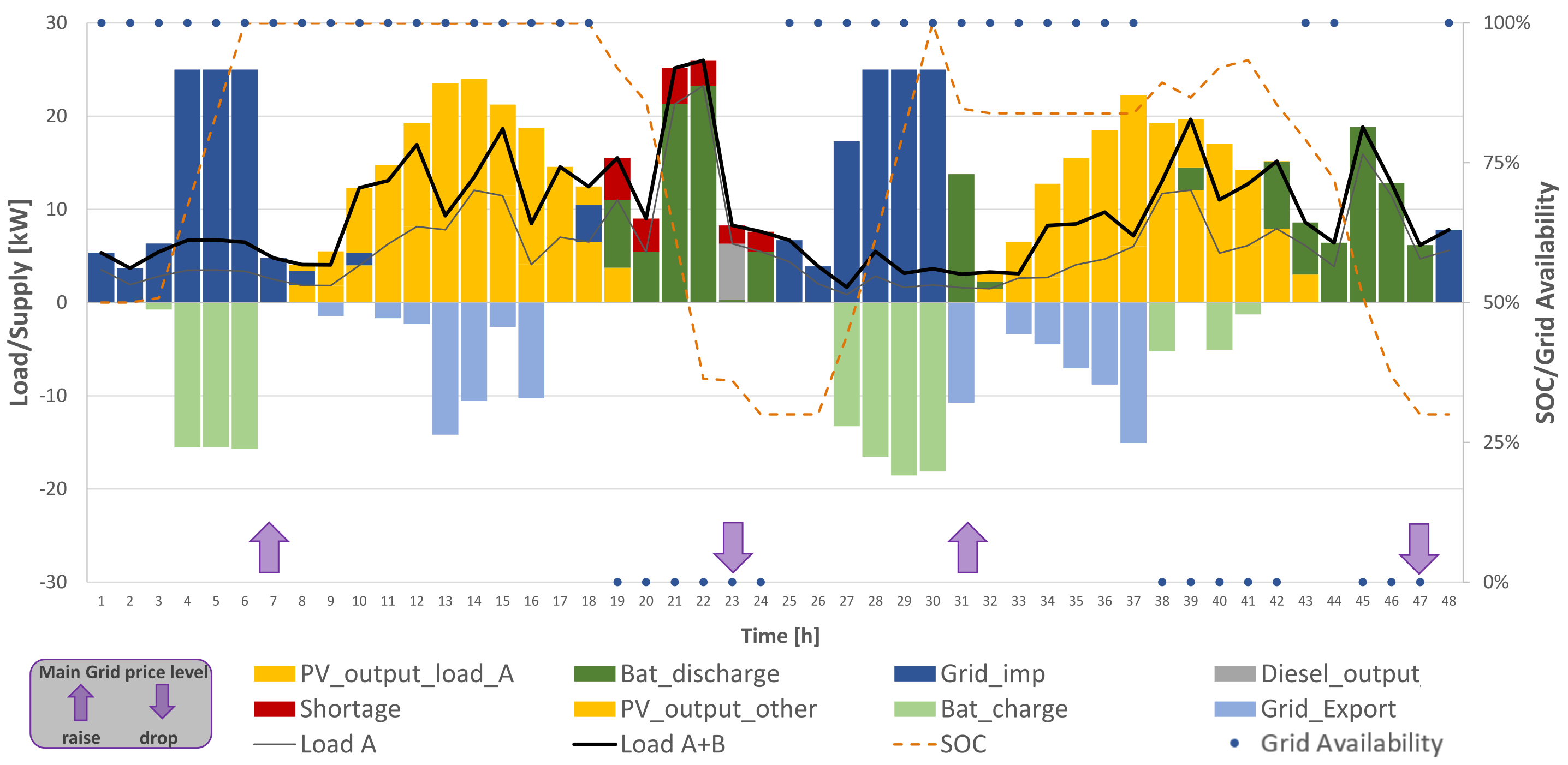
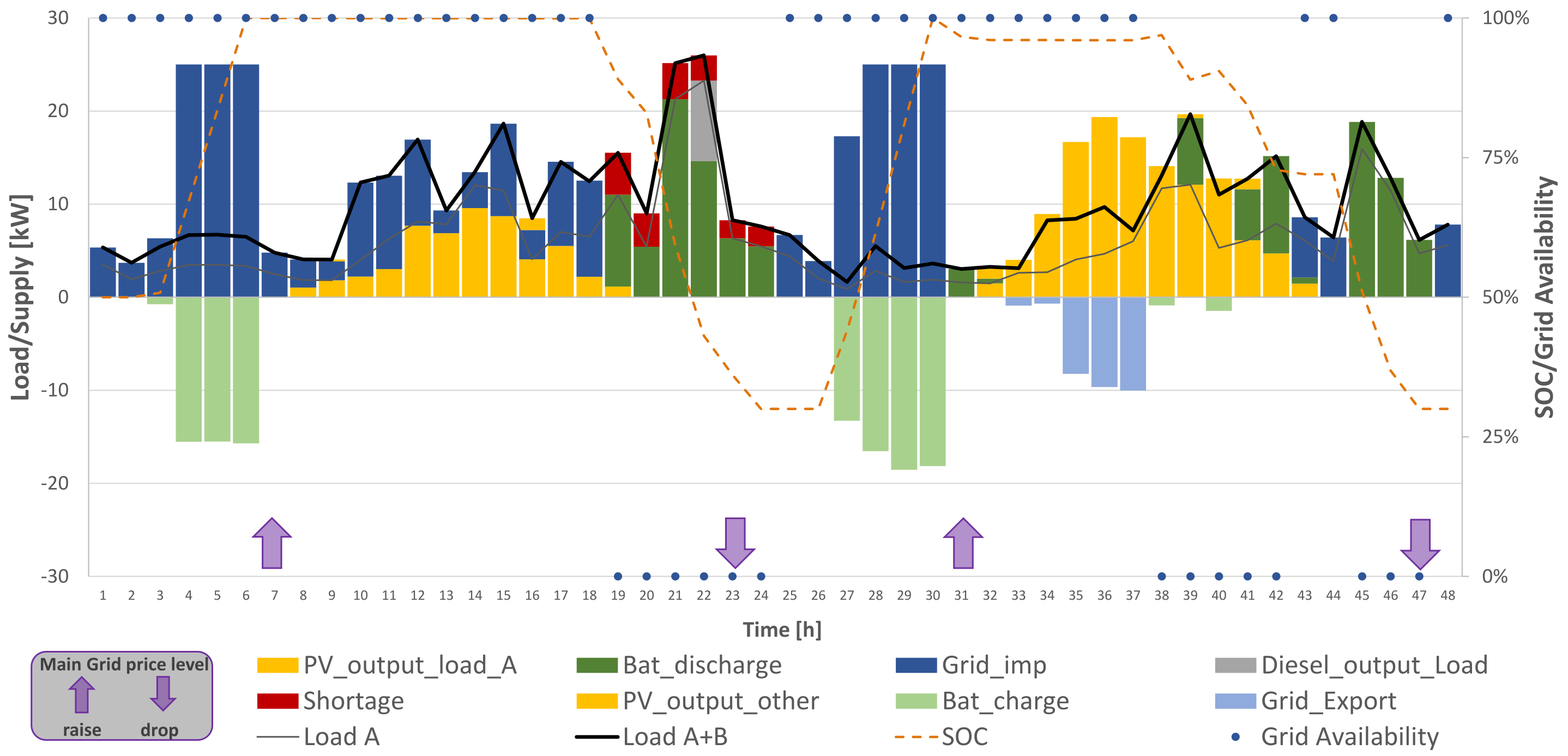
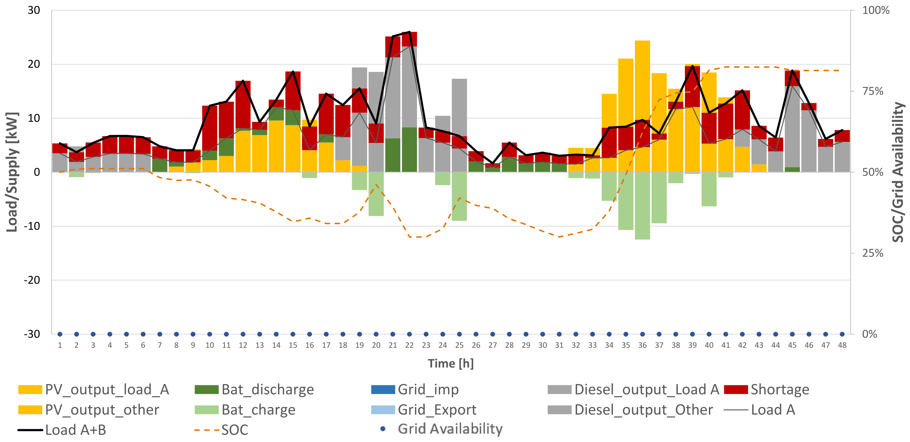
To ease visualisation, we portrayed only the first 48 h of the one-week dispatch. The figures depict in the positive region the cumulative load of customers and power supply (generation, battery discharge and grid import). Battery charge and export of energy to the grid (special types of demand) are represented in the negative region in order to identify clearly what use is made of the generation or import surplus. Figures also show the evolution of battery SOC over time (orange segments, scale at the right side), the availability of the grid (blue dots, scale at the right side), and the changes in the grid energy prices (up or down arrows). The reliability level, energy not served, costs and welfare for all scenarios of our case study are listed in Table 1 and Table 2.
Figure 7 shows how the battery is mainly used to trade energy with the main grid: it is charged in the early hours of the morning, at low price, and discharged in the afternoon-evening hours (at high price). The solar surplus is sold to the grid at high price. Furthermore, this scenario reveals that the market-logic approach integrates price signals for generation shifts. At low BPT levels, the main grid energy is used to charge the battery (3–6 h and 27–30 h), and the MG sells part of that energy to the main grid in the next period of higher FIT-level (31 h).
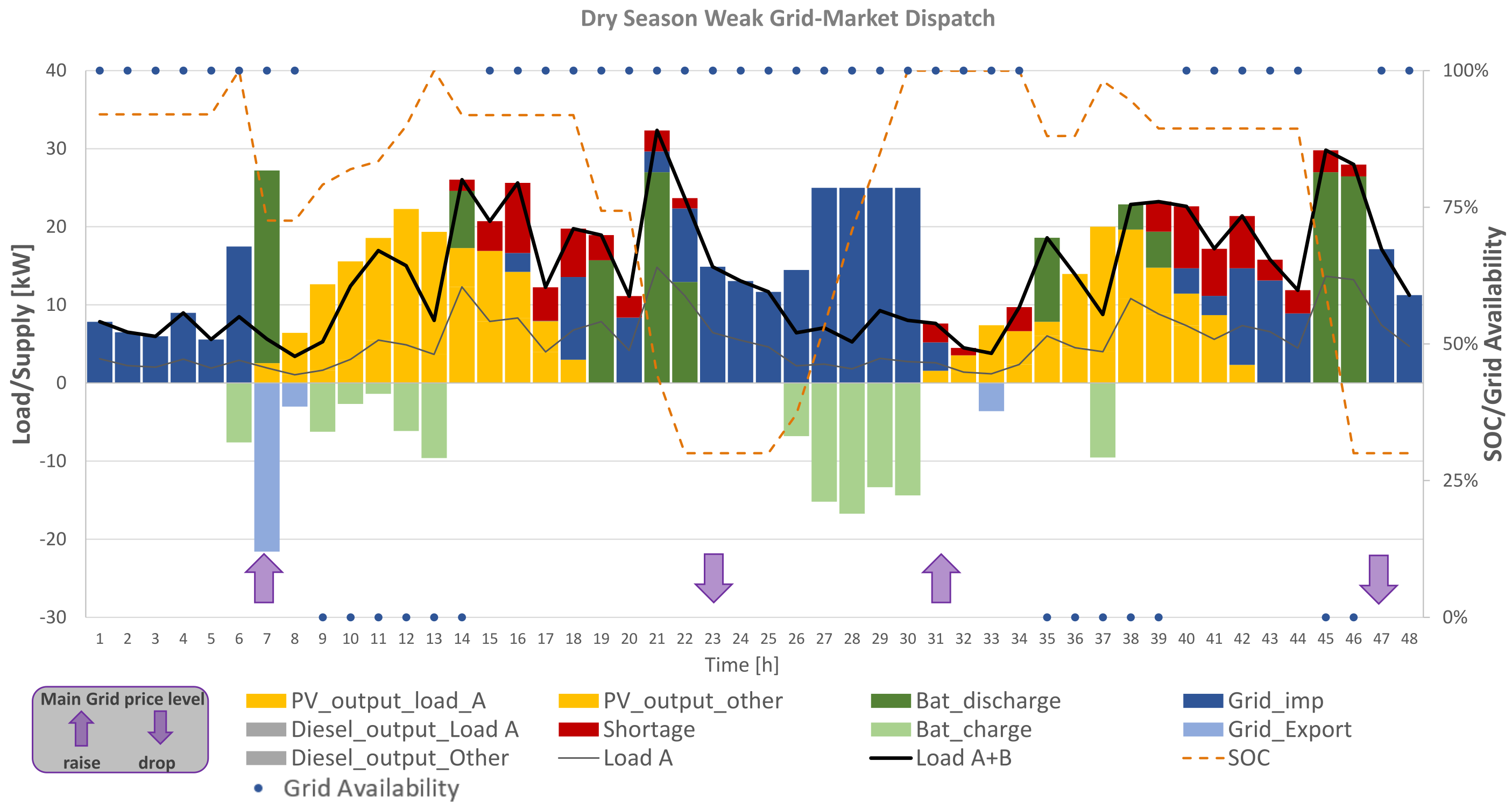
Figure 8 shows behavioural changes due to failures. Here, one can appreciate that the market-logic dispatch follows grid price signals to decide on smart curtailment and load shift. In hours when there is sun or the main grid is available at low BPT, all types of customers are served. Whereas in hours when there is sun, the main grid is available and the FiT-level is relatively high, energy is sold to the main grid even if the SOC is still below 100% (see 33–41 h).
Moreover, the long failure at the end of the first day causes the use of diesel, and some curtailments for Type-B customers. This is because the battery is not big enough to cover that demand, and Type-B customers are never supplied with diesel due to the selected input cost values. In the second day, the battery management is perfectly adapted to future failures and less solar production. Of course, this behaviour is only feasible if predictions for uncertain time series are accurate. Note the possibility of programmed outages in areas with generation capacity shortages; this shows that the reduction of uncertainty may have a dramatic effect in reliability and costs.
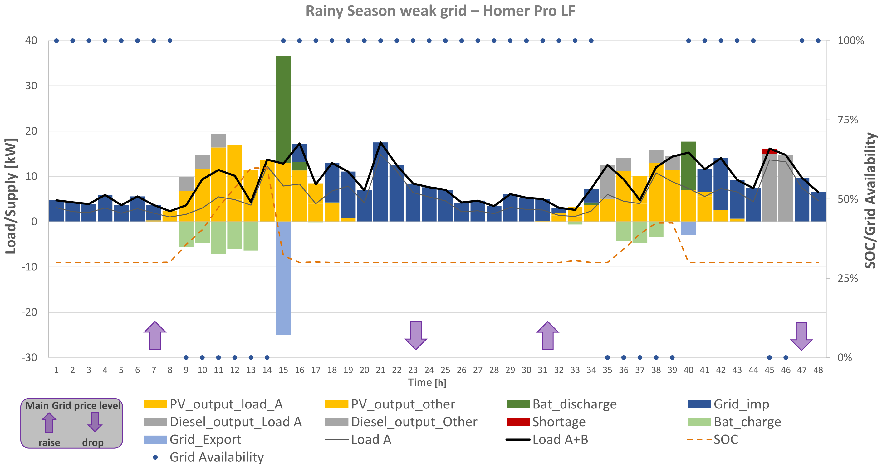
Figure 9 and Figure 10 portray the same cases as in Figure 7 and Figure 8, but with less solar production (rainy season). Uncertainty of the main grid service is critical. In the rainy season, a full grid the total demand is served, while in the unreliable rainy season grid, at night-time, when the grid is not available, load B is not served. Battery capacity is only used to serve load A. When the grid is unreliable, the optimal dispatch saves the battery discharge for the times when the grid is available and serves a total load with sun and grid import (Figure 10 8: 18 h). On the contrary, in rainy season, full grid the battery is discharged to serve customer B. Another important aspect is that the battery is more often maintained at full charge under an unreliable grid scenario and rapidly discharged after full charge in a 100% reliable grid. Depending on the battery type (lead acid or Li-Ion), this could have positive or negative influence on the battery lifetime.
Figure 8 and Figure 10 show that changes in solar availability have no effect in the overall management of the UMG. The main difference is in the trading with the grid: the lack of solar production makes the system import more energy from the grid and export less.
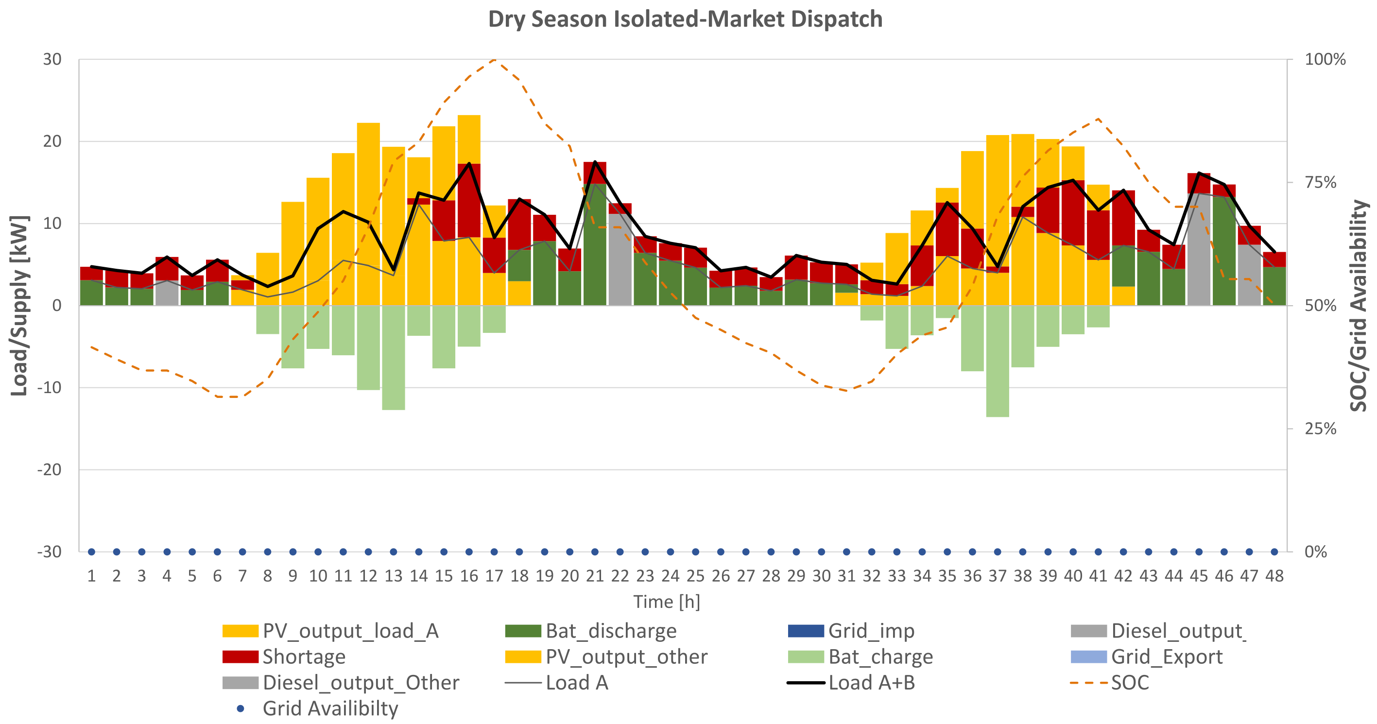
Figure 11 and Figure 12 show the simulation cases for an isolated mini-grid. The battery is used, when possible, to store solar surplus and save diesel usage at night. Note that even in hours of solar surplus, Type-B customers can be curtailed, charging the battery instead of being supplied. This is because of the need for battery energy at night, both to save diesel and to supply Type-A customers in full.
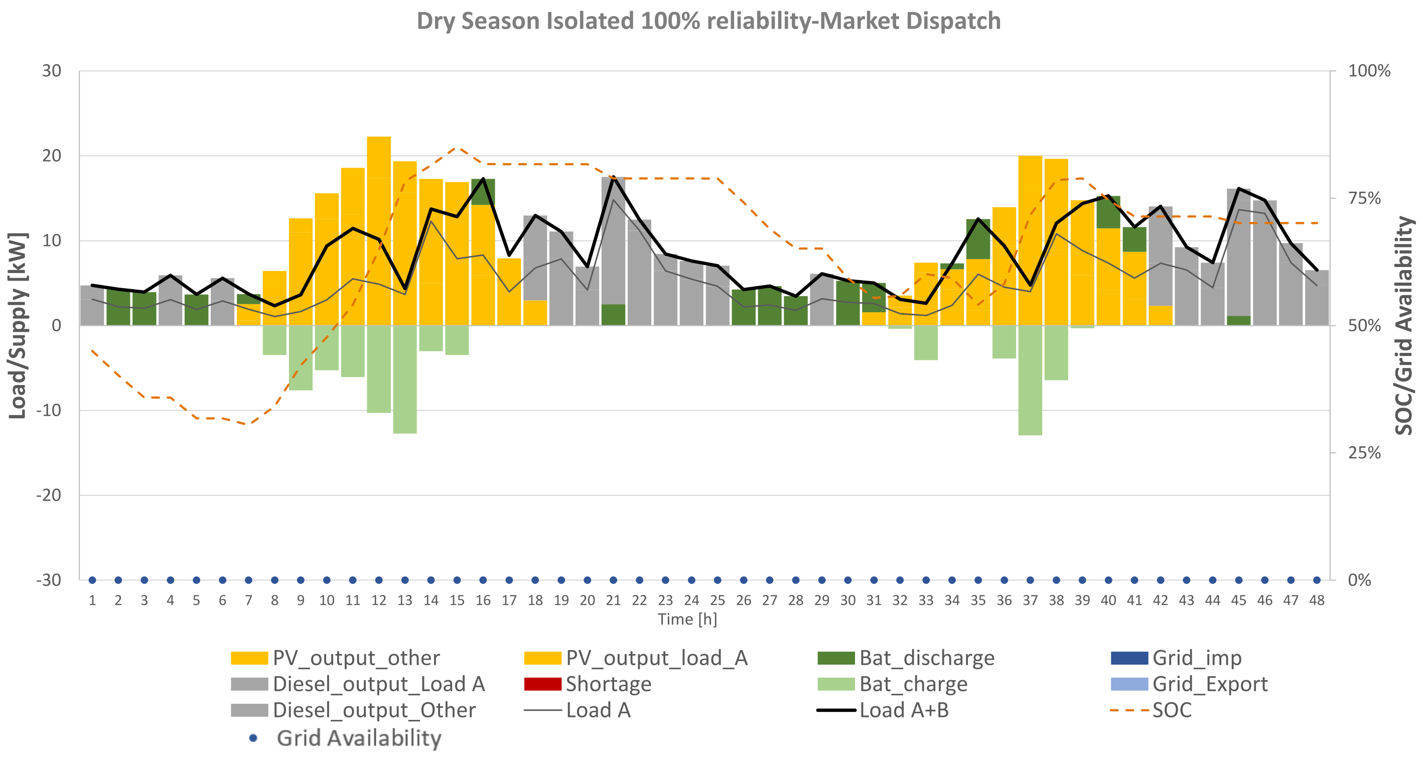
Figure 9 and Figure 12 portray how, under the market logic, customers B are curtailed and energy is rather stored in the BESS for later supply of load A. Load B is only served on a reliable basis in the scenario with 100% grid availability, since the assumed retail tariff for customers B does not cover operational costs of the diesel generator. In Table 1, the reliability of load B stands out from off-grid dry season and off-grid rainy season. Although these are the optimal solutions given the price signals, it might be politically required to add a minimum reliability constraint for each customer type. For illustrative purposes, Figure A3 in the Appendix A shows the optimal dispatch under dry season, where hourly supply for load B is additionally constrained by a reliability level.
All these results also provide insights into the optimal sizing problem and the value of forecasting for different sources of uncertainty. It can be seen that the dispatch of the rainy season full grid and dry season full grid are very similar. The slight difference is that in rainy season more energy is imported from the grid, so the operation costs are slightly higher. Thus, interestingly, solar energy is not a critical uncertainty for an UMG; moreover, it is rather easy to forecast it in the short term. In contrast, uncertainty of the main grid’s outages is very relevant, and they are difficult to predict in general (see Table 2 comparing the results of rainy season with different main grid availability levels).
6. Comparison
In this section, typical heuristic system operation schemes such as LF and CC used by HOMER Pro for the UMG system dispatch optimisation are compared with the proposed predictive deterministic strategy of the market logic. We also compared the HOMER Pro Predictive controller (PS) algorithm to our proposed market-logic predictive dispatch to allow for better direct comparison. For the simulations presented here, a two-day horizon was considered.
6.1. Description of Inputs
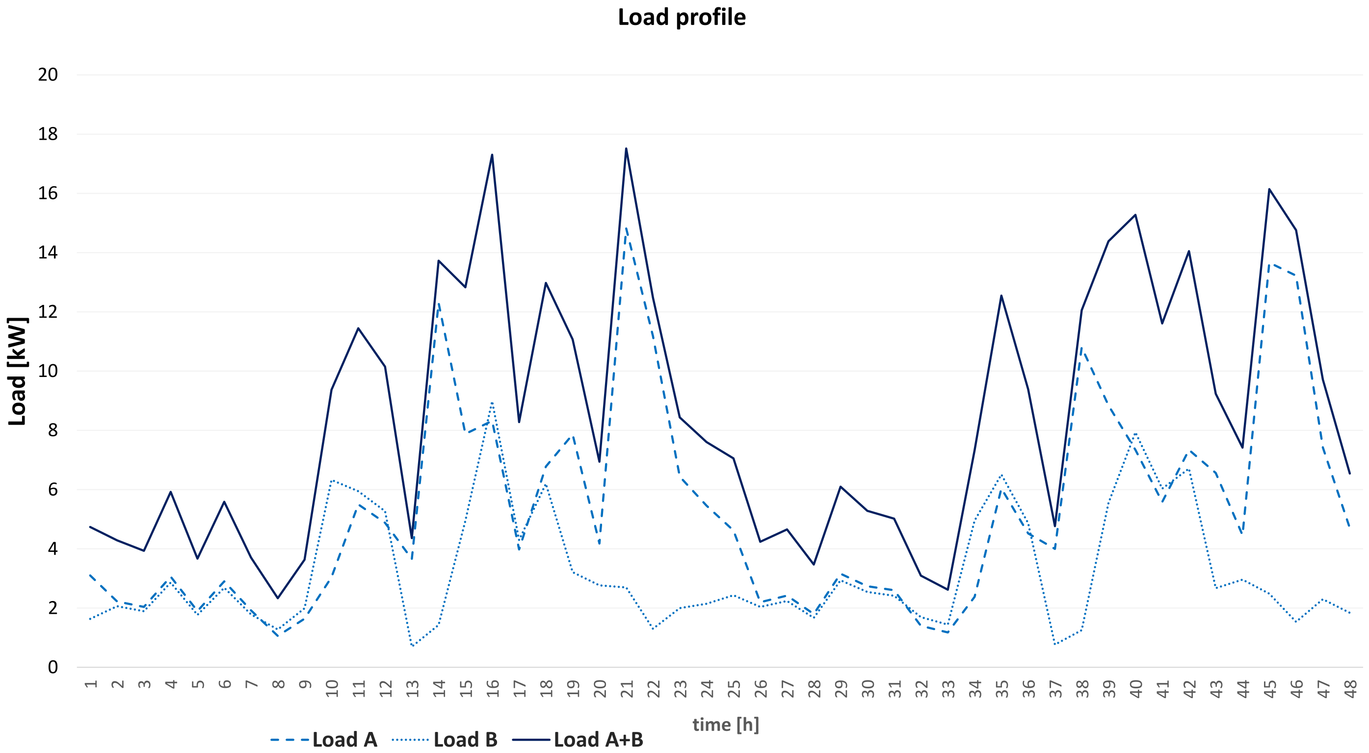
The input data for the UMG system design and parameters have been fixed in HOMER Pro according to a previous section (see Table A1 in the Appendix A). Since HOMER minimises costs it does not take into account tariffs nor CNSE input data. We have extracted the resulting dispatch decisions from the result export file generated by HOMER Pro. For the sake of comparison, we have input different time series as in the previous section. We assume here 48 h foresight for all time series. Load profiles A and B, maximum PV Output, grid availability and spot grid prices can be found in Figure A4–Figure A6 in the Appendix A.
6.2. Discussion
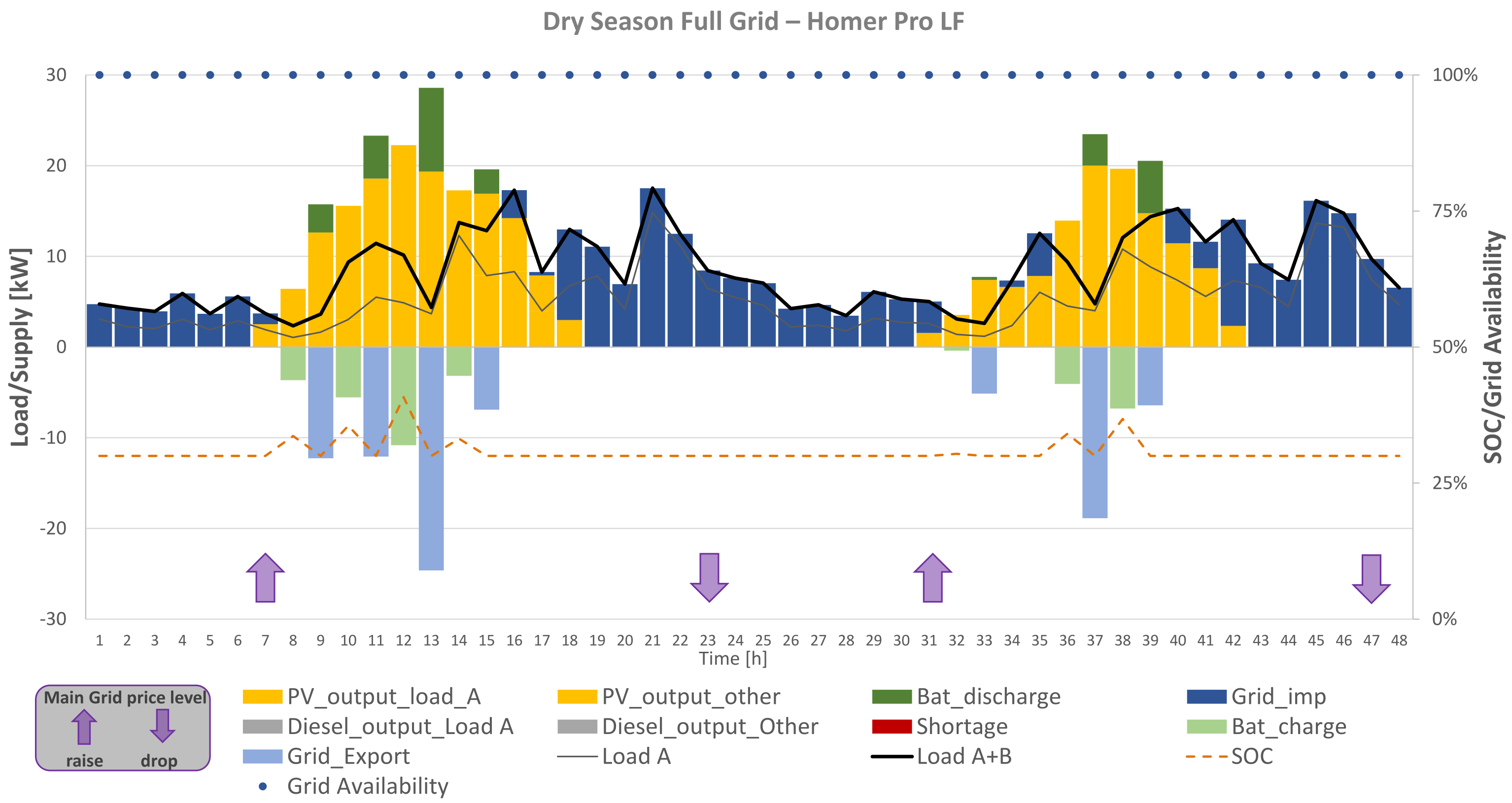
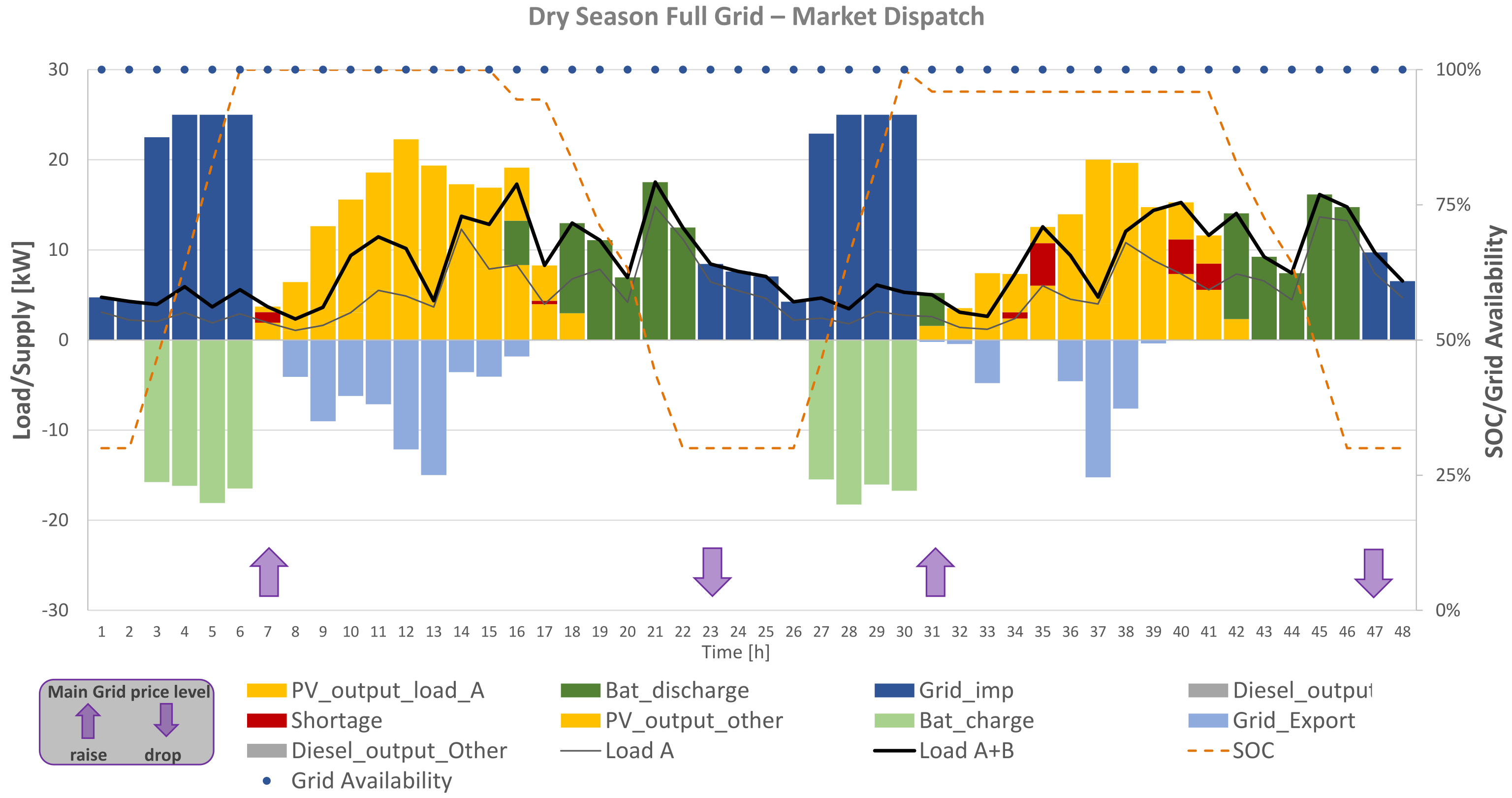
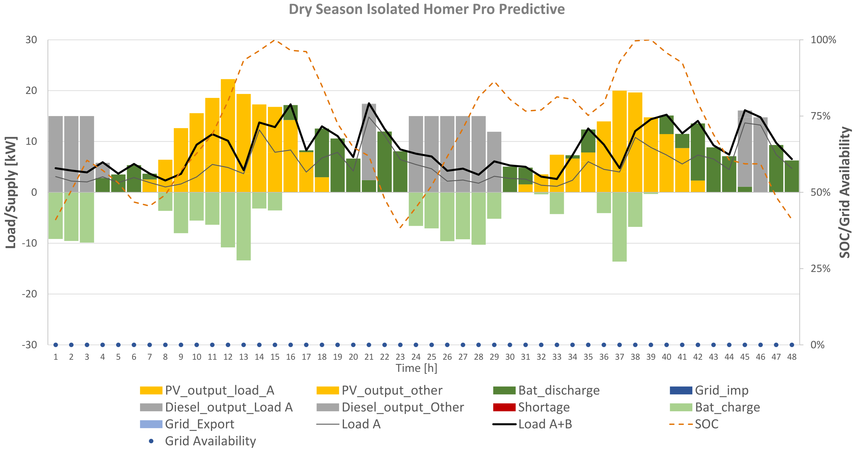
We present four comparisons between the market-logic dispatch and HOMER Pro’s dispatch models. Figure 13 and Figure 14 show the UC results during the dry season with a 100% reliable main grid for both the the HOMER Pro LF strategy and the market-logic dispatch. Figure 15 and Figure 16 show the UC results during the rainy season with an unreliable main grid for both the HOMER Pro LF strategy and the market logic dispatch. Figure 17 and Figure 18 show the UC results during the dry season with an unreliable main grid for both the market logic dispatch and the HOMER Pro CC strategy. For the latter, we have doubled the load A to portray the use of diesel genset under the CC strategy. Lastly, Figure 19, Figure 20 and Figure 21 show the UC results for an isolated MG during dry season for both predictive approaches: the market-logic model and HOMER’s PS.
Figure 13 shows that the single-time-step-based heuristic method of the Homer LF strategy leads to a sub-optimal battery usage compared to the market dispatch strategy in Figure 14. The SOC level under the HOMER LF approach is mainly kept low. During hours 8–15, the battery is charged with excess solar energy and sold in the next time step iteratively. This strategy leads to an empty battery at night time (17 h), and the UMG is obliged to purchase energy from the grid, although hours 17–23 have a high price zone. Instead, the market-logic model uses the varying grid import and export prices of the fully available grid. It charges the battery at low tariffs to supply loads A and B and generates additional welfare by trading with the grid. The assumed tariff and cost structure make it disadvantageous to supply load B, and solar excess is rather sold directly to the main grid at periods high sale prices. Depending on real regulatory constraints and market conditions, it is likely that these assumptions might not apply, and extra constraints would be applied accordingly. From Table 3. we see that the market-logic dispatch has lower OPEX and higher total welfare.
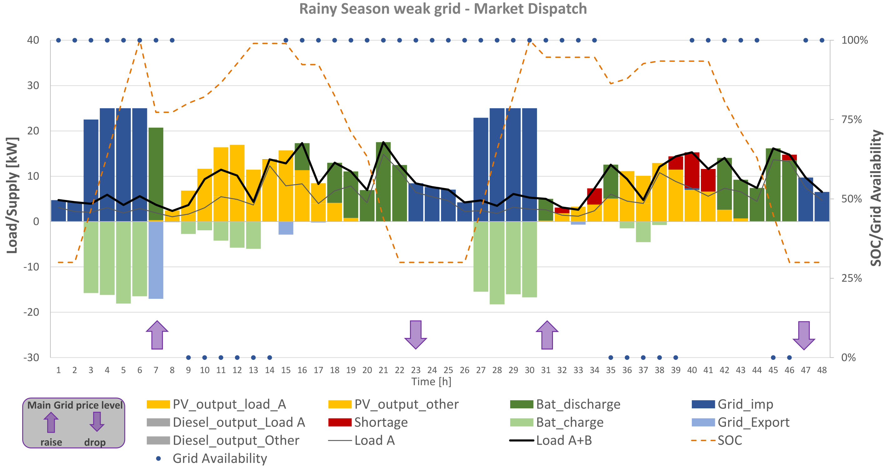
Figure 15 shows that the heuristic LF dispatch strategy does not make proper use of the battery, since the SOC level does not reach its maximum. In consequence, it has a capacity shortage of hour 45. Furthermore, the LF strategy leads to a sub-optimal economic decision by exporting to the main grid renewable energy from the battery in one time-step (hour 15) with favourable prices but is obliged to purchase high tariff energy from the grid in the future (hours 18–22).
Figure 16 shows a more accurate use of the battery when trading with the main grid. It charges the battery until its maximum SOC level when the grid spot prices are low and imports to the main grid by discharging to the minimum SOC level when prices are high. From the graphs and Table 4 , we see that the LF strategy leads to additional diesel genset usage (above 50 kWh), which is more than what the market-logic dispatch curtails to load B (22 kWh). Furthermore, the operating costs are lower in the market-logic.
Figure 17 shows that the CC strategy does not involve trading with the grid to make use of the profit margin resulting from the BPT and FiT variation. However, under the market dispatch strategy shown in Figure 18, trading with the main grid is done to increase the welfare (i.e., time-steps 6 and 7). Due to the low-tariff incentives for serving load B, under the market approach, load B is regularly curtailed and only served with low tariff grid energy and direct solar energy. In contrast, the CC time-step-based approach uses the energy from the grid for night loads, thereby allowing for an almost fully charged battery in the morning, which does not allow for storing the excess solar energy. This dispatch harms the renewable fraction and leads to higher operational costs (see Table 5 for more details).
Figure 19 and Table 6 show that the smart curtailment allows for a significant welfare increase compared to the predictive dispatch by HOMER Pro. This is because no high-cost energy source (diesel) is used to cover low-tariff load B. Under the market logic, load B is served during day-time under the condition that the battery can still be fully charged before dusk to serve Load A during night-time.
In order to allow for a direct more equal comparison of the dispatch strategies by the HOMER Pro PS and the market-logic approach, we performed an additional simulation, shown in Figure 21, of the market-logic approach assuming a regulatory, not market-driven, constraint of 100% reliability for Loads A and B. The comparison still shows the cost advantage of our proposed model against the predictive dispatch approach provided by HOMER PS in Figure 20 (see also Table 6). Although under the market-logic strategy, the DG runs in a less optimal operation mode than in HOMER PS, the market dispatch avoids that the DG charges the battery. The market dispatch makes the more adequate choice to only charge the battery with solar as the DG is always available as back-up. In fact, the comparison with HOMER PS could be done for the isolated scenario as HOMER’s predictive strategy does not allow to model a grid-connected MG. The latter shows a further advantage of our proposed model, which allows for the consideration of isolated MG, UMG and a reliable and unreliable grid connection.
7. Conclusions and Further Developments
This study has presented, implemented and tested a novel dispatch strategy for UMGs, which can be used in the development of smart energy management systems and as an essential constituent in the design of UMGs. The strategy is based on combining straight market pricing rules in the hourly short-term dimension with maximisation of the hourly social welfare over the multi-day relevant decision-making period. The mathematical formulation results in a deterministic MILP. It is assumed that key input uncertain parameters are well predicted in advance. It is therefore a predictive algorithm, whose conclusions can provide useful insights but cannot be used blindly. This is serious stepping stone towards an ultimate algorithm for optimal operation and sizing of UMGs.
With respect to the market-logic dispatch, the main conclusions are:
- (i)
- It successfully integrates the multiple elements of the undergrid mini-grid problem: diverse technologies for local generation and storage, trading energy with the grid, multiple types of demand in terms of reliability and priority, and load/generation shifts based on grid spot prices.
- (ii)
- Connecting an isolated mini-grid to the main grid impacts the optimal operation and design of the battery and diesel generation units.
- (iii)
- It performs better in terms of optimal cost reduction with respect to heuristic methodologies.
- (iv)
- It provides a policy tool for the design of retail tariffs schemes in developing countries and a management tool for countries where the main grid outages can be almost surely anticipated.
With respect to the analysis of the results, the main conclusions are:
- In the deterministic model, the behaviour depends critically on the accurate forecast of uncertain variables. It provides useful insights about the importance and value of predictions and about possible strategies to handle uncertainties.
- Uncertainty is critical in general, but it depends on the sources of uncertainty. Failures of the main grid have high influence on the dispatch solution and are not easily predictable. Grid prices also have high influence on the optimal dispatch solution. Solar irradiation and demand have less influence and are more predictable. If the frequency and duration of main grid outages could be well predicted or programmed, and the grid prices agreed in advanced, the economic results of managing an UMG could improve significantly.
- The optimal sizing of components will be highly dependent on the expected scenarios and the realistic dispatch strategy to be implemented (in addition to physical and financial constraints).
- Defining different values of CNSE for the several types of demand is a simple and flexible method to implement smart curtailment policies. However, rigid CNSE values could lead to extreme solutions for reliability. To meet specific reliability targets, CNSE values could be considered independent variables at the design stage, together with the sizing of components. In real-time controllers, CNSE values could be adjusted dynamically, according to the accumulated reliability of each demand type during the considered period.
Future work must be focused on using this deterministic algorithm to construct stochastic programs and in the optimal sizing of undergrid mini-grid’s components.
Author Contributions
T.G.G. conceived of and developed the mathematical model, co-curated the data, designed and ran the simulations and wrote Section 3, Section 4, Section 5 and Section 6. F.d.C.G. co-curated the data, provided technical advice in Section 3 and Section 5, and wrote Section 2. I.P.-A. supervised the research and edited and reviewed the article. Finally, all authors participated in the discussion of results and writing of the Introduction and Conclusion. All authors have read and agreed to the published version of the manuscript.
Funding
We acknowledge support by the German Research Foundation (DFG) and the Open Access Publication Fund of Humboldt Universität zu Berlin.
Institutional Review Board Statement
Not applicable.
Informed Consent Statement
Not applicable.
Data Availability Statement
We use data collected from NASA database http://power.larc.nasa.gov for the solar irradiation to calculate the maximum solar output (accessed on 5 December 2020).
Conflicts of Interest
The authors declare no conflict of interest.
Nomenclature
| T | Set of periods for study of t. |
| Marginal cost of energy from PV [$/kWh] | |
| Marginal storage energy cost [$/kWh] | |
| Marginal cost of diesel [$/L] | |
| Number of customers-Type A | |
| Number of customers-Type B | |
| Rated capacity of the DG [kW] | |
| minimum allowable load on the DG [kW] | |
| DG start-up cost [$] | |
| Minimum running time for DG [h] | |
| Minimum resting time for DG [h] | |
| b | Intercept coefficient of the fuel curve |
| m | Slope coefficient of the fuel curve [L/h/kW] |
| Average efficiency parameter of DG | |
| Maximum state of charge for BESS [kW] | |
| Minimum state of charge for BESS [kW] | |
| Initial state of charge for BESS [kWh] | |
| Self-discharge rate of the BESS | |
| Maximal BESS discharge limit [kW] | |
| Minimal BESS charge limit [kW] | |
| Efficiency parameter when charging BESS | |
| Efficiency parameter when discharging BESS | |
| Nominal Power of PV Inverter [kW] | |
| Average efficiency of PV Inverter | |
| Nominal Power of BESS Inverter-Rectifier [kW] | |
| Average efficiency of BESS- Inverter | |
| Average efficiency of rectifier | |
| Maximum power flow of the Grid [kWh] | |
| Minimum power flow of the Grid [kWh] | |
| Load forecasting of customers of type A at t [kW] | |
| Load forecasting of customers of type B at t [kW] | |
| Maximum generation forecasting PV panel at t [kW] | |
| FiT for exporting energy to the grid at t [$/kWh] | |
| BPT for importing energy from the grid at t [$/kWh] | |
| Tariff for customers of type A [$/kWh] | |
| Tariff for customers of type B [$/kWh] | |
| Cost of NSE for A type customers | |
| Cost of NSE for B type customers | |
| Penalty for NSE for A type customers | |
| Penalty for NSE for B type customers | |
| , Outage or Availability of the Grid at t | |
| Battery Charge at time t [kW] | |
| Battery Discharge at time t [kW] | |
| Electricity imported from the Main Grid at time t [kW] | |
| Electricity exported to the Main Grid at time t [kW] | |
| Electricity output of PV at time t [kW] | |
| Electricity output of DG at time t [kW] | |
| State of Charge of BESS at time t [kWh] | |
| Not served energy for customer A at time t [kW] | |
| Not served energy for customer B at time t [kW] | |
| Discharge of BESS at time t | |
| Charge of BESS at time t | |
| Export to the Grid at time t | |
| DG is on at time t | |
| DG starts to run at time t | |
| DG is stopped at time t |
Appendix A

Table A1.
Parameter values for the case study.
| Parameter | Value | Parameter | Value |
|---|---|---|---|
| $/kWh | 100 kW. | ||
| $/kWh | 30 kW. | ||
| 1 $/L | 4% per month. | ||
| $/kWh | 30 kW. | ||
| $/kWh | 30 kW. | ||
| 0 $/kWh | 95% . | ||
| 0 $/kWh | 95%. | ||
| 15 kW | 50 kWh. | ||
| 3 kW. | 30 kW. | ||
| $. | 100%. | ||
| 1 h. | 33 kW. | ||
| 1 h. | 94%. | ||
| b | L/h | 94%. | |
| m | L/h/kW | 30 kWh. | |
| 25%. | 0 kWh. |
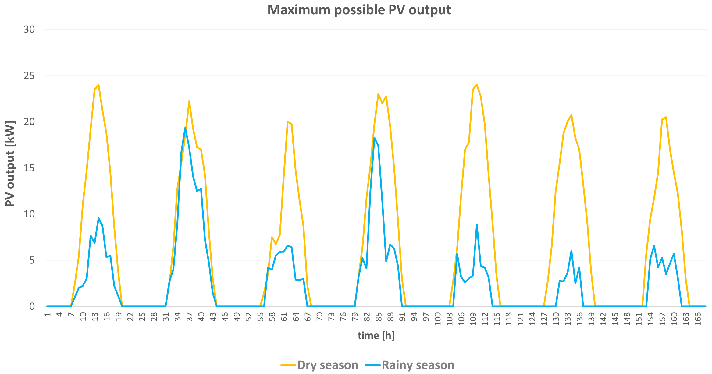
Figure A1.
Maximum PV output for a rainy and a dry season week for Section 5.
Figure A1.
Maximum PV output for a rainy and a dry season week for Section 5.

Figure A2.
Data Input for FiT and BPT for Section 5.
Figure A2.
Data Input for FiT and BPT for Section 5.

Figure A3.
Optimal dispatch for dry season off-grid mini-grid with extra reliability constraint of for Customer B.
Figure A3.
Optimal dispatch for dry season off-grid mini-grid with extra reliability constraint of for Customer B.

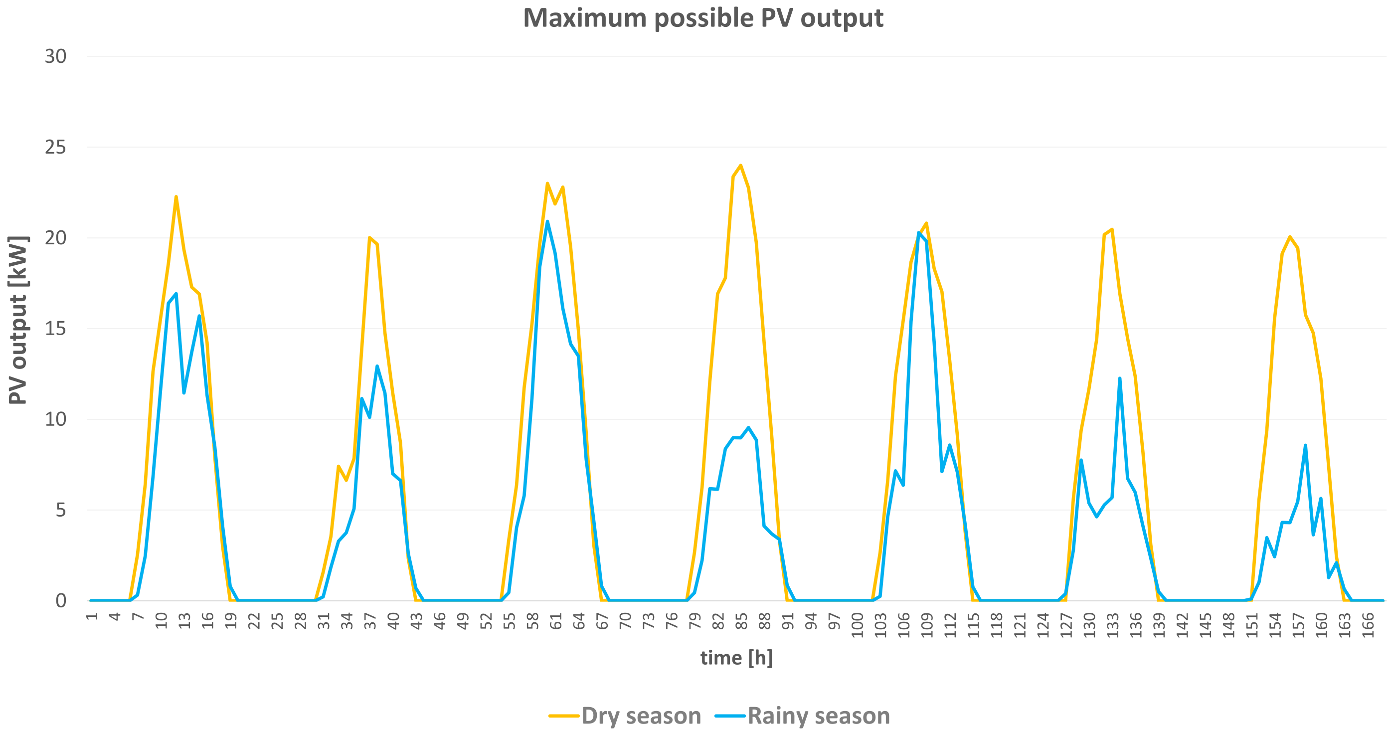
Figure A4.
Maximum PV output for a rainy and a dry season week for Section 6.
Figure A4.
Maximum PV output for a rainy and a dry season week for Section 6.

Figure A5.
Data Input Load A and B for Section 6.
Figure A5.
Data Input Load A and B for Section 6.

Figure A6.
Data Input for FiT and BPT for Section 6.
Figure A6.
Data Input for FiT and BPT for Section 6.

References
- IEA. Energy for All: Financing Access for the Poor; IEA: Paris, France, 2012. [Google Scholar]
- INENSUS. Mini-Grid Policy Toolkit; EU Energy Initiative Partnership Dialogue Facility (EUEI-PDF): Eschborn, Germany, 2014. [Google Scholar]
- Quanyua, J.; Meidong, X.; Guangchao, G. Energy Mangament of Microgrid in Grid-Connected and Stand-Alone modes. IEEE Trans. Power Syst. 2013, 28, 3380–3389. [Google Scholar] [CrossRef]
- Rocky Mountain Institute. Under the Grid: Improving the Economics and Reliability of Rural Electricity Service with Undergrid Minigrids. 2018. Available online: https://rmi.org/insight/under.the-grid/ (accessed on 15 January 2020).
- Hossain, M.A.; Pota, H.R.; Squartini, S.; Abdou, A.F. Modified PSO algorithm for real-time energy management in grid-connected microgrids. Renew. Energy 2019, 136, 746–757. [Google Scholar] [CrossRef]
- Lv, T.; Ai, Q.; Zhao, Y. A bi-level multi-objective optimal operation of grid-connected microgrids. Electr. Power Syst. Res. 2016, 131, 60–70. [Google Scholar] [CrossRef]
- Malysz, P.; Sirouspour, S.; Emadi, A. An Optimal Energy Storage Control Strategy for Grid-connected Microgrids. IEEE Trans. Smart Grid 2014, 5, 1785–1796. [Google Scholar] [CrossRef]
- International Energy Agency. Africa Energy Outlook; International Energy Agency: Paris, France, 2019; Available online: https://www.iea.org/reports/africa-energy-outlook-2019 (accessed on 15 January 2020).
- International Renewable Energy Agency. Innovation Outlook: Renewable Mini-Grids; International Renewable Energy Agency: Bonn, Germany, 2016. [Google Scholar]
- de Cuadra, F.; Perez-Arriaga, I.; Duenas, P. Towards Actionable Electrification Frameworks: Mini-Grids under the Grid; Instituto de Investigación Tecnologica (IIT) Working Paper; MIT Energy Initiative: Madrid, Spain, 2019. [Google Scholar]
- Ali, A.; Li, W.; Hussain, R.; He, X.; Williams, B.W.; Memon, A.H. Overview of Current Microgrid Policies, Incentives and Barriers in the European Union, United States and China. Sustainability 2017, 9, 1146. [Google Scholar] [CrossRef] [Green Version]
- Bauwens, T.; Gotchev, B.; Holstenkamp, L. What drives the development of community energy in Europe? The case of wind power cooperatives. Energy Res. Soc. Sci. 2016, 13, 136–147. [Google Scholar] [CrossRef]
- Ruiz, P.A.; Philbrick, C.R.; Zak, E.; Cheung, K.W.; Sauer, P.W. Uncertainty Management in the Unit Commitment Problem. IEEE Trans. Power Syst. 2009, 24, 642–651. [Google Scholar] [CrossRef]
- Takriti, S.; Birge, J.; Long, E. A stochastic model for the unit commitment problem. IEEE Trans. Power Syst. 1996, 11, 1497–1508. [Google Scholar] [CrossRef]
- Zhu, J. Optimization of Power System Operation, 2nd ed.; John Wiley and Sons, Inc.: New York, NY, USA, 2015. [Google Scholar] [CrossRef]
- Kirschen, D.; Strbac, G. Fundamentals of Power System Economics; John Wiley & Sons Ltd.: New York, NY, USA, 2004. [Google Scholar]
- Dennis Barley, C.; Byron Winn, C. Optimal dispatch strategy in remote hybrid power systems. Sol. Energy 1996, 58, 165–179. [Google Scholar] [CrossRef]
- Mandelli, S.; Barbieri, J.; Mereu, R.; Colombo, E. Off-grid systems for rural electrification in developing countries: Definitions, classification and a comprehensive literature review. Renew. Sustain. Energy Rev. 2016, 58, 1621–1646. [Google Scholar] [CrossRef]
- Burns, R. Optimization of Priority Lists for A Unit Commitment Program. In Proceedings of the IEEE Power Engineering Society Summer Meeting, San Francisco, CA, USA, 20–25 July 1975. [Google Scholar]
- H.O.M.E.R., 3.14. Hybrid Optimization of Multiple Energy Resources Software. Available online: https://www.homerenergy.com (accessed on 2 January 2020).
- Bernal-Agustín, J.L.; Dufo-López, R. Simulation and optimization of stand-alone hybrid renewable energy systems. Renew. Sustain. Energy Rev. 2009, 13, 2111–2118. [Google Scholar] [CrossRef]
- INENSUS. Billing, Revenue Collection and Metering Models for Mini-Grids. 2019. Available online: https://energy4impact.org/billing-revenue-collection-and-metering-models-mini-grids-0 (accessed on 8 November 2020).
- INENSUS. MicroPowerManager Software. Available online: https://micropowermanager.com (accessed on 10 July 2021).
- Mazzola, S.; Vergara, C.; Astolfi, M.; Li, V.; Perez-Arriaga, I.; Macchi, E. Assessing the value of forecast-based dispatch in the operation of off-grid rural microgrids. Renew. Energy 2017, 108, 116–125. [Google Scholar] [CrossRef]
- Ahmad Khan, A.; Naeem, M.; Iqbal, M.; Qaisar, S.; Anpalagan, A. A compendium of optimization objectives, constraints, tools and algorithms for energy management in microgrids. Renew. Sustain. Energy Rev. 2016, 58, 1664–1683. [Google Scholar] [CrossRef]
- Maciejowski, J. Predictive Control with Constraints; Prentice Hall: Harlow, UK, 2002. [Google Scholar]
- Morari, M.; Lee, J.H. Model Predictive Control: Past, Present and Future. Comput. Chem. Eng. 1997, 23, 667–682. [Google Scholar] [CrossRef]
- Ellis, M.; Durand, H.; Christofides, P.D. A tutorial review of economic model predictive control methods. J. Process. Control 2014, 24, 1156–1178. [Google Scholar] [CrossRef]
- Bordons, C.; Garcia-Torres, F.; Ridao, M. Model Predictive Control of Microgrids; Springer Nature Switzerland AG: Cham, Switzerland, 2020. [Google Scholar]
- Hu, J.; Shan, Y.; Guerrero, J.M.; Ioinovici, A.; Chan, K.W.; Rodriguez, J. Model predictive control of microgrids—An overview. Renew. Sustain. Energy Rev. 2021, 136, 110422. [Google Scholar] [CrossRef]
- Aloo, L.A.; Kihato, P.K.; Kamau, S.I.; Orenge, R.S. Model Predictive Control-Adaptive Neuro-Fuzzy Inference System Control Strategies for Photovoltaic-Wind Microgrid: Feasibility Review. In Proceedings of the 2020 IEEE PES/IAS PowerAfrica, Nairobi, Kenya, 25–28 August 2020; pp. 1–5. [Google Scholar] [CrossRef]
- Mbungu, N.T.; Naidoo, R.; Bansal, R.C.; Bipath, M. Optimisation of grid connected hybrid photovoltaic–wind–battery system using model predictive control design. IET Renew. Power Gener. 2017, 11, 1760–1768. [Google Scholar] [CrossRef]
- Taha, M.S.; Mohamed, Y.A.R.I. Robust MPC-based energy management system of a hybrid energy source for remote communities. In Proceedings of the 2016 IEEE Electrical Power and Energy Conference (EPEC), Ottawa, ON, Canada, 12–14 October 2016; pp. 1–6. [Google Scholar] [CrossRef]
- Siti, M.W.; Tiako, R.; Bansal, R. A model predictive control strategy for grid-connected solar-wind with pumped hydro storage. In Proceedings of the 5th IET International Conference on Renewable Power Generation (RPG) 2016, London, UK, 21–23 September 2016; pp. 1–6. [Google Scholar] [CrossRef]
- Kim, S.K.; Kim, J.Y.; Cho, K.H.; Byeon, G. Optimal Operation Control for Multiple BESSs of a Large-Scale Customer under Time-Based Pricing. IEEE Trans. Power Syst. 2018, 33, 803–816. [Google Scholar] [CrossRef]
- Schmitt, T.; Rodemann, T.; Adamy, J. The Cost of Photovoltaic Forecasting Errors in Microgrid Control with Peak Pricing. Energies 2021, 14, 2569. [Google Scholar] [CrossRef]
- Basu, A.K.; Bhattacharya, A.; Chowdhury, S.; Chowdhury, S.P. Planned Scheduling for Economic Power Sharing in a CHP-Based Micro-Grid. IEEE Trans. Power Syst. 2012, 27, 30–38. [Google Scholar] [CrossRef]
- Conti, S.; Nicolosi, R.; Rizzo, S.A.; Zeineldin, H.H. Optimal Dispatching of Distributed Generators and Storage Systems for MV Islanded Microgrids. IEEE Trans. Power Deliv. 2012, 27, 1243–1251. [Google Scholar] [CrossRef]
- Ding, Z.; Lee, W.J. A Stochastic Microgrid Operation Scheme to Balance Between System Reliability and Greenhouse Gas Emission. IEEE Trans. Ind. Appl. 2016, 52, 1157–1166. [Google Scholar] [CrossRef]
- Hernandez-Aramburo, C.; Green, T.; Mugniot, N. Fuel consumption minimization of a microgrid. IEEE Trans. Ind. Appl. 2005, 41, 673–681. [Google Scholar] [CrossRef] [Green Version]
- Kamankesh, H.; Agelidis, V.G.; Kavousi-Fard, A. Optimal scheduling of renewable micro-grids considering plug-in hybrid electric vehicle charging demand. Energy 2016, 100, 285–297. [Google Scholar] [CrossRef]
- Parhizi, S.; Khodaei, A. Market-based microgrid optimal scheduling. In Proceedings of the 2015 IEEE International Conference on Smart Grid Communications, Miami, FL, USA, 2–5 November 2015; pp. 55–60. [Google Scholar] [CrossRef] [Green Version]
- Wang, R.; Wang, P.; Xiao, G. A robust optimization approach for energy generation scheduling in microgrids. Energy Convers. Manag. 2015, 106, 597–607. [Google Scholar] [CrossRef]
- Wu, X.; Wang, X.; Qu, C. A Hierarchical Framework for Generation Scheduling of Microgrids. IEEE Trans. Power Deliv. 2014, 29, 2448–2457. [Google Scholar] [CrossRef]
- Chowdhury, S.; Crossley, P. Microgrids and Active Distribution Networks; Institution of Engineering and Technology: London, UK, 2009. [Google Scholar]
- Richter, C.; Sheble, G. A profit-based unit commitment GA for the competitive environment. IEEE Trans. Power Syst. 2000, 15, 715–721. [Google Scholar] [CrossRef]
- Tahanan, M.; van Ackooij, W.; Frangioni, A. Large-scale Unit Commitment under uncertainty. J. Oper. Res. 2015, 13, 115–171. [Google Scholar] [CrossRef] [Green Version]
- Wu, Y.K.; Ye, G.T.; Tang, K.T. Preventive Control Strategy for an Island Power System That Considers System Security and Economics. IEEE Trans. Ind. Appl. 2017, 53, 5239–5251. [Google Scholar] [CrossRef]
- Dolara, A.; Grimaccia, F.; Magistrati, G.; Marchegiani, G. Optimization Models for Islanded Micro-Grids: A Comparative Analysis between Linear Programming and Mixed Integer Programming. Energies 2017, 10, 241. [Google Scholar] [CrossRef]
- Morais, H.; Kádár, P.; Faria, P.; Vale, Z.A.; Khodr, H. Optimal scheduling of a renewable micro-grid in an isolated load area using mixed-integer linear programming. Renew. Energy 2010, 35, 151–156. [Google Scholar] [CrossRef] [Green Version]
- Bard, J.F. Short-Term Scheduling of Thermal-Electric Generators Using Lagrangian Relaxation. Oper. Res. 1988, 36, 756–766. [Google Scholar] [CrossRef]
- GAMS Development Corporation. General Algebraic Modeling System. 2007. Available online: http://www.gams.com/ (accessed on 4 January 2020).
- NASA. Prediction of Worldwide Energy Resource. 2020. Available online: http://power.larc.nasa.gov (accessed on 5 December 2020).
Figure 1.
Configuration of an undergrid mini-grid.

Figure 2.
Topology of a mini-grid under the grid.

Figure 3.
Different possible hourly UMG demand and offer bids.

Figure 4.
Evaluation of a demand bid in the present and supply bid in the future market.

Figure 5.
Total welfare in a UC objective function without predetermined (left) and with predefined (right).
Figure 5.
Total welfare in a UC objective function without predetermined (left) and with predefined (right).

Figure 6.
Model-predictive control for UMG market-based optimal scheduling.

Figure 7.
UMG optimal dispatch for dry season and full grid.

Figure 8.
UMG optimal dispatch for dry season and unreliable grid.

Figure 9.
UMG optimal dispatch for rainy season and full grid.

Figure 10.
UMG optimal dispatch for rainy season and unreliable grid.

Figure 11.
Optimal dispatch for dry season off-grid mini-grid.

Figure 12.
Optimal dispatch for rainy season off-grid mini-grid.

Figure 13.
HOMER Pro’s LF strategy for dry season full grid.

Figure 14.
Market-based optimal dispatch for dry season full grid.

Figure 15.
HOMER Pro’s LF strategy for rainy season Unreliable Grid.

Figure 16.
Market–based optimal dispatch for rainy season unreliable grid.

Figure 17.
HOMER Pro’s CC strategy for dry season unreliable grid.

Figure 18.
Market-based optimal dispatch for dry season unreliable grid.

Figure 19.
Market–based optimal dispatch for dry season off-grid mini-grid.

Figure 20.
HOMER Pro’s predictive strategy for dry season off-grid mini-grid.

Figure 21.
Market–based optimal dispatch for dry season off-grid mini-grid with extra reliability constraint for load B.
Figure 21.
Market–based optimal dispatch for dry season off-grid mini-grid with extra reliability constraint for load B.

Table 1.
Result summary table for scenarios in the dry season.
| Dry Season (48 h) | |||
|---|---|---|---|
| Scenarios | Full Grid | Unreliable Grid | Off-Grid |
| Total Welfare ($) | 182 | 179 | 150 |
| Operat. Costs ($) | −25 | −24 | −18 |
| Total Served Demand (kWh) | 679 | 664 | 459 |
| MG Generation (kWh) | 464 | 482 | 488 |
| Grid Import (kWh) | 244 | 213 | 0 |
| Total shortage (kWh) | 0 | 19 | 141 |
| Overall reliability (%) | 100 | 96 | 69 |
| Reliability of Load B (%) | 100 | 89 | 15 |
Table 2.
Result summary table for scenarios in the rainy season.
| Rainy Season (48 h) | |||
|---|---|---|---|
| Scenarios | Full Grid | Unreliable Grid | Off-Grid |
| Total Welfare ($) | 173 | 171 | 146 |
| Operat. Costs ($) | −37 | −37 | −54 |
| Total Served Demand (kWh) | 610 | 591 | 371 |
| MG Generation (kWh) | 317 | 328 | 385 |
| Grid Import (kWh) | 321 | 292 | 0 |
| Total shortage (kWh) | 0 | 19 | 165 |
| Overall reliability (%) | 100 | 96 | 64 |
| Reliability of Load B (%) | 100 | 89 | 0 |
Table 3.
Comparison table for simulation results under dry season with a reliable main grid.
| Dry Season–Full Grid (48 h) | ||
|---|---|---|
| Simulations | Homer Pro LF | Market Dispatch |
| Total Welfare ($) | 136 | 143 |
| Operat. Costs ($) | −43 | −35 |
| Total Served Demand (kWh) | 531 | 631 |
| MG Generation (kWh) | 275 | 275 |
| Grid Import (kWh) | 228 | 248 |
| Total shortage (kWh) | 0 | 13 |
| Overall reliability (%) | 100 | 97 |
| Reliability of Load B (%) | 100 | 91 |
| RE fraction on MG demand (%) | 67.1 | 67.2 |
Table 4.
Comparison table for simulation results under rainy season with an unreliable main grid.
| Rainy Season–Unreliable Grid (48 h) | ||
|---|---|---|
| Simulations | Homer Pro LF | Market Dispatch |
| Total Welfare ($) | 119 | 124 |
| Operat. Costs ($) | −47 | −38 |
| Total Served Demand (kWh) | 481 | 577 |
| MG Generation (kWh) | 249 | 197 |
| Grid Import (kWh) | 196 | 248 |
| Total shortage (kWh) | 1 | 22 |
| Overall reliability (%) | 99.7 | 94.6 |
| Reliability of Load B (%) | 99.3 | 85.7 |
| RE fraction on MG demand (%) | 47.6 | 50.9 |
Table 5.
Comparison table for simulation results under rainy season with an unreliable main gird.
| Dry Season—Unreliable Grid-Increased Load (48 h) | ||
|---|---|---|
| Simulations | Homer Pro CC | Market Dispatch |
| Total Welfare ($) | 201 | 224 |
| Operat. Costs ($) | −85 | −55 |
| Total Served Demand (kWh) | 748 | 732 |
| MG Generation (kWh) | 291 | 275 |
| Grid Import (kWh) | 377 | 312 |
| Total shortage (kWh) | 0 | 75 |
| Overall reliability (%) | 100 | 89 |
| Reliability of Load B (%) | 100 | 51 |
| RE fraction on MG demand (%) | 37.6 | 46.6 |
Table 6.
Comparison table for simulation results under the dry season isolated MG.
| Dry Season–Isolated MG (48 h) | |||
|---|---|---|---|
| Simulations | Homer PS | Market Dispatch | MD 100% Reliability |
| Total Welfare ($) | 89 | 112 | 96 |
| Operat. Costs ($) | −68 | −21 | −62 |
| Total Served Demand (kWh) | 578 | 402 | 492 |
| MG Generation (kWh) | 454 | 310 | 450 |
| Grid Import (kWh) | 0 | 0 | 0 |
| Total shortage (kWh) | 0 | 131 | 0 |
| Overall reliability (%) | 100 | 68 | 100 |
| Reliability of Load B (%) | 100 | 15 | 100 |
| RE fraction on MG demand (%) | 67.1 | 98.8 | 67.2 |
Publisher’s Note: MDPI stays neutral with regard to jurisdictional claims in published maps and institutional affiliations. |
© 2021 by the authors. Licensee MDPI, Basel, Switzerland. This article is an open access article distributed under the terms and conditions of the Creative Commons Attribution (CC BY) license (https://creativecommons.org/licenses/by/4.0/).
Share and Cite
MDPI and ACS Style
González Grandón, T.; de Cuadra García, F.; Pérez-Arriaga, I. A Market-Driven Management Model for Renewable-Powered Undergrid Mini-Grids. Energies 2021, 14, 7881. https://doi.org/10.3390/en14237881
AMA Style
González Grandón T, de Cuadra García F, Pérez-Arriaga I. A Market-Driven Management Model for Renewable-Powered Undergrid Mini-Grids. Energies. 2021; 14(23):7881. https://doi.org/10.3390/en14237881
Chicago/Turabian StyleGonzález Grandón, Tatiana, Fernando de Cuadra García, and Ignacio Pérez-Arriaga. 2021. "A Market-Driven Management Model for Renewable-Powered Undergrid Mini-Grids" Energies 14, no. 23: 7881. https://doi.org/10.3390/en14237881
Note that from the first issue of 2016, this journal uses article numbers instead of page numbers. See further details here.