
Volatility and Dispersion of Hourly Electricity Contracts on the German Continuous Intraday Market

Chair of Banking and Finance, University of Hagen, Universitätsstraße 41, 58084 Hagen, Germany
*
Author to whom correspondence should be addressed.
Energies 2021, 14(22), 7531; https://doi.org/10.3390/en14227531
Submission received: 6 October 2021
/
Revised: 5 November 2021
/
Accepted: 7 November 2021
/
Published: 11 November 2021
Abstract
:Intraday electricity trading on the continuous intraday market of EPEX SPOT is particularly well suited for the rebalancing of energy production. We analyzed the volatility and dispersion of individual hourly contracts, taking into account the particularities of the market, due to which the standard volatility measure from financial time series cannot be applied. We used and analyzed five measures for price fluctuations, which turned out to be similarly well suited for electricity contracts, with small differences. We then identified fundamental drivers of price fluctuations: the relative share of wind in the overall mix increased dispersion. In addition, price dispersion was positively correlated with the traded volume as well as the absolute difference between the day-ahead auction price and the volume-weighted intraday price. We furthermore analyzed the timely structure of price fluctuations to identify forecast indicators for a contract’s peak trading hour before maturity, finding that trading-related variables are more important to forecast price fluctuations than fundamental factors. With lagged realizations and additional external drivers, forecast regressions reached an adjusted of 0.479 for volatility and around 0.3 for the dispersion measures.
Keywords:
intraday electricity market; renewable energies; electricity price volatility; electricity price dispersionJEL Classification:
C20; Q40; Q41; Q421. Introduction
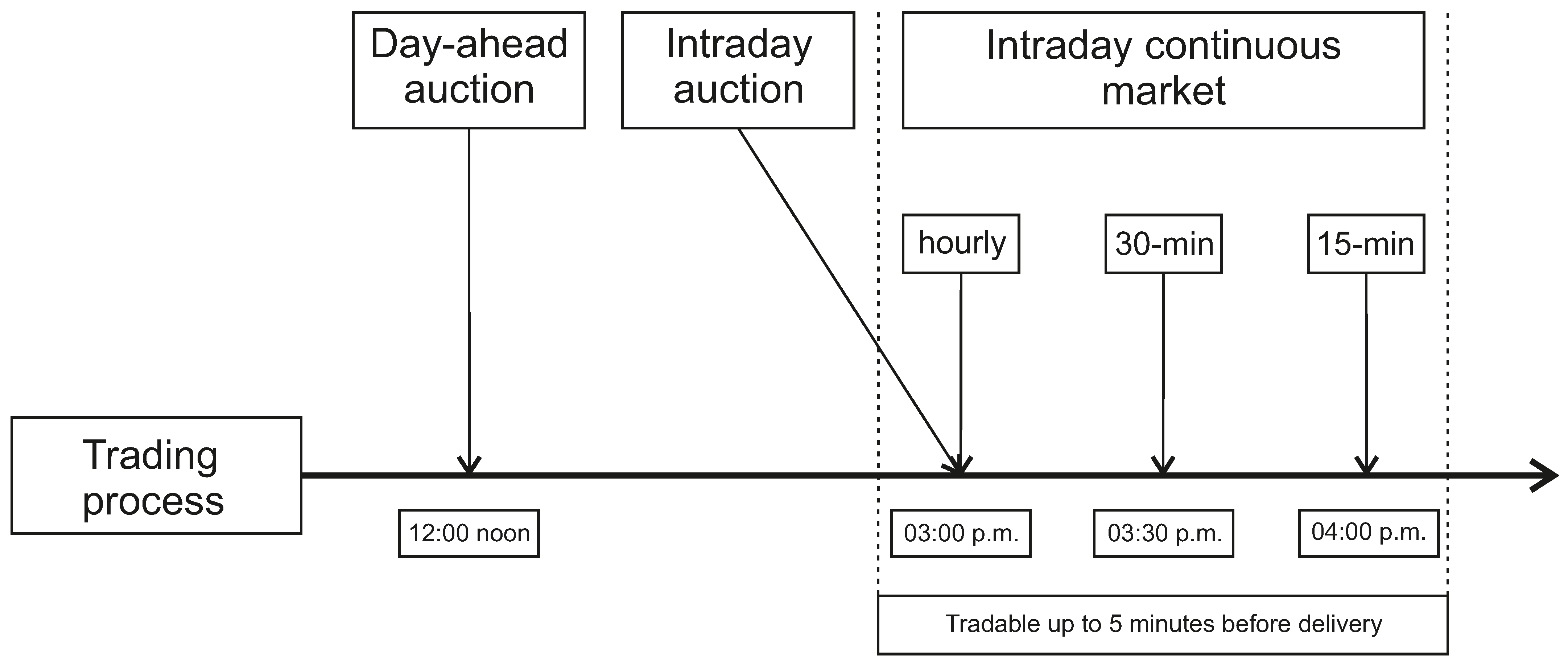
Short-term trading of electricity in Germany mainly takes place at the EPEX SPOT exchange. Basically, there are two types of markets to fulfill different needs: the day-ahead auction offers the opportunity to adjust the production schedule for the following day with regard to hourly contracts and takes place at 12 a.m. each day. However, this does not allow market participants to react quickly to changes in forecasts for renewable energies, particularly wind and solar energy. This possibility is offered by the continuous intraday market, which starts at 3 p.m. each day for hourly contracts for the following day. Furthermore, 30-min and 15-min contracts are offered. Besides the day-ahead auction and the continuous intraday market, there is the intraday auction at 3 p.m. each day for 15-min contracts for the following day. Continuous trading is possible up to 5 min before the start of the traded period. Until 2020, the contracts were tradeable up to 30 min before delivery. Only within the respective control areas was extended trading already possible since June 2017. In Germany, there are four such control zones or transmission systems, which guarantee the infrastructure of the transregional electricity grids. Figure 1 shows the structure of a trading day on EPEX SPOT.
Recent years have experienced a steady increase in trading volume in the continuous intraday market, which has thus gained importance compared to the day-ahead market. In 2020, the total trading volume of German intraday contracts at EPEX SPOT reached 64 TWh, amounting to 23% of the overall German trading volume, with hourly contracts accounting for the largest part.
The main goal of this study was to analyze price fluctuations on the continuous market and their drivers. While most contributions in the literature focus on the day-ahead market, we are the first to provide a comprehensive overview of price fluctuations of individual hourly contracts during their (short-dated) lifetime. In this regard, the concept of “volatility” is used in different ways in the literature. Most authors, such as [1,2], analyze price differences between different contracts, for example, the day-ahead prices of the 00h–01h contract, the 01h–02h contract, the 02h–03h contract, etc. Additionally, studies focusing on the intraday market, e.g., [3], analyze such price differences between different contracts, referring to average prices for a single contract during its lifetime. However, the original idea of volatility, known from financial time-series, refers to price fluctuations of the same contract. In the context of electricity trading, these are fluctuations of intraday prices for an individual contract, with a trading window from 3 p.m. until the traded hour on the next day. The extent of this intraday price fluctuations is of particular importance for both suppliers and demanders of energy, who have to react to short-term deviations from their anticipated buy or sell volume. They settle their needs at the intraday market and are thus exposed to intraday price risk. We analyzed patterns of intraday electricity price fluctuations in terms of volatility (taking the timely structure of trades into account) and dispersion (ignoring this timely structure), detecting contractual and seasonal differences.
Due to the differences between the continuous intraday market and financial markets, the application of the classical measure of volatility, defined as the (annualized) standard deviation of log returns over equal periods of time, is hardly feasibly. One problem is the occurrence of negative prices, which prevents calculating log returns. Furthermore, the intraday price series turn out to exhibit extreme movements (“spikes”) for single trades, often with low trading volume. Since the classical definition of volatility is based on the assumption of a continuous diffusion process, spikes would cause classical volatility to become extremely large when the observation frequency is based on small intraday time intervals (e.g., on a minute basis). Our first contribution was therefore to analyze different appropriate price fluctuation measures, which take into account the special features of the continuous intraday market. We used five different measures. One measure, similar to [4], considers price differences of consecutive trades and is thus most similar to classical volatility. The other four do not make use of the time structure of the intraday trades but are statistical dispersion measures of the set of trading prices for a single contract during its (short-termed) lifetime.
We did not analyze potential advantages or disadvantages of the selected price fluctuation measures but the relationships between them. The five measures focus on different aspects and differ in their robustness against outliers. Nonetheless, we found that they behave quite similarly and concluded that the choice of a particular measure is of minor importance. Roughly speaking, the average intraday price fluctuation amounts to about 10% of the trading price.
Equipped with these measures, as the second contribution of this study, we then analyzed potential drivers of intraday price fluctuations for the hourly contracts. With different regression designs, we found that especially the relative share of wind in the overall energy mix and the traded volume are related to price fluctuations but that the share of solar energy has little to no impact.
The third contribution consists of identifying forecasting variables for price fluctuations during the last trading hour of a single contract. During this last hour, nearly half of the total volume is traded. Analyzing correlations between fluctuation measures of succeeding contracts, we showed that the realized volatility and dispersion of expired contracts can be used to forecast future price fluctuations. Together with external parameters, particularly the current share of wind energy, the forecasting regressions reached an adjusted of 0.479 for absolute volatility and around 0.3 for different dispersion measures. We showed that trading-related variables have a greater influence than fundamental factors.
2. Literature Review
Early analyses for the day-ahead market regarding the impact of wind energy on electricity prices by [5,6] concluded that the feed-in of wind energy reduces prices and induces a change in the merit order, as the marginal costs of renewable energies production are almost zero. The merit order ranks available power generation in ascending order of price, based on the lowest marginal costs and amount being produced. In addition, [5,6] expect a general increase in volatility on electricity markets.
Wind energy reduces prices at the German day-ahead auction and increases volatility, as was confirmed by [7,8,9], among others. The same findings reported [10] for the Italian electricity market. An analysis of wind and solar energy shocks by [1] concluded that wind energy shocks have a longer negative effect on spot prices than solar energy shocks. For the Danish and German spot market, [2] analyzed the influence of renewable energies on spot volatilities. While in Denmark volatility is reduced by wind energy, it is increased in the German market because it has a greater influence on off-peak prices. Solar energy, on the other hand, reduces volatility.
Another strand of literature compares the energy prices at the day-ahead auction with those on the continuous intraday market or analyzes both. Conducting a price analysis using fundamentals by [11], they identified (avoided) start-up costs, market states, and trading behavior as drivers for the differences between the predicted prices and the observed prices. Using panel data, the effects of wind and solar energy were analyzed by [12]. They found price-dampening effects from both wind and solar energy on electricity prices, though the effects have been reduced since 2013 due to falling fuel prices. In addition, a reduction in forecast errors regarding wind and solar energy has led to lower price volatility. Improved forecasts of fundamentals lead to more accurate day-ahead and intraday prices, as shown by [13], and [14] used principal component analysis to forecast both prices.
With respect exclusively to the continuous intraday market and 15-min contracts, bidding strategies have been analyzed by [15], among others, regarding forecasting errors of solar and wind energy. With price forecasts of 15-min-contracts [16] dealt, and [3] forecast realized volatilities on the continuous intraday market. The influence of the introduction of 15-min contracts on the existing hourly contracts was analyzed by [17]. They found evidence that the prices of hourly contracts decreased and that the 15-min contracts are used to balance intra-hour fluctuations of renewable energies. A variable selection for price drivers was performed by [18], and [19] analyzed the impact of errors in wind and solar power forecasts for very short-term electricity price forecasting.
All these studies were based on volume-weighted prices of quarter-hourly, hourly contracts or the volume-weighted average price of all continuous trades executed within the last 3 trading hours of a contract on the continuous intraday market (). Most closely related to our study are contributions that consider the contracts of the continuous intraday market individually. A detailed analysis of the 15-min individual contracts on the continuous intraday market was provided by [4]. With regard to volatility, they used data from observed trades for a 15-min contract and calculated the difference between consecutive prices as the basis for price fluctuations. Further price analysis of 15-min contracts was also performed by [20,21]. Forecasting price distributions of hourly contracts over quantiles that occur in the last 3 h before delivery was the focus of [22]. Thus, in a sense, the range of quantiles also captures the dispersion of contract prices. The transnational trading of the continuous intraday market was addressed by [23], who defined the dispersion as the volume-weighted standard deviation of individual transactions. An analysis of the prices of the individual contracts, considering the individual trades, was carried out by [24], and [25] were engaged in price forecasting of hourly contracts. A mathematical model for intraday power trading that involves both renewable and conventional generation was presented by [26]. Finally, the arrival of orders for the continuous intraday market was analyzed by [27].
3. Data and Methodology
3.1. Data
The data set provided by EPEX SPOT contains the individual trades of the hourly contracts on the continuous intraday market in the period from October 2015 through September 2018. Thus, the raw data set covers a total of 1,090 days (36 months) with the corresponding 24 hourly contracts. We removed those days on which a clock change had taken place (from standard time to daylight saving time or vice versa), because otherwise a contract was duplicated or missing. Additionally, a total of 152 contracts with no transaction data in the last hour until maturity were excluded.
For each trade, the trading price, the time stamp on a minute basis, the volume, the buy country, and the sell country are available. As we were interested in price fluctuations on the German market, we removed all trades from the data set in which the German market was not involved. Furthermore, we did not consider transactions that were executed within a control zone in the last 30 min until delivery, since, first, this opportunity was not available during the entire sample period, and, second, those transactions are not directly comparable due to the regional limitation.
To determine possible drivers of price fluctuations, we furthermore needed different fundamentals of the German electricity market. In addition to price data of the day-ahead auction provided by EPEX SPOT, we used a data set from the German Network Agency. The data sets are available on www.smard.de (accessed on 5 November 2018). First, this data set contains information about the generation of renewable energies in Germany. The information is available for both realized and forecasted solar and wind energy in quarter-hourly time intervals. Second, the data set contains data on the total electricity generated as well as consumed in Germany. The forecasts for the following day of each electricity generation are published until 6 p.m., while the forecasts for electricity consumption are already published until 10 a.m. The data set is not complete for all fundamentals. In cases of missing data, we excluded the respective contract(s) from the analysis.
After data cleanup, 25,104 contracts out of 1090 × 24 = 26,160 contracts remained for the analysis of price fluctuation drivers. For these contracts, we analyzed a total number of million transactions.
3.2. Measures of Price Fluctuations
The classical measure of volatility, known from financial time series, is defined as the (annualized) standard deviation of log returns over equal periods of time:
For diffusion processes that are common in the modeling of financial time series (e.g., geometric Brownian motion), estimating volatility does not depend on the observation frequency . However, when prices exhibit extreme movements (“spikes”), volatility estimators can become extremely large, because large log returns occur in small intervals . Furthermore, the calculation of log returns requires consistently positive prices.
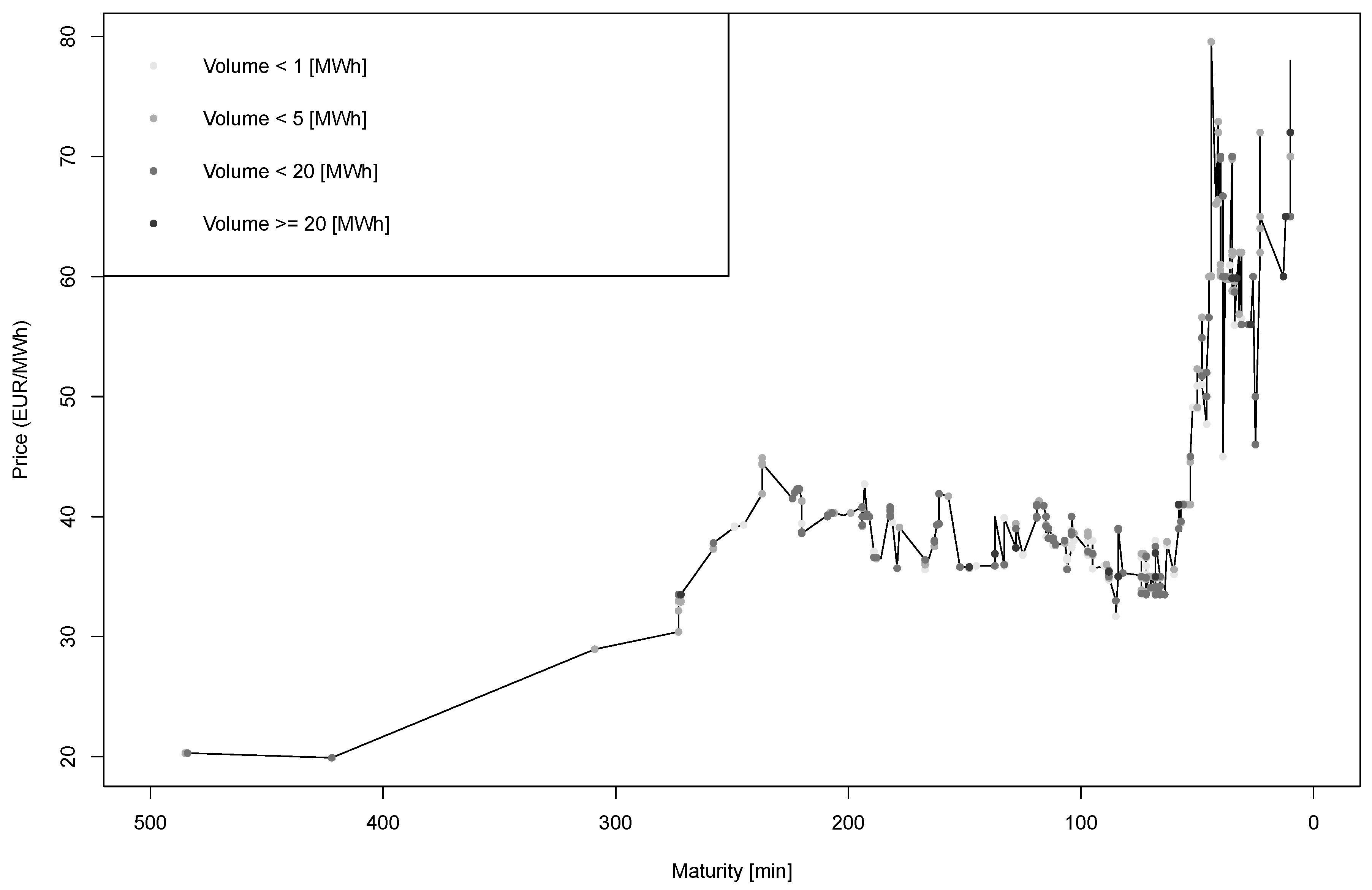
Figure 2 shows the price development for a randomly selected exemplary contract, the 00 h–01 h contract on 23 September 2018. The figure illustrates some differences between a stock market and the continuous intraday market for electricity. The special features of the electricity market, for example, lack of storage capacities, can lead to short-term price spikes (including negative prices) on the spot markets if demand and production do not match. See [28] for more stylized facts in electricity markets. The market gives participants the opportunity to react quickly to changes and thus to carry out an hourly rebalancing of the electricity portfolio. The graph shows large price movements from about EUR 20 to 80 per MWh within the few hours of trading. Furthermore, trades are unevenly distributed and cluster at the end of the period. We consider trading until 30 min before delivery. Trading within the control zones afterwards is neglected.
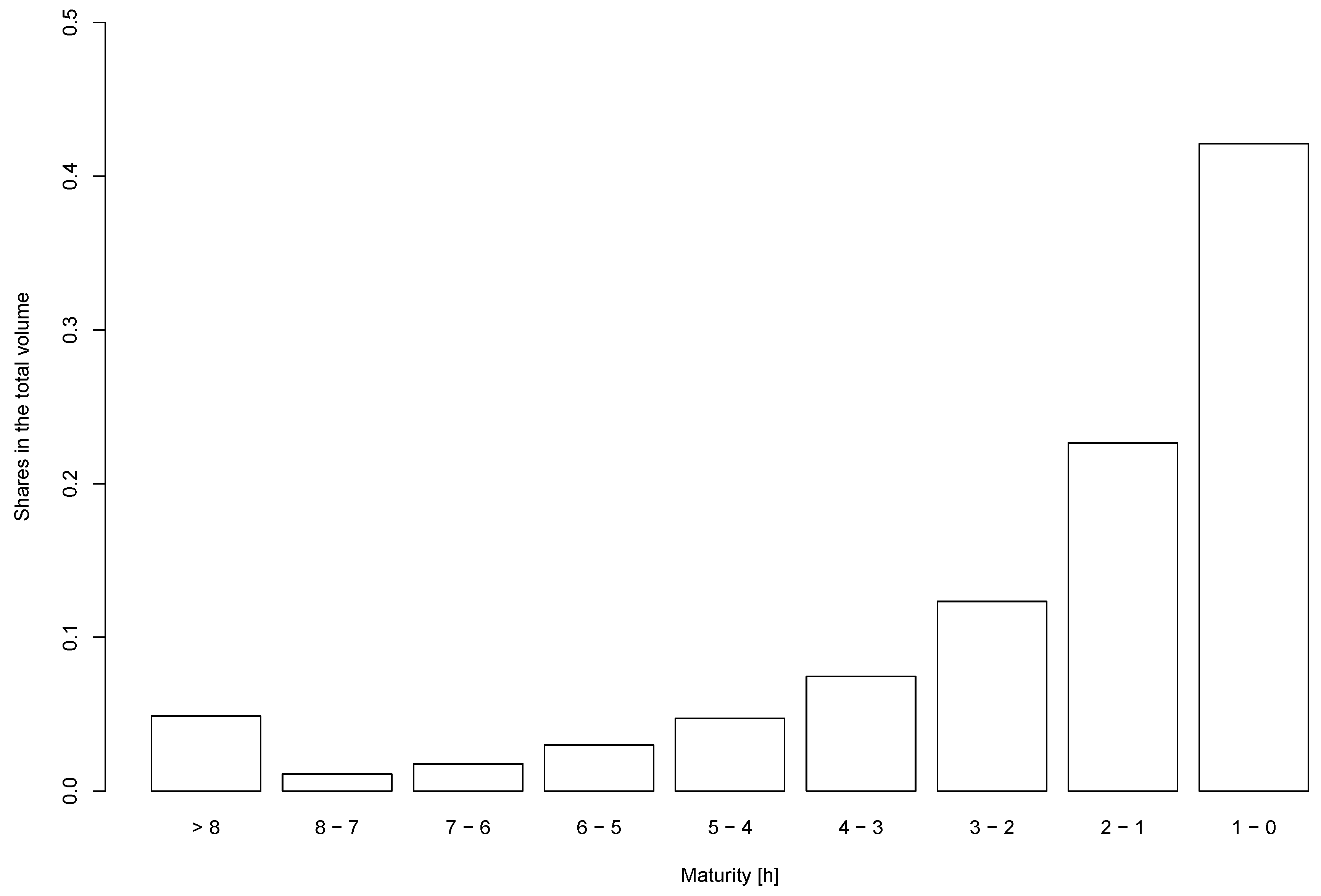
Figure 3 shows the distribution of the trading volume within the lifetime of the contracts. In line with the observations of [24,29] for the Spanish and German continuous intraday markets, the trading volume increases with decreasing maturity. On average, more than 40% of the total volume is traded in the last hour before maturity.
Because of negative prices, price peaks and the asymmetric distribution of trading volume, a classical measure of volatility, were not appropriate for the intraday electricity market. About two percent of all realized prices on the continuous intraday market were negative during the observation period. Instead, we propose three different categories of volatility and dispersion measures, which cover a variety of different statistical approaches to measure and analyze price fluctuations. The first category is similar to the classical volatility, as we measured the differences between successive trade prices. However, we neglected the time difference and measured the absolute deviations between consecutive trades. In the other two categories, we dropped any time structure of the intraday trades and considered the trading prices of each single contract as a set of price information without time stamps and measured the dispersion. In the second category, we considered deviations around the mean, and in the third category we used ranges. Various other measures were also tested, including outlier-adjusted measures, mean absolute deviations for Categories A and B, and further ranges for Category C. As for notation, a contract is defined via the index pair h for the delivery hour and d for the calendar date. The index t denotes the number of a trade for an individual contract; is the number of trades for a contract, is the price of a single trade, and the traded volume. The five measures are defined as follows.
A. Volatility-like measure
- The absolute volatility as the standard deviation of price differences of two consecutive trades:This measure is inspired by [4].
B. Dispersion measures
- 2.
- The simple standard deviation of prices:
- 3.
- The volume-weighted standard deviation of prices:The volume-weighted standard deviation is also proposed by [23].
C. Range measures
- 4.
- The total range:The usability of ranges as a proxy for intraday volatility in stock markets was shown by [30].
- 5.
- The interquartile range:where is the (generalized) inverse of the empirical volume-weighted price distribution for contract (h, d).
3.3. Descriptive Statistics
Table 1 shows some descriptive statistics of the five measures for total price fluctuations (Panel A) and price fluctuations in the last hour before maturity. For example, the last hour before maturity for the 00h–01h contract refers to the period from 10:30 p.m. to 11:30 p.m. (Panel B). Over all contracts, the total average price difference between two consecutive trades was about EUR 0.88 per MWh (), while the average standard deviation amounted to about EUR 3.41 per MWh ( and ) of electricity. The average total price range of a contract was about EUR 18 per MWh () and the average interquartile range about EUR 4.40 per MWh (). All five measures show an extreme right-skewness and a very high kurtosis. The different categories exhibit medium-to-high correlations with values of ( and ) and ( and ) for the measures of the same category. The relatively low correlation between the ranges is explained by the extreme values of the measure . As expected, the price fluctuations in the last hour before maturity and their standard deviations are smaller in comparison.
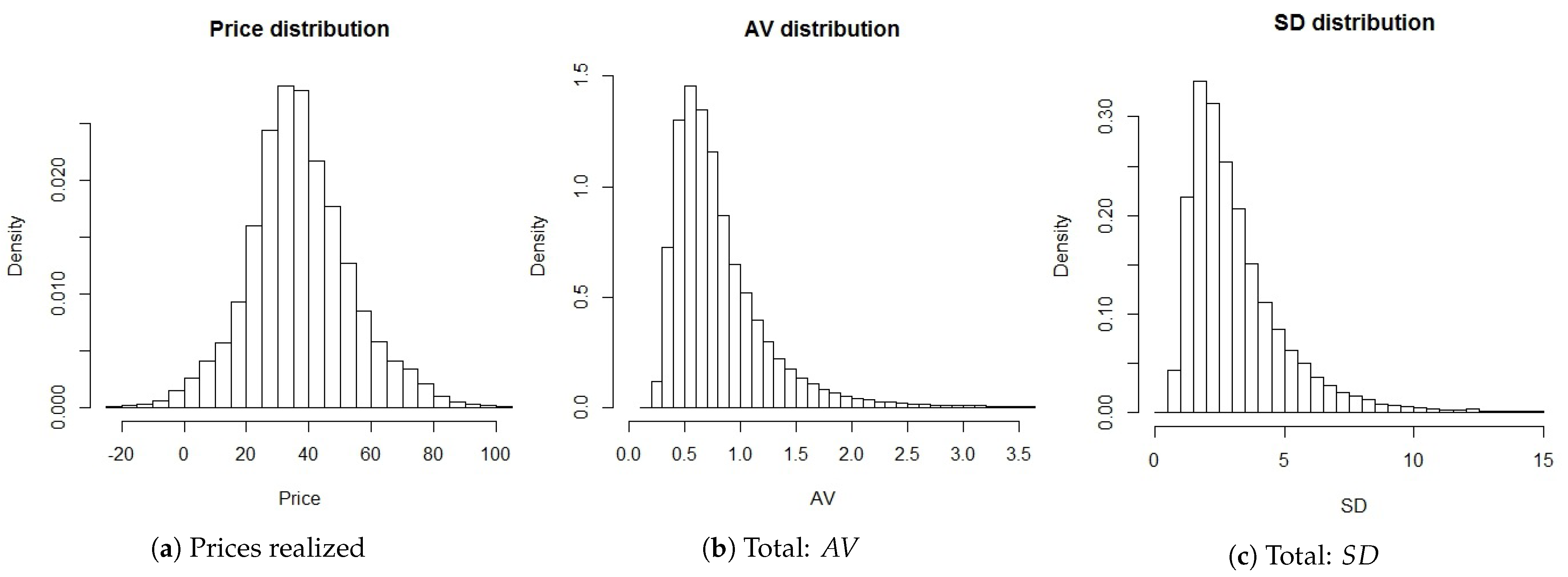
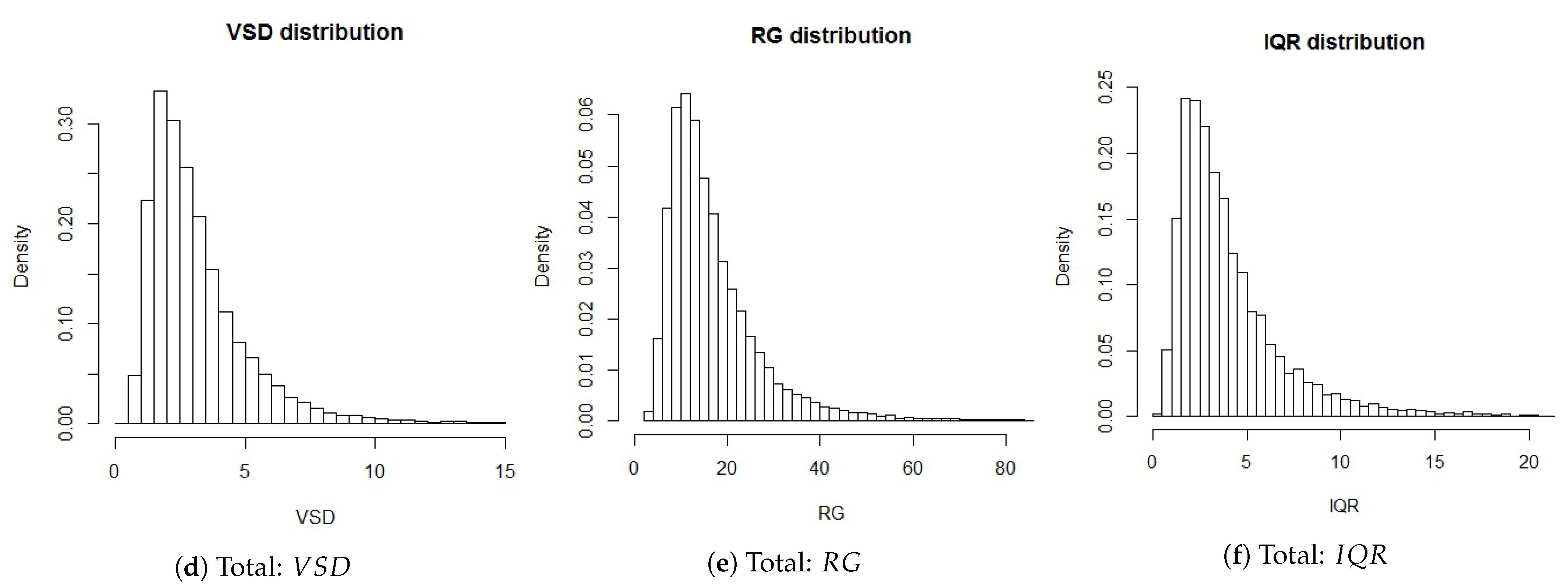
An additional overview of the distributions of the prices as well as the different price fluctuation measures is provided by Figure 4. Figure 4a shows the distribution of all realized prices in the entire data set across all contracts. The extreme values at the tails of the distributions were omitted for clarity, since the maximum observed price was EUR 4100 per MWh, and the minimum price was EUR −1000 per MWh. The five measures of total price fluctuation are illustrated in Figure 4b–f. Extreme values on the right-hand side of the figure were also omitted.
For our following analysis of the potential drivers of price fluctuations, the extremely high values for skewness and kurtosis indicate potential problems with outliers. For this reason, we logarithmized the price fluctuation measures. Furthermore, in line with similar approaches in the literature (e.g., [31,32]), we identified outliers by standard deviation and excluded values that exceeded four times the standard deviation around the mean for each measure. The method for selecting possible outliers is of high importance for electricity prices, e.g., [33,34]. We therefore checked several other approaches (no outliers removal, three standard deviations, different percentage filters). None of these approaches resulted in different conclusions than those presented below. Accordingly, our presented results are robust with respect to the definition of outliers.
The logarithmization and removal of the outliers reduced the extreme values of the higher moments, as expected. The number of outliers was relatively low—74 for , 60 for , 50 for , 63 for , and 48 for . For the last trading hour, even fewer outliers were identified and removed. Thus, given a total of observations, the proportion of the outliers was marginal. In the following analysis, we consistently use the logarithmized outlier-adjusted price fluctuation measures.
4. Overall Price Fluctuations
4.1. External Drivers
In this section, we carry out an empirical analysis to detect drivers of price fluctuations and differences between the five measures. The basic approach is to perform a multiple linear regression in which we explain the outlier-adjusted logarithmized fluctuation measure , as defined above, of contract h at date d, as follows:
is the relative solar energy share of the total consumption for the hourly contract h at date d,
where is the total consumption of energy and the total generation of solar energy, each measured in TWh, in hour h on day d. is the relative unsigned solar forecast error of the total consumption. We used unsigned deviations to measure the general influence of forecast errors or reference values. Alternatively, we split these variables into corresponding positive and negative variables in a further regression. The findings did not differ from those presented below.
and are analogously defined as the relative wind share and the relative wind forecast error of the total consumption. is the absolute (unsigned) fraction of excess generation in Germany,
with the main differences between generation and consumption arising from imports and exports of electricity. Quarter-hourly data were transformed to hourly data by summing the respective four quarter hours. is the traded volume of the intraday market in GWh, is the relative share of the total volume (buy and sell) traded between Germany and a foreign country and the total traded volume of the intraday market, and is the absolute (unsigned) price difference of the day-ahead auction price and the volume-weighted average price of the intraday market. , , , , and are indicator variables for the day of a week, the season of a year, the year, daylight saving time, and for the possibility to trade later within a control zone, respectively, and correspondingly represented fixed effects for the contracts. The reference values were the 11 h–12 h contract (i.e., ), Sunday or holiday for , winter for , 2018 for , wintertime for , and the non-existent possibility to trade later for . The variable had the value 1 starting from June 2017. Table 2 shows some descriptive statistics for the explanatory variables.
In order to correct for heteroscedasticity and autocorrelation, we employed [35] corrected standard errors. The regression results, separately for the five measures, are given in Table 3. There was a large similarity between the outputs for all measures. For the adjusted , we obtained values between () and (). For the dispersion measures, coefficients for , , and were highly significantly positive and for and were highly significantly negative throughout nearly all measures (with one exception for ). For the volatility measure, however, there was a significant negative coefficient for .
The influence of wind on electricity prices or volatilities has been frequently analyzed in the literature for spot markets (as discussed in Section 2) and is confirmed by this result for the continuous intraday market. Generated wind energy accounts for a considerable share of the overall mix. Unlike classic electricity production, the exact share of wind energy is difficult to forecast. Accordingly, it makes sense that volatility and dispersion increase with an increasing share of wind in the overall mix.
The positive coefficient for the traded volume is also reasonable. As discussed in Section 3.2, the continuous intraday market allows market participants to adjust for short-term changes, so high activity in the market means an increased corrective effort. This correction is accompanied by price fluctuations. This finding applies to the dispersion measures of Categories B and C but not to the volatility measure of Category A. The contrary results can be explained by the construction of the measure in connection with the data set. An increased trading volume often goes along with a higher frequency of trades. We took into account each single trade. Many trades are executed within the same minute, and the higher frequency means that successive trades are often executed with little or no price difference. Thus, price differences measured by volatility remain low (and even fall) with increased trading frequency, although the entire range of prices becomes larger. However, the causality between trading volumes and price fluctuations is not clear, so price fluctuations could also have an impact on trading volumes. With regard to classic volatility, [32] also found volume effects for the European electricity spot markets. However, this correlation was not positive in all cases.
Previous studies, e.g., [12], have already shown the influence of renewable energies on day-ahead and continuous intraday prices. The new information regarding forecasts of renewable energies and other market information are included in the absolute differences between day-ahead prices and volume-weighted continuous intraday prices. Ultimately, the variable indirectly represents the updated market information up to the maturity of the electricity contracts. From an economic perspective, it makes sense for market adjustments to be accompanied by price fluctuations. The negative coefficient for the variable is also understandable. The capacities of electricity exports and imports are fundamentally limited. Due to market coupling, the limit orders of one country also become visible in the order book of another country, if appropriate capacities are available. Completed transactions between two countries indicate available capacity. The additional liquidity may allow overproduction to be sold and missing quantities to be bought. This possibility of trading between markets reduces the risk of price fluctuations, as the outstanding quantities would otherwise have to be balanced within the German market. This is consistent with the thoughts of [23,36,37].
Compared to the four variables identified so far, the influence of the significant explanatory variables , , and is less obvious. Solar energy is more forecastable than wind energy and yet the coefficients are only slightly lower. The negative coefficients of the other variables appear to be implausible from an economic point of view, as it makes little sense that errors in forecasts or non-suitable productions of electricity reduce the risk of price fluctuations on the continuous intraday market. Since the results of these explanatory variables appear to be questionable, we further examined the individual correlations with the fluctuation measures.
The correlations between the explanatory variables and the selected dispersion measure are given in Table 4. Analogous results were obtained for the other measures of price fluctuations. The previously identified variables , , , and are all weakly or moderately correlated with the dispersion measure, with a sign consistent with the regression results. Regarding the debatable variables , , and , the individual correlations with the show a different picture. For solar energy, there was a weak negative correlation with the dispersion measures, although the coefficient was positive in the regression. Weak correlations regarding with , , and have to be considered. The same results show up for the explanatory variables and , since the coefficients in the regression are negative. In both cases, weak correlations with , , , and exist.
For a further analysis, we considered different regression designs, presented in Table 5. Panel A shows the results of regressions for single explanatory variables with fixed effects, and Panel B shows various combinations. The results raise doubts as to whether the questionable variables are important drivers of price fluctuations. The variable was not significant in a univariate case. The coefficients of the other variables and were sometimes positive and sometimes negative, depending on the design. With regard to the quality of the individual variables, we already achieved an adjusted of through the single explanatory variable and the fixed effects. By adding and , we reached a value of , which increased to when adding . For the evaluation measures RMSE and MSE, the impact of was even smaller. Thus, with the support of these four variables, we reached approximately the adjusted of the total regression of . We can identify the as the variable with the greatest explanatory power for price fluctuations, while provides the least strong explanation.
4.2. Seasonal and Daily Drivers
The regression analysis also yields various significant fixed effects not discussed so far. In the following, we take a closer look at seasons and days of the week. We ran separate regressions for the four seasons, working days, and Sundays/holidays, including the factors identified as explanatory variables in the overall regression. For the seasons, the basic approach is simplified as follows:
To examine daily seasonality, we replaced the daily fixed effects by seasonal fixed effects. The descriptive statistics separated by seasons and days (Panel A) as well as the results of the regressions (Panel B) are given in Table 6.
The distributions of are very similar in spring and summer. In autumn and especially in winter we can observe higher mean values of dispersion. This is accompanied by the fundamentally higher consumption of electricity due to the colder season. Furthermore, the descriptive statistics show a differentiation between working days (Mondays to Saturdays) and Sundays/holidays. The average was EUR 3.28 per MWh for working days and EUR 4.08 per MWh for Sundays. Additionally, skewness and kurtosis were lower on working days than on Sundays/holidays. A possible explanation for the higher dispersions on Sundays/holidays is a fundamentally different level of load, generation, and trading behavior of electricity on these days. This also explains the negative coefficients (see Table 3) of the fixed effects for weekdays. These effects compensate for the higher level of price fluctuations on Sundays and holidays.
Regarding the regression results for seasons, each factor was highly significant for each season with one exception ( was not significant in autumn—parallel to the smallest average value for in autumn). The coefficients were quite similar in all cases. As for the quality of the regressions based on the adjusted , the model had more explanatory power in winter. In winter, the average dispersion as well as other influencing factors were highest on average. Larger quantities of electricity were generated and consumed in winter.
Regarding the regression results for days, again, each factor was highly significant. The explanatory power was higher for Sundays/holidays. Since the average traded volume is lower and the relative share of wind energy in the overall mix is higher, and there is less trading activity on these days, there is less market information to be explained by the explanatory variables.
4.3. Contractual (Hourly) Drivers
To examine the individual contracts and the hourly seasonalities we modified the basic approach as follows:
For the contracts between 8 a.m. and 8 p.m. (peak load), we included the explanatory variable again as a possible driver of price fluctuations, since solar energy is usually an essential component in the overall mix at these times.
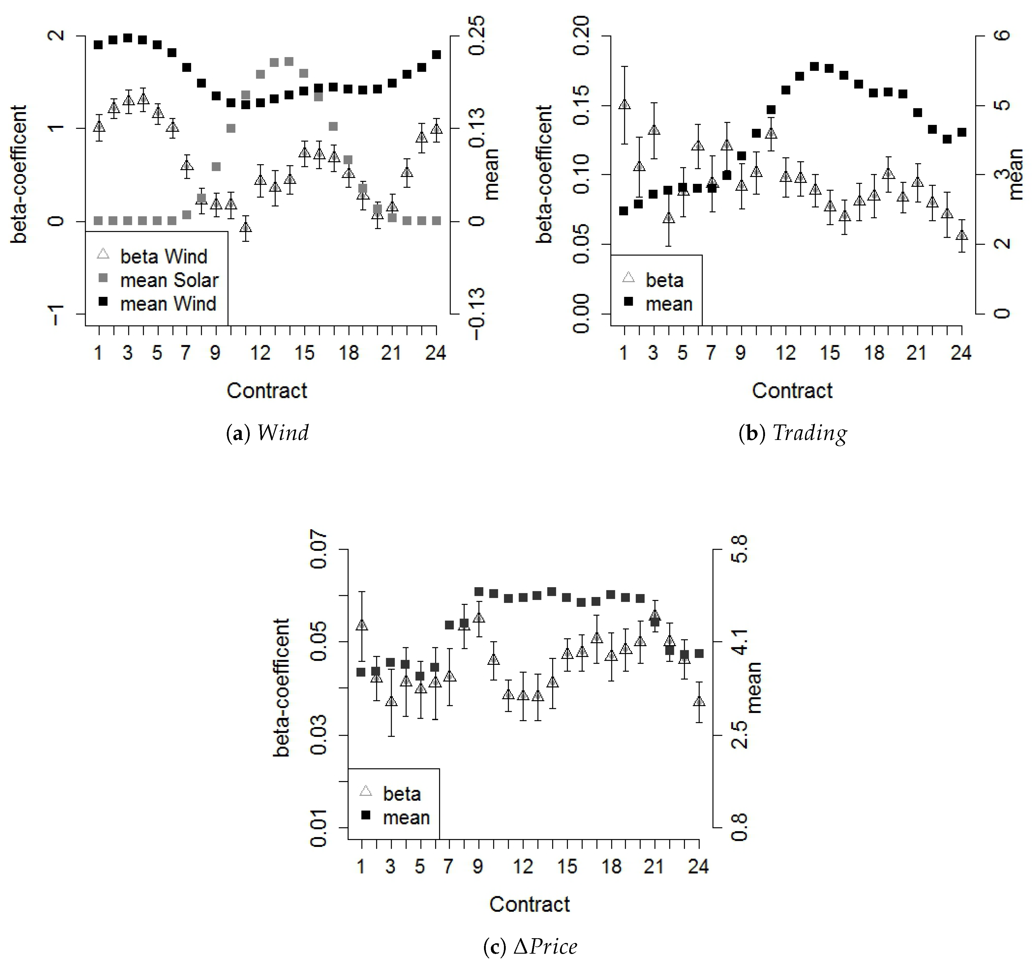
Figure 5 illustrates the coefficients for , , and , together with the respective mean values. For the share of wind energy (Figure 5a), the coefficients were highly significant for the contracts where the relative share of wind in the total mix was highest on average. This was accompanied by the highest adjusted values (especially in the morning hours). Apparently, the influence of solar energy leads to a respective reduction of the coefficients. There was a temporary increase in the coefficients when the relative wind share increased again and when the relative solar share decreased. Overall, the highest influence of wind energy coincides with the highest share of wind energy in the overall mix. For the trading volume (Figure 5b), the coefficients were at the fairly same level and were always significant. At peak load times, the traded volume of the continuous intraday market increased. This led to a reduction in the coefficients. For this reason, we conclude that the correlation of traded volume and dispersion is similar for all contracts. The same applies for the absolute difference between the average intraday price and the day-ahead price (Figure 5c). At peak load times, there are slightly higher average deviations between day-ahead auction prices and volume-weighted continuous intraday market prices as well as higher average dispersions. Nevertheless, the coefficients of the individual contracts are at a very similar level. The coefficients of solar energy are not illustrated since they are not significant even at the contract level and thus have no influence on price fluctuations. With regard to trading between foreign markets, the significance varies; no patterns of significance can be identified over the course of the day. This finding underpins the previous conclusion that this factor has the smallest explanatory power.
The analysis also helps to understand the coefficients of the fixed effects from Table 3, which were all positive except for the noon and afternoon contracts. Two different reasons partially account for the positive coefficients. The first reason is that, on average, these contracts are exposed to different price fluctuations than the 11 h–12 h reference contract. The second reason is that the explanatory variables have different levels at different points in time. For example, the average trading volume is higher for the peak contracts than for the off-peak contracts. Similar observations can be made for other variables. This is compensated by the positive coefficients. For the contracts with negative coefficients, only the second reason applies, since the mean price fluctuations are fairly close to each other. The negative coefficients arise from the fact that the variables with the highest explanatory power for these contracts are always higher than those of the reference contract (see also Figure 5). This is compensated by the negative coefficients.
5. Peak Trading and Volatility Forecasts
5.1. External Drivers of Price Fluctuations
We documented in Section 3.2 that a major part of the continuous intraday trading happens in the last hour before maturity. For this reason, the price dispersion during this period is the most relevant metric for many traders. We therefore took a closer look at price fluctuations during this peak trading time. The approach was analogous to Equation (7) in Section 4.1, where the trading-related variables , and refer only to the last hour before maturity and not to the entire period. The regression results, separately for the five measures, are given in Table 7.
The results of the regression are very similar to the results of the total price fluctuations. The interpretations are also analogous. Again, the four variables already identified, the relative share of wind energy, the trading volume, the amount of trading with foreign markets, and the absolute price difference between intraday and day-ahead market, turn out to be variables with explanatory power, with again having the least impact. For the other significant variables, the remarks from Section 4.1 apply analogously. Interestingly, the quality of the regressions, measured by the adjusted , was lower for all measures than for the regression for total price fluctuations. To a great extent, this can be explained by the variable. With the shortened time period, this price difference contains less information, as forecasts become more accurate when the delivery hour approaches. In addition, the importance of the day-ahead price decreased during the course of intraday trading: due to information received in the meantime, another reference price may already have been established, and trading activities may fluctuate around this price. Accordingly, price fluctuations in this period result more often from active trading than from forecast adjustments, and, as a result, the correlation of and price fluctuations decrease.
5.2. Forecast Indicators
While the previous analyses referred to the ex-post perspective, for a trader, it would be more interesting to have information about expected price fluctuations beforehand. In this section, we analyze to what extent forecast indicators for price fluctuations can be determined. The analysis focuses on the final (peak) trading hour, as more than 40% of the total volume is traded within this hour. Traders who want to settle their positions or conduct other trading strategies might want to know the extent of price fluctuations they have to consider in this peak trading hour.
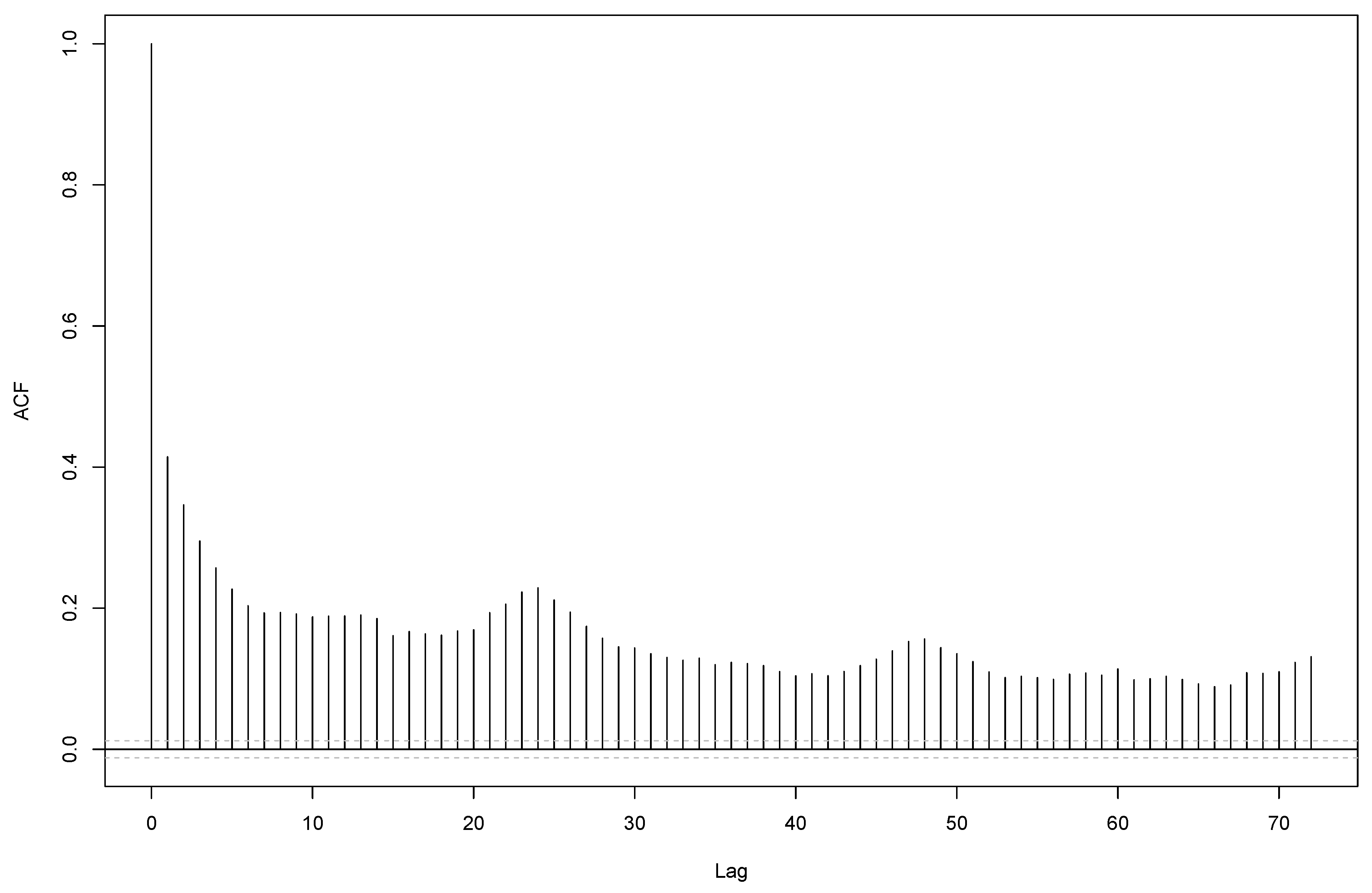
Price fluctuations throughout the day exhibit a timely structure. For the measure , the correlation between the dispersion of the last hour and the dispersion of the elapsed time amounts to . What is more, the price fluctuations during the final trading hour of contract h are correlated with the fluctuations during the final trading hour of the previously expired contract . This observation is in line with [20,21], who found similar results for the prices and price changes of 15-min contracts. Figure 6 illustrates these correlations for the measure .
The correlation between a contract h and the contract was most pronounced. However, there were also correlations between price fluctuations of contracts with larger time lags. For a time lag of 24 h, a temporary increase is actually evident, as this lag represents the same contract on the previous day. Thus, when it comes to peak trading during the last hour of a contract’s life, traders can use the information in the price history of the contract and furthermore of the previously expired contracts to forecast volatility and dispersion for the final hour. A forecasting regression combines information of the price time series (lagged realizations of the fluctuation measure) with external drivers that are known when the final trading hour starts. These variables are:
- the realized fluctuation measure of the specific contract during the elapsed time of trading ;
- lagged fluctuation measures for the contracts expired in the previous hours ;
- lagged fluctuation measures for the same hourly contract of the previous day ;
- the relative forecasted wind energy share of the forecasted total consumption
- the absolute (unsigned) difference between the last intraday price obtained immediately before the start of the last hour and the day-ahead price ;
- the absolute (unsigned) difference between the volume-weighted average intraday price obtained during the elapsed time of trading and the day-ahead price ;
- the traded volume during the elapsed time of trading ;
- the relative share of the total volume traded between Germany and a foreign country during the elapsed time of trading ;
- fixed effects for contracts, day, season, year, daylight saving time, and the possibility of later control zone trading.
The results of the forecasting regressions, separately for the five fluctuation measures, are given in Panel A of Table 8.
The explanatory power is highest for the absolute volatility with an adjusted of 0.479. Thus, half of the variance of this measure can be predicted beforehand. The values for the dispersion measures were considerably lower but still fairly large with values between 0.328 () and 0.201 ().
Regarding the explanatory variables, the results were quite similar for all measures. The price fluctuations of the observed contract are correlated with the lagged price fluctuations of the previous contracts. Consequently, high price fluctuations of previous contracts, as well as high price fluctuations of the same contract on the previous day and a week ago, indicate high price fluctuations of the observed contract. The price fluctuations of the contract that matured immediately before the observed contract have the highest explanatory power, which is also evident by Figure 6. Besides the price fluctuations of previous contracts, the realized price fluctuations of the same contract during the elapsed time of trading are also highly significant.
Furthermore, the price difference to the day-ahead price and the forecasted wind energy share can be identified as additional forecast indicators, in line with the results from Section 5.1. With regard to the variable , the last price before the final hour is an estimator for the volume-weighted average price of this last hour. Due to the high correlation of and , no additional significant impact of the price information from the total elapsed time via can be measured. With regard to the wind forecast, although it refers more to the day-ahead market, it is highly correlated with the share of wind energy, which we identified as an important external driver of price fluctuations. The significance of the total trading volume and the trading with foreign markets was fluctuating and partially not present in the regression. These factors can therefore only be identified as forecast indicators to a limited extent.
The fairly high explanatory power of the regressions can have three sources: information from the price history (lagged variables), information from external variables, and fixed effects. To analyze the relative importance of theses sources, we ran three additional regressions, exclusively with one group of variables each. The results are given in Panel B of Table 8. For all measures of price fluctuation, the lagged volatility had the greatest explanatory power, while the fixed effects had the least (with one exception). About 90% of the explanatory power of the entire regression (Panel A) can be achieved by the lagged variables only. Thus, the importance of time series characteristics or trading-related variables clearly outweighs the external variables. [22] showed that price information of neighboring contracts increases the forecast accuracy for intraday prices as opposed to fundamental factors. Our results complement these findings with price fluctuations. For a trader on the continuous intraday market, the observations of the previous time series of the different contracts allow a fairly precise forecast of future price fluctuations.
6. Conclusions
Volatility or dispersion measures that take into account the special features of the continuous intraday electricity market are similarly well suited for measuring intraday price fluctuations. Differences result from the robustness and the fundamental construction of the measures. For comparison, we considered five different measures, including a volatility-like measure, dispersion measures, and range measures. Over all contracts we observed average price fluctuations of about three EUR per MWh (based on the volume-weighted standard deviation) per MWh of electricity and price ranges of about EUR 20 per MWh (based on the total range). There were small differences between measures that took into account each trade and measures that drop information, while differences in the volatility measure that partly maintains the temporal structure were slightly larger. Although there were only minor differences between the measures, these exist both at the level of variable selection and at the level of forecast quality, which should be considered if only one measure is chosen as in [4,23]. We consider the volume-weighted standard deviation to be a reasonable dispersion measure, as it includes the volume of a trade.
To identify drivers of price fluctuations for the total as well as the short-term duration, we performed several multilinear regressions. In addition to various seasonalities (hourly, daily, and quarterly), we identified four exogenous factors that are related to price fluctuations:
- The relative share of wind in the overall mix is positively correlated with price fluctuations.
- The volume traded on the continuous intraday market is positively correlated with price fluctuations.
- The absolute deviation between the day-ahead auction price and the volume-weighted average price of the intraday market is positively correlated with price fluctuations.
- The relative traded volume between the German and foreign markets is negatively correlated with price fluctuations.
Our findings on wind energy complement the existing literature that analyzed day-ahead prices or volume-weighted intraday prices, e.g., [7,9] for the individual contracts of the continuous intraday market. Analogous to [2], we observed a higher influence of wind energy, especially for the off-peak contracts, but we cannot confirm their findings regarding solar energy on the contract level. Market states and trading behavior were identified by [11] as reasons for the differences between day-ahead prices and intraday prices. Our findings regarding the variables and confirm these results. Thus, changes in market fundamentals are also associated with greater price fluctuations. The influence of the variable is consistent with the thoughts of [23,25]. So far, the influence of this variable is relatively small, but considering the constantly changing market and projects to create a Europe-wide intraday market, its relevance could increase. The importance of the identified variables differs at the contract level. In all cases, the price difference can be identified as the variable with the greatest explanatory power for price fluctuations, whereas the relative traded volume between the German and foreign markets had the least explanatory power.
Nearly half of the intraday volume is traded during the last hour of each contract, similar to the Spanish intraday market (see [29]). We were the first to focus on forecasting price fluctuations at the contract level of the continuous intraday market, after [3] were already forecasting price fluctuations of average prices on the intraday market. Traders can use our results to forecast volatility and dispersion with information available when this final trading hour starts. Besides external drivers, we showed that characteristics of the (cross-sectional) time series of contracts can be used as forecasting variables. This complements the findings of [20,21], who found a similar correlation for 15-min contracts on prices. Because of (auto-)correlations, realized price fluctuations of previously expired contracts as well as fluctuations during the elapsed trading time of the contract itself have an explanatory power for price fluctuations during the (final) peak trading hour. We showed that trading-related variables play a more important role than fundamental factors in forecasting price fluctuation. This finding for forecasts on price fluctuations at the contract level also supplements previous findings on prices (e.g., [22]).
The impact of intraday updated forecasts on the prices of 15-min contracts in the intraday market was found by [4,21]. In our research, this kind of data was missing. As a result, the intraday-updated forecast errors were only indirectly included in the price difference variable. A topic for further investigation would be the inclusion of intraday updated forecasts. Under this aspect, the influence of renewable energies and forecasting errors should be examined more specifically.
Author Contributions
Conceptualization, R.B. and M.N.; methodology, R.B. and M.N.; software, M.N.; validation, R.B. and M.N.; formal analysis, M.N.; investigation, R.B. and M.N.; data curation, M.N.; writing—original draft preparation, R.B. and M.N.; writing—review & editing, R.B. and M.N.; visualization, M.N. All authors have read and agreed to the published version of the manuscript.
Funding
This research received no external funding.
Data Availability Statement
The data sets from the German Federal Network Agency are available online at smard.de, accessed on 7 November 2021.
Acknowledgments
We thank participants of the 26th Annual Meeting of the German Finance Association (DGF), of the 6th European Conference on Data Analysis (ECDA), and of the Working Group on Financial Management and Financial Institutions of the German Association of Operational Research (GOR AG FIFI) for valuable comments and suggestions.
Conflicts of Interest
The authors declare no conflict of interest.
References
- Paschen, M. Dynamic analysis of the German day-ahead electricity spot market. Energy Econ. 2016, 59, 118–128. [Google Scholar] [CrossRef] [Green Version]
- Rintamäki, T.; Siddiqui, A.S.; Salo, A. Does renewable energy generation decrease the volatility of electricity prices? An analysis of Denmark and Germany. Energy Econ. 2017, 62, 270–282. [Google Scholar] [CrossRef] [Green Version]
- Ciarreta, A.; Muniain, P.; Zarraga, A. Modeling and forecasting realized volatility in German-Austrian continuous intraday electricity prices. J. Forecast. 2017, 36, 680–690. [Google Scholar] [CrossRef]
- Kiesel, R.; Paraschiv, F. Econometric analysis of 15-minute intraday electricity price. Energy Econ. 2017, 64, 77–90. [Google Scholar] [CrossRef] [Green Version]
- Blanco, M.I. The economics of wind energy. Renew. Sustain. Energy Rev. 2009, 13, 1372–1382. [Google Scholar] [CrossRef]
- Nicolosi, M.; Fürsch, M. The impact of an increasing share of RES-E on the conventional power Market: The example of Germany. Z. Energ. 2009, 3, 246–254. [Google Scholar] [CrossRef]
- Ketterer, J. The impact of wind power generation on the electricity price in Germany. Energy Econ. 2014, 44, 270–280. [Google Scholar] [CrossRef] [Green Version]
- Benhmad, F.; Percebois, J. Wind power feed-in impact on electricity prices in Germany 2009–2013. Eur. J. Comp. Econ. 2016, 13, 81–96. [Google Scholar]
- Pape, C. The impact of intraday markets on the market value of flexibility—Decomposing effects on profile and the imbalance costs. Energy Econ. 2018, 76, 186–201. [Google Scholar] [CrossRef] [Green Version]
- Clò, S.; Cataldi, A.; Zoppoli, P. The merit-order effect in the Italian power market: The impact of solar and wind generation on national wholesale electricity prices. Energy Policy 2015, 77, 79–88. [Google Scholar] [CrossRef]
- Pape, C.; Hagemann, S.; Weber, C. Are fundamentals enough? Explaining price variations in the German day-ahead and intraday power market. Energy Econ. 2016, 54, 376–387. [Google Scholar] [CrossRef] [Green Version]
- Gürtler, M.; Paulsen, T. The effect of wind and solar power forecasts on day-ahead and intraday electricity prices in Germany. Energy Econ. 2018, 75, 150–162. [Google Scholar] [CrossRef]
- Maciejowska, K.; Uniejewski, B.; Serafin, T. PCA forecast averaging-Predicting day-ahead and intraday electricity prices. Energies 2020, 13, 3530. [Google Scholar] [CrossRef]
- Maciejowska, K.; Nitka, W.; Weron, T. Enhancing load, wind and solar generation for day-ahead forecasting of electricity prices. Energy Econ. 2021, 99, 105273. [Google Scholar] [CrossRef]
- Garnier, E.; Madlener, R. Balancing forecast errors in continuous-trade intraday markets. Energy Syst. 2015, 6, 362–388. [Google Scholar] [CrossRef]
- Kath, C.; Ziel, F. The value of forecasts: Quantifying the economic gains of accurate quarter-hourly electricity price forecasts. Energy Econ. 2018, 76, 411–423. [Google Scholar] [CrossRef] [Green Version]
- Märkle-Huß, J.; Feuerriegel, S.; Neumann, D. Contract durations in the electricity market: Causal impact of 15 min trading on the EPEX SPOT market. Energy Econ. 2018, 69, 367–378. [Google Scholar] [CrossRef] [Green Version]
- Uniejewski, B.; Marcjasz, G.; Weron, R. Understanding intraday electricity markets: Variable selection and very short-term price forecasting using LASSO. Int. J. Forecast. 2019, 35, 1533–1547. [Google Scholar] [CrossRef] [Green Version]
- Kulakov, S.; Ziel, F. The Impact of Renewable Energy Forecasts on Intraday Electricity Prices. Econ. Energy Environ. Policy 2021, 10. [Google Scholar] [CrossRef]
- Kremer, M.; Kiesel, R.; Paraschiv, F. Intraday electricity pricing of night contracts. Energies 2020, 13, 4501. [Google Scholar] [CrossRef]
- Kremer, M.; Kiesel, R.; Paraschiv, F. An econometric model for intraday electricity trading. Philos. Trans. R. Soc. A 2021, 379, 20190624. [Google Scholar] [CrossRef]
- Janke, T.; Steinke, F. Forecasting the price distribution of continuous intraday electricity trading. Energies 2019, 12, 4262. [Google Scholar] [CrossRef] [Green Version]
- Kath, C. Modeling intraday markets under the new advances of the cross-border intraday project (XBID): Evidence from the German intraday market. Energies 2019, 12, 4339. [Google Scholar] [CrossRef] [Green Version]
- Narajewski, M.; Ziel, F. Econometric modelling and forecasting of intraday electricity prices. J. Commod. Mark. 2020, 19, 100107. [Google Scholar] [CrossRef] [Green Version]
- Narajewski, M.; Ziel, F. Ensemble Forecasting for Intraday Electricity Prices: Simulating Trajectories. Appl. Energy 2020, 279, 115801. [Google Scholar] [CrossRef]
- Glas, S.; Kiesel, R.; Kolkmann, S.; Kremer, M.; Graf von Luckner, N.; Ostmeier, L.; Weber, C. Intraday renewable electricity trading: Advanced modeling and numerical optimal control. J. Math. Ind. 2020, 10, 3. [Google Scholar] [CrossRef]
- Kramer, A.; Kiesel, R. Exogenous factors for order arrivals on the intraday electricity mar et. Energy Econ. 2021, 97, 105186. [Google Scholar] [CrossRef]
- Girish, G.P.; Vijayalakshmi, S. Determinants of electricity price in competitive power market. Int. J. Bus. Manag. 2013, 8, 70–75. [Google Scholar]
- Scharff, R.; Amelin, M. Trading behaviour on the continuous intraday market Elbas. Energy Policy 2016, 88, 544–557. [Google Scholar] [CrossRef]
- Garman, M.B.; Klass, M.J. On the estimation of security price volatilities from historic data. J. Bus. 1980, 53, 67–78. [Google Scholar] [CrossRef]
- Mugele, C.; Rachev, S.T.; Trück, S. Stable modeling on different European power markets. Invest. Manag. Financ. Innov. 2005, 3, 65–85. [Google Scholar]
- Gianfreda, A. Volatility and volume effects in European electricity spot markets. Econ. Notes 2010, 39, 47–63. [Google Scholar] [CrossRef]
- Janczura, J.; Trück, S.; Weron, R.; Wolff, R. Identifying spikes and seasonal components in electricity spot price data: A guide to robust modeling. Energy Econ. 2013, 38, 96–110. [Google Scholar] [CrossRef] [Green Version]
- Afanasyev, D.O.; Fedorova, E.A. On the impact of outlier filtering on the electricity price forecasting accuracy. Appl. Energy 2019, 236, 196–210. [Google Scholar] [CrossRef]
- Newey, W.K.; West, K.D. Hypothesis testing with efficient method of moments estimation. Int. Econ. Rev. 1987, 28, 777–787. [Google Scholar] [CrossRef]
- Zachmann, G. Electricity wholesale market prices in Europe: Convergence? Energy Econ. 2008, 30, 1659–1671. [Google Scholar] [CrossRef]
- Weber, C. Adequate intraday market design to enable the integration of wind energy into the European power systems. Energy Policy 2010, 38, 3155–3163. [Google Scholar] [CrossRef]
Figure 1.
Typical structure of a trading day on EPEX SPOT. The day-ahead auction is at 12 p.m. (noon). Trading for hourly contracts on the continuous intraday market starts at 3 p.m. and is possible until 5 min before delivery. Until June 2017, trading on the continuous intraday market was possible only up to 30 min before delivery. Afterwards, trading was possible within a control zone until 5 min before delivery.

Figure 2.
Selected realized price development of the 00h–01h contract on 23 September 2018 with remaining maturity of the continuous intraday market. The figure illustrates the differences between a classic stock market and the continuous intraday market for electricity. There are large price movements from about EUR 20 to 80 per MWh within the few hours of trading. Furthermore, trades are unevenly distributed and cluster at the end of the period.

Figure 3.
Relative trading volume of the continuous intraday market per hour before maturity (up to 30 min before delivery). The figure illustrates that trading volume increases sharply with decreasing time to maturity.
Figure 3.
Relative trading volume of the continuous intraday market per hour before maturity (up to 30 min before delivery). The figure illustrates that trading volume increases sharply with decreasing time to maturity.

Figure 4.
Histograms of all realized prices (subfigure (a)) and the total five price fluctuation measures (subfigures (b–f)). Extreme values at the tails of the distributions were omitted to provide clarity.
Figure 4.
Histograms of all realized prices (subfigure (a)) and the total five price fluctuation measures (subfigures (b–f)). Extreme values at the tails of the distributions were omitted to provide clarity.


Figure 5.
Regression -coefficients (left axis) for the volume-weighted average standard deviation as the dependent variable, with standard errors, plotted against the corresponding mean (right axis) of the variables separately for the individual hourly contracts. Subfigure (a) shows as the relative wind share of the total consumption (together with the relative solar share of the total consumption ). Subfigure (b) shows as the traded volume of the intraday market in GWh, and Subfigure (c) shows as the absolute price difference of the day-ahead auction price and the volume-weighted average price of the intraday market. Significant influence of coincides with the highest share of wind energy in the overall mix. and were always significant regardless of fluctuating averages.

Figure 6.
Autocorrelations of the dispersion measure , the volume-weighted average standard deviation for the final trading hour. Especially for small lags, the correlation is pronounced. A correlation with the price fluctuations of the same hourly contract on the previous day (lag 24) can also be observed.


Table 1.
Descriptive statistics and correlations between the five fluctuation measures. Panel A covers all data and Panel B only the final trading hour of each contract. is the standard deviation of the price differences of consecutive trades. is the standard deviation, the volume-weighted average standard deviation, the range, and the interquartile range of all prices for a single contract. All figures of the descriptive statistics for the measures are given in EUR per MWh.
| Panel A: Total Price Fluctuations | Panel B: Last Trading Hour | ||||||||||
|---|---|---|---|---|---|---|---|---|---|---|---|
| Transactions | 13.6 millions | 6.2 millions | |||||||||
| Volume | 102 TWh | 44 TWh | |||||||||
| 1% | 0.293 | 0.872 | 0.854 | 4.900 | 0.900 | 0.245 | 0.606 | 0.594 | 2.800 | 0.600 | |
| 25% | 0.527 | 1.862 | 1.854 | 10.25 | 2.200 | 0.482 | 1.447 | 1.434 | 6.500 | 1.800 | |
| Median | 0.706 | 2.682 | 2.681 | 14.40 | 3.300 | 0.667 | 2.155 | 2.138 | 9.500 | 2.900 | |
| Mean | 0.881 | 3.409 | 3.409 | 18.49 | 4.397 | 0.830 | 2.804 | 2.778 | 12.21 | 3.941 | |
| 75% | 0.987 | 3.967 | 3.956 | 21.19 | 5.200 | 0.943 | 3.304 | 3.278 | 14.00 | 4.800 | |
| 99% | 3.393 | 14.88 | 14.84 | 79.58 | 19.80 | 3.241 | 12.16 | 12.23 | 53.10 | 18.12 | |
| SD | 1.310 | 3.215 | 3.682 | 21.88 | 4.367 | 1.148 | 3.007 | 2.930 | 13.59 | 4.250 | |
| Skewness | 38.78 | 9.325 | 28.27 | 21.51 | 7.235 | 40.19 | 14.15 | 14.10 | 15.25 | 8.857 | |
| Kurtosis | 2087 | 193.9 | 1989 | 826.6 | 105.0 | 2493 | 443.0 | 453.8 | 444.9 | 183.2 | |
| 1 | - | - | - | - | 1 | - | - | - | - | ||
| 0.542 | 1 | - | - | - | 0.653 | 1 | - | - | - | ||
| 0.527 | 0.875 | 1 | - | - | 0.592 | 0.982 | 1 | - | - | ||
| 0.872 | 0.810 | 0.754 | 1 | - | 0.786 | 0.923 | 0.887 | 1 | - | ||
| 0.256 | 0.843 | 0.739 | 0.516 | 1 | 0.364 | 0.861 | 0.883 | 0.698 | 1 | ||
Table 2.
Descriptive statistics of the explanatory variables. is the relative solar share of the total consumption, and is the relative solar forecast error of the total consumption. and are analogously defined as the relative wind share and the relative wind forecast error of the total consumption. is the volume of the total consumption in TWh, is the unsigned relative excess generation over consumption in Germany, is the traded volume of the intraday market in GWh, is the relative share of the volume (buy and sell) traded between Germany and a foreign country and the total traded volume of the intraday market, and is the absolute price difference of the day-ahead auction price and the volume-weighted average intraday price.
| Min | 0.0000 | 0.00000 | 0.002 | 0.0000 | 0.031 | 0.000 | 0.272 | 0.000 | 0.000 |
| 25% | 0.0000 | 0.00000 | 0.077 | 0.0054 | 0.048 | 0.044 | 2.715 | 0.075 | 1.437 |
| Median | 0.0023 | 0.00030 | 0.154 | 0.0124 | 0.056 | 0.087 | 3.709 | 0.192 | 3.101 |
| Mean | 0.0704 | 0.00525 | 0.191 | 0.0180 | 0.056 | 0.105 | 3.928 | 0.203 | 4.397 |
| 75% | 0.1097 | 0.00639 | 0.270 | 0.0247 | 0.065 | 0.149 | 4.893 | 0.312 | 5.660 |
| Max | 0.5837 | 0.09744 | 0.848 | 0.2829 | 0.079 | 0.536 | 14.31 | 0.718 | 111.3 |
| SD | 0.1090 | 0.00979 | 0.147 | 0.0182 | 0.010 | 0.079 | 1.625 | 0.144 | 5.057 |
Table 3.
Regression results for the five measures for the total price fluctuations. is the standard deviation of the price differences consecutive trades, is the standard deviation, is the volume-weighted average standard deviation, is the range, and is the interquartile range of all observable prices. is the relative solar share of the total consumption, and is the relative solar forecast error of the total consumption. and are analogously defined as the relative wind share and the relative wind forecast error of the total consumption. is the volume of the total consumption in TWh, is the unsigned relative excess generation over consumption in Germany, is the traded volume of the intraday market in GWh, is the relative share of the volume (buy and sell) traded between Germany and a foreign country and the total traded volume of the intraday market, and is the absolute price difference of the day-ahead auction price and the volume-weighted average intraday price. The successive variables represent fixed effects for hour, day, season, year, summer time, and late trading within a control zone. RMSE is the root mean squared error, and MAE is the mean absolute error. The asterisks denote the significance level with *** = 0.1%, ** = 1%, and * = 5%.
| −0.549 *** | 0.494 *** | 0.489 *** | 2.021 *** | 0.737 *** | |
| 0.219 * | 0.242 * | 0.321 ** | 0.142 | 0.375 ** | |
| −0.170 | −0.560 | −0.555 | −0.175 | −1.293 | |
| 0.571 *** | 0.719 *** | 0.767 *** | 0.716 *** | 0.831 *** | |
| −1.183 *** | −1.400 *** | −1.596 *** | −1.044 *** | −1.890 *** | |
| 1.422 | 0.560 | 0.357 | 3.940 * | −0.226 | |
| 0.159 | −0.220 | −0.303 * | −0.023 | −0.333 * | |
| −0.012 * | 0.085 *** | 0.088 *** | 0.076 *** | 0.098 *** | |
| −0.124 ** | −0.279 *** | −0.349 *** | −0.138 ** | −0.503 *** | |
| 0.033 *** | 0.049 *** | 0.047 *** | 0.046 *** | 0.046 *** | |
| 0.276 *** | 0.191 *** | 0.203 *** | 0.170 *** | 0.181 *** | |
| 0.244 *** | 0.151 *** | 0.172 *** | 0.144 ** | 0.151 ** | |
| 0.243 *** | 0.135 ** | 0.146 ** | 0.134 ** | 0.131 * | |
| 0.269 *** | 0.158 *** | 0.171 *** | 0.159 *** | 0.145 ** | |
| 0.301 *** | 0.158 *** | 0.168 *** | 0.163 *** | 0.128 ** | |
| 0.405 *** | 0.237 *** | 0.257 *** | 0.237 *** | 0.241 *** | |
| 0.454 *** | 0.334 *** | 0.347 *** | 0.312 *** | 0.332 *** | |
| 0.434 *** | 0.357 *** | 0.395 *** | 0.326 *** | 0.379 *** | |
| 0.279 *** | 0.271 *** | 0.289 *** | 0.219 *** | 0.313 *** | |
| 0.143 *** | 0.147 *** | 0.154 *** | 0.113 *** | 0.160 *** | |
| 0.024 * | 0.036 ** | 0.039 ** | 0.012 | 0.030 | |
| −0.051 *** | −0.038 ** | −0.041 ** | −0.040 ** | −0.029 | |
| −0.066 *** | −0.068 *** | −0.066 *** | −0.071 *** | −0.056 ** | |
| −0.029 * | −0.046 ** | −0.044 * | −0.029 | −0.051 * | |
| 0.002 | 0.006 | 0.017 | 0.006 | 0.014 | |
| 0.024 | 0.016 | 0.029 | 0.022 | 0.020 | |
| 0.090 *** | 0.085 *** | 0.094 *** | 0.079 *** | 0.078 ** | |
| 0.159 *** | 0.122 *** | 0.140 *** | 0.143 *** | 0.126 *** | |
| 0.198 *** | 0.152 *** | 0.175 *** | 0.163 *** | 0.152 *** | |
| 0.202 *** | 0.160 *** | 0.181 *** | 0.170 *** | 0.167 *** | |
| 0.205 *** | 0.151 *** | 0.168 *** | 0.155 *** | 0.149 *** | |
| 0.272 *** | 0.221 *** | 0.243 *** | 0.227 *** | 0.207 *** | |
| 0.598 *** | 0.240 *** | 0.376 *** | 0.397 *** | 0.281 *** | |
| −0.117 *** | −0.095 *** | −0.094 *** | −0.109 *** | −0.095 ** | |
| −0.147 *** | −0.131 *** | −0.128 *** | −0.129 *** | −0.132 *** | |
| −0.160 *** | −0.130 *** | −0.131 *** | −0.146 *** | −0.130 *** | |
| −0.206 *** | −0.152 *** | −0.149 *** | −0.181 *** | −0.145 *** | |
| −0.190 *** | −0.164 *** | −0.162 *** | −0.181 *** | −0.162 *** | |
| −0.118 *** | −0.093 *** | −0.095 *** | −0.101 *** | −0.093 *** | |
| −0.084 * | −0.070 * | −0.073 * | −0.031 | −0.104 ** | |
| −0.104 * | −0.023 | −0.036 | 0.005 | −0.096 * | |
| 0.066 | 0.114 *** | 0.118 *** | 0.164 *** | 0.086 ** | |
| 2015 | 0.162 ** | −0.035 | −0.023 | −0.168 ** | 0.001 |
| 2016 | −0.008 | −0.151 *** | −0.132 ** | −0.205 *** | −0.097 * |
| 2017 | −0.011 | −0.078** | −0.079 ** | −0.137 *** | −0.045 |
| −0.107 ** | −0.035 | −0.045 | −0.071 * | −0.029 | |
| 0.006 | −0.060 | −0.056 | −0.013 | −0.047 | |
| adj. | 0.436 | 0.425 | 0.425 | 0.447 | 0.357 |
| 0.364 | 0.430 | 0.434 | 0.412 | 0.523 | |
| 0.279 | 0.341 | 0.344 | 0.318 | 0.415 | |
| # Observations | 24,893 | 24,906 | 24,913 | 24,904 | 24,926 |
Table 4.
Correlations between the explanatory variables and the volume-weighted average standard deviation . is the relative solar share of the total consumption, and is the relative solar forecast error of the total consumption. and are analogously defined as the relative wind share and the relative wind forecast error of the total consumption. is the volume of the total consumption in TWh, is the unsigned relative excess generation over consumption in Germany, is the traded volume of the intraday market in GWh, is the relative share of the volume (buy and sell) traded between Germany and a foreign country and the total traded volume of the intraday market, and is the absolute price difference of the day-ahead auction price and the volume-weighted average intraday price.
| 1 | - | - | - | - | - | - | - | - | |
| 0.588 | 1 | - | - | - | - | - | - | - | |
| −0.229 | −0.128 | 1 | - | - | - | - | - | - | |
| −0.100 | −0.055 | 0.367 | 1 | - | - | - | - | - | |
| 0.267 | 0.241 | −0.126 | −0.066 | 1 | - | - | - | - | |
| 0.029 | −0.026 | 0.441 | 0.157 | −0.486 | 1 | - | - | - | |
| 0.343 | 0.386 | 0.033 | 0.160 | 0.494 | −0.287 | 1 | - | - | |
| −0.020 | −0.051 | −0.361 | −0.123 | −0.223 | −0.299 | 0.103 | 1 | - | |
| 0.007 | 0.089 | 0.286 | 0.217 | 0.084 | 0.114 | 0.273 | −0.134 | 1 | |
| −0.062 | 0.021 | 0.364 | 0.182 | 0.107 | 0.093 | 0.269 | −0.193 | 0.550 |
Table 5.
Regression results for the volume-weighted average standard deviation as dependent variable for different models. Panel A contains the coefficients of univariate regressions with additional fixed effects for contracts, day, season, year, daylight saving time, and the possibility of control zone trading later. Panel B contains the coefficients of different multivariate regression designs. is the relative solar share of the total consumption, is the relative wind share of the total consumption, and is the relative solar forecast error of the total consumption. is the unsigned relative excess generation over consumption in Germany, is the traded volume of the intraday market in GWh, is the relative share of the volume (buy and sell) traded between Germany and a foreign country and the total traded volume of the intraday market, and is the absolute price difference of the day-ahead auction price and the volume-weighted average intraday price. FE denotes fixed effects. RMSE is the root mean squared error and MAE is the mean absolute error. The asterisks denote the significance level with *** = 0.1% and ** = 1%.
| Panel A | Panel B | ||||||||||||
|---|---|---|---|---|---|---|---|---|---|---|---|---|---|
| −0.107 | - | - | - | - | - | - | - | 0.268 ** | - | - | - | ||
| (0.148) | (0.093) | ||||||||||||
| - | 1.361 *** | - | - | - | - | - | 0.908 *** | 0.778 *** | 0.785 *** | 0.833 *** | 0.792 *** | 0.653 *** | |
| (0.086) | (0.056) | (0.053) | (0.062) | (0.061) | (0.064) | (0.065) | |||||||
| - | - | 4.655 *** | - | - | - | - | - | - | - | −1.486 *** | - | - | |
| (0.457) | - | (0.323) | |||||||||||
| - | - | - | 0.982 *** | - | - | - | - | - | - | - | −0.072 | - | |
| (0.193) | (0.108) | ||||||||||||
| - | - | - | - | 0.155 *** | - | - | 0.049 *** | 0.072 *** | 0.074 *** | 0.076 *** | 0.072 *** | 0.083 *** | |
| (0.006) | (0.004) | (0.005) | (0.005) | (0.005) | (0.005) | (0.005) | |||||||
| - | - | - | - | - | −0.565 *** | - | - | - | - | - | - | −0.335 *** | |
| (0.075) | (0.046) | ||||||||||||
| - | - | - | - | - | - | 0.059 *** | 0.052 *** | 0.048 *** | 0.047 *** | 0.048 *** | 0.048 *** | 0.047 *** | |
| (0.003) | (0.003) | (0.003) | (0.003) | (0.003) | (0.003) | (0.003) | |||||||
| FE | yes | yes | yes | yes | yes | yes | yes | no | yes | yes | yes | yes | yes |
| Adj. | 0.125 | 0.224 | 0.145 | 0.136 | 0.220 | 0.139 | 0.363 | 0.367 | 0.418 | 0.419 | 0.420 | 0.418 | 0.422 |
| 0.536 | 0.505 | 0.530 | 0.533 | 0.506 | 0.532 | 0.458 | 0.456 | 0.437 | 0.437 | 0.436 | 0.437 | 0.436 | |
| 0.421 | 0.395 | 0.416 | 0.419 | 0.397 | 0.418 | 0.361 | 0.361 | 0.346 | 0.346 | 0.346 | 0.346 | 0.345 | |
Table 6.
Results for the volume-weighted average standard deviation as the dependent variable, separated by season and day. Panel A contains the descriptive statistics, and Panel B contains the regression results. is the relative wind share of the total consumption, is the traded volume of the intraday market in GWh, is the relative share of the volume (buy and sell) traded between Germany and a foreign country and the total traded volume of the intraday market, and is the absolute price difference of the day-ahead auction price and the volume-weighted average intraday price. RMSE is the root mean squared error, and MAE is the mean absolute error. The asterisks denote the significance level with *** = 0.1%.
| : | Workday | Sunday/Holiday | Spring | Summer | Autumn | Winter |
|---|---|---|---|---|---|---|
| Panel A: Descriptive Statistics | ||||||
| 1% | 0.845 | 0.920 | 0.843 | 0.753 | 0.968 | 0.975 |
| 25% | 1.813 | 2.126 | 1.723 | 1.616 | 2.157 | 2.096 |
| Median | 2.603 | 3.125 | 2.443 | 2.277 | 3.112 | 3.034 |
| Mean | 3.279 | 4.083 | 3.074 | 2.892 | 3.772 | 3.936 |
| 75% | 3.835 | 4.713 | 3.487 | 3.368 | 4.486 | 4.544 |
| 99% | 13.60 | 18.44 | 13.98 | 11.38 | 14.14 | 18.50 |
| SD | 3.059 | 5.894 | 4.687 | 2.877 | 2.902 | 3.837 |
| Skewness | 10.45 | 34.74 | 44.76 | 15.90 | 5.945 | 8.119 |
| Kurtosis | 247.9 | 1762 | 2858 | 527.1 | 79.48 | 136.6 |
| Panel B: Regression Results | ||||||
| 0.660 *** | 1.086 *** | 0.788 *** | 0.958 *** | 0.678 *** | 0.611 *** | |
| (0.064) | (0.123) | (0.128) | (0.130) | (0.095) | (0.116) | |
| 0.083 *** | 0.098 *** | 0.087 *** | 0.093 *** | 0.095 *** | 0.076 *** | |
| (0.006) | (0.011) | (0.009) | (0.011) | (0.010) | (0.010) | |
| −0.263 *** | −0.464 *** | −0.288 *** | −0.264 *** | −0.138 | −0.464 *** | |
| (0.055) | (0.103) | (0.077) | (0.076) | (0.093) | (0.100) | |
| 0.054 *** | 0.031 *** | 0.045 *** | 0.061 *** | 0.049 *** | 0.042 *** | |
| (0.002) | (0.003) | (0.008) | (0.004) | (0.003) | (0.003) | |
| Adj. | 0.418 | 0.454 | 0.386 | 0.398 | 0.401 | 0.424 |
| 0.431 | 0.441 | 0.421 | 0.433 | 0.428 | 0.443 | |
| 0.341 | 0.350 | 0.332 | 0.343 | 0.341 | 0.348 | |
| # Observations | 21,607 | 4160 | 6529 | 6643 | 6262 | 6331 |
Table 7.
Regression results for the five price fluctuations measures for the last trading hour. is the standard deviation of the price differences consecutive trades, is the standard deviation, is the volume-weighted average standard deviation, is the range, and is the interquartile range of all observable prices. is the relative solar share of the total consumption, and is the relative solar forecast error of the total consumption. and are analogously defined as the relative wind share and the relative wind forecast error of the total consumption. is the volume of the total consumption in TWh, is the unsigned relative excess generation over consumption in Germany, is the traded volume of the intraday market in GWh, is the relative share of the volume (buy and sell) traded between Germany and a foreign country and the total traded volume of the intraday market, and is the absolute price difference of the day-ahead auction price and the volume-weighted average intraday price. RMSE is the root mean squared error, and MAE is the mean absolute error. The asterisks denote the significance level with *** = 0.1%, ** = 1%, and * = 5%.
| −0.246 * | 0.536 *** | 0.523 *** | 2.004 *** | 0.878 *** | |
| (0.106) | (0.122) | (0.119) | (0.120) | (0.134) | |
| 0.112 | 0.115 | 0.106 | 0.092 | 0.091 | |
| (0.106) | (0.117) | (0.117) | (0.113) | (0.125) | |
| 0.822 | −1.436 | −1.576 * | −0.837 | −2.482 ** | |
| (0.679) | (0.788) | (0.785) | (0.761) | (0.859) | |
| 0.475 *** | 0.562 *** | 0.564 *** | 0.602 *** | 0.557 *** | |
| (0.069) | (0.077) | (0.075) | (0.076) | (0.075) | |
| −0.733 * | −1.298 *** | −1.342 *** | −1.081 ** | −1.449 *** | |
| (0.312) | (0.367) | (0.363) | (0.350) | (0.397) | |
| −5.417 *** | −4.208 * | −3.974 * | −3.837 * | −4.286 * | |
| (0.016) | (0.018) | (0.018) | (0.018) | (0.020) | |
| −0.198 | −0.372 ** | −0.374 ** | −0.367 ** | −0.377 ** | |
| (0.132) | (0.141) | (0.139) | (0.138) | (0.143) | |
| −0.015 | 0.234 *** | 0.235 *** | 0.240 *** | 0.239 *** | |
| (0.010) | (0.011) | (0.011) | (0.011) | (0.012) | |
| 0.040 | −0.192 *** | −0.279 *** | −0.092* | −0.551 *** | |
| (0.041) | (0.049) | (0.050) | (0.046) | (0.059) | |
| 0.029 *** | 0.031 *** | 0.031 *** | 0.030 *** | 0.032 *** | |
| (0.002) | (0.002) | (0.002) | (0.002) | (0.002) | |
| Fixed Effects | yes | yes | yes | yes | yes |
| Adj. | 0.363 | 0.276 | 0.273 | 0.307 | 0.222 |
| 0.434 | 0.549 | 0.551 | 0.510 | 0.671 | |
| 0.338 | 0.438 | 0.440 | 0.402 | 0.539 | |
| # Observations | 24,896 | 24,920 | 24,922 | 24,901 | 24,933 |
Table 8.
Results of the forecast regressions for the five measures (the standard deviation of the price differences consecutive trades), (the standard deviation of all trades for a contract), (the volume-weighted standard deviation of all trades for a contract), (the range of all trades for a contract), and (the interquartile range of all trades for a contract). Panel A shows the results of the full regression, and Panel B shows the adjusted of separate regressions, using exclusively the fixed effects, the external variables, and the lagged variables, respectively. , , , , are lagged fluctuations measures for the contracts expired in the previous hours, and is the realized fluctuation measure of the specific contract during the elapsed time of trading. is the traded volume during the elapsed time of trading, is the relative share of the total volume traded between Germany and a foreign country during the elapsed time of trading, is the absolute (unsigned) difference between the last intraday price obtained immediately before the start of the last hour and the day-ahead price, is the absolute (unsigned) difference between the volume-weighted average intraday price obtained during the elapsed time of trading and the day-ahead price, and is the relative forecasted wind energy share of the forecasted total consumption. RMSE is the root mean squared error, and MAE is the mean absolute error. The asterisks denote the significance level with *** = 0.1% and * = 5.0%.
| Panel A: Full Regression Results | |||||
| −0.322 *** | 0.263 *** | 0.271 *** | 0.766 *** | 0.509 *** | |
| (0.022) | (0.032) | (0.032) | (0.042) | (0.041) | |
| 0.291 *** | 0.192 *** | 0.187 *** | 0.229 *** | 0.132 *** | |
| (0.008) | (0.007) | (0.007) | (0.007) | (0.007) | |
| 0.119 *** | 0.102 *** | 0.104 *** | 0.117 *** | 0.082 *** | |
| (0.007) | (0.007) | (0.007) | (0.007) | (0.007) | |
| 0.074 *** | 0.068 *** | 0.068 *** | 0.082 *** | 0.067 *** | |
| (0.007) | (0.006) | (0.006) | (0.006) | (0.007) | |
| 0.069 *** | 0.060 *** | 0.062 *** | 0.066 *** | 0.050 *** | |
| (0.006) | (0.006) | (0.006) | (0.006) | (0.006) | |
| 0.038 *** | 0.030 *** | 0.029 *** | 0.035 *** | 0.024 *** | |
| (0.006) | (0.006) | (0.006) | (0.006) | (0.006) | |
| 0.121 *** | 0.159 *** | 0.142 *** | 0.103 *** | 0.110 *** | |
| (0.007) | (0.011) | (0.010) | (0.010) | (0.009) | |
| −0.007 * | 0.006 | 0.004 | 0.008 | 0.015** | |
| (0.003) | (0.004) | (0.005) | (0.004) | (0.006) | |
| 0.064 *** | 0.105 *** | 0.091 *** | 0.096 *** | 0.024 | |
| (0.017) | (0.024) | (0.025) | (0.023) | (0.029) | |
| 0.008 *** | 0.006 *** | 0.007 *** | 0.010 *** | 0.010 *** | |
| (0.001) | (0.001) | (0.001) | (0.001) | (0.002) | |
| −0.002 | 0.001 | 0.001 | −0.003 | 0.002 | |
| (0.001) | (0.002) | (0.002) | (0.002) | (0.002) | |
| 0.121 *** | 0.402 *** | 0.417 *** | 0.399 *** | 0.519 *** | |
| (0.024) | (0.035) | (0.035) | (0.033) | (0.047) | |
| Adj. | 0.479 | 0.285 | 0.278 | 0.328 | 0.201 |
| 0.365 | 0.516 | 0.521 | 0.475 | 0.654 | |
| 0.280 | 0.411 | 0.415 | 0.373 | 0.524 | |
| # Observations | 24,496 | 24,609 | 24,642 | 24,524 | 24,675 |
| Panel B: Adjusted of Separate Regressions | |||||
| FE | 0.213 | 0.076 | 0.074 | 0.090 | 0.061 |
| External | 0.183 | 0.155 | 0.154 | 0.175 | 0.122 |
| Lagged | 0.438 | 0.266 | 0.259 | 0.307 | 0.175 |
Publisher’s Note: MDPI stays neutral with regard to jurisdictional claims in published maps and institutional affiliations. |
© 2021 by the authors. Licensee MDPI, Basel, Switzerland. This article is an open access article distributed under the terms and conditions of the Creative Commons Attribution (CC BY) license (https://creativecommons.org/licenses/by/4.0/).
Share and Cite
MDPI and ACS Style
Baule, R.; Naumann, M. Volatility and Dispersion of Hourly Electricity Contracts on the German Continuous Intraday Market. Energies 2021, 14, 7531. https://doi.org/10.3390/en14227531
AMA Style
Baule R, Naumann M. Volatility and Dispersion of Hourly Electricity Contracts on the German Continuous Intraday Market. Energies. 2021; 14(22):7531. https://doi.org/10.3390/en14227531
Chicago/Turabian StyleBaule, Rainer, and Michael Naumann. 2021. "Volatility and Dispersion of Hourly Electricity Contracts on the German Continuous Intraday Market" Energies 14, no. 22: 7531. https://doi.org/10.3390/en14227531
Note that from the first issue of 2016, this journal uses article numbers instead of page numbers. See further details here.