Article

Balancing Energy Trilemma Using Hybrid Distributed Rooftop Solar PV (DRSP)/Battery/Diesel Microgrid: A Case Study in Gilutongan Island, Cordova, Cebu, Philippines

1
Center for Research in Energy Systems and Technologies and Engineering Graduate Program, University of San Carlos, Cebu City 6000, Philippines
2
Department of Electrical and Electronics Engineering, University of San Carlos, Cebu City 6000, Philippines
3
Department of Chemical Engineering, University of San Carlos, Cebu City 6000, Philippines
*
Author to whom correspondence should be addressed.
Energies 2021, 14(21), 7358; https://doi.org/10.3390/en14217358
Submission received: 28 September 2021 / Revised: 17 October 2021 / Accepted: 19 October 2021 / Published: 5 November 2021

Abstract

:
Design strategies for achieving reliable, affordable, and clean electricity are crucial for energy sustainability. Attaining it requires managing the three core factors (TCF) of the energy trilemma (ET) to increase reliability (energy equity), minimize the levelized cost of electricity (LCOE) (energy equity), and avoid potential CO2 emission (environmental sustainability) simultaneously. This paper aims to present a design strategy for the hybrid energy system microgrid (HESM) model, consisting of a distributed rooftop solar PV (DRSP), battery, and diesel-generator to meet the increasing demand while balancing the TCF of the ET. The design strategy was applied in a cluster of 11 households in Gilutongan Island, Cebu, Philippines, where there is no open land space for a solar PV microgrid system. This study used PVSyst and HOMER Pro software to perform the techno-enviro-economic (TEE) analysis to select all feasible system configurations (FSCs). To identify the optimal FSC, a scoring mechanism that considers the LCOE based on the 5% household electricity expense limit, the 5% unmet load fraction, and the renewable penetration fraction was used. Results show that the optimal system requires an average of 32.2% excess energy from DRSP to balance the TCF of the ET based on the energy demand considered. Thus, planning when energy demand increases is vital to map the next appropriate steps toward sustainable energy transition. Overall, the obtained results can support project developers and policymakers to make informed decisions in balancing the ET from various trade-offs of energy systems.

1. Introduction

According to the International Energy Agency’s 2019 report, significant progress is happening in energy access worldwide. From 1.2 billion in 2010 to 1 billion in 2016, it dropped to roughly 840 million people living without electricity access due to an increased deployment of off-grid technologies. However, the most significant challenge remains in connecting the poorest and hardest to reach households in the numerous remote areas globally and in Sub-Saharan Africa, where 573 million people still live in the dark [1].
In the Philippines, the National Electrification Administration (NEA) published a report that there are still 1,577,672 unserved consumers based on the potential customers of the 2015 Census [2]. Particularly in small off-grid islands (SOIs), the remoteness, low energy demand, and lower population often make grid extension not viable [3]. Furthermore, most SOIs in the Philippines, not electrified by any power providers, are powered primarily by diesel generators (DGs) with limited operating hours. This situation exposes SOI communities to high energy costs and frequent power outages, resulting in low electricity quality and reliability. In order to achieve the seventh Sustainable Development Goal (SDG 7): “Ensure access to affordable, reliable, sustainable and modern energy for all” in the country by 2030, as set by the United Nations [3], an appropriate energy system planning transition from conventional (i.e., using DGs alone) to renewable energy-based technologies (RETs) is deemed necessary. The World Energy Council pointed out that this appropriate transition requires balancing the three core factors (TCF) of the energy trilemma (ET), which refers to energy security, energy equity, and environmental sustainability, since it is the foundation for the prosperity and competitiveness of individual countries [4]. In other words, balancing the ET effectively in any energy transitions, analyzing the interplay and potential trade-offs of meeting the energy demand reliably, considering the affordability of the cost of electricity, and avoiding potential CO2 emissions is crucial.

1.1. Models for Off-Grid Rural Electrifications

Among the most common RETs models for off-grid rural electrifications are solar home systems (SHSs). However, an SHS is perceived as a temporary solution in terms of sustainability since it can only offer basic electricity access to the poorest households in developing countries [5,6]. Energy capacity in SHSs is limited for light loads only (e.g., mobile phone charging, watching TV, and lighting), and using high-powered appliances (e.g., refrigerator, freezer, rice cookers) is not allowed. This condition for SHSs hinders electricity usage for multiple purposes [7], especially for income generation, which links to economic and social impacts [8].
Alternatively, decentralized hybrid energy systems (HES) have flexible energy provision compared to SHSs. An HES uses more than one energy source and usually combines conventional and renewable energy resources. HESs can be in the form of a mini-grid (capacity between 10 kW and 10 MW) and microgrid system (capacity less than 10 kW) [8]. Moreover, the initial assessment study for centralized and decentralized electricity supply strategies in the far-flung islands in the Philippines indeed suggests that decentralized HESs are most feasible for most SOIs, whereas a centralized electricity supply through submarine cable interconnection is more promising only to larger islands [9]. Nevertheless, despite many decentralized HES mini-grids being implemented in off-grid rural communities in developing countries to provide 24 h electricity access [10,11,12,13], implementation in SOIs in the Philippines is relatively sluggish. To date, only four SOIs (Pangan-an, Cobrador, Pamilacan, and Malalison Island) are implementing HES minigrids (Solar-battery-diesel) [14,15,16].
According to an International Renewable Energy Agency (IRENA) study, local power providers believe implementing such HES mini-grid projects in SOIs is capital intensive and costly [17], as HESs require a lengthy payback time before seeing a financial return [18]. This capital cost includes centralized power generation and distribution networks (poles, wires, power transformers) followed by power losses and conversion losses at different stages, forming the most significant parts of their operating costs—a critical barrier to off-grid rural electrification adoption [8]. Additionally, due to its remoteness, the SOI market is also viewed as small, with a low capacity of consumers to pay, and logistical complexities. That is why the implementation and investments of HESs in off-grid areas in the Philippines remain high-risk and unattractive to power providers [17]. Another barrier pointed out related to the technical-related aspect is that there are no technical studies or models for mini-grids and mini-grid sizing in the Philippine context [17]. There is also a lack of resource assessments to aid developers understand the local resources to be harnessed and penetrate the local environment [17]. It is especially true for SOIs, where issues on land ownership and available space for a solar photovoltaics (PV) mini-grids facility are constrained.
Another system design model is the solar energy center model for rural off-grid communities in Kenya [19]. The distribution network is unnecessary in this model because the energy center can be housed in a single site structure. Furthermore, the authors found it feasible to use the energy center model to provide power that can offer a source of income for the community at an affordable cost. Another design concept for rural communities’ electrification systems where distribution network is unnecessary is the nanogrid system (capacity less than 15 kW) for a group of five neighboring houses in Gwagwalada-Abuja, Nigeria [20]. The author presented possible energy configurations of an HES nanogrid (solar, solar/wind, solar/diesel, solar/wind/diesel, and diesel alone) and the essential parameters to show the performance of each configuration. Among the possible configuration, results show that a solar/wind nanogrid has the lowest cost of energy. In addition, although an HES nanogrid has a higher capital cost than a DG alone and pure solar, the author found that HESs have a lower life cycle cost since it only requires a lower fuel cost and can meet the demand 100% reliably. The author recommends the model for planning new electrification systems in rural communities around the globe. Moreover, although a nanogrid is similar in size to a microgrid, nanogrid definition is mainly confined to a single home and at a relatively low cost. It can be connected to multiple nanogrids to form a microgrid [21].
Likewise, Rabuya et al.’s study presented how to move up the electrification ladder in off-grid settlements in transitioning from lower to higher levels of electricity access based on the multi-tier framework (MTF) attributes using a microgrid consisting of a rooftop solar PV (RSP) and batteries only. The RSP microgrid was implemented in a cluster of 11 households in Gilutongan Island, Cebu, Philippines. Their results show that households move from lower to higher levels in all MTF attributes except affordability and this needs to be addressed [22]. In conjunction with Rabuya et al.’s study, we further investigate improving the energy system model as a continuum of tier levels, which looks not just at the affordability but also the reliability and environmental sustainability aspects of the system as demand increases.

1.2. Literature Review for Decentralized HESs in Remote Off-Grid Areas

Recently, several studies on the technical-environmental-economic feasibility and the design of various combinations of HESs have been investigated as an alternative option for the conventional power system in off-grid areas. It includes wind turbine (WT)/PV/Battery (B)/DG [23,24,25,26,27,28,29,30,31], WT/PV/B [32,33,34,35], PV/B/DG [36,37,38], PV/Fuel cell (FC)/DG [39], PV/WT/FC [40,41,42], PV/FC [43], PV/WT/Biodiesel (BD)/B [44], PV/DG/Pump Hydro Storage (PHS) [45], PV/Biomass (BM)/WT/PV/B/DG [46], and Floating PV (FPV)/FC [47]. Table 1 shows the comprehensive summary of these studies with the different objective functions and algorithms of each approach.
One of the most common challenges in the abovementioned studies is finding the optimal size of an HES using different algorithms. Optimal sizing refers to the best combination of system components of HESs, such that it minimizes cost while meeting the energy demand [40]. At the same time, some of the presented studies show that finding the optimal size varies depending on the specified objectives by the designer’s preference. It can be either a single objective that can lead to a single solution or a multi-objective approach that leads to a set of equally good solutions. Furthermore, the other typical attribute in the above studies is using solar PV as an energy resource. However, almost all of the above studies were centered on analyses for specific applications without considering the environmental constraints such as land shortage problems and land ownership issues. This local setting scenario distinctively establishes the multi-dimensional aspect viability for rural electrification projects. Additionally, the effect of variables on the solar PV, such as far and near shading loss, different tilt, and orientation, especially considering multiple solar PV options due to limited space, is not included in the previous study. These parameters are crucial in designing the optimal system configuration due to the direct impact on the actual environmental constraints (availability of space), technical (reliability), and economic (affordability) aspects of an HES when employed in the actual setting. Although, some of the prior studies use Hybrid Optimization of Multiple Energy Resources (HOMER) software to consider a derating factor to account for the effects of temperature, dust, wiring losses, and shading during optimization of the solar PV.
However, it is difficult to determine the default value for the derating value using HOMER alone since it depends on a particular location. A default derating factor of 90% is used for some, while others are slightly lower for scorching climates [48]. Moreover, it cannot precisely detail the solar PV system simulation that involves unique characteristics of near-shading, tilt, and orientation of multiple PV modules while also considering the temperature [49]. For applications where space for solar PV is constrained, such as in remotely dense SOI communities where the primary resource is limited only to solar energy. Realistic data are essential to steer power providers’/investors’ interest and motivate national policy initiatives toward adopting solar PV for electrification.
Recently, the HOMER software has added a new feature to strengthen client presentations by allowing users to import files from Helioscope and PVSyst design programs directly to HOMER Pro for further analysis [50]. With this new feature, the tool can already consider efficiency losses of solar PV such as near shading loss, different tilt, and orientation of solar PV rationally. As in a study conducted by Temiz et al. [47], a floating solar farm with the integration of hydrogen production is carried out to aid the land shortage problem. The authors used PVSyst and HOMER to assess the effectiveness of the systems in providing the required energy. PVSyst has been used mainly to identify the parameters of efficiency losses related to the floating application.
Similarly, this study used HOMER Pro and PVSyst software. However, instead of floating solar and avoiding corrosive effects when implemented for sea applications, the study focused on designing the optimal HES microgrid using solar PV through the available space of rooftops in a remotely dense SOI community.

1.3. Objectives and Key Contribution of the Study

Based on the literature review discussed in the previous subsections, also as summarized in Table 1, few studies consider multiple objectives that look at the trade-offs of the three core parameters, namely reliability, affordability, and minimized CO2 emission, as the basis for the objective optimization. In addition, when integrating solar PV in the HES microgrid model from the previous study, it is assumed that solar PV has uniform technical parameters (e.g., derating factors, shading, tilt, and orientation). Considering these technical parameters is crucial for selecting the optimal size of the HES that aims for a more balanced TCF, especially for areas where the availability of space for solar PV is constrained.
Moreover, the design strategies of an HES, particularly in the unviable SOIs in the Philippines, are not available in the literature. Thus, achieving a 100% electrification target is pivotal to fill this gap by presenting a design strategy for the optimal HES model that balances the TCF of the ET consisting of a distributed rooftop solar PV (DRSP), batteries, and a DG shared in a small, clustered household. This study used the RSP microgrid project installed in 11 households in Gilutongan Island, Cordova, Cebu, Philippines, as a model, as first presented by Rabuya et al. [22]. However, the main goal of this study is to identify the optimal configuration of the HES microgrid (DRSP/B/DG) model based on a local context of solar energy resource availability in rooftops while balancing the TCF of the ET as the energy demand increases. In summary, the significant contributions of this paper are considered as follows:
  • An alternative design strategy approach for rural electrification through a hybrid DRSP/B/DG microgrid model for a remotely dense community with limitations in land availability for solar PV mini grids.
  • PVSyst software has been used primarily for identifying the parameters of efficiency losses that have relations with multiple distinct solar PV rooftop characteristics, including far and near shading loss, different tilt, and orientation of rooftop solar PV (RSP).
  • A scoring mechanism is developed to help weigh the trade-offs in balancing the ET and determine the optimal system configuration (OSC) among all the feasible system configuration (FSCs) options produced by HOMER Pro.
  • The Levelized cost of electricity (LCOE) based on the 5% household electricity expense limit relative to the household total income, 5% unmet load, and renewable penetration fraction is considered in the trade-off to find the OSC.
  • Sensitivity analysis is also presented to investigate the effect of different weight percentages in the ET scoring mechanism on the OSC.

2. Materials and Methods

In order to achieve the objectives, Figure 1 shows a schematic overview of the methodology presented in this paper. Generally, it starts by conducting participatory approach load profiling with a cluster of 11 households to determine the aggregated load profiles, including existing, short, medium, and long-term future electrical loads. It is then followed by site selection for available rooftops and each suitable rooftop’s energy yield is evaluated through a PVSyst simulation, which accounts for actual far and near shading, roof orientation, and tilt. It also includes local market research on the types of equipment available in the local market, labor costs, logistics, and system maintenance. After that, a techno–environmental–economic (TEE) analysis is carried out using HOMER Pro to size FSCs, considering four case scenarios of load profiles. The system configuration options considered are the different combinations of the three systems, namely, the DRSP, battery, and DG system. A scoring mechanism based on the TCF (reliability, renewable penetration fraction, affordability) is then employed from the initial HOMER Pro optimization results to identify the best OSC in each case scenario. Finally, the system with the highest weighted ET total score is then presented to facilitate better planning to map appropriate steps when energy demand increases. More details of the framework are discussed in the following subsections.

2.1. Site Description

This case study considered eleven houses in Gilutongan Island (10°12′23.94″ N, 123°59′21.42″ E) (see Figure 2). Gilutongan is a Barangay under Cordova, Cebu, Philippines [51]. It can be reached through a 45-minute outrigger boat ride from the port of Cordova and can be characterized as a small off-grid island with population exceeding 1000 inhabitants [15]. In 2018, Gilutongan has 1800 residents and 333 households, and they are mostly considered informal settlers.
Although under the franchise of the Mactan Electric Company (MECO), the island’s electrification system is managed by its local government unit (LGU) as the island is not connected to MECO’s distribution system and only sources its electricity from a 194-kVA diesel generator set. In terms of conforming standards to the Philippine distribution code (PDC) [52], its existing distribution network is deficient in terms of the quality of the voltage and safety features (see Figure 3). Upon checking, the distribution network of Gilutongan lacks proper sizing of wires (i.e., under-size and even exposed wires). It has no standard electrical post, where wires can be easily reached by hand for connection, and it does not even have a grounding system. Lastly, it lacks protective equipment from the generation, distribution, and load side. Thus, it is prevalent in the village houses experiencing damage to appliances due to sudden ON/OFF of their electricity supply from the diesel generator. Moreover, the island’s power is only available to residents for 4.5 h every night from 6:00 PM until 10:30 PM at a high cost of approximately USD 19.50 per month for the limited supply [53]. Hence, the average cost of electricity per day in Gilutongan Island is equivalent to 9.67% of the average daily income, which is roughly USD 6.72 per day.

2.2. Daily Load Profile

As a village community with limited hours of electricity access, an electricity consumption pattern was not available. Thus, a participatory load profiling through interviews with the heads of the household was conducted to determine the aggregated load demand profile. The participants were asked for their usual electricity usage and tendencies (i.e., what appliances are operating at a specific time) if 24-h electricity access was available. Table 2 shows the list of the current and future loads for the eleven households with their estimated daily energy consumption. At the same time, the aggregated load profile for the eleven households is shown in Figure 4. The projected load profile was scaled using four scenarios at 14.2, 22, 37.9, and 57.7 kWh/day. The first case scenario (14.2 kWh/day) represented the existing load. The second scenario was a short-term load (next few months) when two households expressed a plan to use a fridge. The third scenario (37.9 kWh/day) corresponded to aggregated load profile for medium-term demand growth when six households plan to add a fridge in the next few years. The fourth scenario (57.7 kWh/day) referred to the long-term plan energy growth when every household owns a fridge. Each fridge was assumed to have a rating of 165 W.

2.3. Energy Resource

The crucial step in designing a solar PV project is considering the land constraints due to limited space for solar PV in the actual setting. In this study, the three-dimensional (3D) model of the actual house’s roof and trees, as shown in Figure 5, was modeled using SketchUp software, a 3D modeling tool to mimic the case study site. The necessary measurement and placement of the 3D models were gathered during the field survey. Each rooftop perspective PV field and surrounding shading scene was exported for PVSyst simulation (for example, Figure 6), and Meteonorm 7.1 Database was used for solar radiation. Moreover, to match the solar PV and converter’s necessary parameters, 3 PV modules were placed in series. At the same time, the number of the parallel string depended upon the available space of rooftops. Hence, each rooftop plane for solar PV system’s output and energy yield depended on the actual solar radiation received.
Furthermore, the resulting hourly energy yield from each rooftop PVSyst simulation minus the efficiency losses related to multiple distinct solar PV rooftop characteristics, including the losses of soiling, ohmic, array mismatch, thermal loss factors, module efficiency loss, angle of incidence, and near shading, which were identified and exported as an input to HOMER Pro. Each rooftop PVSyst model output was a symbolic size in HOMER Pro software.

2.4. Technical Components

2.4.1. Solar PV

The solar PV used in the PVSyst simulation was a JPS-330P-72 (330 W) poly-crystalline module that was locally available in the market. It had dimensions of 1960 × 991 × 40 mm and a module efficiency of 16.99% (see Figure 7 for the basic data for the solar PV module). Each panel’s unit cost was USD 142 and was assumed to have a replacement cost of USD 142 per unit. The solar panel life was assumed to be 25 years, based on the linear performance warranty. It was also assumed to have an estimated operation and maintenance (O&M) cost of USD 10/year/kW, while having a solar PV degradation of 0.5% per year [54].

2.4.2. Converter

For the converter component, the Axpert-MKS 5K-48 was used. It is a bi-directional inverter connected between AC and DC buses. It acts both ways to convert the DC voltage of PV to AC and AC voltage of diesel generator to DC. Additionally, it is already equipped with a configurable AC (DG) or DC (Solar) input priority for charging the battery. It can also power all kinds of appliances in the home or office environment. This type of inverter cost USD 920 locally. It was assumed to have a life of 10 years. Table 3 shows the details of the converter model parameters.

2.4.3. Battery

In this study, the battery used was an NPD12-200AH. This type of lead-acid battery (LAB) is commonly used in the Philippines and was also available in the local market. It was a 12 V battery with a nominal capacity of 200 AH and a designed life of 10 years in standby service or more than 600 cycle life at a 50% state of charge (SOC). The 50% SOC was used as the minimum state of charge in the HOMER Pro simulation. Moreover, each battery cost USD 310 and was assumed to have a replacement cost of USD 310. For the above inverter’s compatibility at a system voltage of 48 V, the battery system was configured as four units in series in a single string.

2.4.4. Diesel Generator (DG)

With the inclusion of a DG in the power generation mix for the DRSP model, an auto-size DG was used in the HOMER Pro simulation. Table 4 shows the default setting properties for the auto-size DG. Based on the local market price, the capital cost considered for an electric DG of less than 20 kW was USD 700/kW, and a USD 700/kW replacement cost. It was assumed that the DG could be operated for 15,000 h in its lifetime and a minimum load ratio of 25% of its rated capacity. Although fuel is available from the mainland at USD 0.8 [55], due to transportation and labor charge, fuel cost on the island was assumed to be USD 0.9 per liter with an increase of 2% every year using the multi-year input.

2.5. Economic Components and Constraints

In addition to the system components’ capital cost, another essential input to HOMER Pro was the economic component used in this analysis. It includes inflation rate, discount rate, systems fixed capital cost (FCC), and fixed O&M cost per year. Other system costs not related to energy production, such as distribution lines, energy metering, and remote monitoring, were not included in the simulation. Moreover, the inflation rate used in the study was 4.48%, based on the five month average when most of the equipment prices were gathered from January 2021 to May 2021 [56], while the real discount rate used was set at 2% [57]. For the systems FCC, the amount was based on the estimated budget of USD 6600. The FCC amount covered logistics, installation, and commissioning.
Finally, to sustain the system, it was essential to consider the fixed cost per year for the O&M of the overall system. A fixed cost of 5% from the FCC was used. The simulation’s project life was taken as 25 years, and the exchange rate was assumed to be PHP 50 to USD 1. For the constraint inputs, the maximum annual capacity shortage was set at 5%, while the operating reserve’s four inputs (i.e., load current time step, annual peak load, solar power output, wind power output) were set to zero.

2.6. Techno–Environmental–Economic (TEE) Design for Selecting All Feasible System Configurations

This study utilized HOMER Pro to select and size all FSCs that satisfied the allowable annual capacity shortage limit (ACSL) for the hourly load and solar resource variation. The HES model in this study was based on off-grid DRSP/Converter/B/DG presented in Figure 8. However, to select the optimal FSC that balances ET’s TCF, this study first performed the TEE analysis. The decision variables were the size of the available RSP, DG capacity, and the number of batteries and converters needed. The detailed procedures of the TEE analysis using HOMER Pro and PVSyst are shown in Figure 9. This work thus enhances the applied flow chart in Ref. [31] and complements it based on the present study. Initially, the pre-HOMER needs assessment was carried out by quantifying the basic inputs, financial and technical component specifications, and system constraints. HOMER started to add certain available RSPs to supply the load, and then checked if the load was satisfied. If a certain size of RSP could supply the load, a power converter was then added to interface the RSP and the load. If the load was not fulfilled from the RSP, an additional RSP was further added to aid the existing RSP in supplying the load. HOMER then checked the load fulfillment for the next time. If the load was found to operate appropriately, then HOMER investigated excess power and added a battery to store the additional power available. A DG could be added if the load did not perform appropriately, such as by constraining the battery SOC limit. Next, HOMER checked any excess power one more time. Then, all HESs’ feasible configuration options were investigated using the hourly energy balance for each specific configuration. Once the convergence metric for the total net present cost (NPC) precision was reached, the HOMER Pro optimization was finished. Then, the list of all FSCs was then collected to be ranked based on the optimization objectives that best balanced the TCF of ET.

2.7. Balancing the Three Core Factors of Energy Trilemma

After the HOMER Pro optimization, all FSCs were extracted from TEE results to find the best optimal system configuration (OSC). Moreover, besides meeting the energy demand and allowable ACSL, an affordability constraint was also included to refine the search for the best OSC among other FSCs. In doing so, a scoring mechanism based on TCF of ET, namely reliability (RF), affordability (AF), and environmental sustainability (ES), was proposed. In Table 5, the parameters of TCF used are presented.
Next, all extracted FSCs were benchmarked against other FSC options based on their total ET scores. The total ET score expressed in the TCF must be as high as possible against other feasible solutions, for such a FSC is considered the best OSC that balances ET. The total ET score was calculated using the weighted average shown in Equation (1). Initially, each factor of the TCF was assumed to have equal weight, as each factor is equally important. Hence, it implies that the OSC (highest ET score) has a high percentage on all three. Moreover, the sensitivity analysis of different weight percentages, as shown in Table 6, was also investigated to see the effect of the ET scoring mechanism on the OSC. The TCF is discussed in the following subsections.
ET   score = ( RF × a ) + ( AF × b ) + ( ES × c )

2.7.1. Reliability Factor (RF)

In this study, the reliability factor (RF) referred to the system’s capability to meet the current and future demand. Likewise, in the HOMER Pro simulation, reliability could be measured in terms of the unmet load fraction f unmet . HOMER defined f unmet as the proportion of the total annual electrical load that went unserved because of insufficient generation. It was computed using Equation (2), where E unmet refers to the total unmet loads (kWh/year) and E demand refers to the total annual electrical demand (kWh/year).
f unmet = E unmet E demand × 100 %
Moreover, when the four operating reserve inputs were set to zero in the constraint inputs during simulation, the unmet load equaled the capacity shortage. Then, when this happened, it was easy to allow HOMER to accept any system configuration for the desired set value for a capacity shortage fraction. Thus, by allowing a maximum ACSL of 5% in the HOMER Pro simulation, any system configuration with a value between 0 and 5% defined the RF value and was calculated using Equation (3). In other words, a zero value of f unmet or capacity shortage meant the system was 100% reliable, while the 5% value of the f unmet was equivalent to the minimum (0%) RF value.
RF = ( 1 f unmet 5 ) × 100 %

2.7.2. Affordability Factor (AF)

The affordability factor (AF) adopted in this study was based on the definition of the Energy Sector Management Assistance Program (ESMAP) for measuring access to household electricity supply, in which affordability is a function of the price of energy and the user income level [58]. However, it must be noted that the multi-tier framework of ESMAP in terms of affordability attribute has only two tier levels (Tier 0 and Tier 5). Tier 0 refers to the lowest level, and tier 5 for the highest level. In other words, for an energy supply to be considered affordable (tier 5) for a household with regular consumption of 1 kWh/day, the electricity expenses should not exceed more than 5% of the household’s total income. Otherwise, they belong to tier 0, the lowest household electricity state in terms of affordability attribute. However, in this paper, to expand it further and help balance the ET using the FSC results from HOMER Pro, it was necessary to represent the AF in a normalized form using Equation (4).
AF = ( 1 LCOE 2 C t ) × 100 %
where LCOE stands for the levelized cost of energy, which refers to the average cost per kWh of useful electrical energy produced by the system. At the same time, the denominator factor 2 C t is the assumed maximum value limit for the COE. HOMER calculated COE using Equation (5).
COE = C ann , tot E served
where C ann , tot refers to the total annualized cost of the system (USD/year) and E served refers to the total electrical served (kWh/year). To recall, the average daily income in Gilutongan Island is USD 6.72 per day [53]; therefore, 5% of the daily income, equivalent to the affordability threshold for the cost of electricity ( C t ), is USD 0.336 per kWh. Hence, AF would result in a zero value (0%) when the COE is equal to two times the C t value. Likewise, the smaller the COE value is from the FSC than C t , the higher AF is. Therefore, anything from 50 to 100% of the AF value is the only acceptable COE value, while an AF below 50% means that the COE is higher than the threshold value (USD 0.336/kWh) and that system configuration is not affordable anymore.

2.7.3. Environmental Sustainability (ES)

Unlike other studies, the common metric for measuring the environmental sustainability of a particular HES was based on fuel consumption and potential CO2 emissions. HOMER calculated the annual emissions by multiplying the emission factor (i.e., kg of pollutant emitted per unit of fuel consumed as shown in Table 4) by the total annual fuel consumption. However, HOMER defined the renewable penetration fraction (RPF) as the energy delivered to the load originating from renewable power sources and calculated this using Equation (6), where E nonren refers to the non-renewable electrical production (kWh/year), and E served refers to the total electrical load served (kWh/year).
RPF = ( 1 E nonren E served ) × 100 %
In other words, an RPF of 100% means the energy source comes from purely renewable energy, and that 0% of RPF means the energy system depends only on a DG for its electricity. Hence, using a DG in the power generation mix more often reduced the value of RPF, thus contributing more CO2 emissions. For this reason, this study only refers to the renewable penetration fraction (RPF) from the TEE results as the only parameter to avoid redundancy in the ET scoring. Thus, ES is equal to RPF in Equation (1).

3. Results and Discussion

3.1. Suitable Rooftop Solar PV

From the actual roof assessment of the 11 houses, it was found that most of the houses were made of lightweight materials, and the roof’s structural integrity could not withstand the additional weight of the solar panel modules. Thus, only seven potential roof planes were identified from the 11 houses and modeled each in the PVSyst by following the steps illustrated in Figure 9. In configuring the solar PV array, it was essential to consider the roof orientation, available roof area, and converter specification to be used. For example, the roof two (R2) model shown in Figure 10 has an area of 23 m2, which can accommodate 12 PV modules, wherein three PV modules are connected in series while having four strings in parallel conforming to the maximum open-circuit voltage of the converter.
Moreover, in Table 7, a summary of the detailed losses results and the characteristic of the seven rooftops are presented. Accordingly, three roof planes (R1, R2, and R3) can accommodate twelve solar PV modules (four strings in parallel) at 3.96 kWp. Additionally, two roofs (R4 and R5) can accommodate six PV modules each (1.98 kWp) and another two roof planes (R6 and R7) for three PV modules (0.99 kWp). The total initial capital cost for each rooftop solar PV as a PVSyst unit in HOMER Pro is the sum of the estimated cost for retrofit and the solar PV capital cost.
Results from the PVSyst simulation show that R1 has the highest energy yield among the suitable RSPs at 5645 kWh/year. Although R2 and R3 present an excellent azimuth angle relative to the south and the same capacity size of R1, the near shading and temperature loss factor affects the overall energy production. The seven rooftops’ energy yield (virtual array energy at MPP) is exported as the PV production hourly data in kW from PVSyst software and used as an input resource to HOMER Pro for sizing the FSC, including the size of the battery, converter, and DG.

3.2. TEE Results Incorporating ET Score

After the HOMER Pro optimization yielded all the FSC options, the list of all the FSC-acquired results were further optimized to obtain the OSC based on the highest ET score using the method described in Section 2.7. The best OSC from four different case scenarios is presented below.

3.2.1. Case Scenario One (14.2 kWh/day)

For this case scenario, by applying the ET scoring mechanism to all the FSC options, the graphical results of the TCF and ET scores are presented in Figure 11. The ET score from the graph shows that a wide range of FSC options can satisfy the load demand at 14.2 kWh/day within the set allowable 5% ACSL. However, using the COE threshold limit (USD 0.336/kWh) relative to the Gilutongan Island case of affordability, the 232 FSC options are trimmed down to 36 FSCs, consisting only of pure RE. The top 10 economically viable FSC options of interest are presented in Table 8.
Moreover, from the acquired ET index parameters in Table 8, the highest calculated ET score among the 232 FSC options is the FSC option 41, with a total ET score of 78.84%. Hence, FSC option 41 is considered the best OSC in this case scenario. It comprises pure RE from three RSPs (i.e., R1, R2, and R4), a 5-kilowatt inverter, and 12 pcs 200 AH LABs. The system also has an excess of electricity of 31.31% that helps mitigate the solar PV’s intermittent nature during cloudy days, especially between November to February when energy production is low (see Figure 12). As a result, it limits the unmet load fraction only to 0.69%, which is equivalent to a reliability factor (RF) of 86.26%. Notwithstanding the oversized solar PV capacity of the system, it has a COE of USD 0.334/kWh, which is within the affordability limit at 50.25% AF. Additionally, from the obtained results, the OSC has an initial capital cost of USD 17,300 and an NPC of USD 31,962. Additionally, it has a minimal operating cost of USD 790/year with zero CO2 emission as compared to using a 12-kilowatt DG alone (FSC option 232) that would consume 12,077 L/year of diesel fuel that is equivalent to 31,613 kg of CO2 emissions per year. A summary of the monthly energy production and details of each rooftop solar PV’s contribution is presented in Figure 12 and Table 9.

3.2.2. Case Scenario Two (22 kWh/day)

In this case scenario, the graphical representation of all the FSC options is shown in Figure 13. At this time, 125 out of the 192 FSC options satisfy the COE threshold limit. With a minimal increase in the total annual costs, the COE corresponding to each FSC decreases, triggering the AF value to improve more. In particular, out of the 125 FSC options above the threshold limit, the top 10 FSC options of interest were further assessed (see Table 8).
Likewise, as depicted in Table 8, the top 10 FSC options of interest are almost the same ET score values with a difference of less than only 1%. FSC option 64 corresponds to the OSC. It has the highest ET score of 84.48%. However, following the best OSC option in case scenario one, instead of changing R4 to R3, the best OSC that will match case scenario two is the FSC option 66 with an ET score of 84.33%, adding one RSP (R3) and eight LABs to the existing system in case scenario one. Thus, the overall system consists of four RSPs (i.e., R1, R2, R3, R4), 20 pcs 200 AH LABs, a 5-kilowatt converter, and a 12-kilowatt DG. The system’s initial capital cost is USD 30,484, and the NPC comes to USD 45,828 with a COE of USD 0.307/kWh of electricity generated. The OSC also has excess electricity of 39.35%, mitigating the intermittency of solar PV during cloudy weather conditions.
Consequently, running the system on a load following (LF) scheme, the RPF values also improve because a DG is only activated when solar PV production is low, and the battery reaches its minimum SOC set at 50% (see Figure 14). As a result, the system consumes only 47.5 L of fuel per year, as shown in Figure 15, where a DG is barely noticeable in the mix. Hence, it holds only the yearly operating cost at USD 826 per year and potential CO2 emissions of 124.3 kg per year only, which is equivalent to 99.61% CO2 reduction as compared to using a 12-kilowatt DG alone (FSC option 192) that would emit a massive 31,632 kg of CO2 emissions per year. Table 10 summarizes the details of each form of energy production on a yearly basis.

3.2.3. Case Scenario Three (37.9 kWh/day)

For the third case scenario, the graphical representation of all 129 FSC options is shown in Figure 16. Out of the 129 FSC options, only 31 FSCs satisfy the threshold limit as the energy demand increases to 37.9 kWh/day. The optimization results of the top 10 FSC options and the conventional DG alone based on the highest ET score are presented in Table 11. The results show that the best OSC at 37.9 kWh/day has an ET score of 84.29%. The system’s initial capital cost is USD 38,628 and the NPC comes to USD 72,062. It has the lowest COE of USD 0.281/kWh among the other FSC options.
Additionally, it can be observed that instead of the ET score increasing further as the AF value improves, as compared to case scenarios one and two, the ET score is affected because of the DRSP’s limited generation capacity producing only excess electricity of 25.91% from the combined seven RSPs. As a result, the RPF value is limited at only 94.62%, forcing the DG to operate more often (see Figure 17 for the summary of the monthly electricity production), thus consuming more fuel (341.9 L/year), contributing to higher operating costs (USD 1800/year). Moreover, the OSC in this scenario can potentially reduce 97.21% of CO2 emissions because it can only emit 894.9 kg/year of CO2 compared to using a DG alone, which would emit up to 32,124 kg/year of CO2.

3.2.4. Case Scenario Four (57.7 kWh/day)

For the last case scenario, when every household owns a fridge, the graphical representation of all the 129 FSC options is shown in Figure 18. However, out of the 129 FSC options, no FSCs satisfy the COE threshold limit as the energy demand reaches 57.7 kWh/day. One reason for this is attributed mainly to the limited energy capacity from the available DRSP.
Moreover, looking at Table 11, the highest ET score, in this case, is only 70.04% among all the FSC options. Combining all seven of the available RSPs can only produce excess electricity of 15.56%, limiting the number of batteries and converters, leading to a shorter battery autonomy of 16.3 h and, thus, forcing the DG to operate more frequently to meet the energy demand. For this reason, it has a lower ES or RPF value of 64.87%, which is illustrated in Figure 19. The DG contributes more to the monthly electricity production than other previous case scenarios, where they have an average surplus energy of 32.2% from RSP. Due to the limited capacity of the available RSP, annual fuel consumption is also increased to 2608.1 L/year, leading to increasing annual operating costs.
Nevertheless, utilizing the highest ET score of 70.04% in this case scenario can still potentially reduce 79.89% of CO2 emissions since it can only emit 6827 kg/year of CO2 compared to using a DG alone, which emits 33,946 kg/year of CO2. However, it is essential to note that the system’s total NPC comes to USD 143,910 and the COE comes to USD 0.368/kWh. Since this value of COE exceeds the COE threshold limit for Gilutongan Island, the system is not economically viable, having an AF value of only 45.24%.

3.3. Sensitivity Analysis Using Different Weight Percentages

As described in Section 2.7, sensitivity analysis of different weight percentages was investigated to see the effect of the ET scoring mechanism on the OSC. In case scenario one, using different ratios as shown in Table 6, the results from 36 FSC options are graphically presented in Figure 20a. It can be observed that the maximum ET score values vary from 71% (ET Score 352) to 85.93% (ET Score 325). In addition, the ET scoring mechanism becomes lower when affordability (AF) is given more emphasis among the TCF of the ET. At the same time, the ET score becomes higher if the priority is to ensure environmental sustainability by allowing high penetration fraction in the system to avoid high CO2 emissions.
Similarly, using different multiplier ratios in the ET scoring of the 125 FSC options in case two, as demonstrated in Figure 20b, the maximum ET score varies between 77 and 90.55%. The lower ET score happens when priority is leaning more toward affordability followed by more renewable penetration (ET score 253). On the other hand, when the emphasis is more on reliability, followed by the renewable penetration factor, the ET score becomes higher in value (ET score 523).
Moreover, as presented in Figure 20a–d, despite using different weight percentages on either of the sensitivity parameters shown in Table 5, it still points to the same OSC using equal weight on the TCF.

3.4. Mapping the Final Configuration of the HES Microgrid

Based on the four case scenarios presented above, the system’s final configuration of the HES microgrid for the 11 households in Gilutongan Island is summarized in Table 12. It can be seen that the HES microgrid can start as a minor system (FSC option 41) that satisfies the threshold limit for affordability, as presented in case one (14.2 kWh/day). The final system consists of pure RE (R1, R2, R4), a 5-kilowatt inverter, and 12 pcs 200 AH LABs. The generated energy from the three RSPs will supply the load through a built-in AC/DC converter of the inverter, and the excess energy produced is stored in the battery.
However, having 24/7 electricity access, it is expected that end-users will use more electrical appliances for their domestic and economic improvement. As soon as the total load demand increases, to ensure that ET will be balanced, additional solar PV from the potential roofs and new batteries will need to be prioritized first, before opting for a DG to meet the energy demand. As in scenario two (22 kWh/day), additional solar PV from R3, eight pcs more battery, and a 12-kilowatt back-up DG to the existing system described in case one. Moreover, suppose the energy generated from the DRSP (R1, R2, R3, R4) is insufficient to meet the load. In that case, the system will go into the battery first until it reaches the set minimum SOC before activating the DG. In this way, the total ET score is enhanced further.
Similarly, as the energy demand increases further to 37.9 kWh/day, it is necessary to install all the remaining RSPs (R5, R6, R7) and add 12 more LABs on top of the existing 20 LABs to have enough excess electricity to balance the ET score. However, it is worth noting that an additional source from RE is required to minimize the use of DGs to improve the ET score further, especially when energy production from DRSP is low during cloudy days and when the energy demand increases further. As in case scenario four, when the energy demand reaches 57.7 kWh/day, the ET score is reduced because AF and ES are heavily affected by using a DG more during its system operation to meet the energy demand. Thus, a planning strategy is necessary before reaching a critical level of the load demand. It can either incorporate other sources of RE or improve other available roof structures available in the area for an additional RSP. This way will meet the energy demand reliably, making electricity more affordable and ensuring environmental sustainability by avoiding high CO2 emissions.

4. Conclusions and Recommendations

Many developing countries have a target of 100% household electrification. However, they face a formidable challenge at the grassroots level (e.g., remoteness, limited livelihood opportunities, low energy demand, and issues of land ownership), particularly in small off-grid island communities (SOICs) where land availability is constrained. For a SOIC where the primary energy resource is limited only to solar energy, the first most significant challenge is the solar PV facility’s location. Next is the three-core factor (TCF) hurdle of the energy trilemma (ET) that needs to be balanced in the energy system planning. Hence, appropriate energy system planning transition from conventional to hybrid energy systems (HES) is deemed necessary to attain energy sustainability.
Therefore, this study shows the balancing of TCF (reliability, affordability, environmental sustainability) of ET in determining the optimal system configuration (OSC) of the HES microgrid model, consisting of multiple and distributed rooftop solar PVs (RSPs), batteries, and DGs. The study was conducted in a cluster of 11 households in Gilutongan Island, Cebu, Philippines. Balancing the ET was performed using the proposed HES microgrid model and was attained through careful design planning considerations of the available local resources through techno-environmental-economic (TEE) analysis using PVSyst and Homer Pro software. With the aid of PVSyst software, the energy yield from DRSP minus the efficiency losses related to multiple distinct RSP characteristics was identified and exported to HOMER Pro to size all the feasible system configurations (FSCs) simultaneously. The levelized cost of electricity (LCOE) based on the 5% household electricity expense limit relative to the household total income, 5% unmet load, and renewable penetration fraction were considered for the assessment criteria to find the OSC.
Based on the four case scenarios presented, the results show that:
  • Despite having the same number of PV modules used in the simulation, each RSP energy yield shows an enormous difference brought by the uniqueness of each RSP. This difference in potential energy yields in RSP was measured rationally using PVSyst.
  • It is possible to supply 24/7 electricity access to those SOICs considered unviable from pure RE, as in the case of Gilutongan Island, by considering the allowable threshold level of affordability and finding the OSC of the HES system.
  • When the energy demand increases, it is expected that the COE can be enhanced further by scaling up the system appropriately through balancing the TCF of the ET and by carefully planning the addition of available local resources, including batteries and additional converters.
  • The OSC overarching parameter value for the excess electricity requires an average of 32.2% from the RSP to obtain a more balanced TCF and a high ET score.
  • When the HES microgrid stops expanding its renewable penetration fraction, the overall system suffers, heavily affecting the TCF, as in case scenario four, where the ET score decreases further as the demand increases.
  • Lastly, using the OSC identified for the HES microgrid, a significant potential of 100, 99.61, 97.21, and 79.89% reduction in CO2 emissions is achieved, compared to the stand-alone DG for an average load demand of 14.2, 22, 37.9, and 57.7 kWh/day, respectively, despite the limited capacity of RSP in the case study site.
In conjunction with the above results, investigating the sensitivity of different weight percentages on ET scoring shows that the maximum ET score varies. The lower ET score happens when priority is leaning more toward affordability followed by more renewable penetration. On the other hand, when the emphasis is more on reliability, followed by the renewable penetration factor, the ET score becomes higher in value. However, despite using different weight percentages on the ET scoring, it does not affect the OSC and still points to the same OSC using equal weight on the TCF. Furthermore, it was evident that every next level of energy demand requires a different OSC. Hence, planning when the energy demand increases is vital to map the next appropriate steps toward sustainable energy transition.
Moreover, implementing the HES microgrid model based on DRSP also introduces several social aspects that will need to be explored further in the future. Additionally, further investigation of an optimal system performance evaluation for the design approach to other methods, especially the TCF parameters, is recommended and would be an interesting separate piece of work.
In summary, we have shown that using PVSyst and HOMER Pro can be a good practice in energy system modeling and planning, especially if solar PV panels will be installed in many different locations due to space availability constraints and shading characteristics. Using the proposed approach in other SOICs, where the land problem is a constraint, can support policymakers and project developers to make informed decisions in balancing the interplay and trade-offs from various options of the HES microgrid to attain energy sustainability.

Author Contributions

J.L.: Conceptualization, methodology, software, validation, formal analysis, investigation, resources, data curation, writing—original draft, writing—review and editing, and visualization. E.Q.: Conceptualization, methodology, writing—review and editing, and supervision. E.T.: Conceptualization, methodology, writing—review and editing, supervision, project administration, and funding acquisition. All authors have read and agreed to the published version of the manuscript.

Funding

The study was conducted under the research component of the Access to Sustainable Energy Program-Clean Energy Living Laboratories (ASEP-CELLs) project, funded by the European Union and managed by the Ateneo de Manila University School of Government under the USC Visayas CELLs, Contract No. 2017/392-650. The Commission on Higher Education (CHED) and the British Council UK Newton Fund Institutional Links (Grant No. 261850721) funded the prior load-profiling survey for the 11 households in Gilutongan Island.

Institutional Review Board Statement

The load profiling of the study was conducted according to the guidelines of the Declaration of Helsinki, and approved by the University of San Carlos research ethics committee (protocol code 004/2018-01-rabuya et al. on 26 February 2018).

Informed Consent Statement

Informed consent was obtained from the 11 household participants involved in the study.

Data Availability Statement

Data available on request.

Acknowledgments

The authors wish to thank the support of the Visayas CELL project team (Isabelo Rabuya, Arben Vallente, Lorafe Lozano, Teepu Cedi Camba), University of San Carlos Center for Research in Energy Systems and Technologies (USC-CREST), the University of San Carlos (USC), the ASEP-CELLs Project Management Office, and the people in Gilutongan Island. J.L. expresses gratitude to the DOST ERDT program for the graduate scholarship, to the CREST research assistants Lanie Calabio, Melissa Libres, Dindo Iyog, especially to Zeus Garcia for the help in the PVSyst simulation, James Baclay for the rooftop modeling, and Junrey Bacus for mapping the distribution system in Gilutongan, and also to the Sustainable Energy Research Group (SERG) of the University of Southampton under the research mentorship of AbuBakr S. Bahaj and Majbaul Alam.
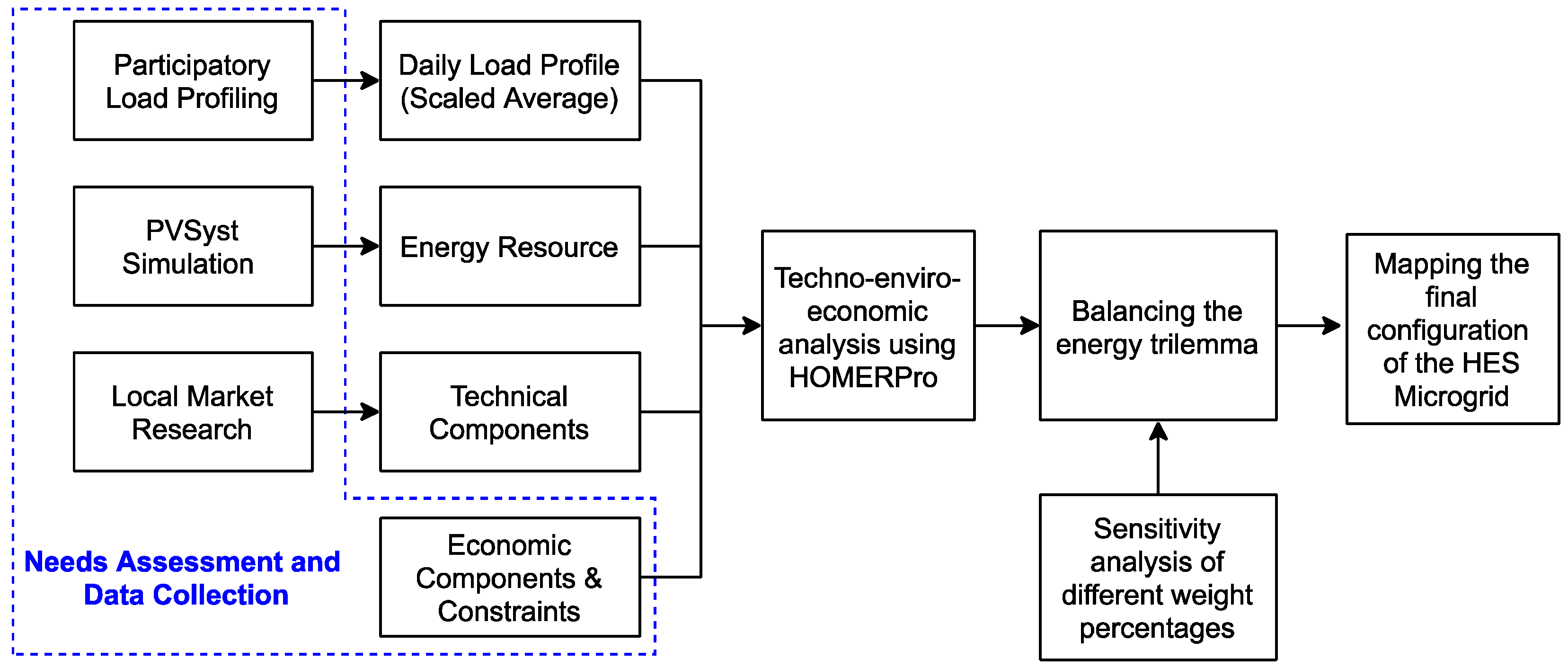
Conflicts of Interest

The authors declare no conflict of interest.

Abbreviations

The following abbreviations are used in the manuscripts:
ABCArtificial bee colony
ACSLAnnual capacity shortage limit
AEFAArtificial electric field algorithm
AFAffordability factor
AGAAdaptive genetic algorithm
BBattery
BDBiodiesel
BMBiomass
BOBonobo optimizer
CCCycle charging
COECost of electricity
CSACrow search algorithm
CSAAC-APCSA with an adaptive chaotic awareness probability
DGDiesel generator
DPSPDeficiency of power supply probability
DRSPDistributed rooftop solar PV
ETEnergy trilemma
FCFuel cell
FCCFixed capital cost
FPAFlower pollination algorithm
FPVFloating PV
FSCFeasible system configuration
GOAGrasshopper optimization algorithm
GPCGiza pyramids construction
GWOGrey wolf optimize
HASHarmony search algorithm
HESHybrid energy system
HHOHarris hawk’s optimization
HHSSAAHybrid harmony search-simulated annealing algorithm
HOMERHybrid Optimization Model for Multiple Energy Resources
IWOInvasive weed optimization
LCOELevelized cost of energy
LFLoad following
LPSPLoss of power supply probability
MOCSAMulti-objective crow search algorithm
NPCNet present cost
NSGA-IINon-dominated sorting genetic algorithm
O&MOperation and maintenance
OSCOptimum system configuration
PHSPump hydro storage
PSOParticle swarm optimization
PVPhotovoltaic
QOBOQuasi-oppositional BO
RERenewable energy
RFReliability factor
RPFRenewable penetration fraction
RSPRooftop solar PV
SAASimulated annealing algorithm
SOCState of charge
SSOSocial spider optimizer
TEETechno-environmental-economic
TCFThree core factors
TLBOTeaching–learning-based optimization
WTWind turbine

References

  1. The World Bank. More People Have Access to Electricity Than Ever Before, but World Is Falling Short of Sustainable Energy Goals, World Bank. 2019. Available online: https://www.worldbank.org/en/news/press-release/2019/05/22/tracking-sdg7-the-energy-progress-report-2019 (accessed on 2 October 2019).
  2. National Electrification Administration. NEA 2020 Annual Report. Manila, Philippines January 2021. Available online: https://www.nea.gov.ph/ao39/phocadownload/Annual_Reports//NEA%202020%20Annual%20Report.pdf (accessed on 22 October 2021).
  3. United Nations. Transforming Our World: The 2030 Agenda for Sustainable Development. 2016. Available online: https://sustainabledevelopment.un.org/content/documents/21252030%20Agenda%20for%20Sustainable%20Development%20web.pdf (accessed on 2 May 2021).
  4. World Energy Trilemma Index|2019; World Energy Council: London, UK, 2019; Available online: https://www.worldenergy.org/assets/downloads/WETrilemma_2019_Full_Report_v4_pages.pdf (accessed on 29 April 2020).
  5. Jacobson, A. Connective Power: Solar Electrification and Social Change in Kenya. World Dev. 2007, 35, 144–162. [Google Scholar] [CrossRef]
  6. Chowdhury, S.A.; Mourshed, M.; Kabir, S.R.; Islam, M.; Morshed, T.; Khan, M.R.; Patwary, M.N. Technical appraisal of solar home systems in Bangladesh: A field investigation. Renew. Energy 2011, 36, 772–778. [Google Scholar] [CrossRef] [Green Version]
  7. Kurata, M.; Matsui, N.; Ikemoto, Y.; Tsuboi, H. Do determinants of adopting solar home systems differ between households and micro-enterprises? Evidence from rural Bangladesh. Renew. Energy 2018, 129, 309–316. [Google Scholar] [CrossRef]
  8. Opiyo, N.N. A comparison of DC-versus AC-based minigrids for cost-effective electrification of rural developing communities. Energy Rep. 2019, 5, 398–408. [Google Scholar] [CrossRef]
  9. Bertheau, P.; Cader, C. Electricity sector planning for the Philippine islands: Considering centralized and decentralized supply options. Appl. Energy 2019, 251, 113393. [Google Scholar] [CrossRef]
  10. Brent, A.C.; Rogers, D.E. Renewable rural electrification: Sustainability assessment of mini-hybrid off-grid technological systems in the African context. Renew. Energy 2010, 35, 257–265. [Google Scholar] [CrossRef] [Green Version]
  11. Ulsrud, K.; Winther, T.; Palit, D.; Rohracher, H.; Sandgren, J. Energy for Sustainable Development the Solar Transitions research on solar mini-grids in India: Learning from local cases of innovative socio-technical systems. Energy Sustain. Dev. 2011, 15, 293–303. [Google Scholar] [CrossRef]
  12. López-González, A.; Domenech, B.; Ferrer-Martí, L. Sustainability and design assessment of rural hybrid microgrids in Venezuela. Energy 2018, 159, 229–242. [Google Scholar] [CrossRef]
  13. Boliko, C.M.; Ialnazov, D.S. An assessment of rural electrification projects in Kenya using a sustainability framework. Energy Policy 2019, 133, 110928. [Google Scholar] [CrossRef]
  14. Hong, G.W.; Abe, N. Sustainability assessment of renewable energy projects for off-grid rural electrification: The Pangan-an Island case in the Philippines. Renew. Sustain. Energy Rev. 2012, 16, 54–64. [Google Scholar] [CrossRef]
  15. Meschede, H.; Esparcia, E.J.; Holzapfel, P.; Bertheau, P.; Ang, R.C.; Blanco, A.C.; Ocon, J.D. On the transferability of smart energy systems on o ff -grid islands using cluster analysis—A case study for the Philippine archipelago. Appl. Energy 2019, 251, 113290. [Google Scholar] [CrossRef]
  16. Lim, L. Mararison Solar pv Hybrid Project. 2019. Available online: https://events.development.asia/materials/20190619/malalison-island-solar-hybrid-project (accessed on 9 July 2020).
  17. IRENA. Mini-Grid Deployment: A Study on the Philippines; International Renewable Energy Agency: Abu Dhabi, United Arab Emirates, 2017; Available online: https://www.irena.org/-/media/Files/IRENA/Agency/Publication/2017/Oct/IRENA_Philippines_Renewable_Mini-Grids_2017.pdf (accessed on 12 October 2019).
  18. Stigka, E.K.; Paravantis, J.A.; Mihalakakou, G.K. Social acceptance of renewable energy sources: A review of contingent valuation applications. Renew. Sustain. Energy Rev. 2014, 32, 100–106. [Google Scholar] [CrossRef]
  19. Roche, O.; Blanchard, R. Design of a solar energy centre for providing lighting and income-generating activities for off-grid rural communities in Kenya. Renew. Energy 2018, 118, 685–694. [Google Scholar] [CrossRef] [Green Version]
  20. Akinyele, D. Techno-economic design and performance analysis of nanogrid systems for households in energy-poor villages. Sustain. Cities Soc. 2017, 34, 335–357. [Google Scholar] [CrossRef]
  21. Burmester, D.; Rayudu, R.; Seah, W.; Akinyele, D. A review of nanogrid topologies and technologies. Renew. Sustain. Energy Rev. 2017, 67, 760–775. [Google Scholar] [CrossRef]
  22. Rabuya, I.; Libres, M.; Abundo, M.; Taboada, E. Moving Up the Electrification Ladder in Off-Grid Settlements with Rooftop Solar Microgrids. Energies 2021, 14, 3467. [Google Scholar] [CrossRef]
  23. Shezan, S.; Julai, S.; Kibria, M.; Ullah, K.; Saidur, R.; Chong, W.T.; Akikur, R. Performance analysis of an off-grid wind-PV (photovoltaic)-diesel-battery hybrid energy system feasible for remote areas. J. Clean. Prod. 2016, 125, 121–132. [Google Scholar] [CrossRef]
  24. Rahman, M.; Khan, M.-U.; Ullah, M.A.; Zhang, X.; Kumar, A. A hybrid renewable energy system for a North American off-grid community. Energy 2016, 97, 151–160. [Google Scholar] [CrossRef]
  25. Bukar, A.L.; Tan, C.W.; Lau, K.Y. Optimal sizing of an autonomous photovoltaic/wind/battery/diesel generator microgrid using grasshopper optimization algorithm. Sol. Energy 2019, 188, 685–696. [Google Scholar] [CrossRef]
  26. Elkadeem, M.; Wang, S.; Sharshir, S.; Atia, E.G. Feasibility analysis and techno-economic design of grid-isolated hybrid renewable energy system for electrification of agriculture and irrigation area: A case study in Dongola, Sudan. Energy Convers. Manag. 2019, 196, 1453–1478. [Google Scholar] [CrossRef]
  27. Kharrich, M.; Mohammed, O.H.; Kamel, S.; Selim, A.; Sultan, H.M.; Akherraz, M.; Jurado, F. Development and Implementation of a Novel Optimization Algorithm for Reliable and Economic Grid-Independent Hybrid Power System. Appl. Sci. 2020, 10, 6604. [Google Scholar] [CrossRef]
  28. Yoshida, Y.; Farzaneh, H. Optimal Design of a Stand-Alone Residential Hybrid Microgrid System for Enhancing Renewable Energy Deployment in Japan. Energies 2020, 13, 1737. [Google Scholar] [CrossRef] [Green Version]
  29. Fathy, A.; Kaaniche, K.; Alanazi, T.M. Recent Approach Based Social Spider Optimizer for Optimal Sizing of Hybrid PV/Wind/Battery/Diesel Integrated Microgrid in Aljouf Region. IEEE Access 2020, 8, 57630–57645. [Google Scholar] [CrossRef]
  30. Quitoras, M.R.; Campana, P.E.; Rowley, P.; Crawford, C. Remote community integrated energy system optimization including building enclosure improvements and quantitative energy trilemma metrics. Appl. Energy 2020, 267, 115017. [Google Scholar] [CrossRef]
  31. Kotb, K.M.; Elkadeem, M.; Elmorshedy, M.F.; Dán, A. Coordinated power management and optimized techno-enviro-economic design of an autonomous hybrid renewable microgrid: A case study in Egypt. Energy Convers. Manag. 2020, 221, 113185. [Google Scholar] [CrossRef]
  32. Chen, H.-C. Optimum capacity determination of stand-alone hybrid generation system considering cost and reliability. Appl. Energy 2013, 103, 155–164. [Google Scholar] [CrossRef]
  33. Ahmadi, S.; Abdi, S. Application of the Hybrid Big Bang–Big Crunch algorithm for optimal sizing of a stand-alone hybrid PV/wind/battery system. Sol. Energy 2016, 134, 366–374. [Google Scholar] [CrossRef]
  34. Javed, M.S.; Song, A.; Ma, T. Techno-economic assessment of a stand-alone hybrid solar-wind-battery system for a remote island using genetic algorithm. Energy 2019, 176, 704–717. [Google Scholar] [CrossRef]
  35. Khan, A.; Javaid, N. Jaya Learning-Based Optimization for Optimal Sizing of Stand-Alone Photovoltaic, Wind Turbine, and Battery Systems. Engineering 2020, 6, 812–826. [Google Scholar] [CrossRef]
  36. Rezzouk, H.; Mellit, A. Feasibility study and sensitivity analysis of a stand-alone photovoltaic–diesel–battery hybrid energy system in the north of Algeria. Renew. Sustain. Energy Rev. 2015, 43, 1134–1150. [Google Scholar] [CrossRef]
  37. Das, B.K.; Zaman, F. Performance analysis of a PV/Diesel hybrid system for a remote area in Bangladesh: Effects of dispatch strategies, batteries, and generator selection. Energy 2019, 169, 263–276. [Google Scholar] [CrossRef]
  38. Odou, O.D.T.; Bhandari, R.; Adamou, R. Hybrid off-grid renewable power system for sustainable rural electri fi cation in Benin. Renew. Energy 2020, 145, 1266–1279. [Google Scholar] [CrossRef]
  39. Jamshidi, M.; Askarzadeh, A. Techno-economic analysis and size optimization of an off-grid hybrid photovoltaic, fuel cell and diesel generator system. Sustain. Cities Soc. 2019, 44, 310–320. [Google Scholar] [CrossRef]
  40. Maleki, A.; Askarzadeh, A. Artificial bee swarm optimization for optimum sizing of a stand-alone PV/WT/FC hybrid system considering LPSP concept. Sol. Energy 2014, 107, 227–235. [Google Scholar] [CrossRef]
  41. Samy, M.; Barakat, S.; Ramadan, H. Techno-economic analysis for rustic electrification in Egypt using multi-source renewable energy based on PV/ wind/ FC. Int. J. Hydrog. Energy 2019, 45, 11471–11483. [Google Scholar] [CrossRef]
  42. Moghaddam, M.J.H.; Kalam, A.; Nowdeh, S.A.; Ahmadi, A.; Babanezhad, M.; Saha, S. Optimal sizing and energy management of stand-alone hybrid photovoltaic/wind system based on hydrogen storage considering LOEE and LOLE reliability indices using flower pollination algorithm. Renew. Energy 2018, 135, 1412–1434. [Google Scholar] [CrossRef]
  43. Samy, M.; Barakat, S.; Ramadan, H. A flower pollination optimization algorithm for an off-grid PV-Fuel cell hybrid renewable system. Int. J. Hydrog. Energy 2019, 44, 2141–2152. [Google Scholar] [CrossRef]
  44. Guangqian, D.; Bekhrad, K.; Azarikhah, P.; Maleki, A. A hybrid algorithm based optimization on modeling of grid independent biodiesel-based hybrid solar/wind systems. Renew. Energy 2018, 122, 551–560. [Google Scholar] [CrossRef]
  45. Makhdoomi, S.; Askarzadeh, A. Optimizing operation of a photovoltaic/diesel generator hybrid energy system with pumped hydro storage by a modified crow search algorithm. J. Energy Storage 2019, 27, 101040. [Google Scholar] [CrossRef]
  46. Kharrich, M.; Kamel, S.; Alghamdi, A.; Eid, A.; Mosaad, M.; Akherraz, M.; Abdel-Akher, M. Optimal Design of an Isolated Hybrid Microgrid for Enhanced Deployment of Renewable Energy Sources in Saudi Arabia. Sustainability 2021, 13, 4708. [Google Scholar] [CrossRef]
  47. Temiz, M.; Javani, N. Design and analysis of a combined floating photovoltaic system for electricity and hydrogen production. Int. J. Hydrog. Energy 2020, 45, 3457–3469. [Google Scholar] [CrossRef]
  48. Li, Z.; Boyle, F.; Reynolds, A. Domestic application of solar PV systems in Ireland: The reality of their economic viability. Energy 2011, 36, 5865–5876. [Google Scholar] [CrossRef]
  49. Li, C.; Ge, X.; Zheng, Y.; Xu, C.; Ren, Y.; Song, C.; Yang, C. Techno-economic feasibility study of autonomous hybrid wind/PV/battery power system for a household in Urumqi, China. Energy 2013, 55, 263–272. [Google Scholar] [CrossRef]
  50. UL. New Feature in HOMER Pro Energy Modeling Software Strengthens Client Presentations. 2020. Available online: https://www.ul.com/news/new-feature-homer-pro-energy-modeling-software-strengthens-client-presentations (accessed on 20 April 2021).
  51. GPS Coordinates of Olango Island Group, Philippines. Available online: https://latitude.to/articles-by-country/ph/philippines/41955/olango-island-group (accessed on 29 April 2020).
  52. A Resolution, No.02, Series of 2018.pdf, 2017th ed.; Energy Regulatory Commission (ERC): Pasig City, Philippines, 2018.
  53. Lozano, L.; Querikiol, E.M.; Abundo, M.L.S.; Bellotindos, L.M. Techno-economic analysis of a cost-effective power generation system for off-grid island communities: A case study of Gilutongan Island, Cordova, Cebu, Philippines. Renew. Energy 2019, 140, 905–911. [Google Scholar] [CrossRef]
  54. Jordan, D.C.; Kurtz, S.R. Photovoltaic Degradation Rates-an Analytical Review. Prog. Photovolt. Res. Appl. 2011, 21, 12–29. [Google Scholar] [CrossRef] [Green Version]
  55. Philippine Department of Energy. 2020. Available online: https://www.doe.gov.ph/retail-pump-prices-visayas?ckattempt=1 (accessed on 18 October 2020).
  56. Trading Economics. Philippines Inflation Rate 1958–2021 Data 2022–2023 Forecast Calendar. 2021. Available online: https://tradingeconomics.com/philippines/inflation-cpi (accessed on 7 July 2021).
  57. Malaysia Central Bank Key Rates 2020. Available online: https://countryeconomy.com/key-rates/malaysia (accessed on 7 July 2021).
  58. Bhatia, M.; Angelou, N. Beyond Connections: Energy Access Redefined; The International Bank for Reconstruction and Development/The World Bank Group: Washington, DC, USA, 2015; Available online: https://www.worldbank.org/content/dam/Worldbank/Topics/Energy%20and%20Extract/Beyond_Connections_Energy_Access_Redefined_Exec_ESMAP_2015.pdf (accessed on 7 March 2019).
Figure 1. A schematic overview of the methodology used in this study.
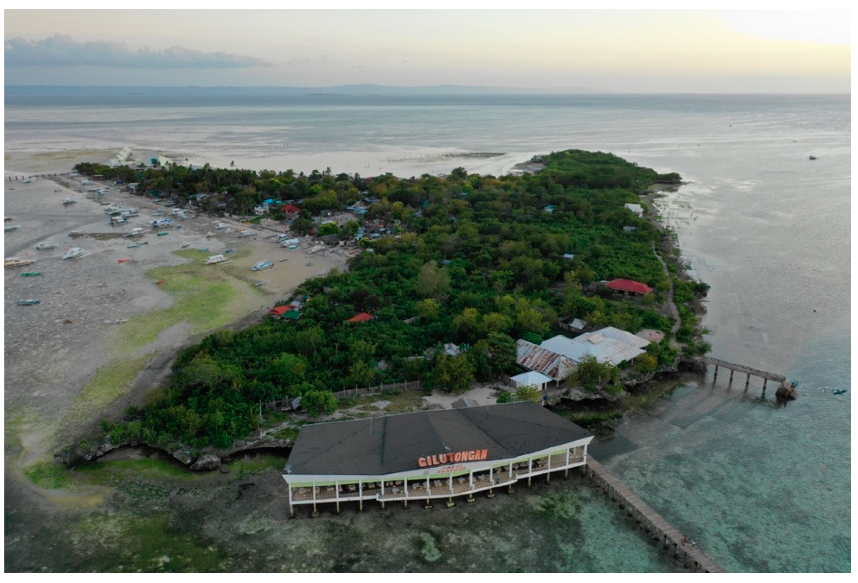
Energies 14 07358 g001
Figure 2. Gilutongan Island in Cordova, Cebu, Philippines.
Energies 14 07358 g002
Figure 3. Electrical distribution setup of Gilutongan Island.
Energies 14 07358 g003
Figure 4. Projected daily load profile for the 11 Households with 24-h electricity access.
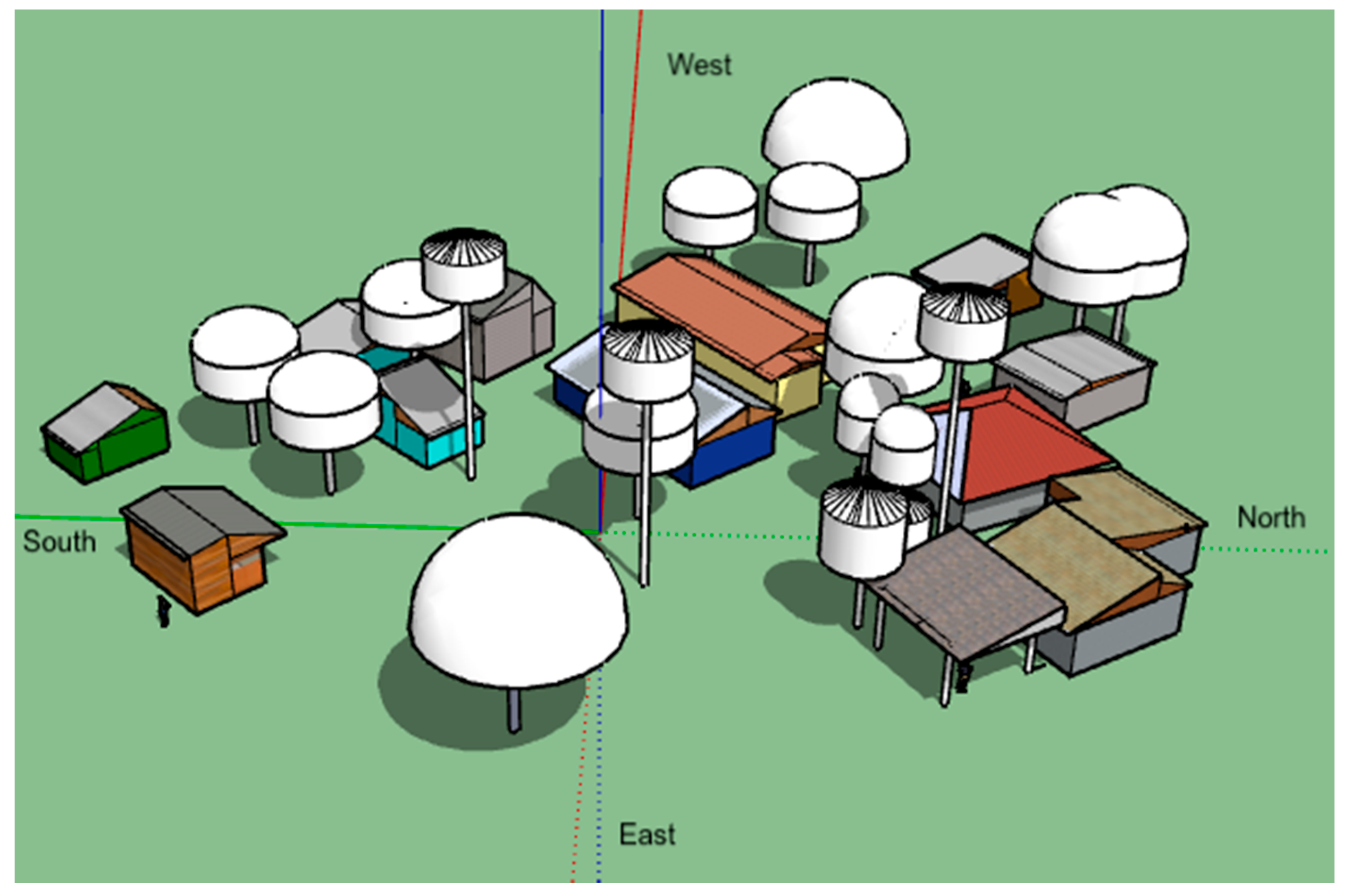
Energies 14 07358 g004
Figure 5. The 3D model of the actual 11 houses in the case study site.
Energies 14 07358 g005
Figure 6. Perspective of the rooftop PV field and surrounding shading scene.
Energies 14 07358 g006
Figure 7. Basic data of the JPS-330P-72 used in the PVSyst simulation.
Energies 14 07358 g007
Figure 8. Components of the HES microgrid.
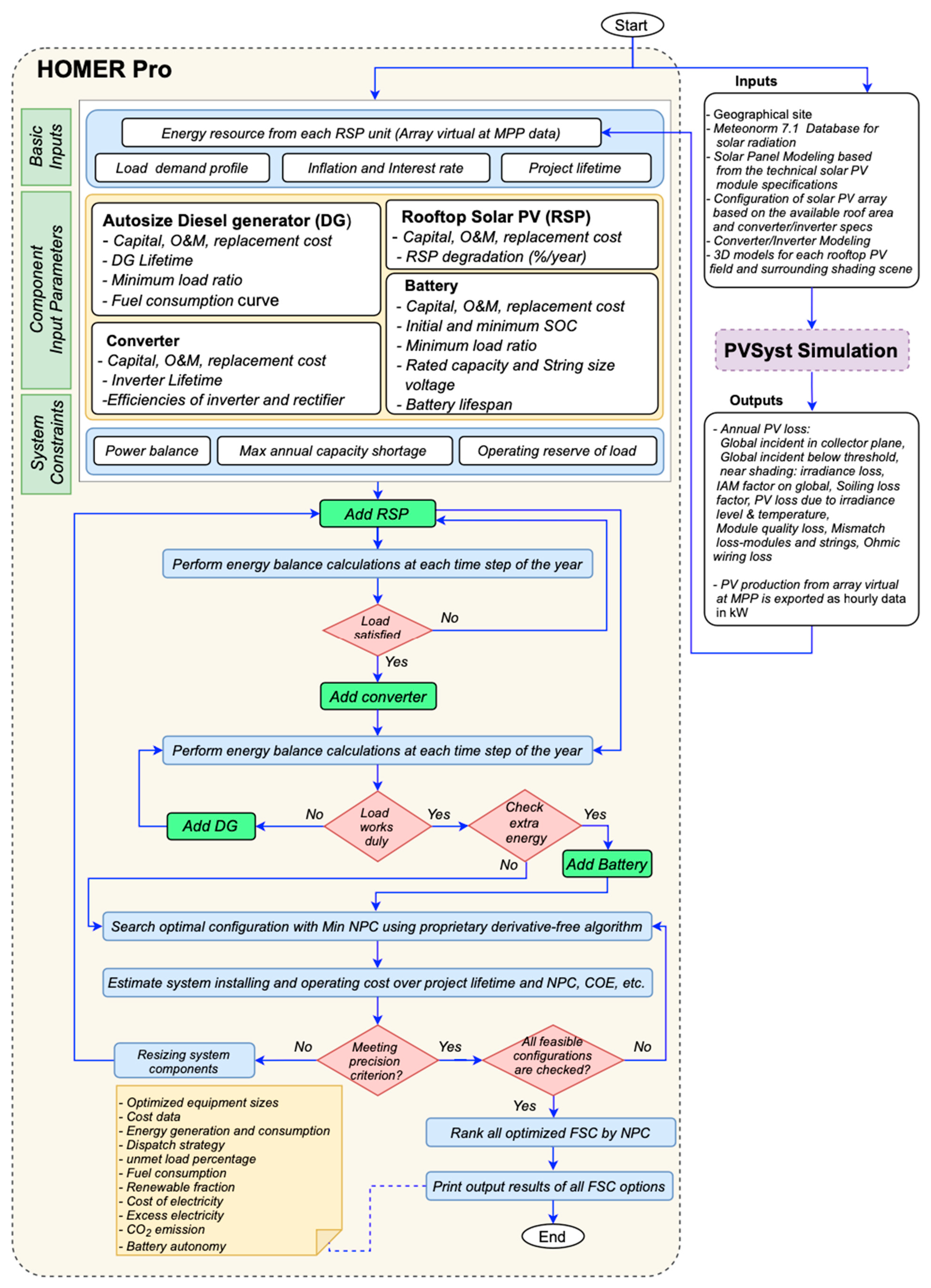
Energies 14 07358 g008
Figure 9. Procedure for the selection of all feasible system configurations (FSCs) using PVSyst and HOMER Pro.
Energies 14 07358 g009
Figure 10. Configuration of roof 2 (R2) as a PVSyst unit.
Energies 14 07358 g010
Figure 11. Graphical presentation of all FSCs that satisfy the load demand at 14.2 kWh/day.
Energies 14 07358 g011
Figure 12. Monthly electricity production of the OSC at 14.2 kWh/day.
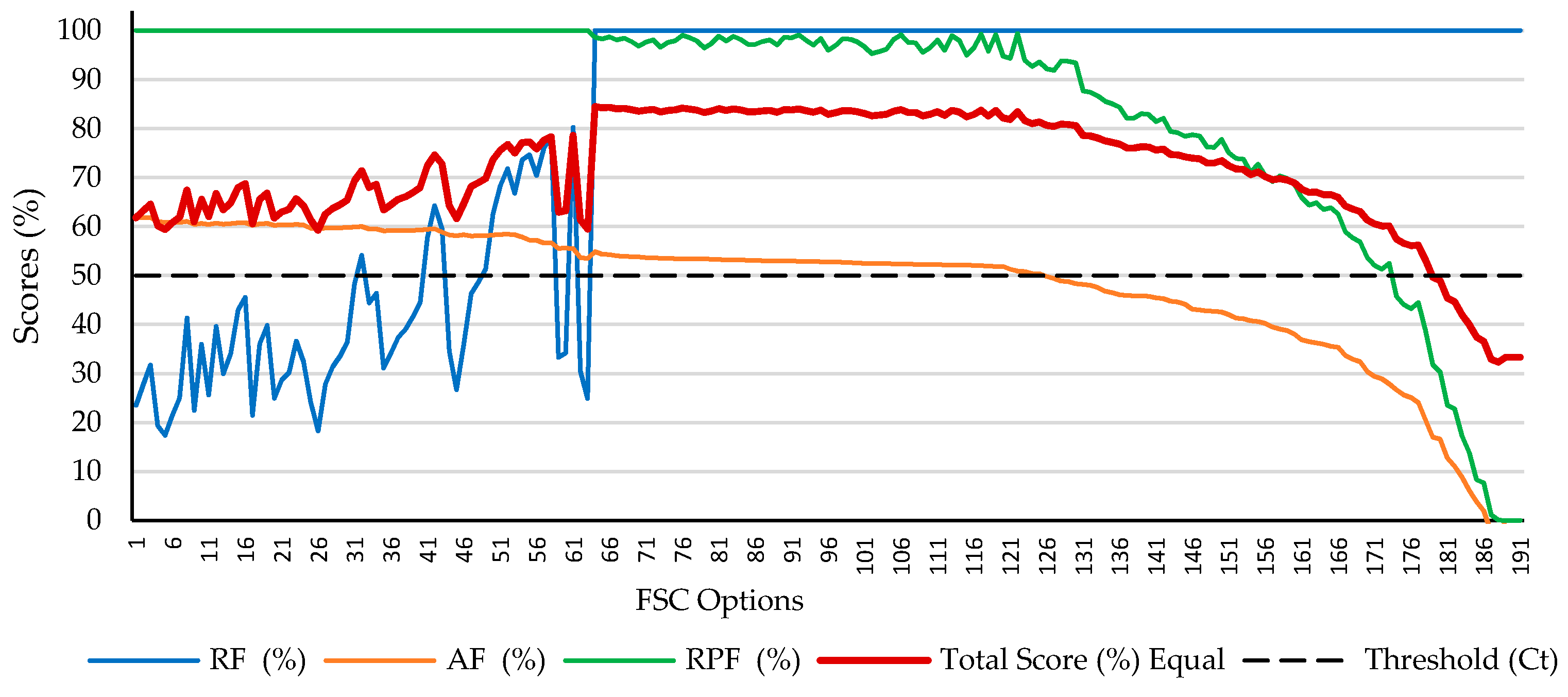
Energies 14 07358 g012
Figure 13. Graphical presentation of all FSCs that satisfy the load demand at 22 kWh/day.
Energies 14 07358 g013
Figure 14. HOMER’s time series simulation of the system during low solar PV production.
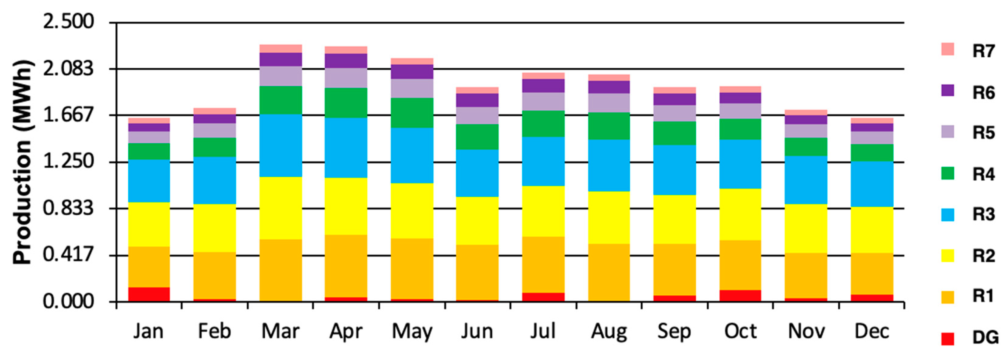
Energies 14 07358 g014
Figure 15. Monthly electricity production of the OSC at 22 kWh/day.
Energies 14 07358 g015
Figure 16. Graphical presentation of all FSCs that satisfy the load demand at 37.9 kWh/day.
Energies 14 07358 g016
Figure 17. Monthly electricity production of the OSC at 37.9 kWh/day.
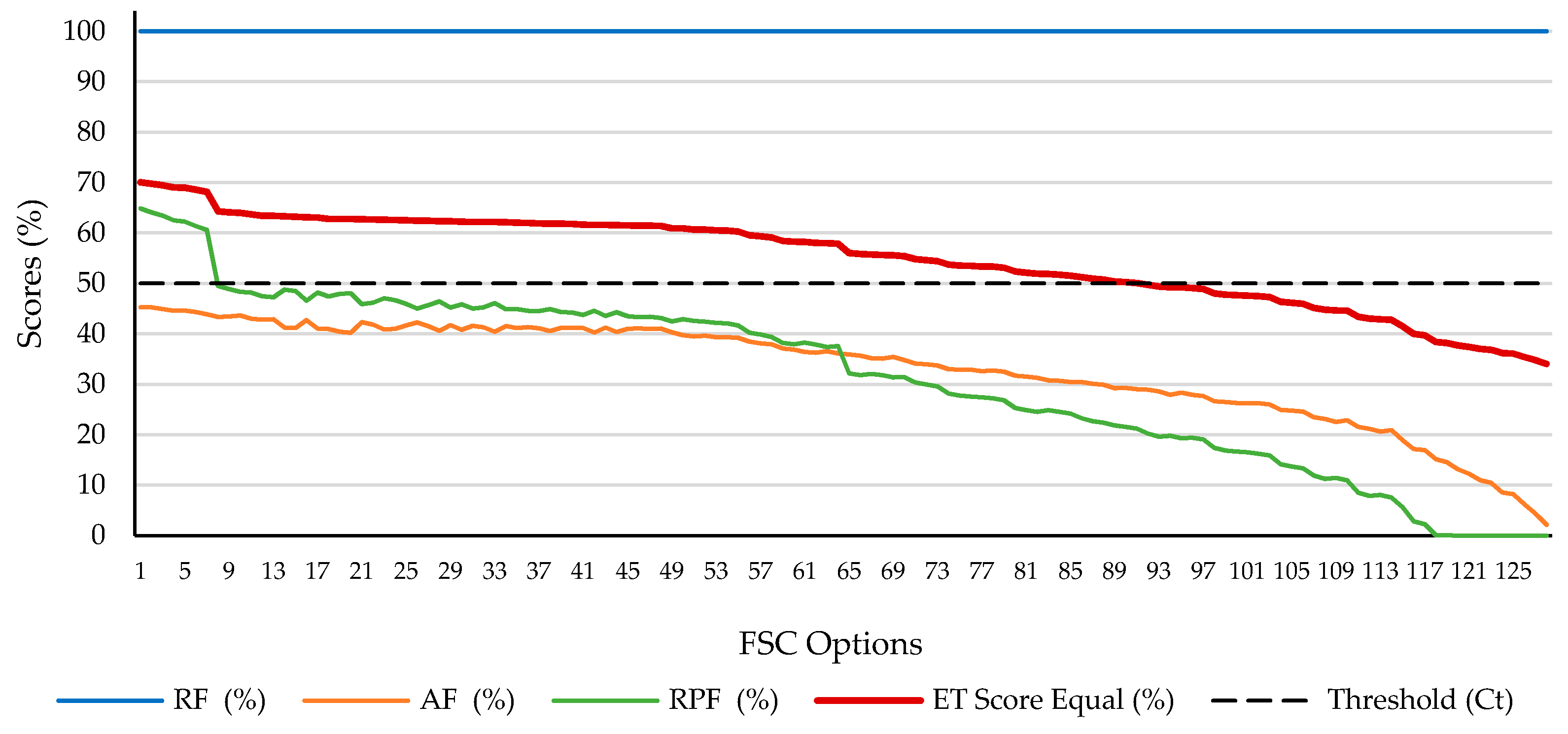
Energies 14 07358 g017
Figure 18. Graphical presentation of all FSCs that satisfy the load demand at 57.7 kWh/day.
Energies 14 07358 g018
Figure 19. Monthly electricity production of the OSC at 57.7 kWh/day.
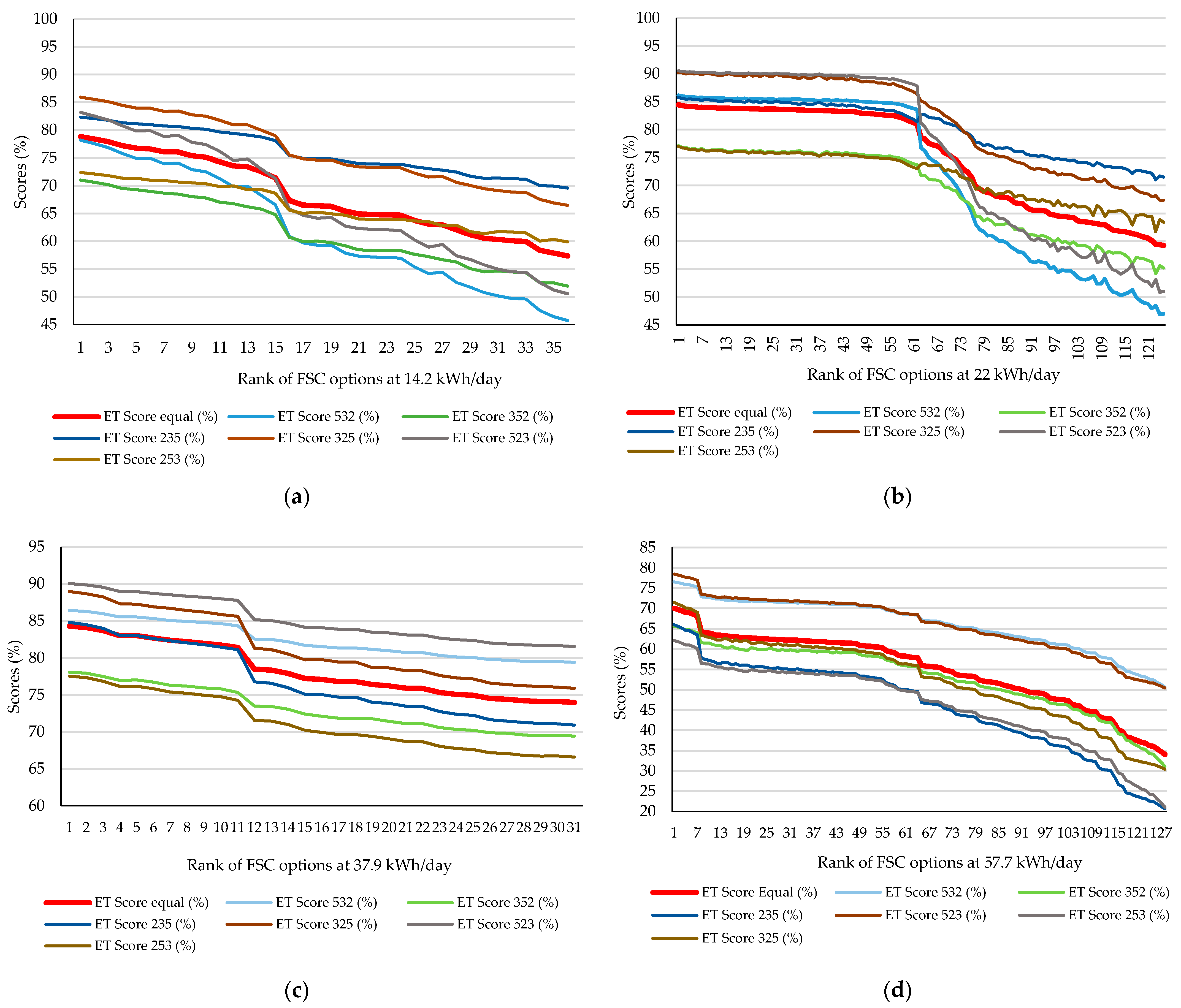
Energies 14 07358 g019
Figure 20. Effects of varying weight percentages on the OSC at (a) 14.2; (b) 22; (c) 37.9; and (d) 57.7 kWh/day.
Energies 14 07358 g020
Table 1. Summary of previous works with different objective functions and algorithms.
AuthorsYearHESLocationAlgorithm/ToolObjective Function
Shezan et al. [23]2016WT/PV/B/DGSelangor, Malaysia HOMERMinimized NPC and CO2 emission
Rahman et al. [24]2016WT/PV/B/DGSandy Lake First Nation, OntarioHOMERSatisfy the load demand with minimum NPC and COE
Bukar et al. [25]2019WT/PV/B/DGNigeriaGOASupply energy demand reliably based on DPSP and minimized COE
Elkadeem et al. [26]2019WT/PV/B/DGDongola, SudanHOMER ProLeast NPC and realistic environmental impact
Kharrich et al. [27]2020WT/PV/B/DGAswan, EgyptTraditional BO, QOBO, HHO, AEFA, IWOMinimized NPC and COE
Yoshida et al. [28]2020WT/PV/B/DGFukuoka, JapanPSOLeast-cost perspective
Fathy et al. [29]2020WT/PV/B/DGAlijouf region, Saudi ArabiaSSOMinimized COE and LPSP
Quitoras et al. [30]2020WT/PV/B/DGCanadaNSGA-IIMulti-domain perspective of balancing energy trilemma parameters (LPSP, excess electricity, LCC, LCOE, CO2 emission, RE penetration fraction)
Kotb et al. [31]2020PV/WT/DG/BEgyptHOMER and MATLAB/SIMULINKMinimized the life-cycle cost, energy cost and emission as well as capacity shortage fraction
Chen [32]2013WT/PV/BWuchiAGAPower system reliability and cost minimization
Ahmadi et al. [33]2016WT/PV/BQazvin, IranHBB-BCSatisfy the load demand and minimizing the total NPC
Javed et al. [34]2019WT/PV/BJiuduansha, islandGA and HOMERSatisfy the load requirements with lowest costs
Khan et al. [35]2020WT/PV/BRafsanjan, IranJaya, TLBO, JLBO, GASatisfy the consumer’s load at minimal total annual cost
Rezzouk et al. [36]2015PV/B/DGNorth of AlgeriaHOMERMaximum output power at a low cost (NPC & COE)
Das et al. [37]2019PV/B/DGBangladeshHOMERMinimized NPC and COE in relation to different dispatch strategy
Odou et al. [38]2020PV/B/DGAlibori, BeninHOMERMinimized NPC
Jamshidi et al. [39]2018PV/FC/DGKerman, south of IranMOCSATotal NPC and LPSP
Maleki et al. [40]2014PV/WT/FCRafsanjan, South of IranABSOMinimized total annual cost and maximum allowable LPSP
Samy et al. [41]2020PV/WT/FCEgyptFPAMinimized NPC with the LPSP of 2%
Hadidian et al. [42]2019PV/WT/FCNorthwest IranFPA, TLBO, PSOMinimized total NPC and reliability indices are considered
Samy et al. [43]2019PV/FCEgyptFPA, ABC, PSOMinimized total NPC and LPSP is considered
Guangqian et al. [44]2018PV/WT/BD/BKhorasan, IranHSA, SAA, HHSSAAMinimized life cycle cost (LCC)
Makhdoomi et al. [45]2020PV/DG/PHSAdrar, AlgeriaGA, PSO, CSA, CSAAC-APMinimum operation cost through fuel consumption
Kharrich et al. [46] 2021PV/BM and WT/PV/B/DGSaudi ArabiaGPC, AEFA, GWOMinimized NPC and considering LPSP and availability index
Temiz et al. [47]2020FPV/hydrogen FCSouthern TurkeyHOMER and PVSystUninterrupted electrical power supply and land conservation
Table 2. Estimated daily energy consumption for the 11 households.
HouseElectrical LoadPower Rating (W)QtyEstimated Daily Load Consumption (kWh/day)
EL 1STL 2MTL 3LTL 4
1Light Bulb1650.4160.4160.4160.416
Light Bulb910.0990.0990.0990.099
Television15010.750.750.750.75
Audio system15010.150.150.150.15
Electric fan5020.400.400.400.4
Fridge (MT plan)1651--3.963.96
2Light Bulb1130.1870.1870.1870.187
Electric fan5010.50.50.50.5
Television15010.60.60.60.6
Television5010.20.20.20.2
Rice cooker80012.42.42.42.4
Fridge (ST plan)1651-3.963.963.96
3Light Bulb510.080.080.080.08
Television15010.60.60.60.6
Fridge (MT plan)1651--3.963.96
4Light Bulb510.020.020.020.02
Light Bulb1810.090.090.090.09
Light Bulb710.0350.0350.0350.035
Light Bulb1310.0520.0520.0520.052
Television5010.250.250.250.25
Fridge (MT plan)1651--3.963.96
5Light Bulb910.1170.1170.1170.117
Light Bulb2210.1320.1320.1320.132
Audio system80011.601.601.601.60
Television4010.400.400.400.40
Electric Fan5010.300.300.300.30
Fridge (MT plan)1651--3.963.96
6Light Bulb2510.250.250.250.25
Light Bulb1110.0330.0330.0330.033
Fridge (LT plan)1651---3.96
7Light Bulb910.1530.1530.1530.153
Television4510.270.270.270.27
Fridge (LT plan)1651---3.96
8Light Bulb2010.1400.1400.1400.140
Television5010.250.250.250.25
Ceiling fan3010.690.690.690.69
Electric fan5011.001.001.001.00
Fridge (ST plan)1651-3.963.963.96
9Light Bulb1810.0720.0720.0720.072
Light Bulb510.0450.0450.0450.045
Fridge (LT plan)1651---3.96
10Light Bulb2320.5060.5060.5060.506
Light Bulb910.0990.0990.0990.099
Television15010.900.900.900.90
Fridge (LT plan)1651---3.96
11Light Bulb910.1530.1530.1530.153
Light Bulb810.040.040.040.04
Fridge (LT plan)1651---3.96
Total energy demand per day (kWh/day)14.22237.957.7
1 Existing load (EL), 2 Short-term load (STL), 3 Medium-term load (MTL), 4 Long-term load (LTL).
Table 3. The details of Converter model parameters.
Converter (Axpert MKS 5K-48)
Sizes considered (kW)0, 5, 10
Control inverter efficiency93%
Parallel with AC GeneratorYes
Rectifier relative capacity100%
Rectifier relative capacity98%
Table 4. Auto-size genset default properties.
Fuel curveEmissionsFuel Properties
Intercepts (0.369 L/h)Carbon Monoxide (CO)(16.5 g/L fuel)Lower Heating Value(43.2 MJ/kg)
Slope (0.236 L/h/kW)Unburned Hydrocarbons (UHC)(0.72 g/L fuel)Density(820 kg/m3)
Particulates(0.1 g/L fuel)Carbon Content(88%)
Fuel Sulfur to Particulate
Matter (PM)
(2.2%)Sulfur Content(0.4%)
Nitrogen Oxides (NOx)(15.5 g/L fuel)
Table 5. Energy Trilemma (ET) index used in the ET scoring.
Three Core Factors (TCF) Parameters Used
Reliability (RF)
-
Unmet load fraction
Affordability (AF)
-
LCOE of the FSC
-
COE threshold limit of USD 0.336 per kWh
Environmental Sustainability (ES)
-
Renewable penetration fraction (RPF)
Table 6. Sensitivity parameters for different weight percentages in the ET scoring.
Total Score (%)RF * (a)AF * (b)ES * (c)
ET score-111RF * (100%)AF * (100%)ES * (100%)
ET score-532RF * (50%)AF * (30%)ES * (20%)
ET score-352RF * (30%)AF * (50%)ES * (20%)
ET score-235RF * (20%)AF * (30%)ES * (50%)
ET score-325RF * (30%)AF * (20%)ES * (50%)
ET score-523RF * (50%)AF * (20%)ES * (30%)
ET score-253RF * (20%)AF * (50%)ES * (30%)
Table 7. Summary of the annual PV loss diagram and its unique characteristics from the 7-rooftop solar PV.
Rooftop Solar PV (RSP)R1R2R3R4R5R6R7
Horizontal global irradiance (kWh/m2)1801180118011801180118011801
Global incident in collector plane (%)−3.0+1.0+0.9−7.7−4.9−13.6−4.9
Global incident below threshold (%)−0.1−0.1−0.1−0.1−0.1−0.1−0.1
Near shading: irradiance loss (%)−3.2−8.7−11−9.5−38.2−6.5−50.7
IAM factor on global (%)−3.3−2.8−2.8−3−3.3−3.5−3.4
Soiling loss factor (%)−3−3−3−3−3−3−3
Effective irradiance on collectors (kWh)36,45536,45536,45516,96816,96881668166
PV conversion: Eff. at STC (%)17171717171717
Array nominal energy at STC Eff.(kWh)628062006030280119671348783
PV loss due to irradiance level (%)−0.7−0.8−0.8−1−1.8−1−2.6
PV loss due to temperature (%)−8.0−8.0−7.9−7.4−6.2−7.5−5.7
Module quality loss (%)+0.4+0.4+0.40.4−0.40.4−0.4
Mismatch loss, modules and strings (%)−1.1−1.1−1.1−1.1−1.1−1.1−1.1
Ohmic wiring loss (%)−0.9−0.9−0.9−0.8−0.6−0.8−0.6
Array virtual at MPP (kWh)564554905423252917871216710
Roof orientation (tilt°/azimuth°)11/14710/−3314/−3327/−11827/6230/15234/−29
Roof plane area (m2)232323121266
Capacity (kW)3.963.963.961.981.980.990.99
O&M cost (USD/year)39.639.639.61.981.980.990.99
Cost for retrofit (USD)600600600600600600600
Solar PV capital cost170417041704852852426426
Total Initial capital cost2304230423041452145210261026
Table 8. Optimization results of the top 10 FSCs and the conventional DG alone based on the ET scoring at 14.2 and 22 kWh/day.
DL 1FSC 2ArchitectureCostSystem3 Core Factors of ETETS 21 (%)Rank
Roof No.DG 3LA 4CV 5DS 6NPC 9COE 10OP 11IC 12TF 13EX 14UL 15CO 16AT 17RF 18AF 19ES 20
1234567(%)(%)(%)
14.24111 1 -125CC 831,9620.33479017,300031.310.69024.986.2650.2510078.841
421 11 -125CC 831,9620.33579017,300031.030.75024.984.9950.2210078.402
40 111 -125CC 831,9610.33579017,300030.370.82024.983.5650.1910077.923
4311 1 -125CC 831,9820.33579117,300028.110.92024.981.5250.1010077.214
3111 1 -125CC 831,3640.32978016,874025.631.04024.979.2551.0110076.755
441 1 1 -125CC 831,9880.33679117,300027.841.09024.979.8150.0510076.626
321 1 1 -125CC 831,3690.33078116,874025.371.13024.977.3050.9610076.097
39 11 1 -125CC 831,9500.33678917,300027.191.09024.978.1350.0710076.078
28 11 1 -125CC 831,3360.33077916,874024.721.24024.975.2250.9610075.399
2911 1-125CC 831,3420.33077916,874023.491.28024.974.4450.9310075.1210
232 12--CC 8854,1234.75025,412940012,07780.3031,613-1000033.33232
2264111 12245LF 745,2360.30380630,27252.128.310136.432.110054.8698.5984.481
661111 12205LF 745,8280.30782630,48447.539.350124.326.810054.2798.7184.332
65111 1 12205LF 745,7720.30784630,05862.633.710163.826.810054.3298.3084.213
761111 1 12205LF 746,6680.31381631,51036.744.60096.126.810053.4399.0084.144
68111 1 12205LF 746,1860.31084630,48456.836.160148.726.810053.9198.4684.125
811111 112205LF 746,8360.31482531,51041.642.410108.826.810053.2698.8784.046
67111 112205LF 746,0790.30986330,05871.631.570187.526.810054.0298.0684.027
9211111 12205LF 747,1840.31682131,93634.147.08089.226.810052.9199.0884.008
77111 11 12205LF 746,9550.31583231,51044.141.390115.526.810053.1498.8083.989
83111 1112205LF 746,6940.31384131,08454.436.750142.326.810053.4098.5383.9810
192 12 CC 8854,4143.07024,367940012,08469.5031,632-1000033.33192
1 Daily load consumption (kWh/day), 2 Feasible system configuration option from HOMER Pro, 3 Diesel generator size in kW, 4 Lead acid battery quantities, 5 Converter size in kW, 6 Dispatch strategy, 7 Load following, 8 Cycle charging, 9 Net Present Cost in USD, 10 Cost of electricity in USD/kWh, 11 Operating cost per year in USD/year, 12 Initial capital cost in USD, 13 Total fuel consumption per year (L/year), 14 Excess of electricity (%), 15 Unmet load (%), 16 Carbon emission in kg/year, 17 Battery autonomy in hours, 18 Reliability factor, 19 Affordability factor, 20 Environmental sustainability factor, 21 Energy trilemma score at equal percentage.
Table 9. Summary of energy production of the OSC at 14.2 kWh/day.
ProductionkWh/yearContribution
R1564541.3%
R2549040.2%
R3252918.5%
Total13,664100%
Table 10. Summary of energy production of the OSC at 22 kWh/day.
ProductionkWh/yearContribution
R1564529.4%
R2549028.6%
R3542328.3%
R4252913.2%
DG810.423%
Total19,168100%
Table 11. Optimization results of the top 10 FSCs and the conventional DG alone based on the ET scoring at 37.9 and 57.7 kWh/day.
DL 1FSC 2ArchitectureCostSystem3 Core Factors of ETETS 21 (%)Rank
Roof No.DG 3LA 4CV 5DS 6NPC 9COE 10OP 11IC 12TF 13EX 14UL 15CO 16AT 17RF 18AF 19ES 20
1234567(%)(%)(%)
37.911111111123210LF 772,0620.281180038,628341.925.910894.924.910058.2694.6284.291
2111111 123210LF 772,0760.281185637,602379.823.230994.124.910058.2594.0284.092
311111 1123210LF 773,2410.285191937,602416.121.4101089.224.910057.5793.4583.673
41111 1112325LF 773,8370.287202436,256525.620.1601375.924.910057.2391.7382.984
511111 12325LF 773,5690.286204235,656535.819.6801402.524.910057.3891.5782.985
61111 1 12325LF 774,1520.289209635,230572.817.6301499.424.910057.0590.9882.686
7111 11112325LF 775,6190.294212036,256578.217.5201513.524.910056.2090.9082.367
81111 112325LF 775,5420.294217135,230616.115.9301612.824.910056.2490.3082.188
9111 11 12325LF 776,1840.297220535,230633.015.0801657.024.910055.8790.0381.979
101111 12325LF 776,2260.297226334,204675.013.5601767.024.910055.8489.3781.7410
129 12 CC 8862,1251.824,589940012,27249032,124-1000033.33129
57.71111111112325CC 8143,9100.368571937,7082608.115.560682716.310045.2464.8770.041
2111111 12325CC 8143,8970.368577436,6822657.313.790695616.310045.2564.0669.772
311111 112325CC 8144,8270.370582436,6822695.712.580705616.310044.8963.4469.443
41111 1112325CC 8145,6990.373589436,2562754.111.360720916.310044.5662.5169.024
511111 12325CC 8145,4890.372591535,6562769.711.090725016.310044.6462.2668.975
61111 1 12325CC 8146,3430.374598435,2302826.19.870739816.310044.3261.3768.566
71111 112325CC 8147,4950.377604635,2302873.78.820752216.310043.8860.5868.157
8111 111122410CC 8148,8510.381614734,6963117.315.430816012.210043.3649.5164.298
9111 11 122410CC 8148,6230.380619033,6703155.613.720826012.210043.4548.8964.119
101111 122410CC 8148,1480.379622032,6443189.812.700835012.210043.6348.3463.9910
129 12 CC 8890,6461.2225,412940012,96829.9033,946-1000033.33129
1 Daily load consumption (kWh/day), 2 Feasible system configuration option from HOMER Pro, 3 Diesel generator size in kW, 4 Lead acid battery quantities, 5 Converter size in kW, 6 Dispatch strategy, 7 Load following, 8 Cycle charging, 9 Net Present Cost in USD, 10 Cost of electricity in USD/kWh, 11 Operating cost per year in USD/year, 12 Initial capital cost in USD, 13 Total fuel consumption per year (L/year), 14 Excess of electricity (%), 15 Unmet load (%), 16 Carbon emission in kg/year, 17 Battery autonomy in hours, 18 Reliability factor, 19 Affordability factor, 20 Environmental sustainability factor, 21 Energy trilemma score at equal percentage.
Table 12. Comparison of the final OSC at four case scenarios.
ParametersUnitOptimization Results
Case 1:
14.2 kWh/day
Case 2:
22 kWh/day
Case 3:
37.9 kWh/day
Case 4: 1
57.7 kWh/day
RSP-R1/R2/R4R1/R2/R3//R4R1/R2/R3//R4/R5/R6/R7R1/R2/R3//R4/R5/R6/R7
RSP energy productionkWh/year13,66419,08722,80022,800
200 AH LABsQty12203232
Battery bank usable capacitykWh14.724.539.339.3
ConverterkW55105
DGkW-121212
DG fuel consumptionL/year-47.5341.92608.1
Dispatch strategy-CCLFLFCC
Unmet load%0.65000
Excess electricity%31.4539.3525.9115.56
CO2 emissionsKg/year-124.3894.96827
Potential CO2 reduction%10099.6197.2179.89
COEUSD/kWh0.3340.3070.2810.368
NPCUSD31,96245,82872,062143,910
RF%86.26100100100
AF%50.2554.2758.2645.24
ES %10098.7194.6264.87
ET score%78.8484.3384.2970.04
1 The OSC in this case scenario is not economically viable for the 11 households.
Publisher’s Note: MDPI stays neutral with regard to jurisdictional claims in published maps and institutional affiliations.

