
On the Power Lines—Electromagnetic Shielding Using Magnetic Steel Laminates
by
 , , , and
Tatiana Damatopoulou
* ,
,
Spyros Angelopoulos
,
Christos Christodoulou
,
Ioannis Gonos
 ,
,
Evangelos Hristoforou
 and
and
Antonios Kladas

School of Electrical & Computer Engineering, National Technical University of Athens, Zografou Campus, 15780 Athens, Greece
*
Author to whom correspondence should be addressed.
Energies 2021, 14(21), 7215; https://doi.org/10.3390/en14217215
Submission received: 25 September 2021
/
Revised: 25 October 2021
/
Accepted: 26 October 2021
/
Published: 2 November 2021
(This article belongs to the Special Issue Advanced Electrical Measurements Technologies)
Abstract
:Protection against the electromagnetic fields around high-voltage transmission lines is an issue of great importance, especially in the case of buildings near power lines. Indeed, the developed fields can be harmful for the habitants and electrical/electronic devices, so the implementation of appropriate measures to address the above electromagnetic interference issue is necessary in order to ensure the safety of both human beings and equipment. Several practices have been proposed to reduce the electric and the magnetic fields around overhead and underground transmission lines (minimum distance, shielded cables, anechoic chamber etc.). In this context, the scope of the current paper is the use of highly permeable magnetic sheets for shielding purposes, along with the development of an appropriate procedure, based on finite element analysis (FEA) for the efficient design of passive shielding. The simulation results are compared with laboratory measurements in order to confirm the adequacy of the proposed methodology. The good agreement between the FEA outcomes and the experimental results confirms that the developed FEA tool can be trustfully used for the design of the shielding means in the case of overhead or underground power lines.
1. Introduction
There are several cases for which electromagnetic shielding is needed in domestic and industrial applications [1,2,3]. The most important issue is related to the effect of electromagnetic fields on humans and animals [4,5,6]. Several medical studies have been reported, related to people living close by overhead or underground power lines, with contradictory results [7,8,9,10].
Apart from this serious problem, electromagnetic interference on electronic systems is a well-observed and explainable issue [11]. The high amplitude 50 Hz electromagnetic field and the corresponding harmonics interfere with power supplies and low-frequency electronic circuitry, affecting their operation [12]. An interesting publication discussing these issues and the related standards is given in [13].
One of the most apparent problems is related to existing illegal constructions, such as houses being closer than 25 m to power transmission lines. Apart from the rising legal issues, the effect of the electromagnetic field on habitants and the related instrumentation are important engineering problems that must be sorted out properly.
International and national standardization and engineering institutions have studied the maximum acceptable amplitudes of interfering electric and magnetic fields, and they have concluded via international and national standards on proposals/suggestions for the highest allowable amplitudes of these fields. In several cases, these proposals/suggestions have been adopted as national laws. Accordingly, in the European Union, the maximum allowable amplitudes of electric fields are in the order of 5 kV/m and 10 kV/m concerning living and working places, respectively, while the maximum allowable amplitudes of magnetic fields for living and working places are 100 μT and 200 μT, respectively. Several international organizations such as the ICNIRP and IEEE proposed exposure limits linked to acute effects on the central nervous system (CNS). Based on ICNIR (1998) and on IEEE (2002), the guidelines for the general public and for personnel are presented in Table 1. The differences between the ICNIR and IEEE guidelines can be explained by the use of different adverse reaction thresholds, different safety measures and different transition frequencies. A working group on non-ionizing radiation was founded in 1974 by the International Radiation Protection Association, which analyzed protection-related problems against different types of non-ionizing radiation (NIR). A few years later in Paris, this working group was renamed the International Non-Ionizing Radiation Committee (INIRC). A cooperation between INIRC and the World Health Organization (WHO) followed, and various health criteria documents on NIR were established. Exposure limits were based on those health criteria. In 1992, INIRC became ICNIRP. The committee’s purpose is to analyze the hazards that may be linked to the various types of NIR, to publish international guidelines on NIR exposure limits and to review all perspectives of NIR protection.
To date, several practices and technologies have been developed to face this electromagnetic interference problem. The most usual and rather obvious solution is the obligation of a minimum distance between power lines and living and working places. This solution has been law for several countries around the world.
Another solution, particularly for underground power lines, is the fabrication and use of shielded cables, being an expensive but well-operating solution. In most cases, these cables use copper shielding for eddy current-based shielding and magnetic ribbons/films/wires for magnetic field absorption, accompanied by anti-corrosive polymeric substrates. Eddy currents oppose the transmitted magnetic field, while magnetic materials absorb this magnetic field. According to our understanding, magnetic field absorption is far better, concerning the 50 Hz field shielding, for several reasons, provided that the magnetic material is highly permeable and correspondingly non-expensive.
Another solution, especially useful for industrial and research environments, is anechoic chambers, equipped with metal films (usually aluminum) for eddy current generation and field cancellation for higher frequencies, as well as with magnetic metal films (usually permalloy) for field trapping/absorption. These chambers are a relatively expensive solution and offer passive field shielding, while in some cases, they implement active field cancelation by applying an opposing magnetic field to the field transmitted inside the volume of the anechoic chamber. For this reason, the employment of ultra-low carbon steels or electric steels offers a sustainable solution due to the relatively low cost and high levels of magnetic permeability (permeability for short).
The motivation of this paper is the use of highly permeable magnetic sheets for magnetic shielding purposes, namely low-cost electric steels or highly permeable ultra-low carbon magnetic sheets as shielding means, as well as the establishment of an algorithm allowing for the correct design of passive shielding based on finite element analysis (FEA), together with a corresponding experimental proof of principle. The comparison and the resulting good agreement between the specific FEA tools and the experimental results allow for the trustful use of the specific FEA tool selected after the proper determination of the uncertainties involved in the monitored magnetic field. Therefore, this FEA tool may well be the design tool for shielding means for the case of air or ground power lines.
In the following chapter (Section 2), the shielding materials are illustrated, while in Section 3, the finite element analysis (FEA) based on the soft magnetic properties of the shielding material is presented. Correspondingly, in Section 4, the experimental results and the comparison between the FEA results and the experiments are provided. Finally, in the Discussion, the developed algorithm is proposed, together with some important applications of the method related to house shielding and other applications.
2. The Shielding Material
The shielding material should be a highly soft magnetic material in order to maximize the trapping effect of the magnetic lines and, therefore, optimize the shielding process [14]. The most important highly soft magnetic materials are permalloys [15], amorphous and nano-crystalline ribbons and wires [16] and electric steels [14].
Permalloys, consisting of the NixFe1−x composition, offer excellent soft magnetic properties with maximum permeability levels in the order of 106. However, their high cost, in the order of 100 EUR/kg, makes them rather non-usable at a large scale.
Amorphous and nano-crystalline ribbons and wires have similar properties to permalloys with maximum permeability in the order of 105–106. However, nano-crystalline ribbons and wires suffer from a high level of fragility, thus prohibiting them from being manufactured for shielding applications. In addition, amorphous ribbons and wires cannot be welded and manufactured, becoming crystalline and, therefore, losing their excellent soft magnetic properties.
However, single-phase ultra-low carbon steels and electric steels offer maximum permeability from 104 to 105, maintain their properties after some welding processes and maintain a relatively low price in the order of 1000 EUR per ton. Finally, the repeatability of the magnetic, electric and mechanical properties of electric steels permitted their exclusive use as the proper shielding material for our studies.
The composition of electric steels is mainly Fe with a small percentage of Si (1.5–3%), as well as other elements, such as C and S (less than 10 ppm each). They are one of the most well-studied and explored families of soft magnetic materials. The method of their production is mainly hot extrusion, with subsequent heat treatment and magnetic annealing, thus controlling their microstructure and, therefore, their magnetization loop and magnetic losses. Different metallurgical processes may result in grain-oriented (GO) and non-oriented (NO) steel sheets [17], with the main difference being the presence of single-domain grains or multiple-domain grains. This way, their applications may vary from transformers to electric motors, chocks etc.
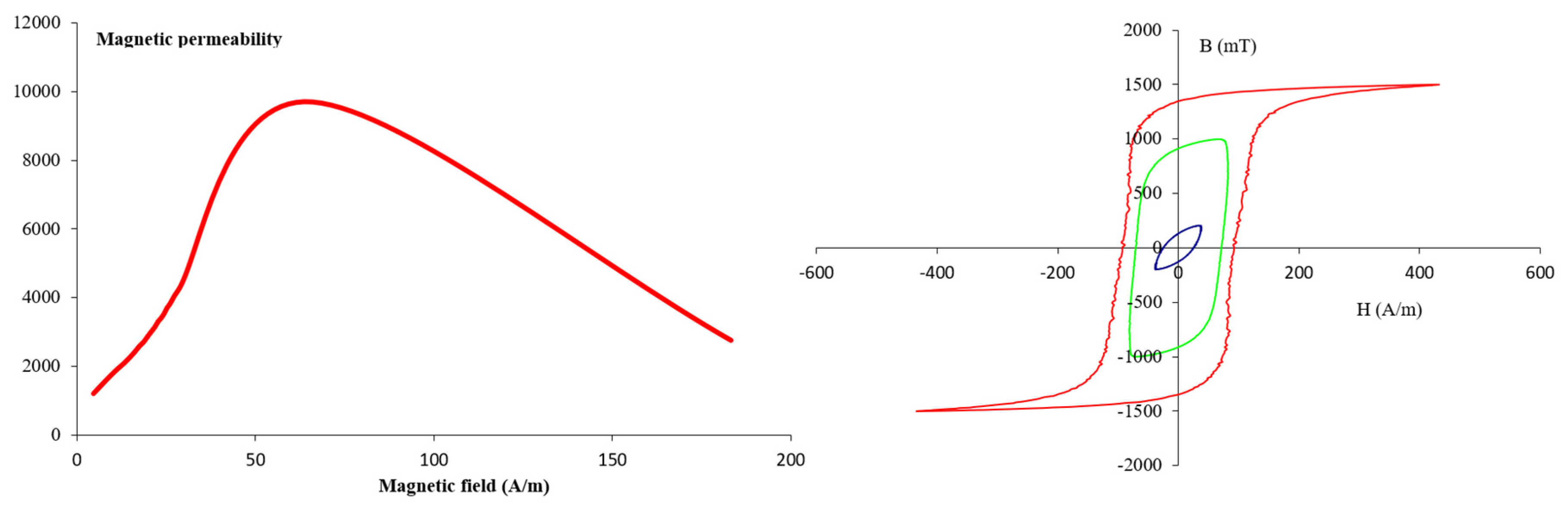
For the purpose of our applications, ultra-low carbon steel, or electric steel, is required in order to achieve high levels of magnetization. The proper development of these steels should result in a low level of residual stresses, or a low dislocation density, which would give the possibility of high permeability values. Thus, the need for non-destructive methods able to perform the determination of the magnetic permeability along the length and the width of the ultra-low carbon steel or the electric steel became a necessity [18]. Therefore, the single-sheet testing (SST) method [19] and the electromagnetic yoke (EMY) method [20] were adopted in order to achieve such two-dimensional permeability characterization. These results were achieved by monitoring the magnetization loop and, therefore, the magnetic permeability. The typical response of the magnetization loop and the corresponding magnetic permeability are illustrated in Figure 1.
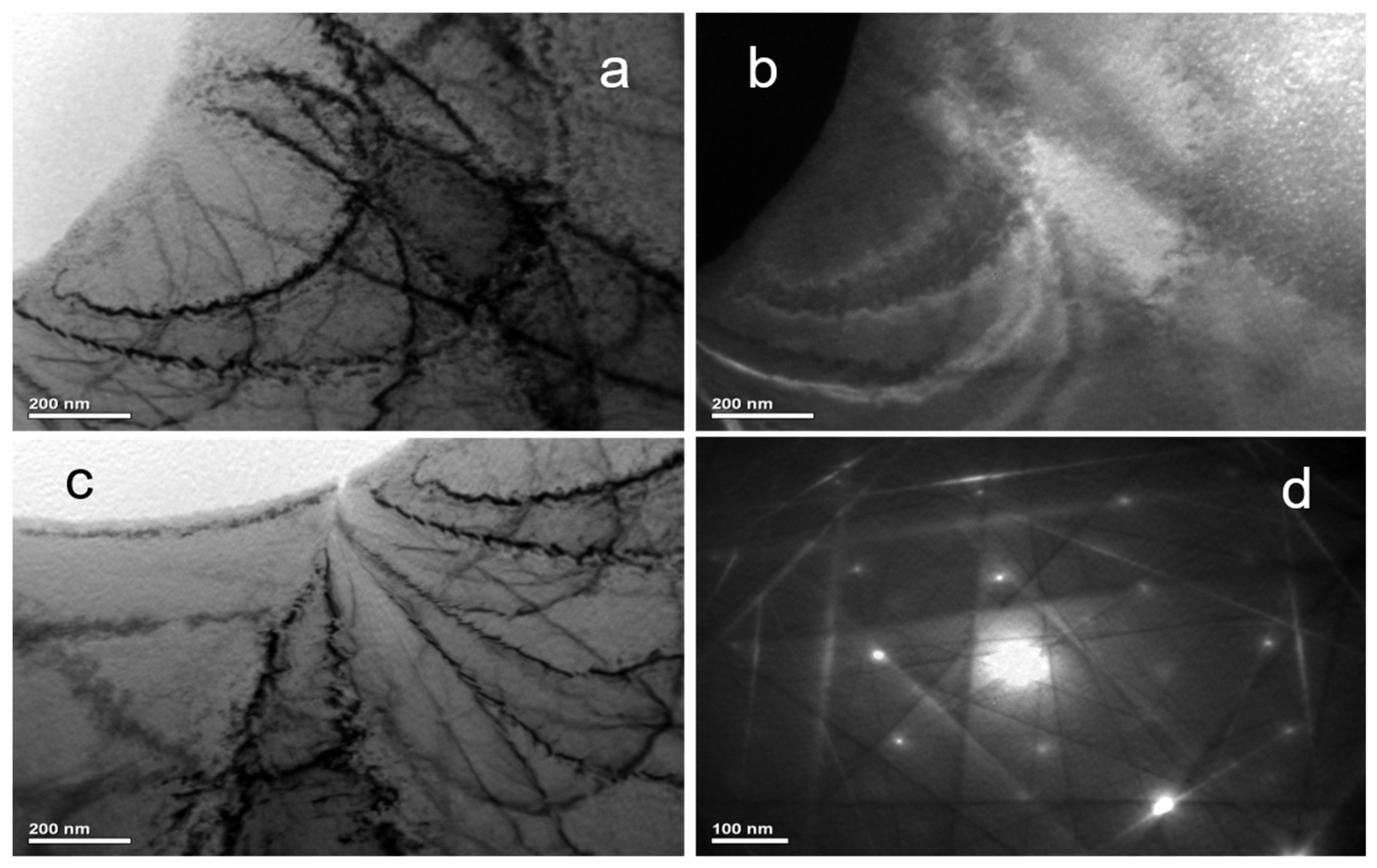
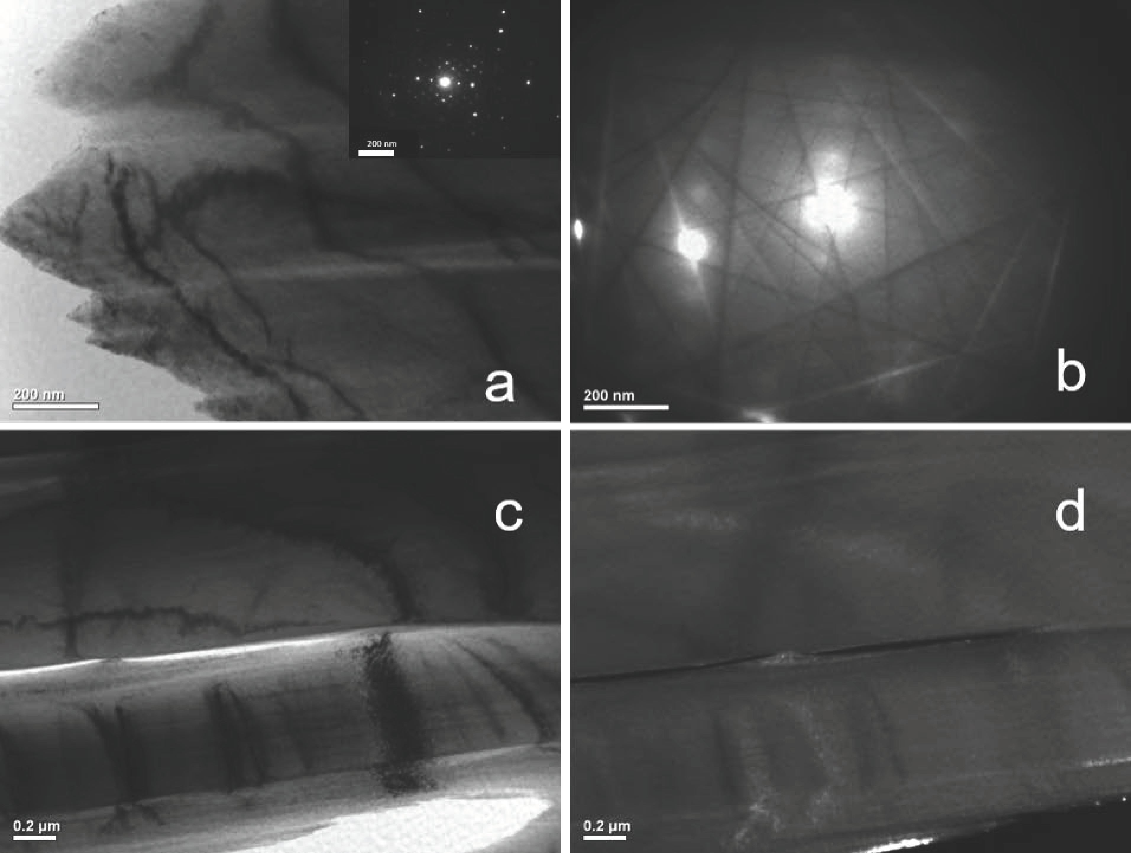
These results were attributed to the microstructure of the used electric steels. Transmission electron microscopy (TEM) studies illustrated that as-cast electric steel offered dislocation density in the order of 108 cm−2, while thermal treatment reduced dislocation density in the order of 105 cm−2, as illustrated in Figure 2 and Figure 3, respectively. The actual thermal treatment was 380 °C in inert atmosphere (Ar) for one hour, followed by a 24 h slow-rate cooling process. Thus, it became important to use thermally treated electric steels.
The shielding arrangement was chosen to be single layer, double layer and multilayer shielding, with the distance between the different layers being controllable and tailored to the needs of the shielding process. Single layer offers an easy manufacturing method, but the shielding response should be expected to be relatively poor. The double and multiple shielding may offer a higher level of shielding at the cost of a relatively more difficult and expensive manufacturing process.
Regarding the parametric response/behavior of such a shielding process, taking into account the distance from the current source, the geometrical details of each arrangement were the subject of the theoretical studies of this paper implementing finite element analysis for the magnetic field distribution calculation, as well as the calculation of shielding effects and experimental studies, by means of monitoring the magnetic field distribution and shielding effects using proper magnetometers.
3. Finite Element Analysis
The main target of this work is to prove that finite element analysis is an appropriate tool for the design of proper shielding conditions against low-frequency electromagnetic fields. The working environment was chosen to be ANSYS Maxwell 2D and 3D, Release 17.1 Academic.
ANSYS Maxwell is a high-output interactive software utilizing finite element analysis to interpret electric and magnetic field problems. This software solves electromagnetic field problems of a known model according to materials, limits and source conditions using Maxwell equations over a limited space region. The Magnetic Field Eddy Current solver was used for our problem: it estimates the oscillating magnetic field, which appears in a specified region due to AC current distribution. Furthermore, all eddy current effects are taken into consideration (involving skin effects) during the calculation of the current densities. This solver calculates the magnetic fields at a specified sinusoidal frequency. Both linear and nonlinear (for saturation effects) magnetic materials can be used. Moreover, eddy, skin and proximity effects are considered. In order to obtain the set of algebraic equations to be solved, the geometry of the area under simulation is discretized automatically into small elements (e.g., triangles in 2D). All model solids are meshed automatically by the mesher, since the Maxwell routine itself offers an optimum adaptation of the mesh. The desired field in each element is approximated with a second-order quadratic polynomial to increase the accuracy of the simulation:
Az(x,y) = ao + a1x + a2y + a3x2 + a4xy + a5y2
Field quantities are calculated for six points (three corners and three midpoints) in 2D. The time step methodology was not applied, since it has a negligible effect in the eddy current solver; usually, it is used in the transient solver. The equations solved were the Maxwell equations in complex form, while the boundary conditions were determined as infinite.
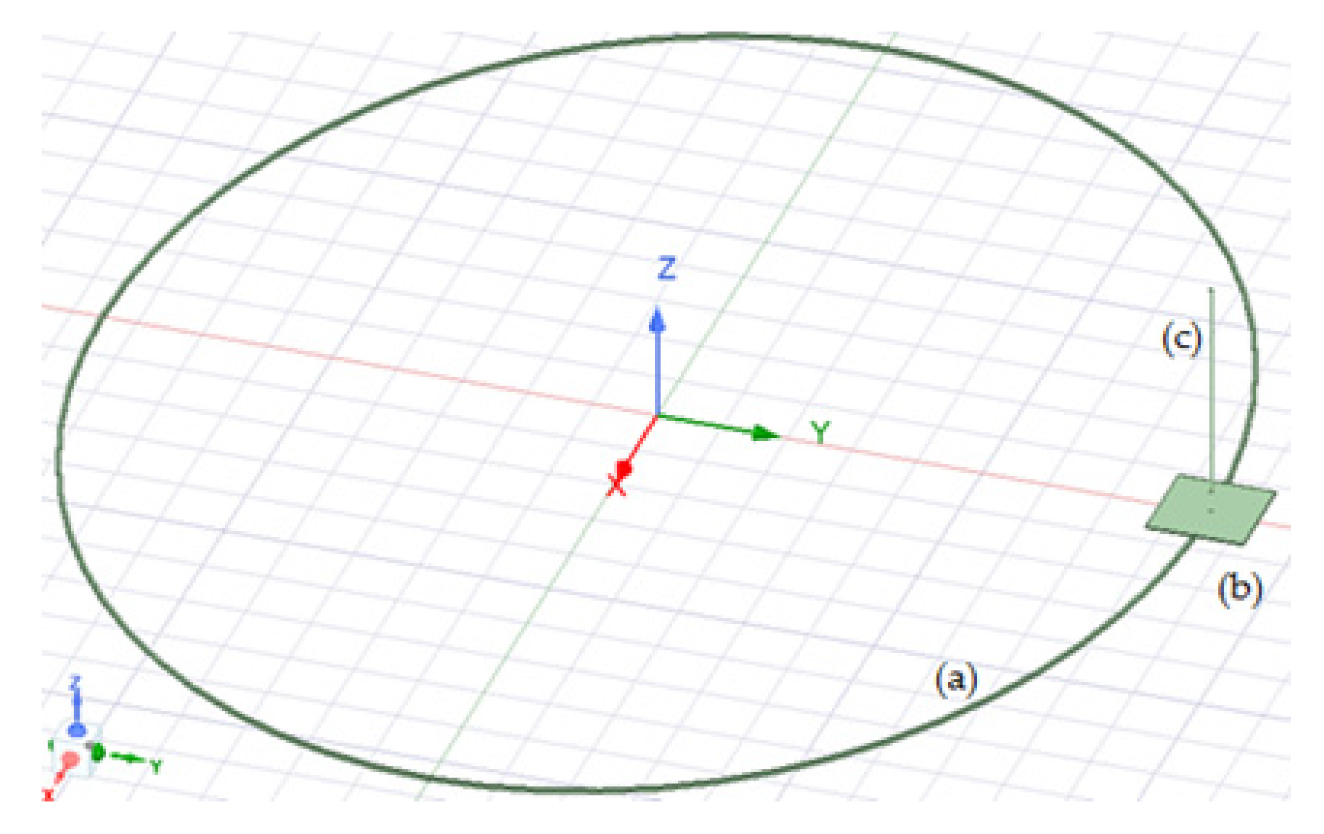
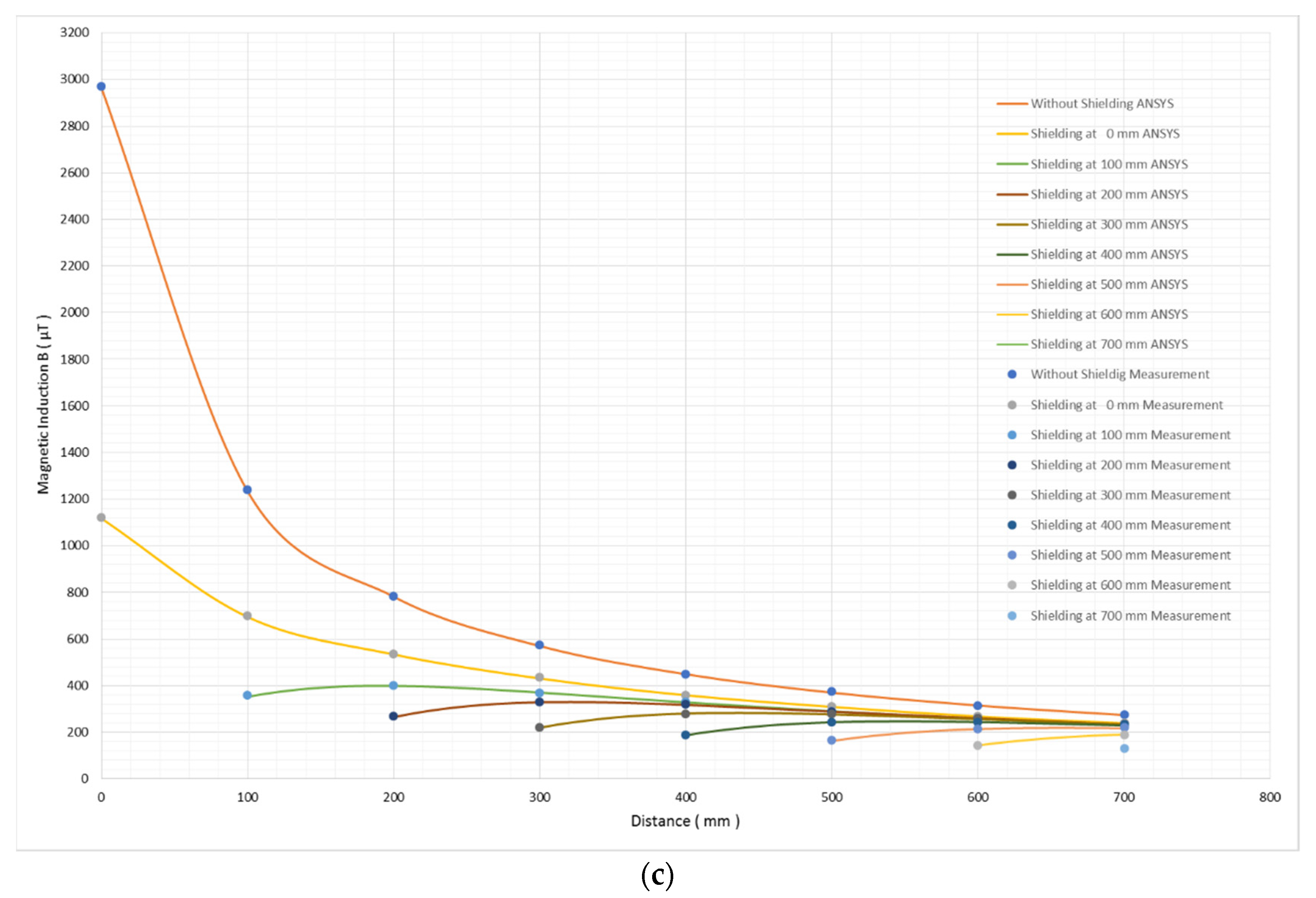
The simulation was realized for a long circular current conductor, fed by a 50 Hz current from 100 to 1200 A. At a given point, a short electric steel rectangle of 30 × 30 cm with a thickness of 0.2 mm was used to shield the electromagnetic field from the circular current conductor. The short electric steel rectangle was set at distances from 0 cm up to 80 cm from the current conductor, while the magnetic field was monitored above the rectangle at distances from 0 cm up to 80 cm. Apart from the single rectangle electric steel sheet, a double electric steel sandwich was also implemented, where the distance between the two electric rectangles was 38 and 100 mm. The schematic used by ANSYS is illustrated in Figure 4.
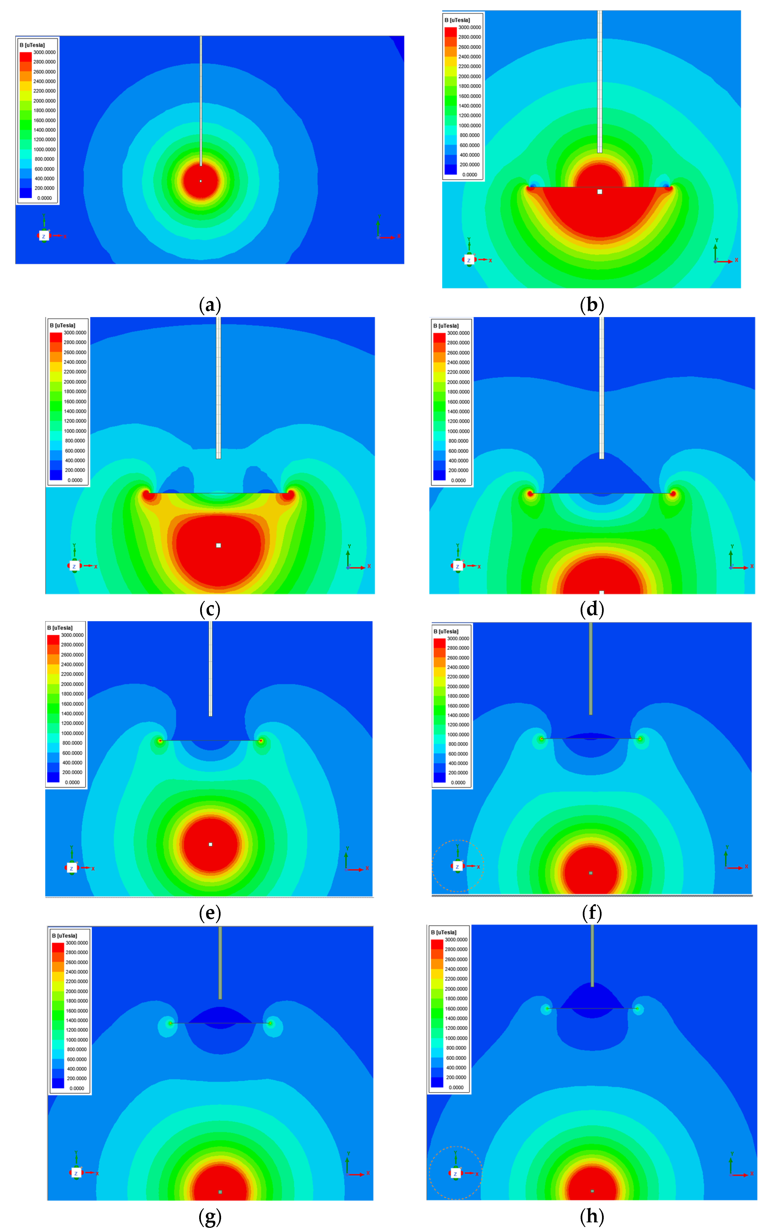
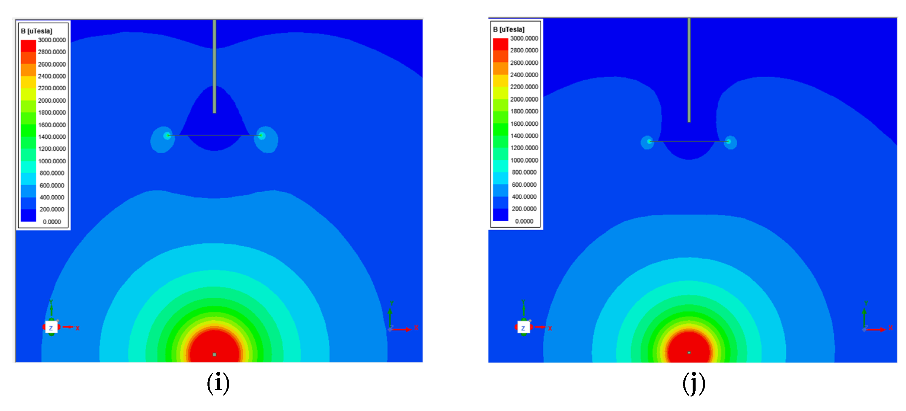
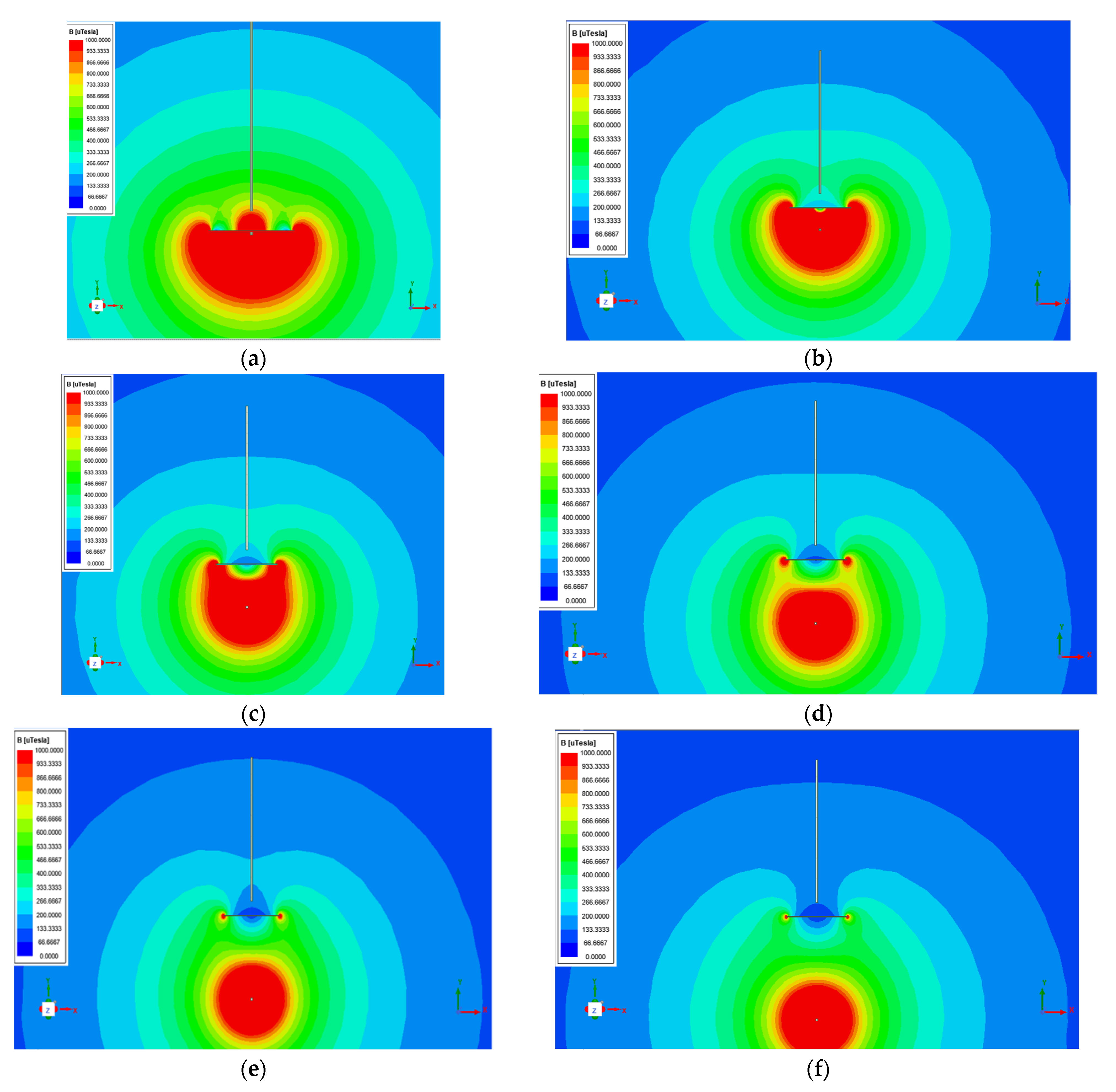
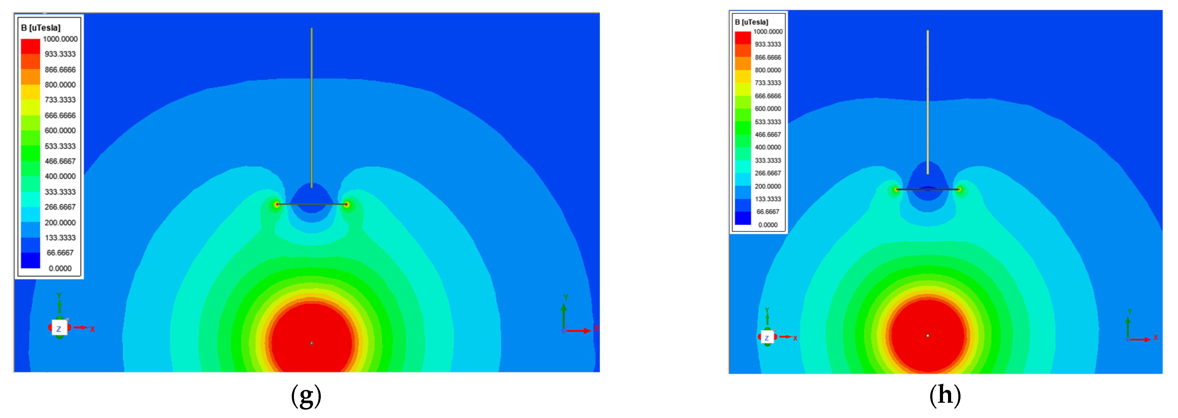
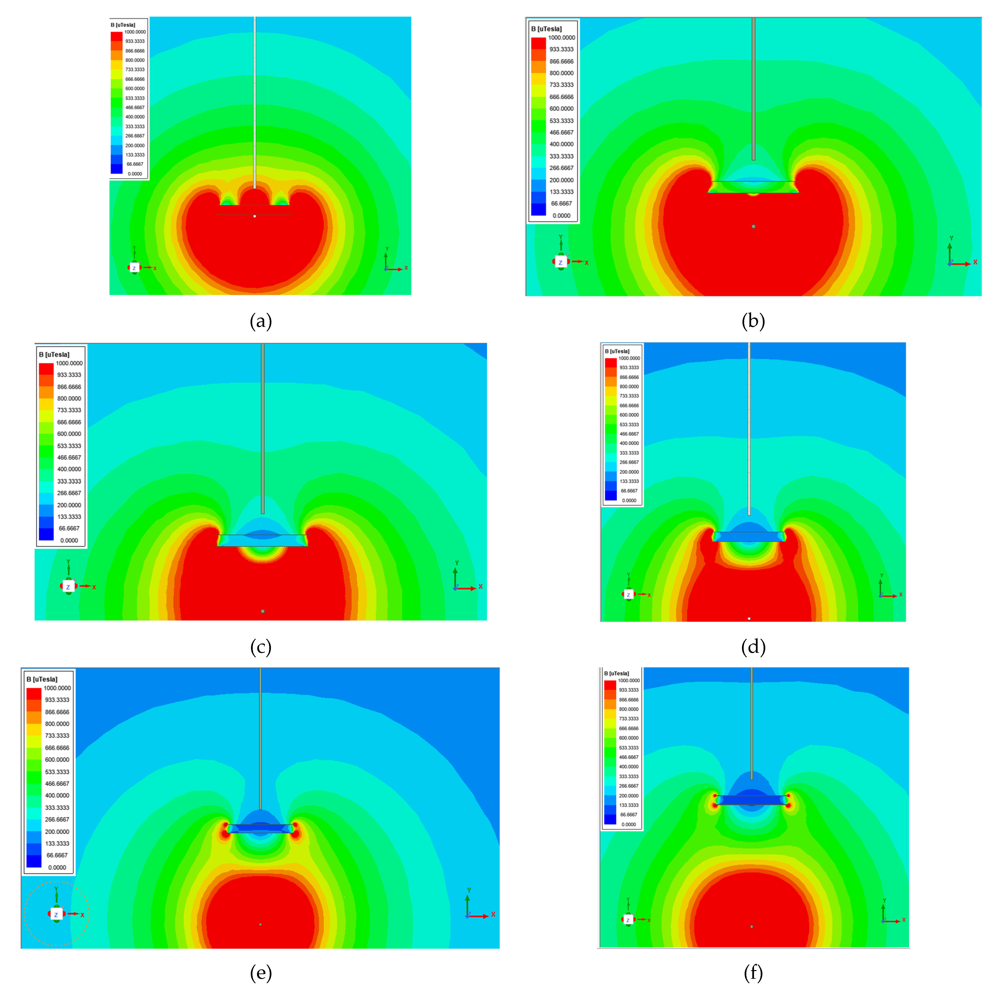
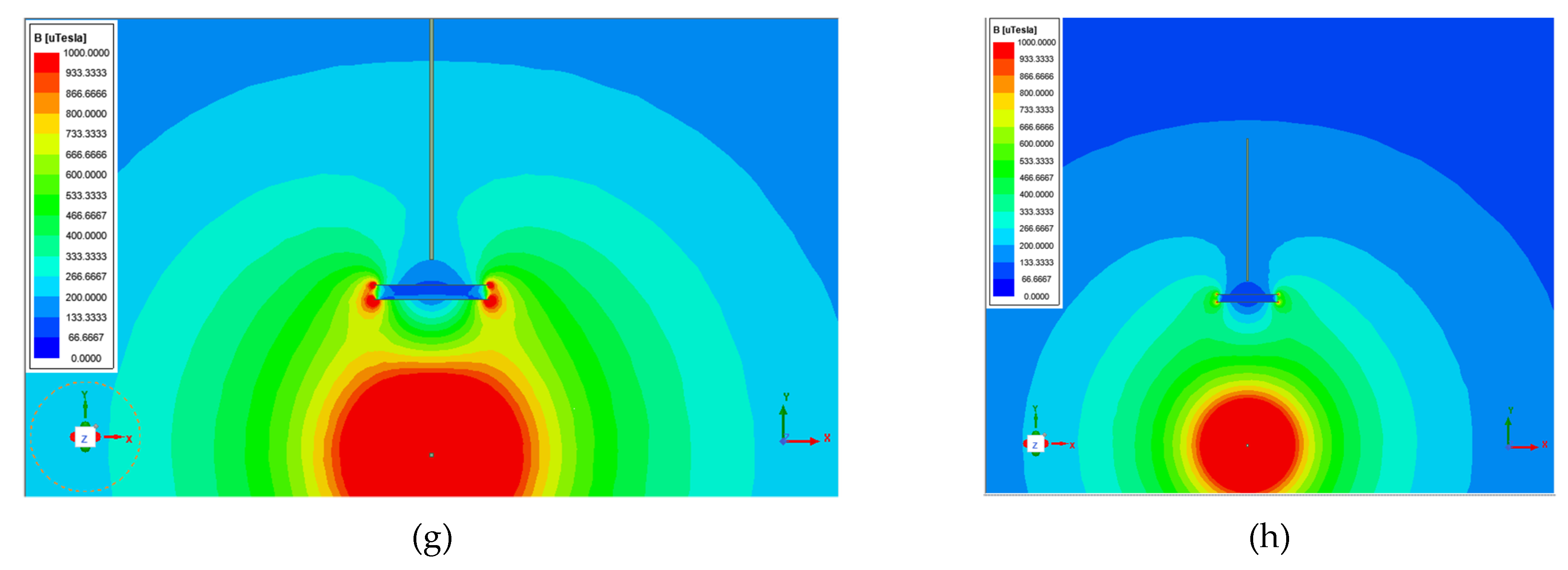
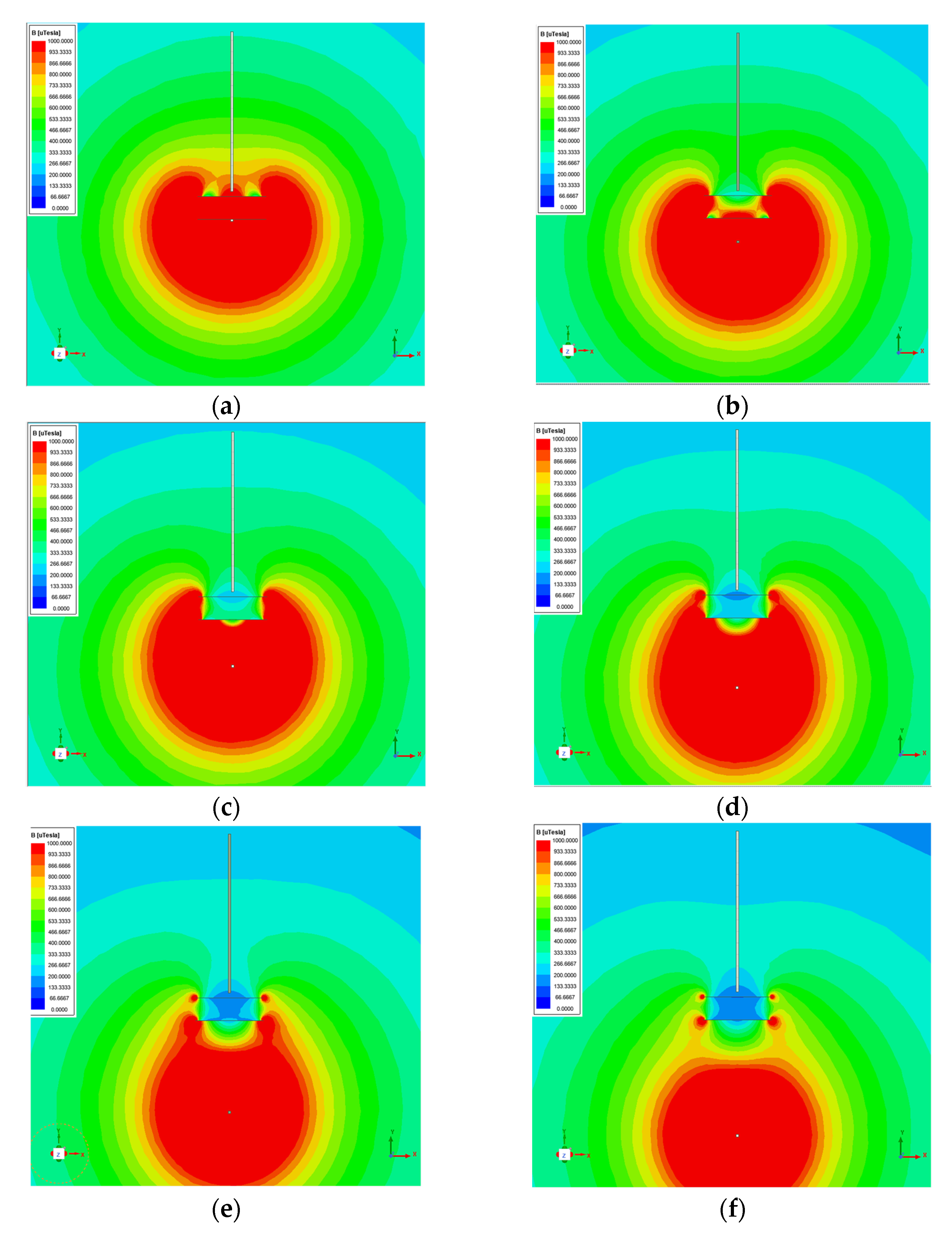
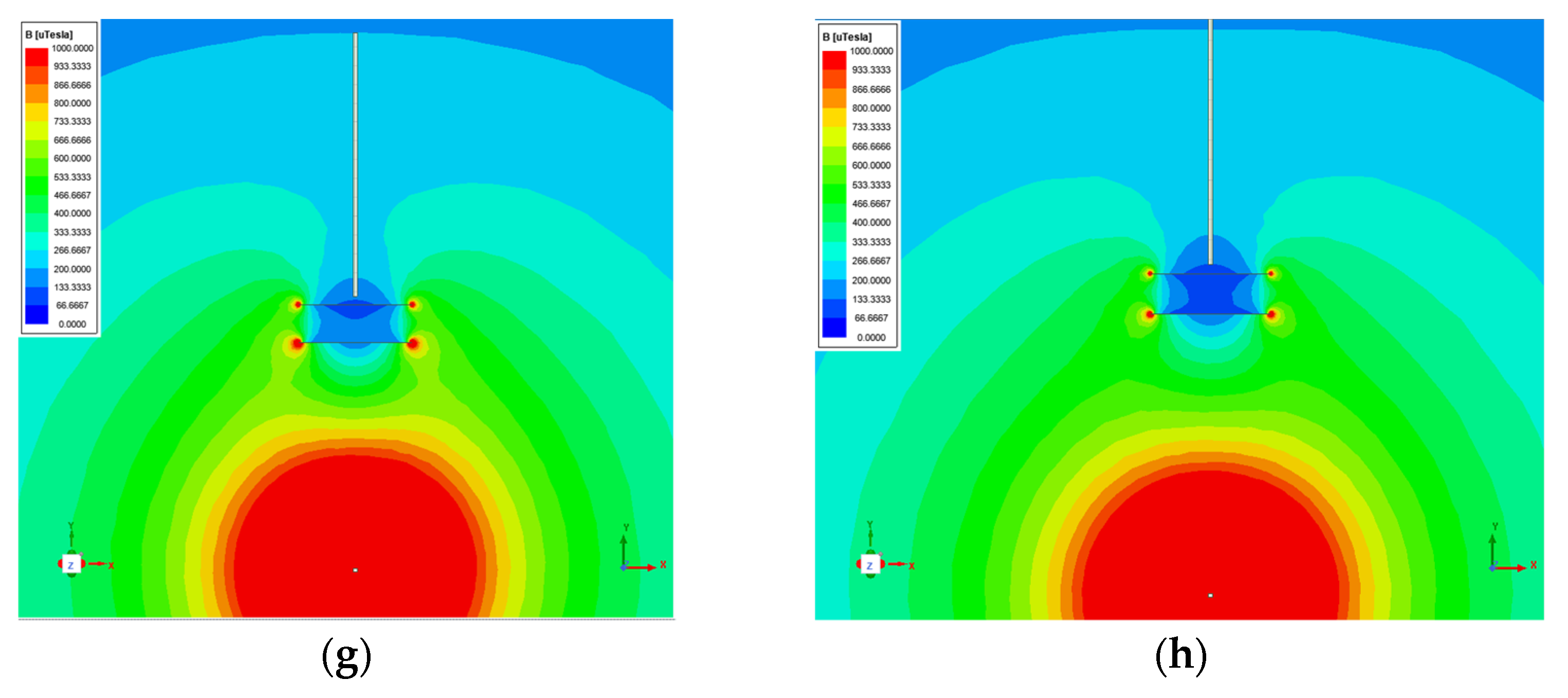
The simulation of the magnetic field as a function of the distance from the surface of the circular current conductor is illustrated in Figure 5a. Figure 5b–h illustrate the calculated field distribution in space for a single electric steel rectangle at 0, 100, 200, 300, 400, 500, 600, 700 and 800 mm distances from the current conductor for a 786 A current. Figure 6 illustrates the calculated field distribution in space for a two-layer sandwiched electric steel rectangle of 5 mm distance between shielding layers at 0, 100, 200, 300, 400, 500, 600 and 700 mm distances from the current conductor for a 577 A current. Figure 7 illustrates the calculated field distribution in space for a two-layer sandwiched electric steel rectangle of 38 mm distance between shielding layers at 0, 100, 200, 300, 400, 500, 600 and 700 mm distances from the current conductor for a 777 A current. Figure 8 illustrates the calculated field distribution in space for a two-layer sandwiched electric steel rectangle of 100 mm distance between shielding layers at 0, 100, 200, 300, 400, 500, 600 and 700 mm distances from the current conductor for a 1055 A current. Note that simulation results for more current levels are also available, and they will be included in future works.
It can be seen that the dependence of the magnetic field on the distance from the shielding electric steel is not monotonic. This is due to the trapping of magnetic lines from both sides of the magnetic materialfield. Thus, the field distribution at the outer part of the electric steel sheet decreases up to a point that magnetic lines are driven to be trapped by the electric steel sheet, whereas above this, the contribution of the magnetic field from the whole conductor offers an increase in the field distribution.
The main proof of the validity of the simulation process is the comparison of these simulation results with the corresponding experimental results, illustrated in the next chapter.
4. Experiments
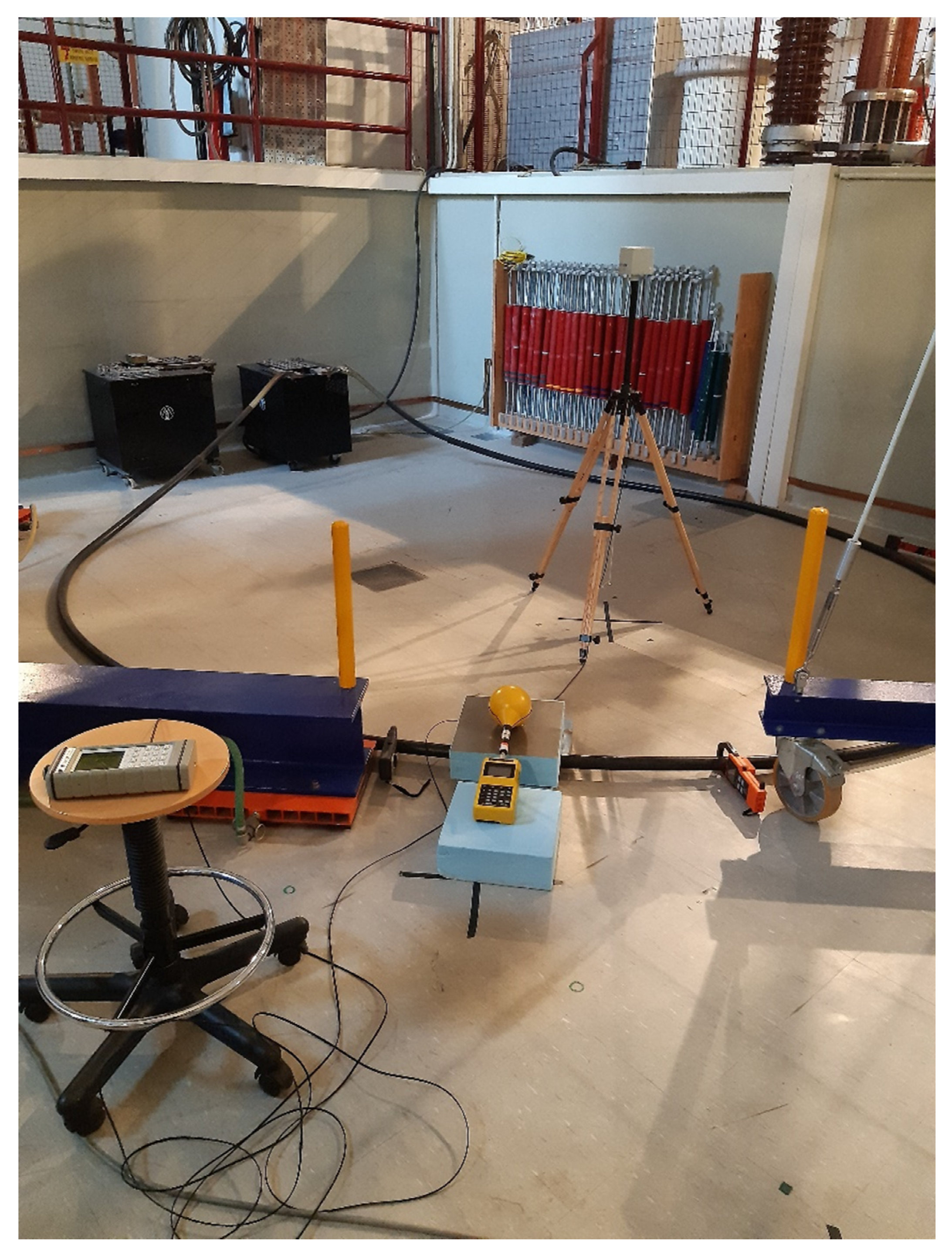
Figure 9 depicts the experimental set-up used for the evaluation of the finite element analysis simulation. The experimental process followed the theoretical studies/calculations of the magnetic field. A current transformer (CT) with a range of 0–6000 A was used to provide the required value of the current (500 to 1100 A). A medium voltage cable (MVC) (1 × 240 mm2) was connected to the secondary side of the transformer. The variation of the produced current was controlled by a variac (VC), which was connected between the low-voltage network and the primary of the transformer. The current of the cable was measured during each cycle of measurements with a calibrated clamp meter (CM). The variation of the current was less than ±0.5% during each measurement. The magnetic field generated by the medium voltage cable was measured with a suitable sensor (BS) and a field meter (FM).
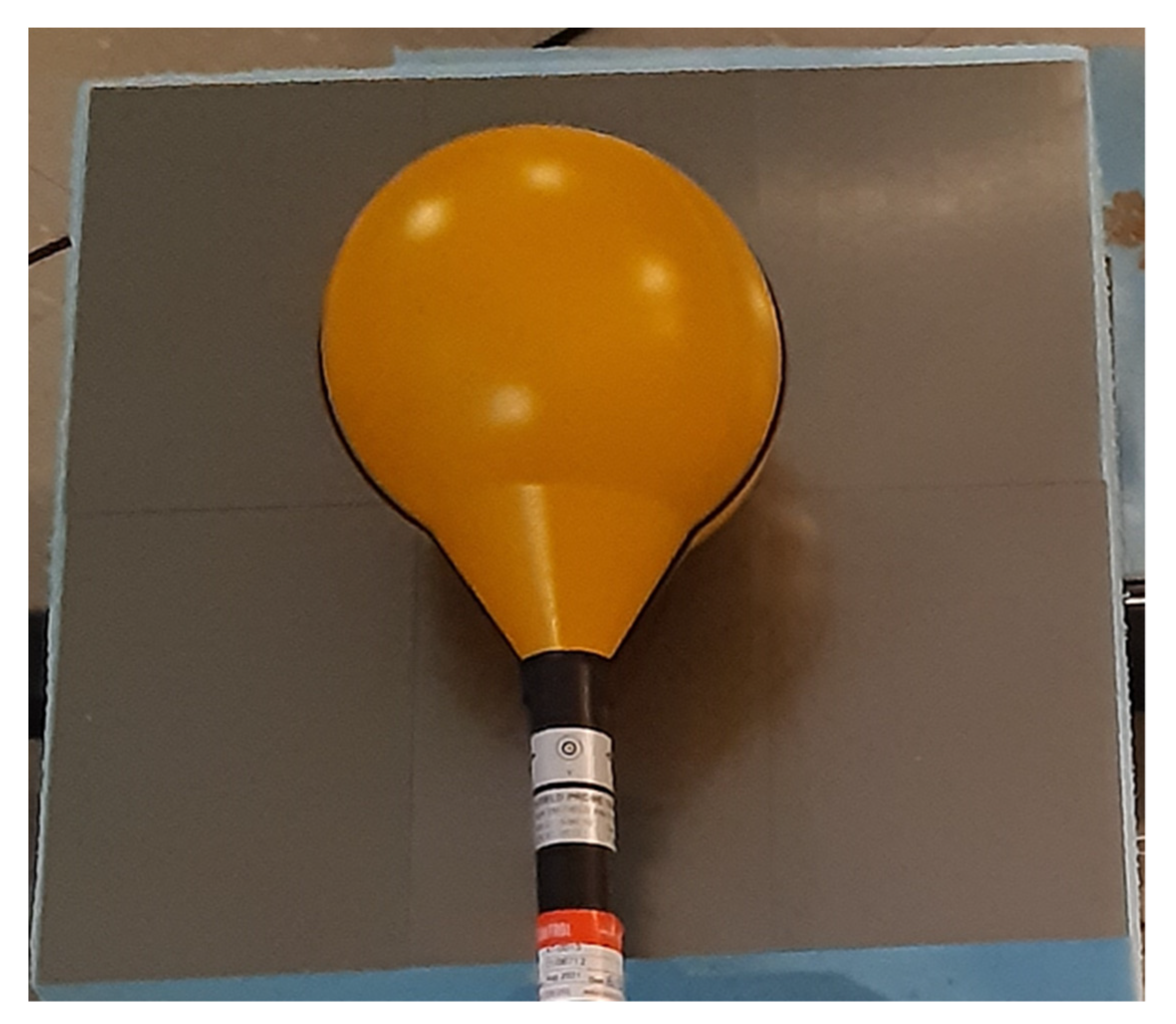
The 30 × 30 cm single and double electric steel layers were composed of six orthogonal pieces with a width and length of 10 and 15 cm, respectively (Figure 10). In the same figure, the testing field meter is also illustrated. The field meter (FM1) with the suitable sensor (BS1) (NARDA/EFA 300 with 100 cm2 probe) was calibrated at 2021, offering a typical uncertainty less than ±3%. The main parameters of the uncertainty were the accuracy of the field sensor, the variation of the injected current, the repeatability and the non-uniform magnetic field. During the measurements, the temperature was 22 °C ± 1 °C, and the relative humidity was 44% ± 4%. The sensor operated in the magnetic mode. The minimum distance of the sensor from the conductive surface was less than 1 mm. However, the sensor sensing surface was as large as several cm. Therefore, it averaged out the field within the sensing surface, which was vertical to the surface of the soft magnetic sheet.
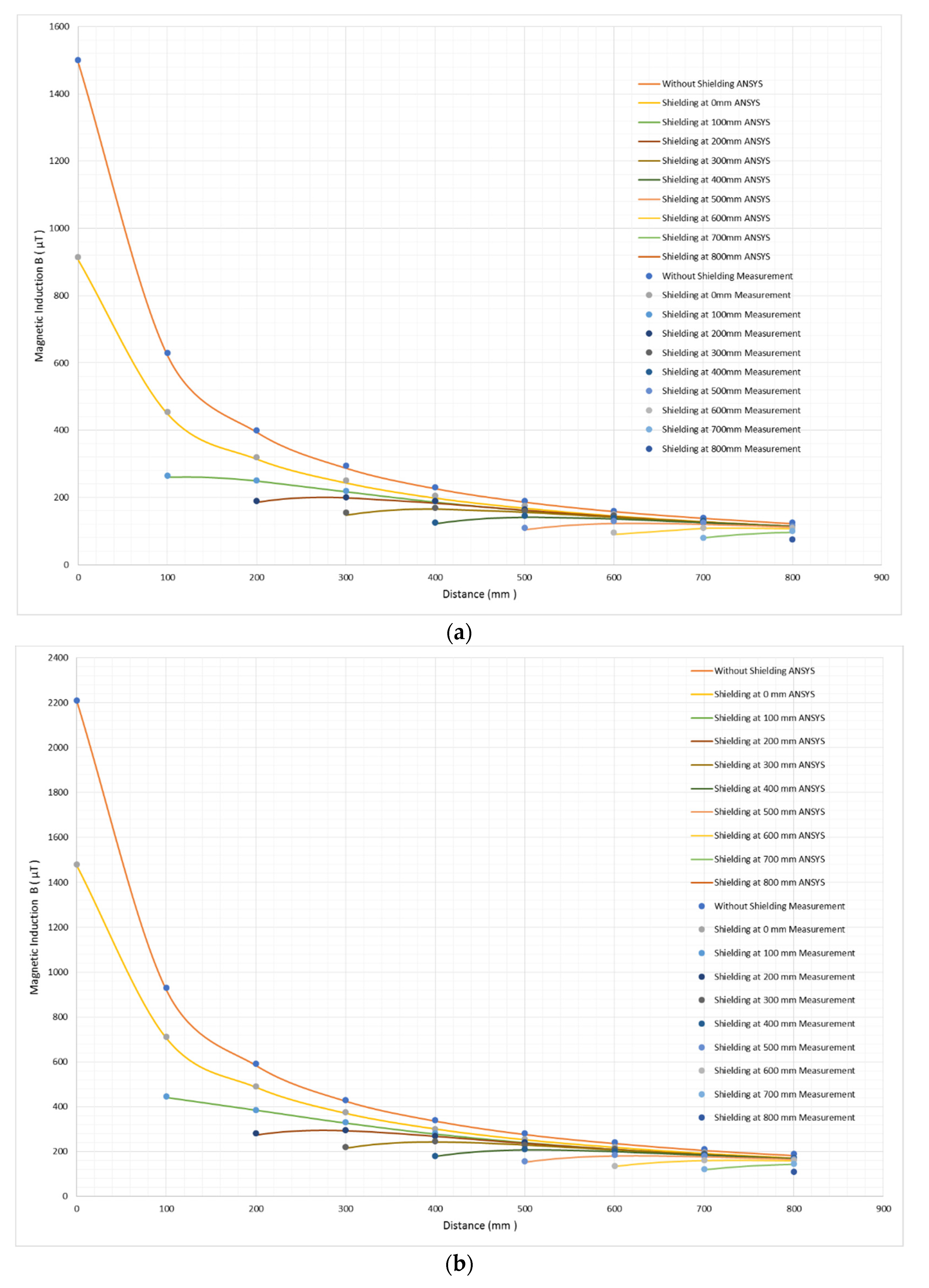
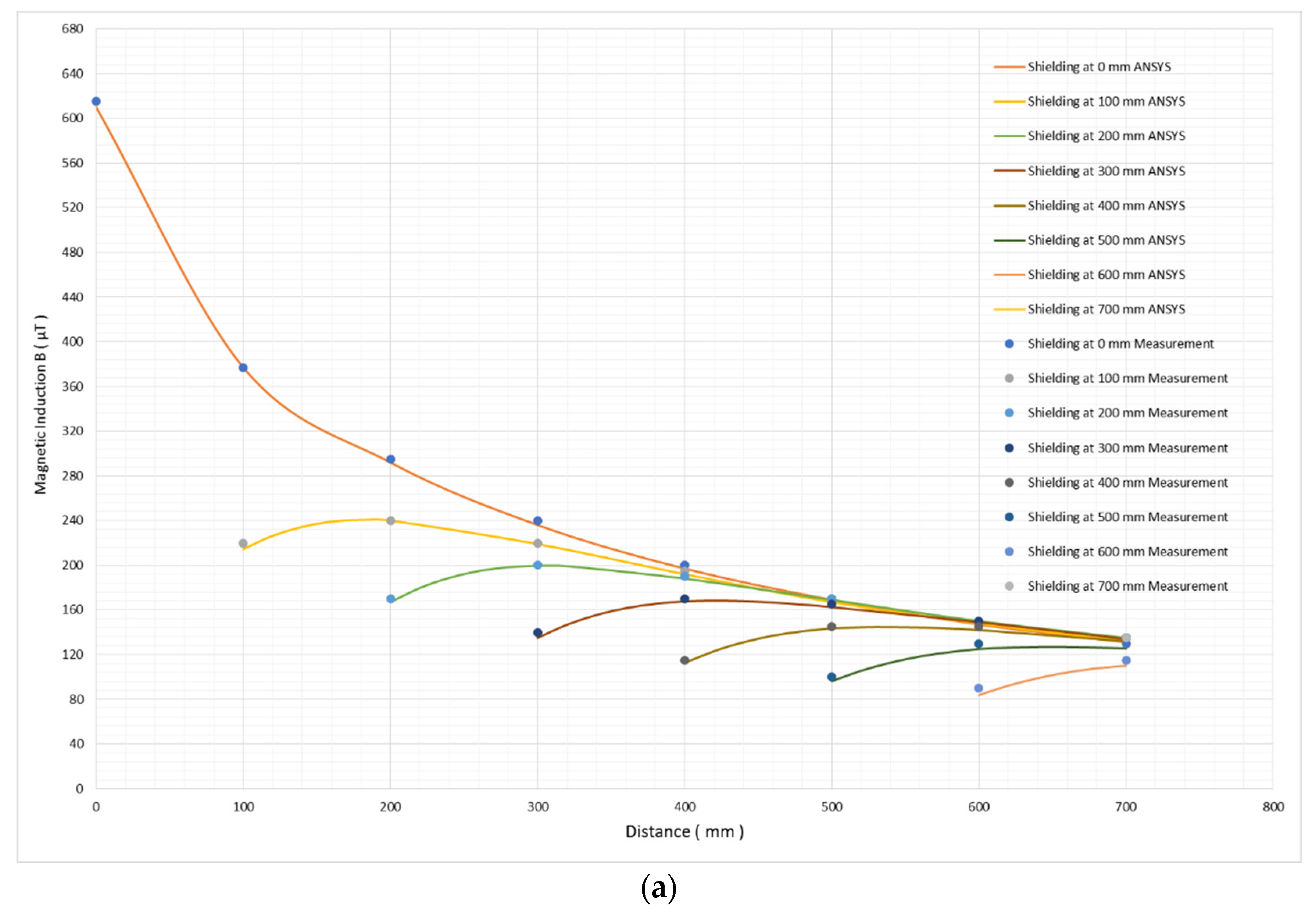
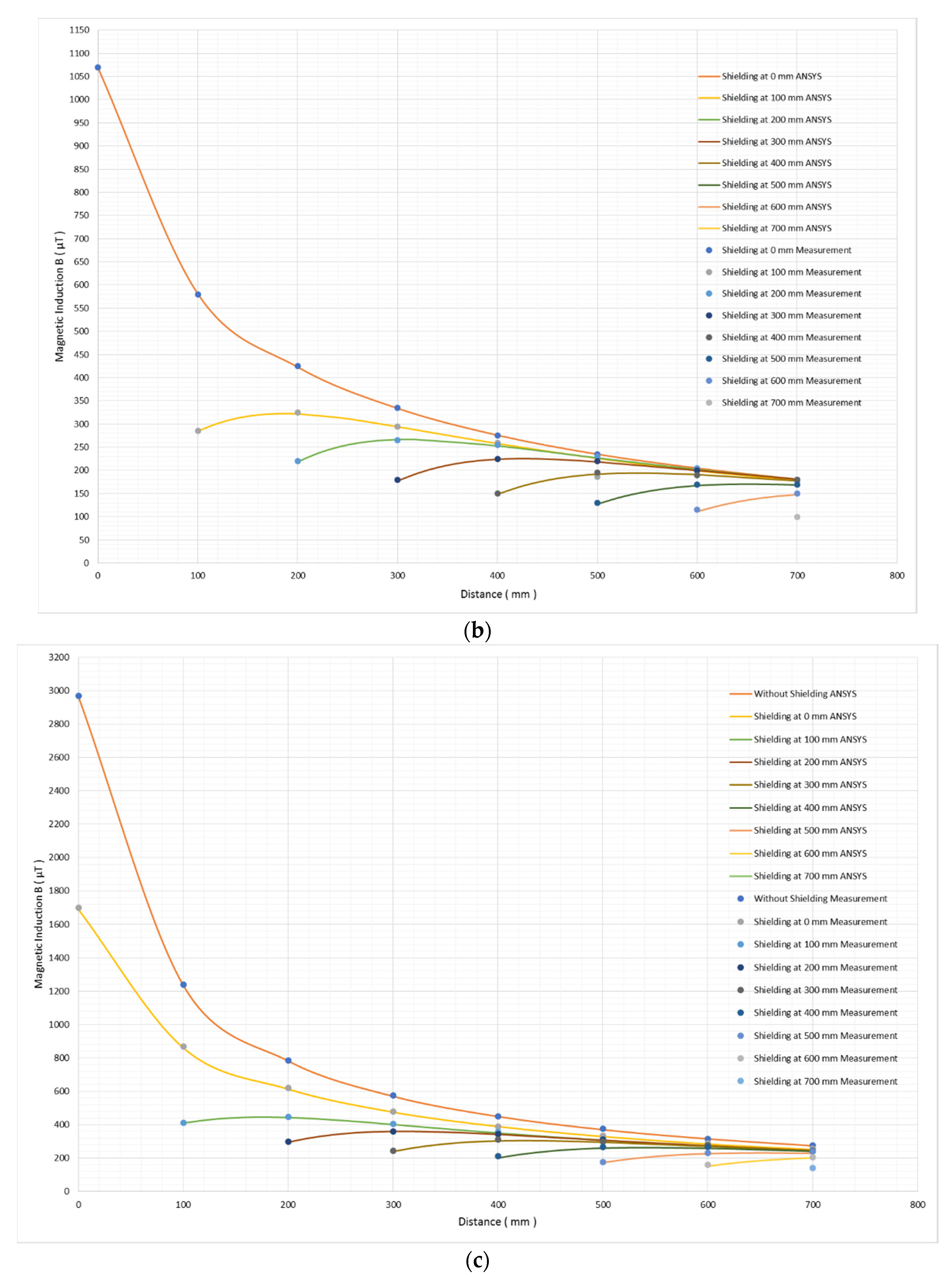
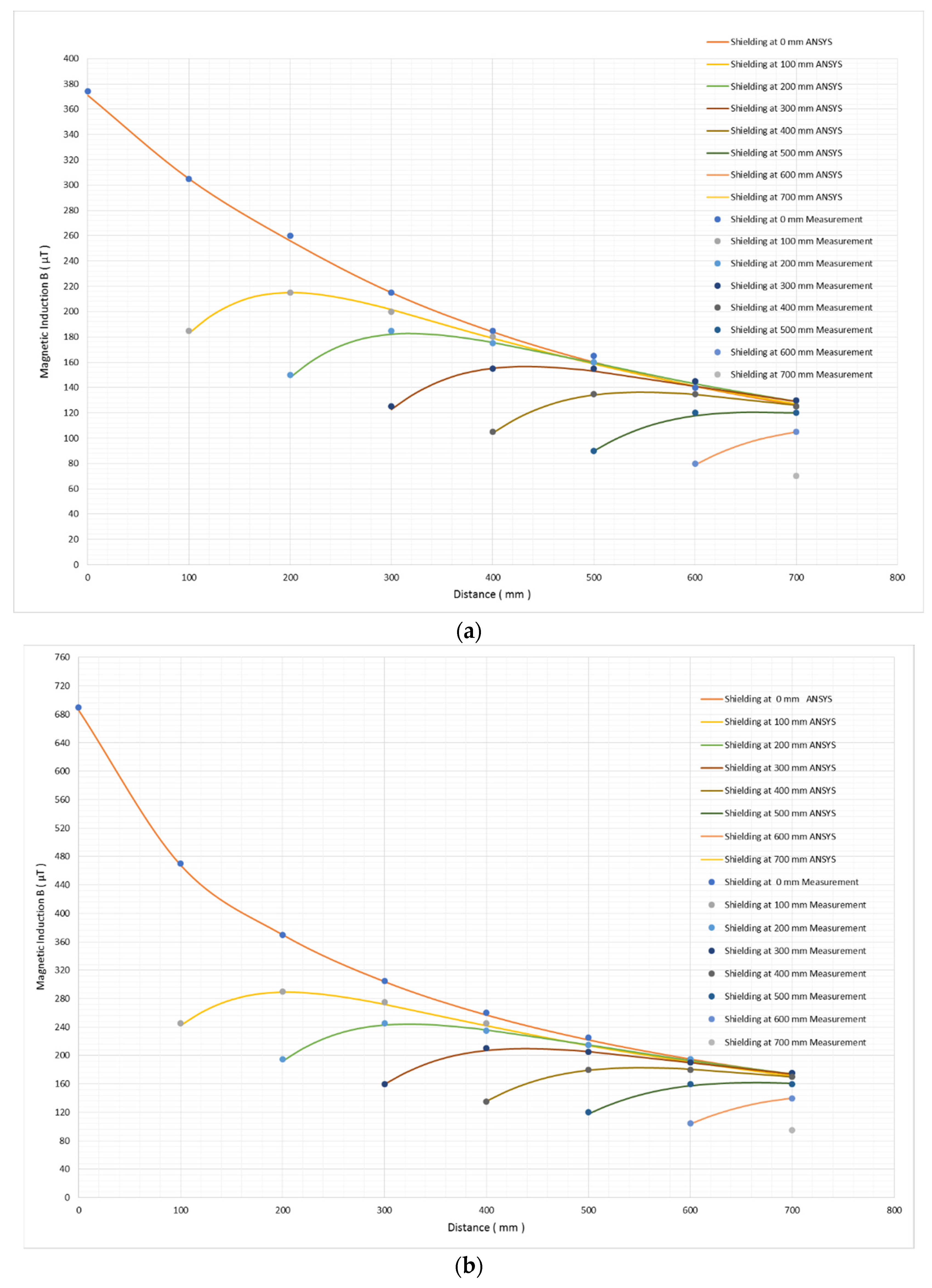
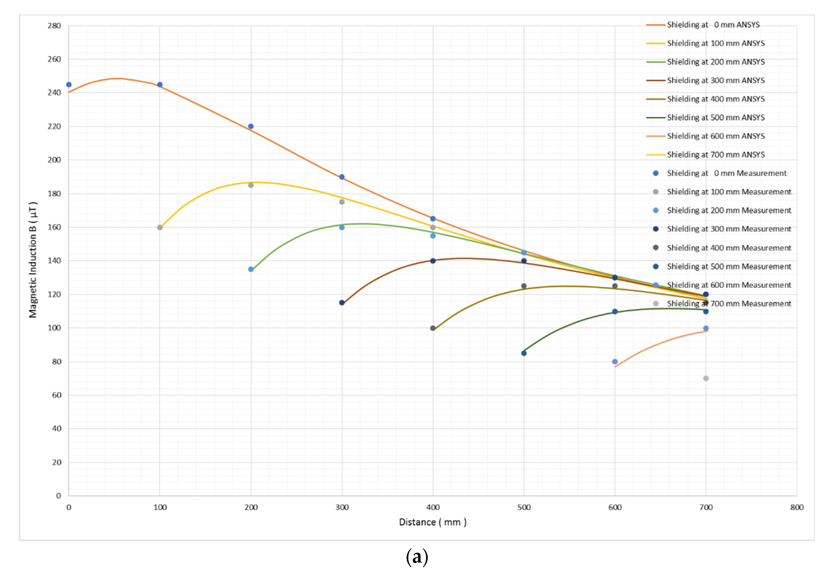
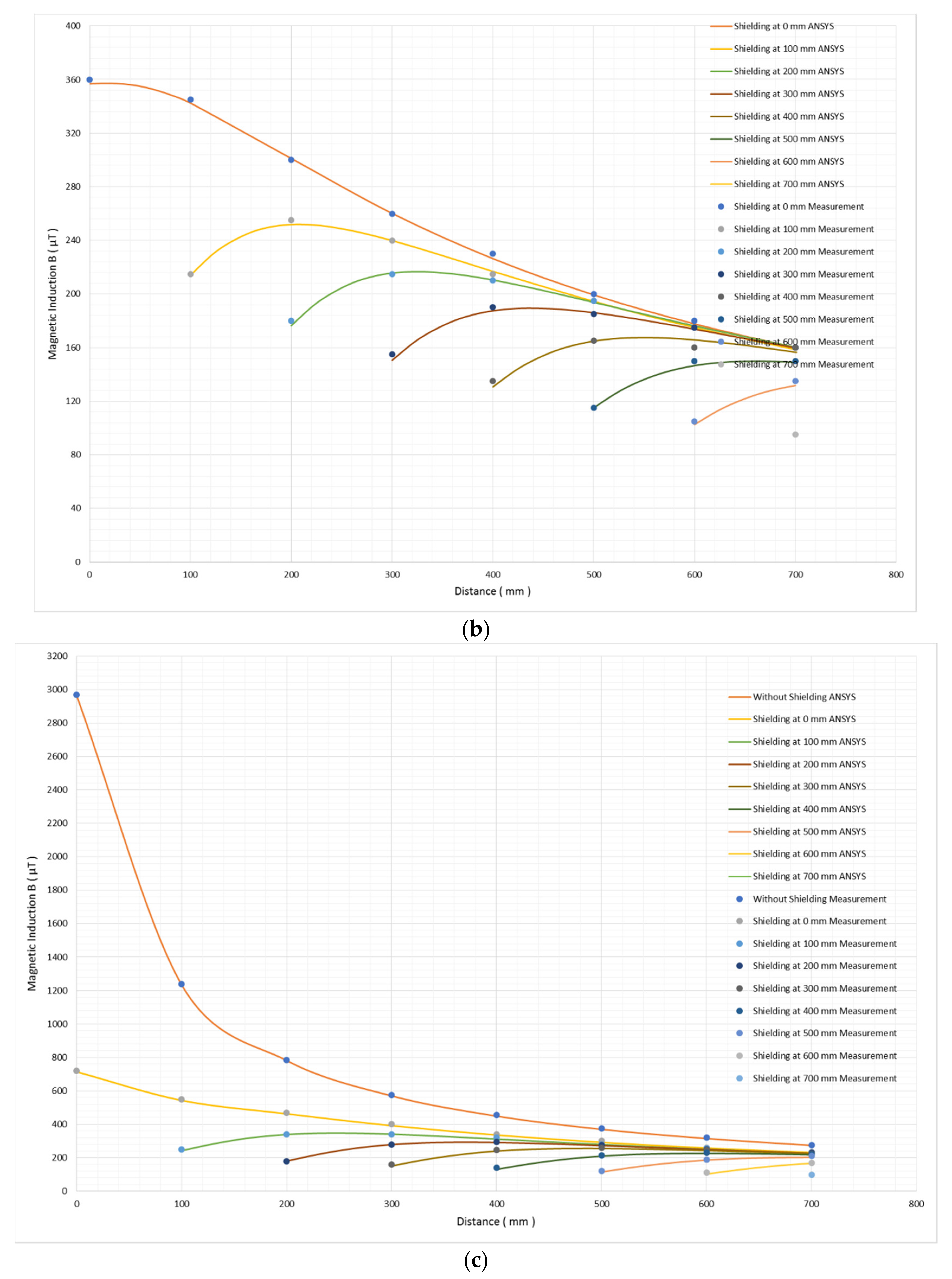
Figure 11 illustrates the measured and calculated field distribution in space for a single electric steel rectangle set at 0, 100, 200, 300, 400, 500, 600 and 700 mm from the current conductor. Figure 12, Figure 13 and Figure 14 represent the measured and calculated field distributions in space for two-layer sandwiched electric steel rectangles separated at 5, 37 and 100 mm, respectively, at a 0, 100, 200, 300, 400, 500, 600 and 700 mm distance from the current conductor. In these figures, the agreement between the FEA calculated values and the experimental results is qualitatively clear. No fitting of the experimental results was tried, since the purpose of the comparison was the agreement between the calculated and experimental results: the clear agreement between the experiments and calculations permits the use of FEA based on the ANSYS codes to design, calculate and predict the shielding effect of given highly permeable magnetic steels. Importantly, the same non-monotonic dependence of the field on the distance was observed in both the calculated field values and the experimental results. The explanation of the non-monotonic response is the field trapping in the vicinity of the highly permeable magnetic sheet: magnetic lines are trapped in the magnetically soft sheet, and, therefore, the field is reduced in its vicinity. In order to determine the uncertainty and the error of the measurements, the total uncertainty of the measurements was determined. Such uncertainty is due to the following:
- The uncertainty of the sensor: the combined standard uncertainty was determined to be 3.09% at its latest calibration.
- The uncertainty of current supply: the monitored maximum uncertainty of the current transmission was determined to be 3 A per 1 kA, resulting in 0.3% uncertainty. Taking into account the uncertainty of the Ammeter, which was determined to be 1.5% at its latest calibration, the total uncertainty due to current transmission was 1.8%.
- The uncertainty of the position of the shielding material and the uncertainty of the positioning of the magnetic field sensor. Each one of these uncertainties was determined to be 1 mm in a range of 10 cm (100 mm), resulting in a relative uncertainty misplacement of 2%.
Thus, the total estimated uncertainty of the measurements was determined to be 6.89%. Note that the sources of the uncertainty of the magnetic field taken into account for the analysis were described in Annex C and Table D.1 of the standard IEC 61786-2:2014 [21].
The average deviation between the experimental data and the calculated field values was determined to be 7.2%, which seems to be reasonable within the limits of the experimental set-up. However, a maximum deviation of 9.5% between the experimental and calculated results was determined, particularly in the case of the close placement of the shielding material to the current conductor. This large deviation is attributed to the mechanical vibrations of the electric steel sheets contributing to the response of the magnetometer.
These measurements and their agreement with the calculated field values are the actual proof that the ANSYS finite element analysis is sufficiently appropriate for the calculation of the magnetic field in the given conditions of shielding. Thus, the ANSYS finite element analysis can be considered as a trustful shielding design tool.
5. Discussion
The results, obtained from both the simulation and experimental works, illustrate that the proposed methodology for designing the shielding process by finite element analysis provides accurate results, as it is certified by the qualitative and quantitative agreement between the simulation and experiments. The most profound result was the prediction of the non-monotonic dependence of the magnetic field on the distance from the surface of the shielding electric steel sheet. Quantitative disagreements are due to the actual level of residual stresses of the used electric steel sheets, as well as the fact that the electric steel sheet was made from pre-cut pieces of electric steel instead of a continuous sheet. However, there was no experimental and simulation result where the two curves crossed over each other, thus suggesting that finite element analysis was proven to be a trustful tool for the design of the proper shielding system.
It is suggested that the thin magnetic shielding sheets are placed together with aluminum sheets for two reasons: the first one is to avoid the stretching of the magnetic sheets, which would decrease their magnetic permeability; the second reason is the additional eddy current-based shielding in high frequencies, offered by the aluminum sheets.
The experimental and the simulation processes reveal that the best conditions for a low-frequency electromagnetic field are achieved by a double layer of electric steel sheets, even if these sheets are pieces or ribbons of steel arranged in a way to simulate a continuous shielding surface. The distance between the two shielding layers appeared to not be so important, with a small optimum presentence of the case of the 100 mm distance between the two shielding layers. However, such a distance is pretty large, not allowing for universal application.
Furthermore, the simulation and experimental works were restricted to a single-phase excitation and not a three-phase one. Concerning three-phase excitation, the effective field interference may be rather smaller because of the averaging due to the 120 o phase shift of the three phases. However, in cases of close vicinity between the area that needs shielding and the power transmission lines, especially in the case of 400 kV, the distance between consequent power lines is about 7.5 m, thus requiring single transmission line behavior for shielding between consequent phases just below the transmission lines. In addition, it is safe to design field shielding for single-phase transmission lines in order to avoid problems in case of phase failure.
Therefore, the proper algorithm to obtain the optimum shielding for low-frequency fields is the following:
- First, the area to be shielded has to be designed with respect to the power transmission lines.
- Consequently, the shielding structure has to be arranged with respect to the surface(s) closer to the power transmission lines. Such shielding has to have a double layer with an in-between distance from 10 to 100 mm. Actually, the shielding based on electric steel sheets can be based on thermal insulating foams (polyurethane etc.), which usually have a thickness from 38 to 100 mm. Note also that those separating foams can also serve as thermal insulating means.
- Then, the finite element analysis illustrates the shielding effect and the minimum distance from the shielding, permitting the presence of human beings (or electronic/electrical instrumentation).
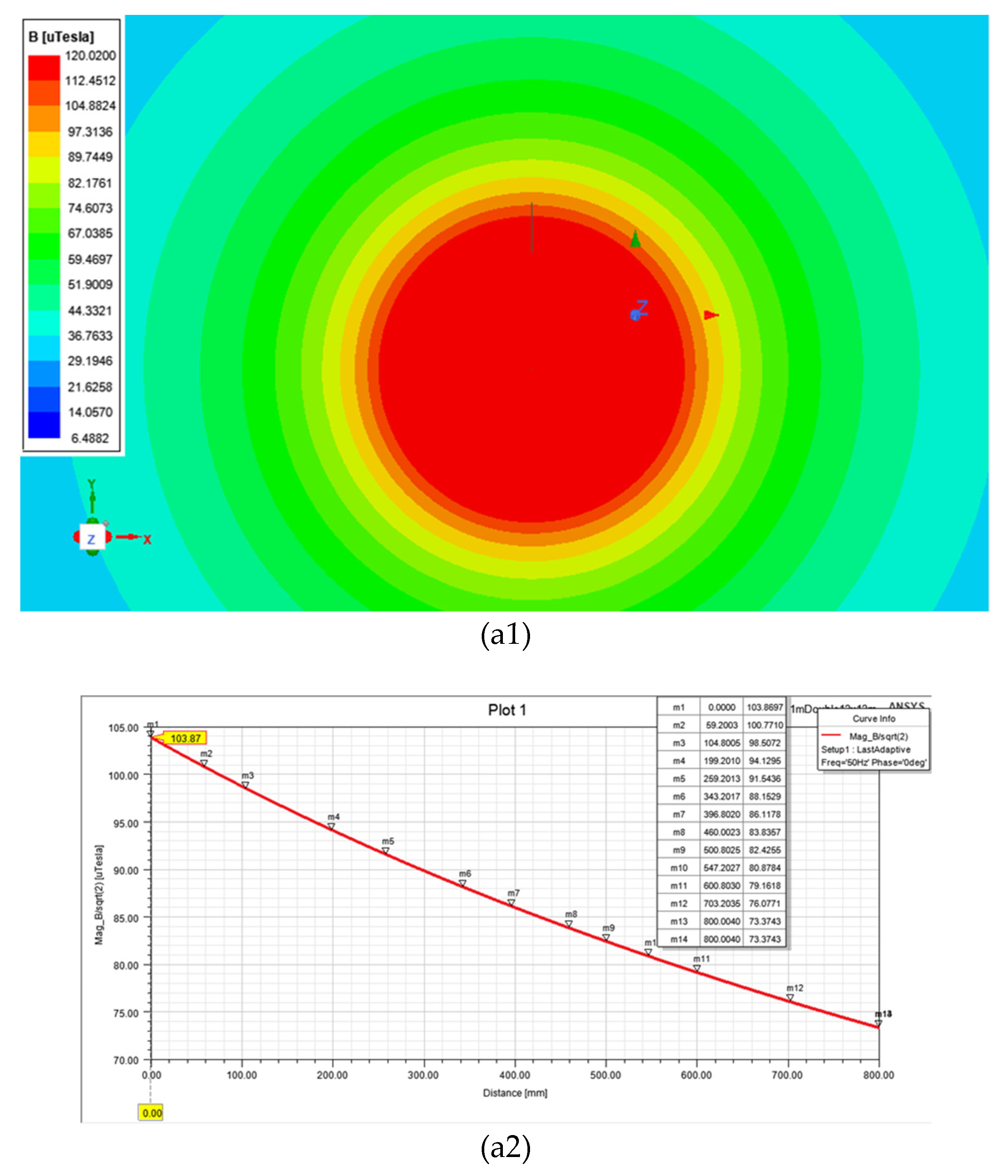
This simple process may enable engineers to design shielding for buildings (houses or working areas) in the vicinity of power transmission lines. As an example, a simulation of the shielding effect concerning a single power line and a flat surface at a 1 m distance from the power line was tried. The closest surface of the building was arranged to be a flat cement surface of 10 m length and width, resulting in a 100 m2 total surface. The actual conditions of electromagnetic interference were that a single power line transmits a field that is shielded by a single or double electric shield sheet layer. In fact, the shielding material comprises electric steel sheets of 0.2 mm thickness, 1500 mm width and length dependent on the actual needs. In other words, the electric steel sheet is offered in the form of steel coil, which covers the surface under the shielding. Figure 15 illustrates the field distribution without shielding, with single and double shielding layer electric steel sheet. Double shielding was simulated for polyurethane of 100 mm thickness. The simulation illustrated that the optimum shielding design refers to the double shielding, as expected. The safe distance from the shielding surface was dependent on the amplitude of the transmitted alternating current. For a 1 kA current, which consists of the most powerful condition, the minimum allowable distance of a human being, in order to experience less than 100 mT field, was 3 m away from the shielded surface, suggesting that it is preferable that such living places should be inhabited 4 m below the power transmission line, provided that the proper (double) shielding means are used. In the case of a single layer shielding means, this distance has to increase to 10 m.
A major issue for the proper operation of the shielding ability of the highly permeable magnetic sheet is the protection against residual stresses, which may affect its shielding ability. Stresses on these soft magnetic sheets may decrease their permeability dramatically. The use of a mechanically soft separation layer between the two magnetic sheets is one prerequisite to ensure the absence of stresses on these magnetic sheets, with the other one being an additional protecting/packaging mechanically soft layer outside the magnetic sheet sandwich. These three stress-protecting layers may be of mechanically soft polymeric foam, such as polyurethane, offering the additional need of thermal insulation.
In addition, bearing in mind the difficulty of using finite element analysis, it is interesting to develop a lighter software application to perform a quite similar simulation process. Any modern application software and language can serve this purpose. As an example, the Python language is referred to as having developed a corresponding routine. Work on such an algorithm is scheduled for a future publication.
Finally, the described shielding method can be used as an inexpensive method of transforming overhead transmission lines to underground ones. This can be realized by excavating surface tunnels in the areas that electric power has to be transmitted, then coating the existing aluminum lines with a proper polymeric coating and placing them in plastic tubes. Then, after filling the tunnel with soil, the single or double layer magnetic shielding is set on top of the soil, before covering it with additional soil. Considering that the electric steel sheets have to demonstrate anticorrosive properties, these electric sheets have to be coated with a proper polymeric coating, practically thicker than the classic micron-thick coating they have from the corresponding manufacturing line. This is actually another scheduled work for a future publication.
6. Conclusions
In the present study, a method for the efficient electromagnetic shielding of high-voltage transmission lines is introduced. The current paper deals with the development of a procedure, based on FEA, for the appropriate design of an efficient passive shielding, using electric or highly permeable sheets. It is worth mentioning that the primary goal of this work is to demonstrate FEA as an efficient tool for the design of proper shielding conditions against low-frequency electromagnetic fields. The computations obtained from the finite element analysis are compared with laboratory measurements in an effort to examine the adequacy of the developed procedure. The good agreement between the theoretical and experimental outcomes establishes the presented methodology as a useful and efficient tool for the design of a proper shielding configuration against low-frequency fields. Indeed, both the qualitative and quantitative convergence between the FEA computations and the laboratory measurements confirms the accuracy of the results provided by the developed procedure, enabling engineers to design shielding for buildings (houses or working areas) in the vicinity of power transmission lines. Moreover, the presented analysis highlights that a double layer of electric steel sheets offers the most convenient conditions for low-frequency electromagnetic fields, since the distance between the two shielding layers is proven to not be a significant parameter. Future work will include the development of a lighter software application, considering the difficulty caused by the FEA constraints, as well as a detailed presentation of a method to transform overhead power lines.
Author Contributions
Conceptualization, T.D. and E.H.; methodology, T.D., S.A. and E.H.; software, T.D.; validation, T.D., C.C. and E.H.; formal analysis, E.H.; investigation, T.D.; resources, S.A.; data curation, T.D.; writing—original draft preparation, T.D., C.C., I.G. and E.H.; writing—review and editing, C.C., I.G. and A.K.; visualization, C.C.; supervision, E.H. and I.G. All authors have read and agreed to the published version of the manuscript.
Funding
This research received no external funding.
Institutional Review Board Statement
Not applicable.
Informed Consent Statement
Not applicable.
Conflicts of Interest
The authors declare no conflict of interest.
References
- Bravo-Rodríguez, J.C.; Del-Pino-López, J.C.; Cruz-Romero, P. A survey on optimization techniques applied to magnetic field mitigation in power systems. Energies 2019, 12, 1332. [Google Scholar] [CrossRef] [Green Version]
- Baranowski, J.; Drabek, T.; Piątek, P.; Tutaj, A. Diagnosis and mitigation of electromagnetic interference generated by a brushless dc motor drive of an electric torque tool. Energies 2021, 14, 2149. [Google Scholar] [CrossRef]
- Ates, K.; Carlak, H.F.; Ozen, S. Dosimetry analysis of the magnetic field of underground power cables and magnetic field mitigation using an electromagnetic shielding technique. Int. J. Occup. Saf. Ergon. 2021. [Google Scholar] [CrossRef] [PubMed]
- Havas, M. When theory and observation collide: Can non-ionizing radiation cause cancer? Environ. Pollut. 2017, 221, 501–505. [Google Scholar] [CrossRef] [PubMed]
- Sirav, B.; Sezgin, G.; Seyhan, N. Extremely low-frequency magnetic fields of transformers and possible biological and health effects. Electromagn. Biol. Med. 2014, 33, 302–306. [Google Scholar] [CrossRef]
- Cecconi, S.; Gualtieri, G.; Bartolomeo, A.D.; Troiani, G.; Cifone, M.G.; Canipari, R. Evaluation of the effects of extremely low frequency electromagnetic fields on mammalian follicle development. Hum. Reprod. 2000, 15, 2319–2325. [Google Scholar] [CrossRef] [Green Version]
- Porsius, J.T.; Claassen, L.; Smid, T.; Woudenberg, F.; Petrie, K.J.; Timmermans, D.R.M. Symptom reporting after the introduction of a new high-voltage power line: A prospective field study. Environ. Res. 2015, 138, 112–117. [Google Scholar] [CrossRef] [PubMed]
- Kheifets, L.; Repacholi, M.; Saunders, R.; Van Deventer, E. The sensitivity of children to electromagnetic fields. Pediatrics 2005, 116, 303–313. [Google Scholar] [CrossRef] [PubMed] [Green Version]
- Van Tongeren, M.; Mee, T.; Whatmough, P.; Broad, L.; Mashlanyj, M.; Allen, S.; Muir, K.; McKinney, P. Assessing occupational and domestic ELF magnetic field exposure in the UK Adult Brain Tumour Study: Results of a feasibility study. Radiat. Prot. Dosim. 2004, 108, 227–236. [Google Scholar] [CrossRef] [PubMed]
- Havas, M. Biological effects of non-ionizing electromagnetic energy: A critical review of the reports by the US National Research Council and the US National Institute of Environmental Health Sciences as they relate to the broad realm of EMF bioeffects. Environ. Rev. 2000, 8, 173–253. [Google Scholar] [CrossRef]
- Hintenlang, D.E.; Jiang, X.; Little, K.J. Shielding a high-sensitivity digital detector from electromagnetic interference. J. Appl. Clin. Med Phys. 2018, 19, 290–298. [Google Scholar] [CrossRef] [PubMed] [Green Version]
- Mitolo, M.; Freschi, F.; Pastorelli, M.; Tartaglia, M. Ecodesign of low-voltage systems and exposure to ELF magnetic fields. IEEE Trans. Ind. Appl. 2011, 47, 984–988. [Google Scholar] [CrossRef] [Green Version]
- Mariscotti, A. Assessment of Human Exposure (Including Interference to Implantable Devices) to Low-Frequency Electromagnetic Field in Modern Microgrids, Power Systems and Electric Transports. Energies 2021, 14, 6789. [Google Scholar] [CrossRef]
- Kubota, T.; Mizokami, M.; Fujikura, M.; Ushigami, Y. Electrical steel sheet for eco-design of electrical equipment. Nippon Steel Tech. Rep. 2000, 81, 53–57. [Google Scholar]
- Tang, L.; Zhou, K.; Deng, L.; Huang, S.; Zhang, Y.; Hu, L.; Liu, S. Study on electromagnetic shielding sheet prepared by FeSiAl alloy and thermoplastic elastomer POE applied in NFC system. J. Funct. Mater. 2015, 46, 24123–24126. [Google Scholar]
- Alshahrani, B.; Olarinoye, I.O.; Mutuwong, C.; Sriwunkum, C.; Yakout, H.A.; Tekin, H.O.; Al-Buriahi, M.S. Amorphous alloys with high Fe content for radiation shielding applications. Radiat. Phys. Chem. 2021, 183, 109386. [Google Scholar] [CrossRef]
- Landgraf, F.J.G.; Da Silveira, J.R.F.; Rodrigues-Jr, D. Determining the effect of grain size and maximum induction upon coercive field of electrical steels. J. Magn. Magn. Mat. 2011, 323, 2335–2339. [Google Scholar]
- Vourna, P.; Hristoforou, E.; Ktena, A.; Svec, P.; Mangiorou, E. Dependence of Magnetic Permeability on Residual Stresses in Welded Steels. IEEE Trans. Magn. 2017, 53, 7742409. [Google Scholar] [CrossRef]
- Appino, C.; Ferrara, E.; Fiorillo, F.; Rocchino, L.; Ragusa, C.; Sievert, J.; Belgrand, T.; Wang, C.; Denke, P.; Siebert, S.; et al. International comparison on SST and Epstein measurements in grain-oriented Fe-Si sheet steel. Int. J. Appl. Electromagn. Mech. 2015, 48, 123–133. [Google Scholar] [CrossRef] [Green Version]
- Jászfi, V.; Raninger, P.; Riedler, J.M.; Prevedel, P.; Mevec, D.G.; Godai, Y.; Ebner, R. Introduction of a novel yoke-based electromagnetic measurement method with high temperature application possibilities. J. Magn. Magn. Mater. 2021, 5371, 168159. [Google Scholar] [CrossRef]
- IEC 61786-2:2014, Measurement of DC Magnetic, AC Magnetic and AC Electric Fields from 1 Hz to 100 kHz with Regard to Exposure of Human Beings—Part 2: Basic Standard for Measurements. Available online: https://webstore.iec.ch/publication/5907 (accessed on 28 September 2021).
Figure 1.
Typical examples of M-H loop and permeability measurements at a 1 × 1 cm area of electrical steel sample. The same measurements can be realized along the length and the width of the steel.
Figure 1.
Typical examples of M-H loop and permeability measurements at a 1 × 1 cm area of electrical steel sample. The same measurements can be realized along the length and the width of the steel.

Figure 2.
TEM micrographs of as-casted electric steel: (a) dislocations forming sub-grains under normal exposure; (b) dislocations under dark field monitoring at the same point of measurement; (c) dislocations forming sub-grains at another point of measurement; (d) typical Kikuchi line in electric steel. The dislocation forests were measured to be in the order of 108 cm−2.

Figure 3.
TEM analysis of samples annealed at 380 °C for one hour, followed by 24 h cooling in inert atmosphere: (a) typical form of dislocations; (b) Kikuchi lines at the point of measurement; (c) typical form of dislocation in another tested area; (d) dark field measurement of dislocation. The dislocation forests were measured to be in the order of 105 cm−2.

Figure 4.
The ANSYS schematic used for simulations. The circular line and the rectangle at the right part of the figure demonstrate (a) the power line and (b) the shielding material, respectively. The (c) line on top of the rectangle illustrates the points where the magnetic field was calculated.
Figure 4.
The ANSYS schematic used for simulations. The circular line and the rectangle at the right part of the figure demonstrate (a) the power line and (b) the shielding material, respectively. The (c) line on top of the rectangle illustrates the points where the magnetic field was calculated.

Figure 5.
Magnetic field distribution in space (a) without shielding and for a single electric steel rectangle at a (b) 0, (c) 100, (d) 200, (e) 300, (f) 400, (g) 500, (h) 600, (i) 700 and (j) 800 mm distance from the current conductor for a 786 A current.
Figure 5.
Magnetic field distribution in space (a) without shielding and for a single electric steel rectangle at a (b) 0, (c) 100, (d) 200, (e) 300, (f) 400, (g) 500, (h) 600, (i) 700 and (j) 800 mm distance from the current conductor for a 786 A current.


Figure 6.
Magnetic field distribution in space for a two-layer sandwiched electric steel rectangle of 5 mm distance at a (a) 0, (b) 100, (c) 200, (d) 300, (e) 400, (f) 500, (g) 600 and (h) 700 mm distance from the current conductor for a 577 A current.
Figure 6.
Magnetic field distribution in space for a two-layer sandwiched electric steel rectangle of 5 mm distance at a (a) 0, (b) 100, (c) 200, (d) 300, (e) 400, (f) 500, (g) 600 and (h) 700 mm distance from the current conductor for a 577 A current.


Figure 7.
Magnetic field distribution in space for a two-layer sandwiched electric steel rectangle of 37 mm distance at a (a) 0, (b) 100, (c) 200, (d) 300, (e) 400, (f) 500, (g) 600 and (h) 700 mm distance from the current conductor for a 777 A current.
Figure 7.
Magnetic field distribution in space for a two-layer sandwiched electric steel rectangle of 37 mm distance at a (a) 0, (b) 100, (c) 200, (d) 300, (e) 400, (f) 500, (g) 600 and (h) 700 mm distance from the current conductor for a 777 A current.


Figure 8.
Magnetic field distribution in space for a two-layer sandwiched electric steel rectangle of 100 mm distance at a (a) 0, (b) 100, (c) 200, (d) 300, (e) 400, (f) 500, (g) 600 and (h) 700 mm distance from the current conductor for a 1055 A current.
Figure 8.
Magnetic field distribution in space for a two-layer sandwiched electric steel rectangle of 100 mm distance at a (a) 0, (b) 100, (c) 200, (d) 300, (e) 400, (f) 500, (g) 600 and (h) 700 mm distance from the current conductor for a 1055 A current.


Figure 9.
The experimental set-up.

Figure 10.
The electric steel shielding with the with 100 cm2 magnetic probe of NARDA.

Figure 11.
Shielding effect of the small soft magnetic rectangle. The graphs illustrate measured and calculated magnetic field distributions in space for a single electric steel rectangle at 0, 100, 200, 300, 400, 500, 600 and 700 mm distances from the current conductor: (a) 532 A; (b) 786 A; (c) 1025 A. Continuous lines refer to FEA calculated values, and points indicate the measured field values.


Figure 12.
Shielding effect of the small soft magnetic rectangle. The graphs illustrate measured and calculated magnetic field distributions in space for a two-layer sandwiched electric steel rectangle of 5 mm distance set at 0, 100, 200, 300, 400, 500, 600 and 700 mm distances from the current conductor: (a) 577 A; (b) 777 A; (c) 1055 A. Continuous lines refer to FEA calculated values, while points indicate the measured field values.


Figure 13.
Shielding effect of the small soft magnetic rectangle. The graphs illustrate measured and calculated magnetic field distributions in space for a two-layer sandwiched electric steel rectangle of 37 mm distance set at 0, 100, 200, 300, 400, 500, 600 and 700 mm distances from the current conductor: (a) 577 A; (b) 777 A; (c) 1055 A. Continuous lines refer to FEA calculated values, and points indicate the measured field values.


Figure 14.
Shielding effect of the small soft magnetic rectangle. The graphs illustrate measured and calculated magnetic field distributions in space for a two-layer sandwiched electric steel rectangle of 100 mm distance set at 0, 100, 200, 300, 400, 500, 600 and 700 mm distances from the current conductor: (a) 577 A; (b) 777 A; (c) 1055 A. Continuous lines refer to FEA calculated values, and points indicate the measured field values.


Figure 15.
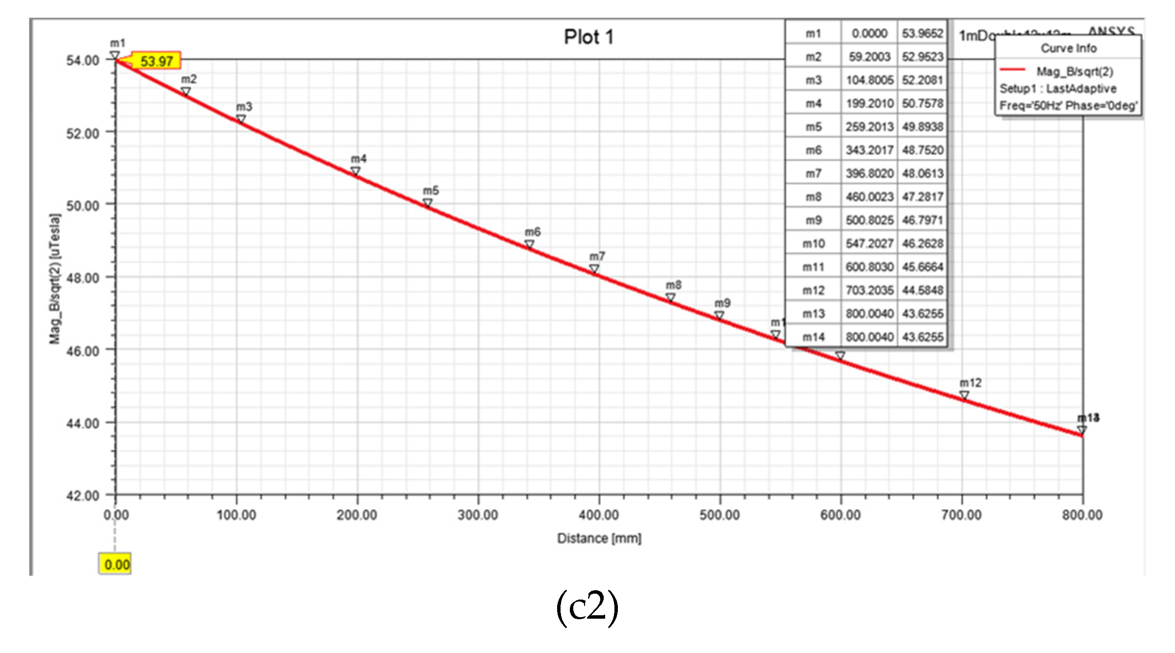
Simulation of the magnetic field distribution below a single-phase power transmission line, set on top of a living space, with a flat roof at a distance of 1 m from the power line. Field distribution without shielding (a1, a2), with single shielding layer (b1, b2) and double shielding layer (c1, c2).
Figure 15.
Simulation of the magnetic field distribution below a single-phase power transmission line, set on top of a living space, with a flat roof at a distance of 1 m from the power line. Field distribution without shielding (a1, a2), with single shielding layer (b1, b2) and double shielding layer (c1, c2).


Table 1.
Electric and magnetic field limits in different organizations.
| General Public | Occupational Groups | |
|---|---|---|
| ICNIRP (1998) 50 Hz | 5 kV/m, 100 μT | 10 kV/m, 500 μT |
| ICNIRP (1998) 60 Hz | 4.2 kV/m, 83 μT | 8.3 kV/m, 420 μT |
| IEEE (2002) 60 Hz | 5 kV/m, 904 μT | 20 kV/m, 2710 μT |
Publisher’s Note: MDPI stays neutral with regard to jurisdictional claims in published maps and institutional affiliations. |
© 2021 by the authors. Licensee MDPI, Basel, Switzerland. This article is an open access article distributed under the terms and conditions of the Creative Commons Attribution (CC BY) license (https://creativecommons.org/licenses/by/4.0/).
Share and Cite
MDPI and ACS Style
Damatopoulou, T.; Angelopoulos, S.; Christodoulou, C.; Gonos, I.; Hristoforou, E.; Kladas, A. On the Power Lines—Electromagnetic Shielding Using Magnetic Steel Laminates. Energies 2021, 14, 7215. https://doi.org/10.3390/en14217215
AMA Style
Damatopoulou T, Angelopoulos S, Christodoulou C, Gonos I, Hristoforou E, Kladas A. On the Power Lines—Electromagnetic Shielding Using Magnetic Steel Laminates. Energies. 2021; 14(21):7215. https://doi.org/10.3390/en14217215
Chicago/Turabian StyleDamatopoulou, Tatiana, Spyros Angelopoulos, Christos Christodoulou, Ioannis Gonos, Evangelos Hristoforou, and Antonios Kladas. 2021. "On the Power Lines—Electromagnetic Shielding Using Magnetic Steel Laminates" Energies 14, no. 21: 7215. https://doi.org/10.3390/en14217215
Note that from the first issue of 2016, this journal uses article numbers instead of page numbers. See further details here.