A New Model for Estimation of Energy Extraction from Bifacial Photovoltaic Modules

Abstract

The energy yield from bifacial solar photovoltaic (PV) systems can be enhanced by optimizing the tilt angle. Bifacial modules boost the energy yield by 4% to 15% depending on the module type and ground reflectivity with an average of 9%. The selection of tilt angle depends on several factors, including the geographical location, weather variation, etc. Compared to the variable tilt angle, a constant angle is preferred from the point of view of the cost of installation and the cost of maintenance. This paper proposes a new method for analysing bifacial modules. A simpler rear-side irradiance model is presented to estimate the energy yield of a bifacial solar photovoltaic module. The detailed analysis also explores the optimum tilt angle for the inclined south–north orientation to obtain the maximum possible yield from the module. Taking four regions into account, i.e., Kharagpur, Ahmedabad, Delhi, and Thiruvananthapuram, in the Indian climate, we studied several cases. The Kharagpur system showed a monthly rear irradiance gain of 13%, and the Delhi climate showed an average performance ratio of 19.5%. We studied the impact of albedo and GCR on the tilt angle. Finally, the estimated model was validated with the PVSyst version 6.7.6 as well as real field test measurements taken from the National Renewable Energy Laboratory (NREL) located in the USA.

1. Introduction

The increased interest in solar power becomes the key to the development of more efficient and different types of technology to harvest the sun rays [1]. To increase the energy capture, different methodologies are used. These include agronomic management [2] that promotes PV and agriculture, effective operational strategy of shading using bypass diodes [3], etc. Among all the technologies, another upcoming kind is bifacial PV. Bifacial PV modules can capture solar irradiance on both the front and rear surfaces. Unlike the monofacial PV with an opaque back cover, bifacial PV has a transparent back cover to allow the PV cells to receive backside irradiance.

In addition to lower LCOE, the bifacial PV modules have a longer lifetime for the glass-to-glass structure compared with traditional glass-back sheet module configurations, because the double glass module has lower cell temperature [4] and the rear glass can withstand an unfavorable environment. The rear back sheet is gradually degraded after being exposed to ultraviolet rays on the ground [5]. The development of photovoltaic energy has been very significant in recent years due to the cost reductions brought about by policy actions favouring the transition from a fossil fuels to a green society [6]. Those benefits will promote the development of bifacial PV modules among all kinds of PV technology, expanding its market from less than 5% in 2016 to 30% in 2027.

Dating back to the 1980s Guerrero-Lemus et al. performed a technical review of nearly 400 papers on bifacial PV modules published since 1979 [7]. The overall conclusion of that paper was to make bifacial technology more technically understandable and economically viable.

To understand the technology and the economics, it is required to understand its backside solar irradiance parameters and its electrical parameters [8]. Extensive investigations have been conducted on the performance of monofacial PV and its mathematical modelling. Though the advantages of bifacial modules have been shown in many research articles, a proper mathematical model for the estimation of solar irradiance is somewhat lacking [9].

Conceptually, total irradiance on the rear side of the bifacial module results from the addition of:

• Direct irradiance.
• Ground reflected irradiance, which depends on the albedo .
• Sky diffuse irradiance.

In previous papers [10,11,12,13,14,15,16], ray tracing, view factor, and empirical models were discussed to estimate backside irradiance. However, these methods have certain drawbacks. A comparison of the view factor and the ray-tracing model is established in [17], where measurements and simulations for front and rear side irradiance values for one sample day showed consistency at the cell and module level. Several other researchers investigated the performance of a single bifacial PV module [18].

The ray-tracing approach simulates the multipath reflection and absorption of an individual ray entering a scene while the view factor approach, assumes isotropic scattering of reflected rays and, thus, permits the calculation of irradiance by integration. The empirical models represent the relationship between measured quantities [19]. However, in the ray-tracing approach, the execution time is overly high. The view factor approach assumes an infinite number of rows and a Lambertian isotropic sky. The empirical model, developed by Castillo-Aguilella et al. from prism solar technologies, allows yearly gain calculations for a single module [20]. Although the climate is not considered, the model is suggested for latitudes between ${21}^{\circ }$ to ${51}^{\circ }$ from the equator.

In [21], a mathematical model is discussed considering shading and reflection. It has been suggested that, for significant energy improvement, a simple arrangement of a white painted surface is made to generate higher albedo. A combination of a white painted wall and ground surfaces, if well oriented, can result in a more than 60% increase in radiation.

In [22] the view factor approach was used for the front irradiance and ray tracing for the rear side irradiance. The paper suggested that the view factor concept allows for an accurate prediction of the energy yield for the bifacial fixed-tilt system, whereas the ray tracing is accurate for the bifacial horizontal single-axis tracking (HSAT) system. In [23], performance models for bifacial modules are discussed. In some works of literature, the view factor approach was adopted for modelling [24].

Bifacial PV modules can be installed in the conventional south-facing orientation or even east–west ($E-W$), keeping the modules vertical to the Earth’s plane [25]. Vertically mounted bifacial modules were studied thoroughly in [26]. Vertically mounted panels are advantageous as the energy yield is higher; in addition, dust accumulation is lower in the case of a vertical mount.

This work’s main objectives are (1) to measure the performance of bifacial PV (2) to develop and validate the model of backside irradiance. In this paper, for the estimation of rear side irradiance, a more accurate, simpler model is proposed. Here, the concept of solar geometry [27] is used for estimation of the rear side irradiance bifacial PV module. Earlier, in many kinds of literature, the same concept has been used for front-side energy estimation. By modifying the geometrical features of the spherical coordinates, the necessary parameters for rear side modelling are ensured.

Solar geometry is a spherical coordinate system that involves the position of the Sun with the Earth. Using this concept, the irradiance of the rear side bifacial module is estimated. The optimum tilt angle for bifacial south–north panels has also been explored. Taking four different regions in India as examples, we studied four orientations. The results are compared with the PVSyst version 6.7.6 [28] while keeping all necessary input parameters the same.

The model presented here can potentially explore the effects of detailed features in the module and array design, such as spacing between modules, which cannot be easily addressed in the view factor model. The mathematical equation for the front side of the PV is well established in the literature; however, there are no such mathematical equations available for the rear side. Using the proposed model, the same can be easily derived for rear side PV. In addition to this, the view factor approach assumes an infinite number of rows and a Lambertian isotropic sky; however, in the presented work, no such assumptions are made. In the following sections, the rear side irradiance model used by PVSyst is briefly discussed to obtain more insight into the usefulness of the new model presented here.

2. Rear Side Irradiance Model Used by PVSyst

The rear side irradiance modelling is divided into three categories:

• Ray tracing models.
• View factor models.
• Empirical models.

PVSyst uses the view factor model for the calculation of rear side irradiance. It represents the portion of the radiation that leaves surface A and strikes another surface B. It is taken from the concept of thermal radiation heat transfer and applied to model the rear side irradiance of the bifacial modules. A fundamental hypothesis of PVSyst is that the light re-emitted by a point on the ground has an isotropic distribution. This means that the light is re-emitted with the same intensity, whatever the direction of space. There is no other reflection. This is Lambertian distribution, i.e., each ray is multiplied by the cosine of the incidence angle.

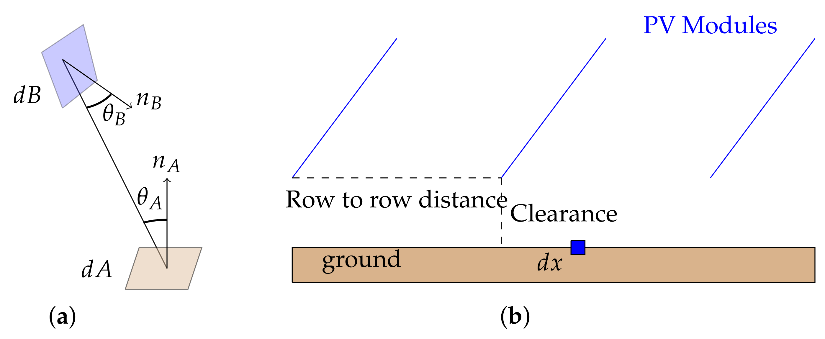
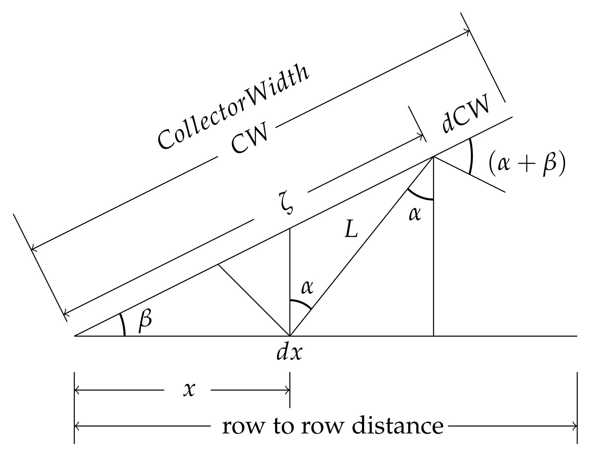
The irradiance from a ground segment reaching the rear-side of a solar module can be estimated by considering an infinitely long row of solar modules, as shown in cross-section Figure 1. The procedure described below to calculate view factor values, for this particular case is adapted from [29]. The view factor $d{F}_{dx-dCW}$ between the differential segment of ground $dx$ and the differential segment of collector width $dCW$ is:

$$d{F}_{dx-dCW}=\frac{1}{2}cos\alpha d\alpha$$

(1)

where $d{F}_{dx-dCW}$ is in terms of the distance x wrt the differential ground segment and distance from the origin of collector wrt the differential segment of the collector ($\zeta$) and the tilt of the modules ($\beta$) as shown in Figure 2.

$\alpha$ is the cosine of the angle between the normal of the ground surface and the vector connecting the ground and module segments under analysis. d$\alpha$ is the angle subtended by the projection of $dCW$ normal to L, that is:

$$d\alpha =\frac{d\zeta cos(\beta +\alpha )}{L}=\frac{d\zeta }{L}\frac{xsin\beta }{L}$$

(2)

$$cos\alpha =\frac{\zeta (sin\beta )}{L}$$

(3)

Then,

$$\begin{array}{cc}\hfill d{F}_{dx-dCW}& =\frac{1}{2}cos\alpha d\alpha \hfill \\ \hfill & =\frac{1}{2L^3}\zeta xsi{n}^2\beta d\zeta \hfill \\ \hfill & =\frac{\zeta xsi{n}^2\beta }{2{(x^2+{\zeta }^2-2\zeta xcos\beta )}^{3/2}}d\zeta .\hfill \end{array}$$

(4)

For calculating the irradiance in the rear side of the solar module, view factors are calculated between the ground and the sky, the rear side of the module, and each ground segment. All these calculations are done in terms of irradiance. The involved energy should be renormalized by the concerned area, i.e.,

• the total energy on the ground is the irradiance multiplied by the total ground area concerned by the installation; and
• the total energy on the rear side is the irradiance multiplied by the collector’s area.

Therefore, the energy ratio computed by the view factor integral should be multiplied by the area ratio:

Irradiance (rear) = Irradiance (ground) × View factor × (ground area/collectors area).

The view factor model assumes that all the reflecting surfaces are Lambertian, i.e., the irradiance is scattered isotropically. The structure-reflected irradiance component depends on the position within the array; modules near the middle of a row should see more reflected irradiance than the modules at the ends of a row. Similarly, modules near the ends of a row should see higher sky diffuse irradiance than a module in the row’s middle, because less of the sky is blocked from view by nearby rows. This affects the ground reflected component of the backside irradiance.

3. Modelling Approach

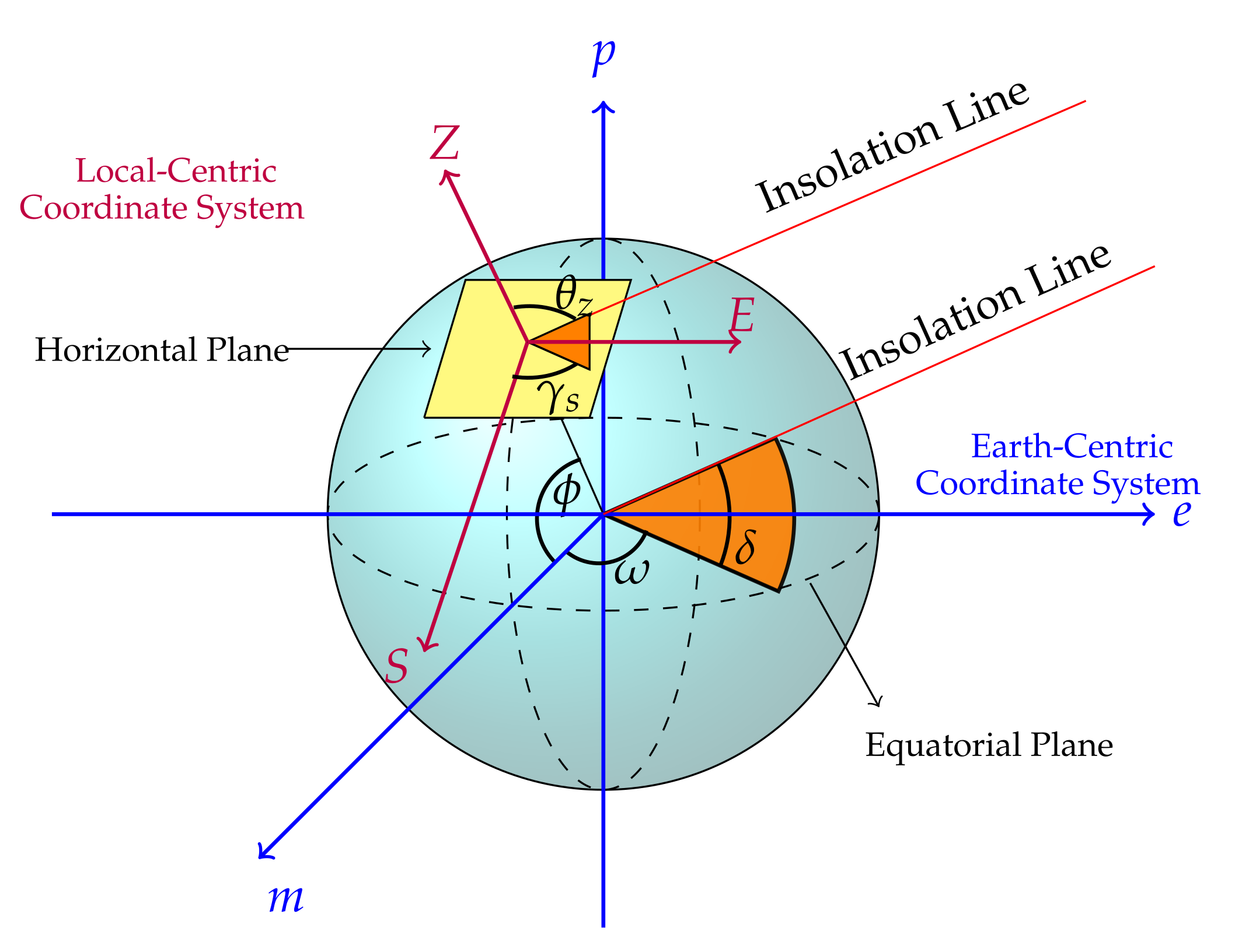
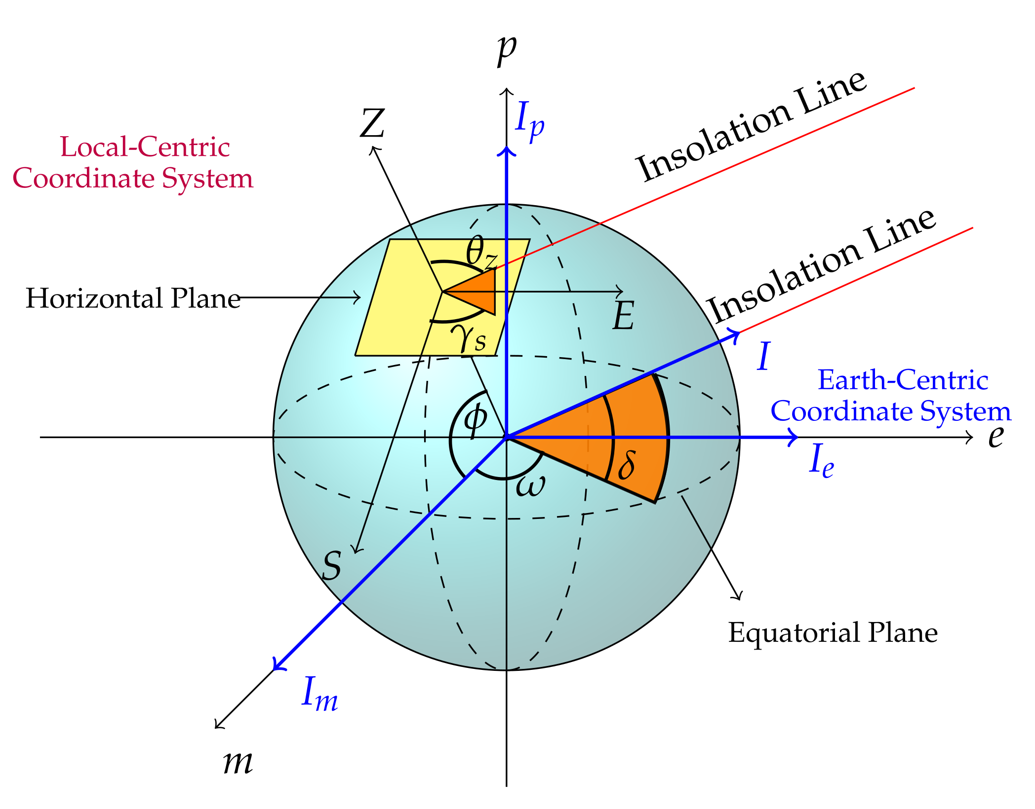
Solar geometry is used to estimate the irradiance of the bifacial panel front and rear sides at any given location on the surface of Earth. It is nothing but the spherical coordinate system that involves the position of the Sun with the Earth. Figure 3 shows the coordinates of a $3D$ system, considering Earth at the centre.

A quarter portion of the Earth has been cut and made the $3D$ coordinate system, as shown in Figure 3. The Centre of the Earth and that of the distant Sun are connected by a line called the insolation line. An equatorial plane is considered, which cuts across the globe at the equator. This acts as a reference plane, and the angle of declination ($\delta$) is measured to that.

The declination and hour angle are shown for the meridional plane and the insolation line [30]. Three axes of the Earth-centric coordinate system are the polar axis p, meridional axis m, and eastern meridian axis e. The eastern meridian axis is orthogonal to the above two axes, as shown in Figure 3. Hence, the equatorial plane along with the three coordinate axes is called the Earth-centric coordinate system.

A point of interest on the Earth’s surface is the location where the irradiance is calculated. The line passing through the point of interest and the centre of Earth intersecting a specific latitude and longitude will become the origin of the local coordinate system. A tangential plane is placed on that local point called a horizon plane, which is orthogonal to the line joining latitude point and the centre of Earth.

The line that is normal to the Horizon plane going straight up vertically is the zenith axis Z, the second one that goes tangential to the meridional plane going down south along the Horizon plane will be denoted as S, representing south. The third coordinate axis is shown east as E to distinguish between the lowercase e, which is used for the Earth-centric coordinate system.

The E axis of the local coordinate and e axis of the Earth coordinate system are parallel with each other, pointing in the same direction. Hence, the zenith, south, and east axis, along with the reference horizon plane, form the local-centric coordinate system. The insolation line makes an angle to the vertical axis or the zenith axis, called the zenith angle ${\theta }_z$ [30].

There is one more term called the azimuth angle ${\gamma }_s$. This is an angle on a horizontal plane between the line due south and the projection of the insolation line onto the horizon plane. $\varphi$ is called the latitude angle, as shown in Figure 3. This is the vertical angle between the line joining that point of location to the centre of Earth and its projection on the equatorial plane.

3.1. Solar Irradiance on the Horizontal Plane

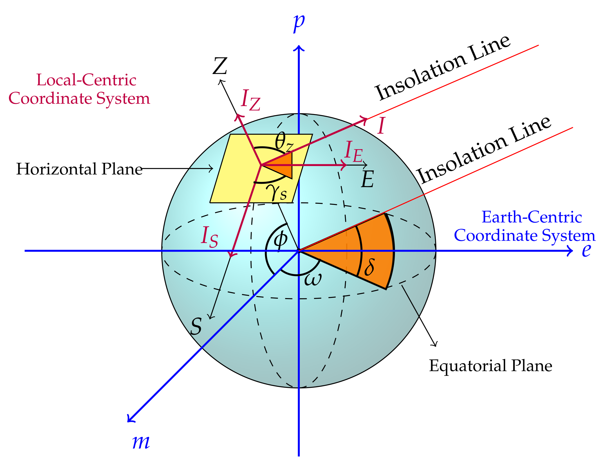
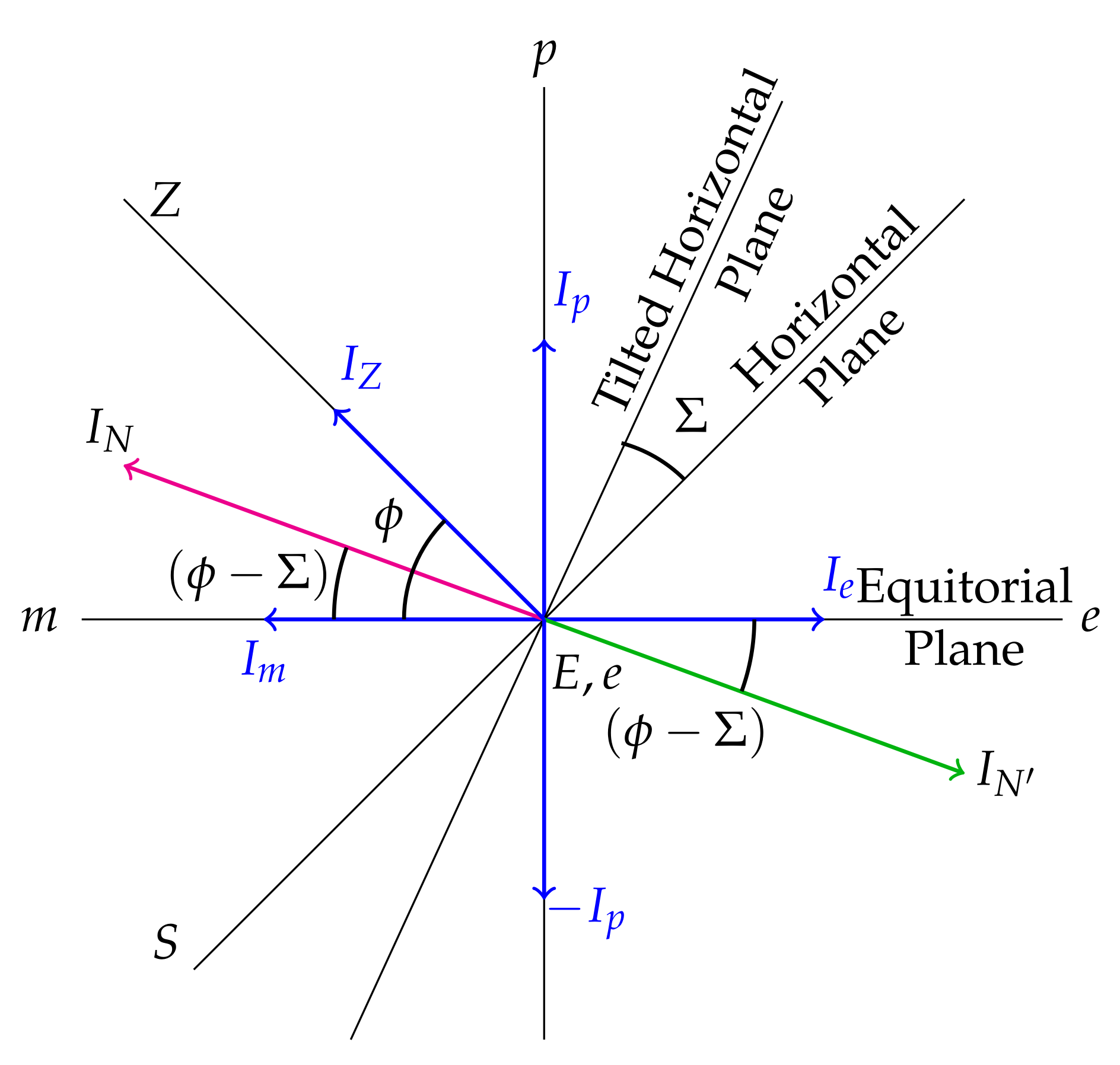
A horizontal plane is kept tangential to the locality point as shown in Figure 4. The amount of normal incidence of solar insolation falling on the surface is calculated by using a vector I on the insolation line as shown. This represents the irradiance from the Sun falling on it. This insolation vector can be resolved into orthogonal components along all three axes of the local coordinate system, i.e., $I_S$, $I_E$, and $I_Z$.

$$\begin{array}{c}\hfill I=I_S+I_E+I_Z\end{array}$$

(5)

where

$$\begin{array}{cc}\hfill I_S& =Isin{\theta }_{z}cos{\gamma }_s,\hfill \end{array}$$

(6)

$$\begin{array}{cc}\hfill I_E& =Isin{\theta }_{z}sin{\gamma }_s,\hfill \end{array}$$

(7)

$$\begin{array}{cc}\hfill I_Z& =Icos{\theta }_z.\hfill \end{array}$$

(8)

$I_S$ is the component along the south axis, $I_E$ along the east axis, and $I_Z$ along the zenith axis. $I_Z$ is vertical normal to the horizon plane. Hence, it will give effective irradiance at the place on the horizontal flat plate collector. $I_S$ and $I_E$ are along with the horizontal flat plate, and thus they do not contribute to any effective irradiance. Therefore, it is essential to find the value of $I_Z$.

${\theta }_z$ is the zenith angle, and it cannot be directly calculated; therefore, we attempted to estimate it from the known parameters, like the latitude angle, known from the location of the place, hour angle, and declination angle, which depends on the time and number of the day.

Again, a vector I is considered along the insolation line of the Earth-centric coordinate system, as shown in Figure 5. Similarly, vector I can be resolved into three orthogonal components, i.e., $I_p$ along the polar axis, $I_m$ along the meridional axis, and $I_e$ along the east axis.

$$\begin{array}{cc}\hfill I& =I_e+I_m+I_p\hfill \end{array}$$

(9)

where

$$\begin{array}{cc}\hfill I_e& =Icos\delta sin\omega ,\hfill \end{array}$$

(10)

$$\begin{array}{cc}\hfill I_m& =Icos\delta cos\omega ,\hfill \end{array}$$

(11)

$$\begin{array}{cc}\hfill I_p& =Isin\delta .\hfill \end{array}$$

(12)

The above-resolved vectors are in terms of $\delta$ and $\omega$. Hence, these are easily determinable. Therefore, for calculating local-centric coordinate system components, a relation between an Earth-centric and local-centric coordinate system need to be established. However, the two systems have different origins. Thus, one assumption is made; the radius of Earth is minimal as compared to the distance between Earth and Sun. Hence, insolation lines that are parallel to two systems can be merged. Merged $2D$ vector representation, as shown in Figure 6. $I_Z$ can be resolved into $I_m$, and $I_p$;

$$\begin{array}{cc}\hfill I_Z& =I_{m}cos\varphi +I_{p}sin\varphi \hfill \end{array}$$

(13)

Substituting the value of $I_m$ and $I_p$ in (13), The modified value for $I_Z$ will be

$$\begin{array}{c}\hfill I_Z=I(cos\delta cos\omega cos\varphi +sin\delta sin\varphi ),\end{array}$$

(14)

where I is the extra terrestrial insolation in kW/m${}^2$,

$$\begin{array}{c}\hfill I=I_{sc}\left(1+0.035cos\frac{360n}{365}\right),\end{array}$$

(15)

$I_{sc}$ is a solar constant, i.e., 1.37 kW/m${}^2$. At noon, $\omega$ is zero. The Hour angle to the east of noon is considered positive, and that of to the west is negative. Sunrise occurs toward the east of the meridional axis; therefore, at sunrise, the hour angle is positive, and, at sunset, it is negative.

3.2. Solar Irradiance on a Tilted Plane

A plane is considered that is inclined from the horizontal surface at an angle $\Sigma$, as shown in Figure 7. At the front and rear sides of the tilted plane, two vector axes N and $N^{\prime }$ are taken, perpendicular to the tilted surface at the front and rear sides, respectively, and irradiance along those vectors are named $I_N$ and $I_{N^{\prime }}$. These two vectors are different from each other.

Then, the vectors $I_N$ and $I_{N^{\prime }}$ will be

$$\begin{array}{c}\hfill I_N=I_{m}cos(\varphi -\Sigma )+I_{p}sin(\varphi -\Sigma )\end{array}$$

(16)

$$\begin{array}{c}\hfill I_{N^{\prime }}=I_{m}cos(\varphi -\Sigma )-I_{p}sin(\varphi -\Sigma )\end{array}$$

(17)

substituting the values of $I_m$ and $I_p$ in (16) and (17),

$$\begin{array}{c}\hfill I_N=I(cos\delta cos\omega cos(\varphi -\Sigma )+sin\delta sin(\varphi -\Sigma ))\end{array}$$

(18)

$$\begin{array}{c}\hfill I_{N^{\prime }}=I(cos\delta sin\omega cos(\varphi -\Sigma )-sin\delta sin(\varphi -\Sigma ))\end{array}$$

(19)

3.3. Summary of the Model Equations

The front and rear side direct irradiances of the bifacial PV module calculated using the spherical solar coordinate geometry. Two orientations are considered here for the study. Hence, two folds of equations can be summarized as shown below;

3.3.1. South–North Orientation

Solar panels installed at locations on the south side of the equator should face north, and those installed at locations on the north side of the equator should face south. Here, south–north orientation is taken as an example. The estimated direct irradiance will be,

$$\begin{array}{cc}\hfill I_N& =I_{B}cos\theta \hfill \end{array}$$

(20)

$$\begin{array}{cc}\hfill I_{N^{\prime }}& =\frac{I_{B}cos\theta }{2}\left((cos\delta cos\omega cos(\varphi -\Sigma )-sin\delta sin(\varphi -\Sigma \left)\right)\right)\hfill \end{array}$$

(21)

(20) and (21) represent direct irradiance for front and rear side respectively.

Global irradiance can be the combination of direct, reflected, and sky diffused irradiance for the front as well as the rear side.

$$\begin{array}{cc}\hfill I_{global,front}& =I_N+I_{RC}+I_{DC},\hfill \end{array}$$

(22)

$$\begin{array}{cc}\hfill I_{global,rear}& =I_{N^{\prime }}+I_{RC}+I_{DC}.\hfill \end{array}$$

(23)

3.3.2. Vertical East–West Orientation

Generally vertical installation facing the east side has better performance as compared to the south–north orientation. Direct irradiance for the front as well as rear side of a vertically installed PV module will be

$$\begin{array}{c}\hfill I_M=I_{B}cos\theta (1-Y),\end{array}$$

(24)

$$\begin{array}{c}\hfill I_{M^{\prime }}=I_{B}cos\theta (1-X).\end{array}$$

(25)

where

$$\begin{array}{c}\hfill Y=cos\delta sin\omega sin\varphi +sin\delta cos\varphi ,\end{array}$$

(26)

$$\begin{array}{c}\hfill X=cos\delta cos\omega sin\varphi -sin\delta cos\varphi .\end{array}$$

(27)

The global irradiance will be,

$$\begin{array}{cc}\hfill I_{global,front}& =I_M+I_{RC}+I_{DC}\hfill \end{array}$$

(28)

$$\begin{array}{cc}\hfill I_{global,rear}& =I_{M^{\prime }}+I_{RC}+I_{DC}\hfill \end{array}$$

(29)

from [30], the values of $I_{RC}$, $I_{DC}$, and C are

$$\begin{array}{cc}\hfill I_{RC}& =\rho (I_{BH}+C{I}_B)\left(\frac{1-cos\Sigma }{2}\right)\hfill \end{array}$$

(30)

$$\begin{array}{cc}\hfill I_{DC}& =C{I}_B\left(\frac{1+cos\Sigma }{2}\right)\hfill \end{array}$$

(31)

$$\begin{array}{cc}\hfill C& =0.095+0.04sin\left(\frac{360(n-100)}{365}\right)\hfill \end{array}$$

(32)

From [31], it was shown that the albedo coefficient significantly affected the efficiency and resulting power output. The albedo coefficient of snow, white sand, and green grass led to higher than expected power output. In the case of snow, it was increased by 7.5%, and in the case of white sand, it was increased by 4%. An ideal spectral albedo for the maximum power output and minimum heat impact was derived in [31]. Hence, for verification purpose, here, the albedo coefficient is taken as 0.5.

4. Validation and Results

The estimated model was applied to evaluate the irradiance for both the front and rear side of the bifacial module for four different regions of the Indian climate at their optimum tilt angles facing south and at 90${}^{\circ }$ facing east. Before going to the validation, optimization of the tilt angle for each location mentioned was performed.

4.1. Tilt Angle Optimization

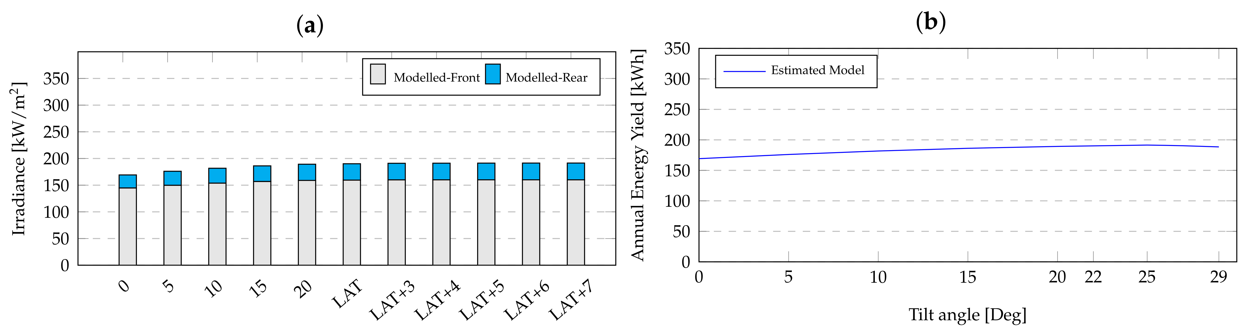
To have the maximum energy yield at any particular location, optimization of the tilt angle is necessary. The optimum tilt angle was found using the estimated model by varying the tilt angle from 0${}^{\circ }$ to 7${}^{\circ }$ more than the latitude of that location, as shown in Figure 8. The irradiance of both sides was noted down and analysed, which gave higher irradiance in total. That tilt angle corresponding to higher irradiance was the optimum tilt angle. Hence, we can see, from

Table 1. The optimum tilt angles for different locations.

Location	Latitude	Optimum Tilt Angle
Kharagpur	22.34° N, 87.23° E	24°
Ahmedabad	23.02° N, 72.57° E	25°
Delhi	28.70° N, 77.10° E	31°
Thiruvananthapuram	8.52° N, 76.93° E	10°

, the optimum tilt angle, by the model, was on an average $2{}^{\circ }$ more than the latitude.

The tilt angle optimization is performed by creating a database that stores the average hourly irradiance over a year. To do this, the first monthly average data is created. Considering the irradiance for a particular tilt angle at a definite time (on an hourly basis) of the day, the data is averaged and the hourly variation of irradiance for every month is, thus, found. Following this, the hourly variation of irradiance for a year is found by averaging the monthly data. Thus, the energy capture can easily be found on a particular year for a particular tilt angle at a particular location.

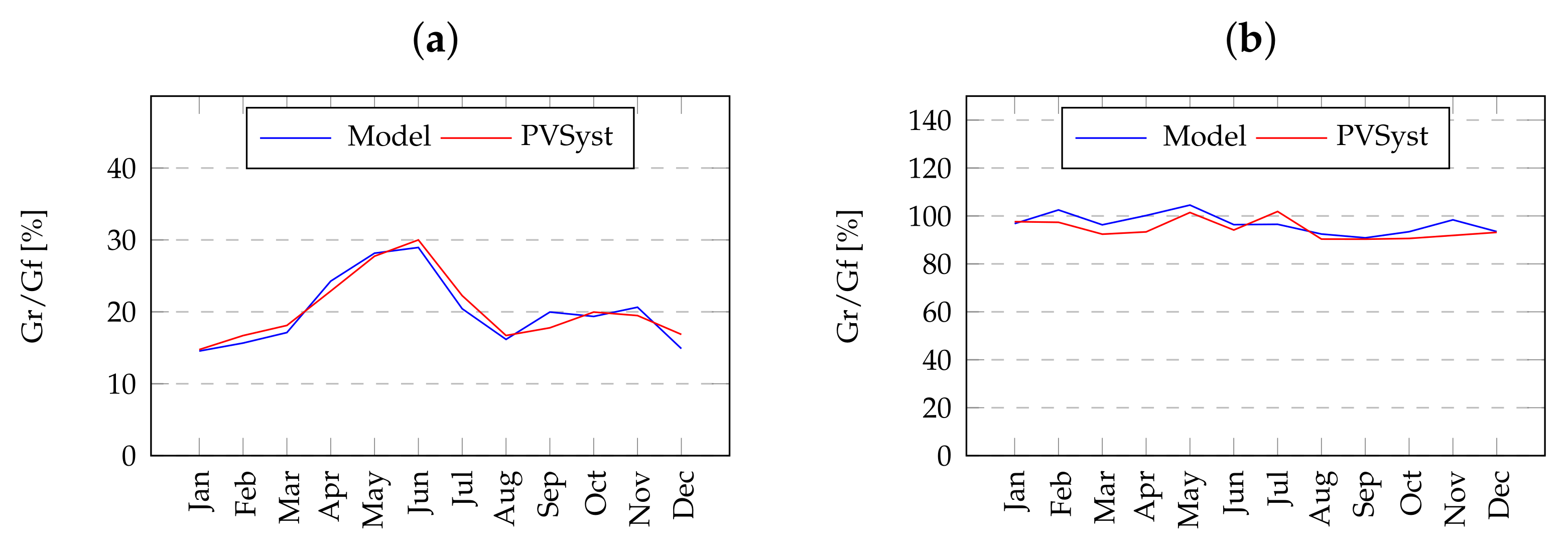
Therefore, we concluded that the optimum tilt angle for the Kharagpur location was 24${}^{\circ }$. The similar studies we performed for the other three locations and the optimum tilt angles for the bifacial PV are listed in Table 1.

4.2. Investigation of the Difference between Bifacial and Monofacial PV at Different Tilt Angles

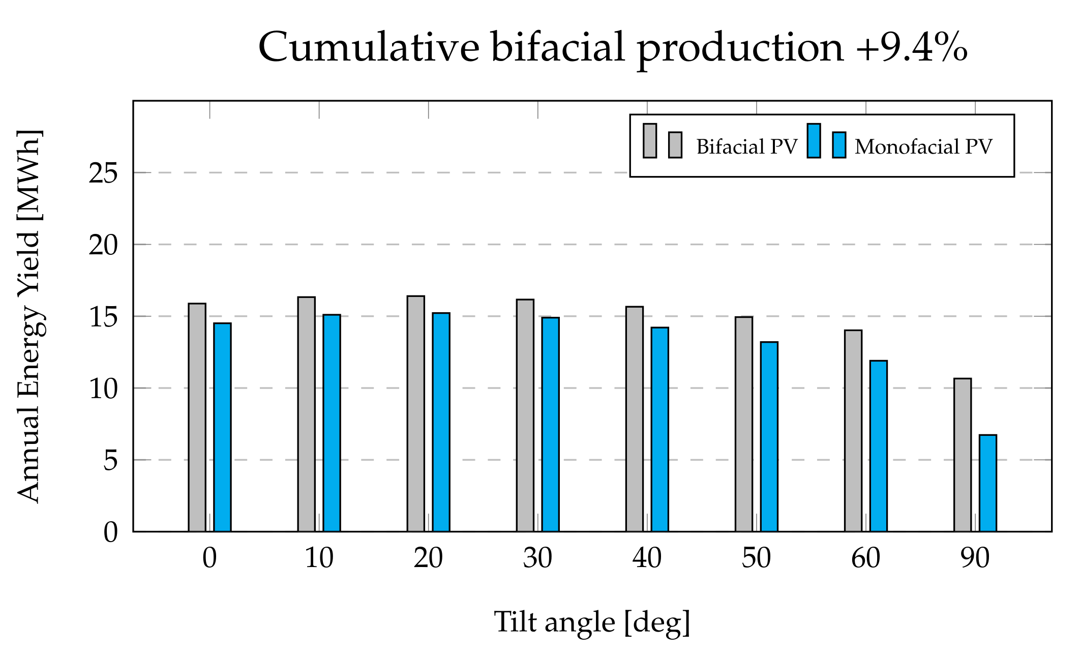
A comparison study was conducted using PVSyst to compare the annual energy yield (array output) between bifacial and monofacial PV at different tilt angles. For this study, the array size for monofacial and bifacial PV was taken as 10 kWp. The tilt angle from 0${}^{\circ }$ to 90${}^{\circ }$ was varied keeping other simulation parameters constant. For investigation, the PVSyst simulation parameters taken are listed in

Table 2. Simulation parameters.

Parameters	Bifacial PV	Monofacial PV
No. of modules	24	24
Module area	54 m${}^2$	48 m${}^2$
No. of inverters	3	3
Nominal PV power	10 kWp	10 kWp
Maximum PV power	9.5 kWDC	7.4 kWDC
Nominal AC power	9 kWAC	9 kWAC
Pnom Ratio	1.11	1.11

.

For comparison of bifacial and monofacial PV in the PVSyst software, the GCR was set at 0.66, the pitch was 1.5 m, and the panel width was 1 m. For bifacial PV, the albedo was considered at 0.55. For bifacial modules, the height above ground was taken as 1 m. From Figure 9, we observed that, at a particular tilt angle, the annual energy yield of bifacial PV was 9.4% higher than that of monofacial PV.

4.3. Impact of Albedo and GCR (Ground Clearance Ratio)

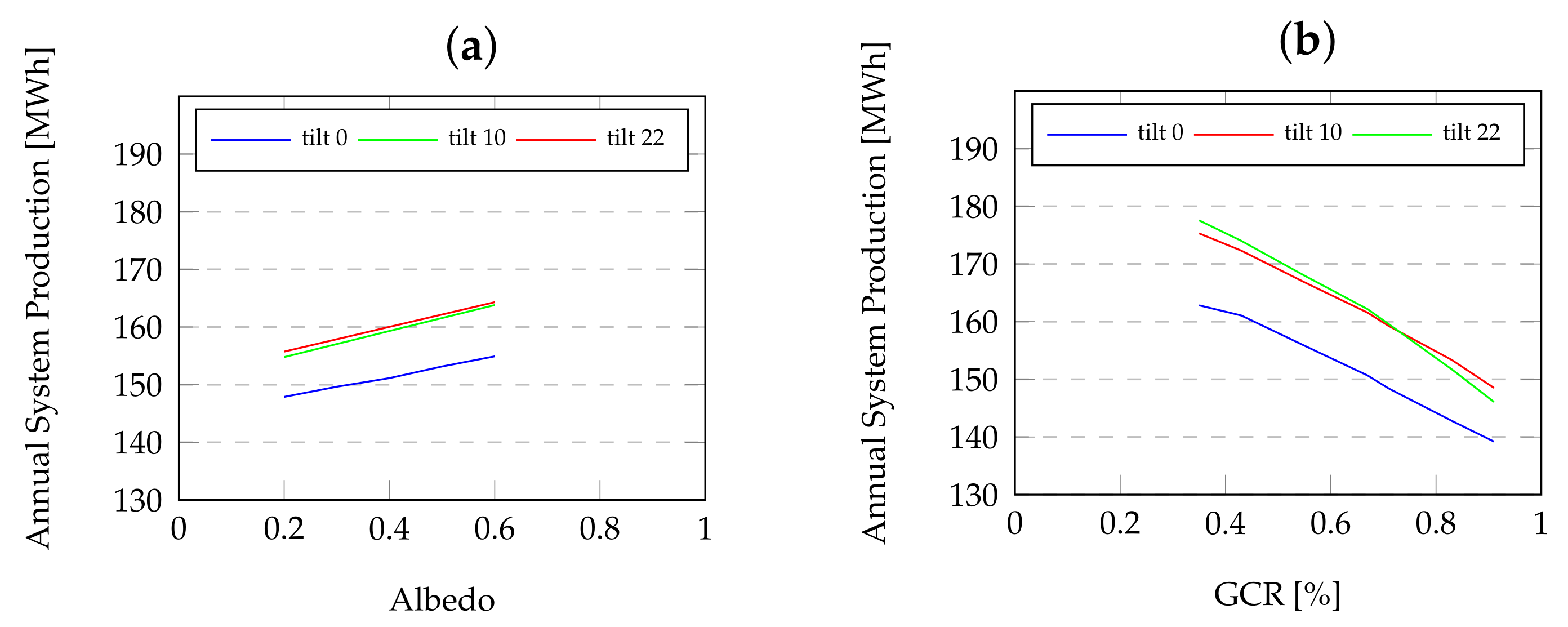
Keeping the albedo at 0.5, for the location Kharagpur ($22.34$${}^{\circ }$ N, $87.23$${}^{\circ }$ E), the ground clearance ratio (GCR) varied from 0 to 1. From the figure, with changing GCR, the optimum tilt angle will not change; however, the annual energy production will increase with decreasing GCR. A similar study was performed by keeping the GCR constant and changing the albedo value from 0 to 1. By Figure 10, we inferred that, with a higher albedo value, the annual production will increase; however, this will not affect the optimum tilt angle. Here, for investigation, a 10 kW bifacial system was used. Thus, the annual system production was MWh per 10 kW.

4.4. Comparison with PVSyst V6.7.6

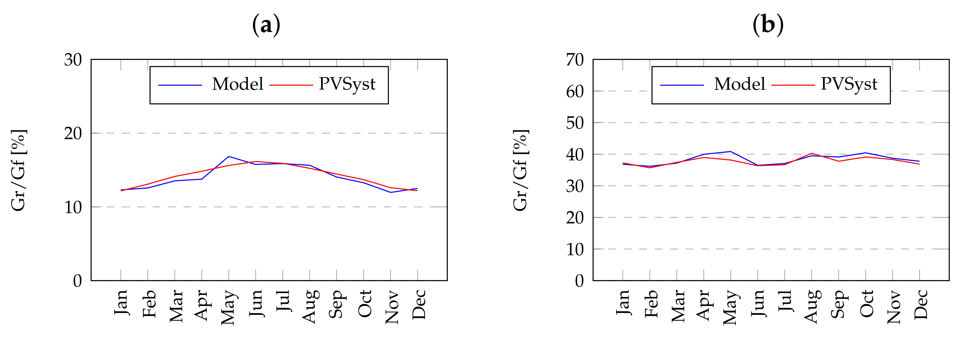
The bifacial PV module front and rear energy productions were analysed from Jan to Dec of the year 2019 and compared with the PVSyst simulation monthly irradiance. Four different orientations are discussed, i.e., the front and rear side for the south-facing tilted module and the vertical mount facing east. Estimation using the proposed model had good agreement with the PVSyst results. For the simulation in PVSyst, the bifacial array size was taken as 10 kW. To avoid inverter clipping in the PVSyst simulation, the DC/AC ratio was taken as 1.11. For the location Kharagpur, the percentage gain (Gr/Gf) for SN orientation was 19.5% and, for EW vertical orientation, was 95%.

Figure 11, Figure 12, Figure 13 and Figure 14 show the comparison between estimated model irradiance for the front and rear side of the bifacial panel and PVSyst simulation taking four regions into consideration, i.e., Kharagpur, Delhi, Ahmedabad, and Thiruvananthapuram. The site albedo is not known accurately; however, based on tables of albedo from [29], short grass typically has values of 0.15–0.5. Here, a typical value of 0.5 was assumed.

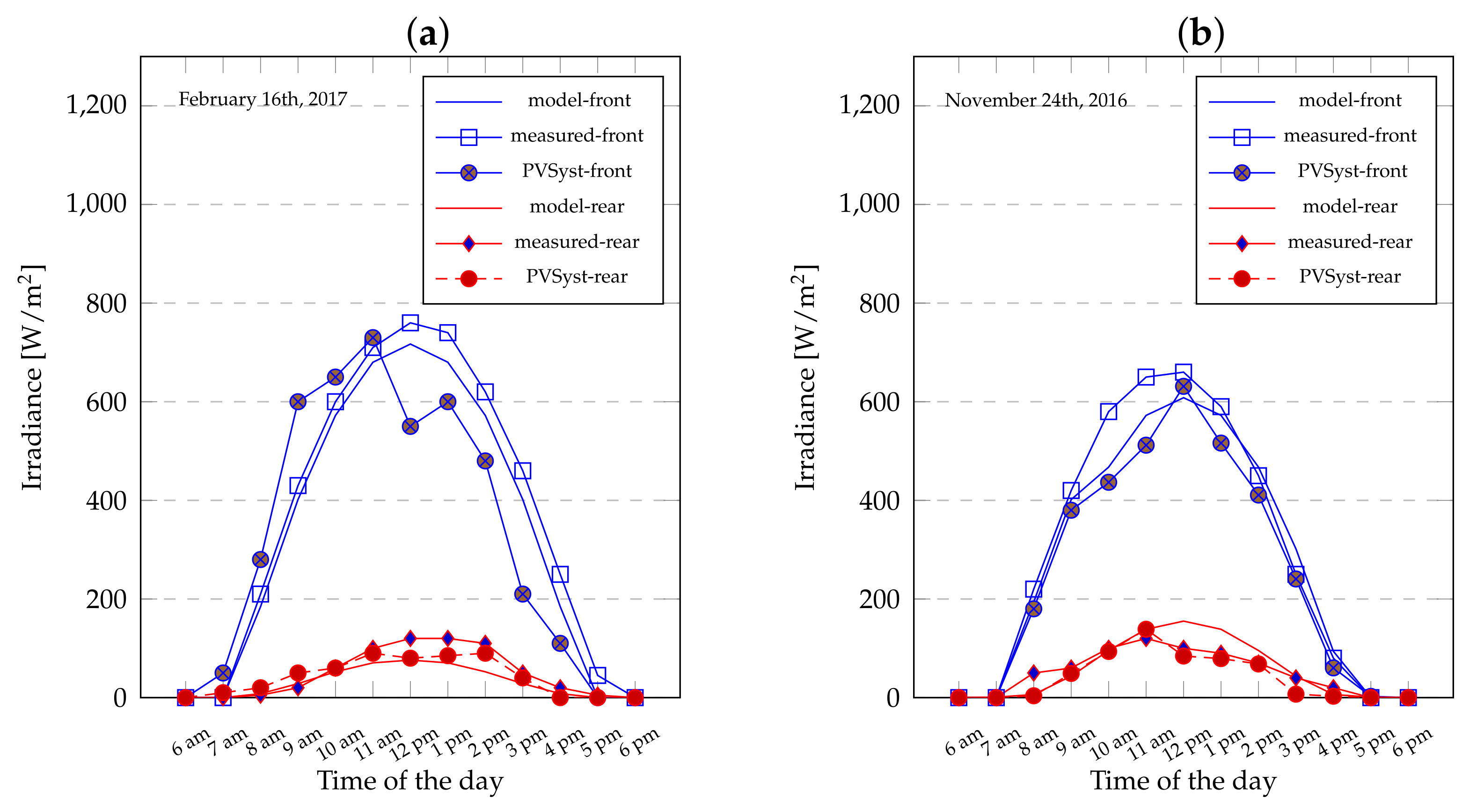
4.5. Validation with Real Field Measured Values

For proper validation of the proposed estimation, the measured field irradiance was taken from NREL, USA [32]. The installed bifacial PV plant was at 15${}^{\circ }$ tilt facing south with an albedo coefficient of 0.55. The date of measurement was taken as 16 February 2017 and 24 November 2016. NREL is situated at latitude 39.741${}^{\circ }$ N and longitude 105.1725${}^{\circ }$ W. The azimuthal is 165${}^{\circ }$, with a normalized row gap of 0.56, GCR (Ground Clearance Ratio) of 0.65, and normalized clearance height of 0.52. The source irradiance used in PVSyst and the model simulation for the NREL location is listed in

Table 3. Source irradiance data used in PVSyst and the model simulation (Feb 2017).

Time of the Day	Global Horizontal Irr. [W/m${}^2$]	Diffuse Horizontal Irr. [W/m${}^2$]
6 am	0	0
7 am	0	0
8 am	250.2	41.9
9 am	588.8	91.8
10 am	642.8	137.3
11 am	729.2	274.99
12 pm	566.9	251.09
1 pm	593.89	187.00
2 pm	480.7	140.3
3 pm	295.4	168.4
4 pm	264.7	124.4
5 pm	124.8	67.6
6 pm	3.09	3.10

.

We inferred from Figure 15 that the proposed model had energy extraction with higher accuracy compared with that of PVSyst, both for the front and rear sides of the bifacial PV module. A dip in irradiance at 12 pm in the PVSyst simulation was possibly due to an artefact in the satellite output.

As the site was held constant for all simulations, the site meteorological and albedo inputs into the PVSyst program were the same for the configurations. In addition to that, the GCR, normalized clearance height, and normalized row gap were held constant for the simulations.

5. Conclusions

The bifacial solar PV system is an emerging area of research. The use of bifacial modules can increase the energy capture, and hence a higher amount of solar power can be harnessed from the same area compared to standard monofacial systems. From the study, we proved that bifacial modules boosted the energy yield by 4% to 15% depending on the module type and ground reflectivity with an average of 9%. This paper dealt with the estimation of the total irradiance (front and rear sides) from a bifacial PV system that was installed in an inclined position with front panels facing south and in a vertical position with front panels facing east.

The purpose of the vertical mount is to ensure a higher energy yield during the late afternoon hours. The Kharagpur System showed a performance ratio of 13% for the SN orientation and 80% for the EW vertical orientation. The proposed model showed a higher accurate energy extraction from the bifacial PV. A comparison of the model was made using PVSyst version 6.7.6. Furthermore, after analysing the optimum tilt angle for the locations mentioned, we concluded that, for bifacial modules, the optimum tilt angle was $2{}^{\circ }$ (on average) more than the latitude of that particular location. The estimated annual energy yield was also compared with that of PVSyst, and the former had higher annual energy generation.

For further validation of the proposed estimation, we compared with field test measurements taken from NREL, USA. We concluded that the field measurements showed a good agreement with the proposed estimation. Hence, the model can be used to optimize the tilt angle, and also it can help in estimating the energy yield before an installation can be made. The proposed analysis and estimation method will help to accurately predict the energy yield from bifacial systems, thus, further promoting this emerging technology.

References

- Piasecka, I.; Bałdowska-Witos, P.; Piotrowska, K.; Tomporowski, A. Eco-energetical life cycle assessment of materials and components of photovoltaic power plant. Energies 2020, 13, 1385. [Google Scholar] [CrossRef] [Green Version]
- Zainol Abidin, M.A.; Mahyuddin, M.N.; Mohd Zainuri, M.A.A. Solar Photovoltaic Architecture and Agronomic Management in Agrivoltaic System: A Review. Sustainability 2021, 13, 7846. [Google Scholar] [CrossRef]
- Vieira, R.G.; de Araújo, F.M.; Dhimish, M.; Guerra, M.I. A comprehensive review on bypass diode application on photovoltaic modules. Energies 2020, 13, 2472. [Google Scholar] [CrossRef]
- Lamers, M.; Özkalay, E.; Gali, R.; Janssen, G.; Weeber, A.; Romijn, I.; Van Aken, B. Temperature effects of bifacial modules: Hotter or cooler? Sol. Energy Mater. Sol. Cells 2018, 185, 192–197. [Google Scholar] [CrossRef]
- Carolus, J.; Tsanakas, J.A.; van der Heide, A.; Voroshazi, E.; De Ceuninck, W.; Daenen, M. Physics of potential-induced degradation in bifacial p-PERC solar cells. Sol. Energy Mater. Sol. Cells 2019, 200, 109950. [Google Scholar] [CrossRef] [Green Version]
- D’Adamo, I.; Gastaldi, M.; Morone, P. The post COVID-19 green recovery in practice: Assessing the profitability of a policy proposal on residential photovoltaic plants. Energy Policy 2020, 147, 111910. [Google Scholar] [CrossRef] [PubMed]
- Guerrero-Lemus, R.; Vega, R.; Kim, T.; Kimm, A.; Shephard, L. Bifacial solar photovoltaics—A technology review. Renew. Sustain. Energy Rev. 2016, 60, 1533–1549. [Google Scholar] [CrossRef]
- Qais, M.H.; Hasanien, H.M.; Alghuwainem, S. Parameters extraction of three-diode photovoltaic model using computation and Harris Hawks optimization. Energy 2020, 195, 117040. [Google Scholar] [CrossRef]
- Gu, W.; Ma, T.; Ahmed, S.; Zhang, Y.; Peng, J. A comprehensive review and outlook of bifacial photovoltaic (bPV) technology. Energy Convers. Manag. 2020, 223, 113283. [Google Scholar] [CrossRef]
- Robinson, D.; Stone, A. Irradiation modelling made simple: The cumulative sky approach and its applications. In Proceedings of the PLEA Conference, Eindhoven, The Netherlands, 19–21 September 2004; pp. 19–22. [Google Scholar]
- Hudson, H.S. Modelling of total solar irradiance variability: An overview. Adv. Space Res. 1988, 8, 15–20. [Google Scholar] [CrossRef]
- Chieng, Y.; Green, M. Computer simulation of enhanced output from bifacial photovoltaic modules. Prog. Photovoltaics Res. Appl. 1993, 1, 293–299. [Google Scholar] [CrossRef]
- Shoukry, I.; Libal, J.; Kopecek, R.; Wefringhaus, E.; Werner, J. Modelling of bifacial gain for stand-alone and in-field installed bifacial PV modules. Energy Procedia 2016, 92, 600–608. [Google Scholar] [CrossRef] [Green Version]
- Sun, X.; Khan, M.R.; Deline, C.; Alam, M.A. Optimization and performance of bifacial solar modules: A global perspective. Appl. Energy 2018, 212, 1601–1610. [Google Scholar] [CrossRef] [Green Version]
- Gu, W.; Ma, T.; Li, M.; Shen, L.; Zhang, Y. A coupled optical-electrical-thermal model of the bifacial photovoltaic module. Appl. Energy 2020, 258, 114075. [Google Scholar] [CrossRef]
- Ledesma, J.; Almeida, R.; Martinez-Moreno, F.; Rossa, C.; Martín-Rueda, J.; Narvarte, L.; Lorenzo, E. A simulation model of the irradiation and energy yield of large bifacial photovoltaic plants. Sol. Energy 2020, 206, 522–538. [Google Scholar] [CrossRef]
- Hansen, C.W.; Stein, J.S.; Deline, C.; MacAlpine, S.; Marion, B.; Asgharzadeh, A.; Toor, F. Analysis of irradiance models for bifacial PV modules. In Proceedings of the 2016 IEEE 43rd Photovoltaic Specialists Conference (PVSC), Portland, OR, USA, 5–10 June 2016; pp. 138–143. [Google Scholar]
- Stein, J.S.; Burnham, L.; Lave, M. One Year Performance Results for the Prism Solar Installation at the New Mexico Regional Test Center: Field Data from 15 February 2016–14 February 2017; SAND2017-5872; Sandia National Laboratories: Albuquerque, NM, USA, 2017. [Google Scholar]
- Pelaez, S.A.; Deline, C.; MacAlpine, S.M.; Marion, B.; Stein, J.S.; Kostuk, R.K. Comparison of bifacial solar irradiance model predictions with field validation. IEEE J. Photovoltaics 2018, 9, 82–88. [Google Scholar] [CrossRef]
- Castillo-Aguilella, J.E.; Hauser, P.S. Multi-variable bifacial photovoltaic module test results and best-fit annual bifacial energy yield model. IEEE Access 2016, 4, 498–506. [Google Scholar] [CrossRef]
- Krenzinger, A.; Lorenzo, E. Estimation of radiation incident on bifacial albedo-collecting panels. Int. J. Sol. Energy 1986, 4, 297–319. [Google Scholar] [CrossRef]
- Berrian, D.; Libal, J.; Klenk, M.; Nussbaumer, H.; Kopecek, R. Performance of bifacial PV arrays with fixed tilt and horizontal single-axis tracking: Comparison of simulated and measured data. IEEE J. Photovoltaics 2019, 9, 1583–1589. [Google Scholar] [CrossRef]
- Singh, J.P.; Walsh, T.M.; Aberle, A.G. Performance investigation of bifacial PV modules in the tropics. In Proceedings of the 27th European Solar Energy Conference EUPVSEC, Frankfurt, Germany, 24–28 September 2012; pp. 3263–3266. [Google Scholar]
- Lo, C.K.; Lim, Y.S.; Rahman, F.A. New integrated simulation tool for the optimum design of bifacial solar panel with reflectors on a specific site. Renew. Energy 2015, 81, 293–307. [Google Scholar] [CrossRef]
- Sun, X.; Khan, M.R.; Hanna, A.; Hussain, M.M.; Alam, M.A. The potential of bifacial photovoltaics: A global perspective. In Proceedings of the 2017 IEEE 44th Photovoltaic Specialist Conference (PVSC), Washington, DC, USA, 25–30 June 2017; pp. 1055–1057. [Google Scholar]
- Khan, M.R.; Hanna, A.; Sun, X.; Alam, M.A. Vertical bifacial solar farms: Physics, design, and global optimization. Appl. Energy 2017, 206, 240–248. [Google Scholar] [CrossRef] [Green Version]
- Iqbal, M. An Introduction to Solar Radiation; Elsevier: Amsterdam, The Netherlands, 2012. [Google Scholar]
- Mermoud, A.; Wittmer, B. PVSYST User’s Manual; PVsyst: Satigny, Switzerland, 2014. [Google Scholar]
- Howell, J.R.; Menguc, M.P.; Siegel, R. Thermal Radiation Heat Transfer; CRC Press: Boca Raton, FL, USA, 2015. [Google Scholar]
- Masters, G.M. Renewable and Efficient Electric Power Systems; John Wiley & Sons: Hoboken, NJ, USA, 2013. [Google Scholar]
- Russell, T.C.; Saive, R.; Augusto, A.; Bowden, S.G.; Atwater, H.A. The influence of spectral albedo on bifacial solar cells: A theoretical and experimental study. IEEE J. Photovoltaics 2017, 7, 1611–1618. [Google Scholar] [CrossRef]
- Marion, B.; MacAlpine, S.; Deline, C.; Asgharzadeh, A.; Toor, F.; Riley, D.; Stein, J.; Hansen, C. A practical irradiance model for bifacial PV modules. In Proceedings of the 2017 IEEE 44th Photovoltaic Specialist Conference (PVSC), Washington, DC, USA, 25–30 June 2017; pp. 1537–1542. [Google Scholar]
Figure 1.
(a) Geometrical representation of segment and . (b) The two surfaces and are the ground segment and location on the module, respectively.
Figure 2.
View factor between two segments on a solar module and the ground.
Figure 3.
Earth centric and Local centric coordinate system.
Figure 4.
Representation of Vector I along the insolation line, i.e., resolved into the vectors , , and .
Figure 5.
Representation of Vector I along the insolation line, i.e., resolved into , , and .
Figure 6.
Vector diagram of a merged coordinate system.
Figure 7.
Vector diagram of the tilted surface showing vectors and .
Figure 8.
Optimization of the tilt angle measuring (a) irradiance and (b) annual energy yield for the SN tilted orientation (a), Location—Kharagpur.