Lyapunov-Function-Based Feedback Linearization Control Strategy of Modular Multilevel Converter–Bidirectional DC–DC Converter for Vessel Integrated Power Systems

Abstract

The modular multilevel converter–bidirectional DC–DC converter (MMC–BDC) has been proposed to be utilized in the vessel integrated power system to interconnect the medium voltage bus and the distributed energy storage elements. In the shipboard applications, MMC–BDC faces unbalanced sub-module power operation because of the inconsistent state-of-charge (SOC) of the energy storage elements. Researchers have investigated into the unbalanced operation principle of MMC–BDC and proposed some unbalanced operation control strategies, but these traditional strategies do not perform well in both aspects of operating range and efficiency. Therefore, this paper proposes a novel Lyapunov-function-based feedback linearization control strategy for the independent sub-module voltage control of MMC–BDC, which not only shows wide unbalanced operation range and high efficiency, but also realizes the decoupling and symmetrical control of the sub-module capacitor voltages.

1. Introduction

The vessel integrated power system (IPS) has been acknowledged as a revolutionary technology for marine energy systems, which is characterized by unified energy form, high power density, high energy efficiency and low vibration noise [1,2,3].

The next generation of vessels feature MVDC voltage networks and distributed energy storage elements [1]. Therefore, a new topology should be proposed as the DC power distribution converter to interconnect the MVDC voltage bus and the energy storage elements. MMC–BDC is suitable for this application scenario for its flexible power control, high power density and fault-tolerant operation ability.

The application of MMC–BDC in the civil power system has been researched. The fundamental topology of MMC–BDC is proposed in [4] and compared with several types of cascaded modular topologies. A decoupling control and energy management strategy for MMC–BDC is proposed in [5]. To enhance the reliability of the power supply of MMC–BDC, the fault diagnosis method is studied in [6], and energy balancing control is proposed consequently by the authors in [7]. In [8], a type of cascaded MMC–BDC composed of MMC and DAB is proposed, which is recognized as a prospective topology for MVDC power distribution.

However, in the shipboard integrated power system, MMC–BDC confronts more severe working conditions than in the civil applications. The ageing and replacement of the energy storage elements, launching of pulse loads and fault-tolerant operation enlarge the difference in the SOC of the energy storage elements. Consequently, MMC–BDC operates under unbalanced sub-module power distribution conditions to reduce the difference in order to eliminate the risk of over-charging or over-discharging of the energy storage elements. Ref. [9] has investigated into the unbalanced operation principle of MMC–BDC. The imbalance boundary is proposed and the unbalanced operation strategy based on common sub-module (SM) voltage control is designed to decrease the voltage stress of the components. Ref. [10] proposes another unbalanced operation strategy for MMC–BDC, which features independent sub-module voltage control.

However, in the common sub-module voltage control strategy proposed in [9], the sub-module with lower power suffers unnecessary high voltage stress. On the other hand, in the independent sub-module voltage control strategy in [10], the imbalance boundary is more limited because of the restriction of the sub-module voltage. A novel unbalanced operation control strategy should be proposed to achieve both a wide imbalance boundary and high efficiency.

Feedback linearization control strategy has been utilized in the field of power electronics by researchers. Compared with traditional local linearized control methods, the flexible nonlinear system can be turned into a global linearized system with feedback linearization control, which makes the dynamics of the system more controllable [11,12,13,14,15,16,17,18,19,20]. Feedback linearization control shows higher control accuracy, better dynamic performance and better decoupling characteristics than traditional PI control methods.

In the feedback linearization control, if the system order (or the number of state variables) is greater than the total relative order [13], there may be problems of internal dynamic instability. If the internal dynamic is unstable, the nonlinear system is called a non-minimum phase system, which is harder for control design. Various methods have been proposed to solve this problem [13,21,22,23].

• First, the total relative order of the system can be forced equal to the system order by redefining the output. However, in this way, only the redefined output variables are controlled by the designed control laws, while the original output variables do not obey the expected convergence rule, although they are convergent in other manners.
• The second way to deal with the non-minimum phase nonlinear system is to keep differentiating the state functions until the system order equals the total relative order, neglecting the input appearing in the intermediate process. However, this method is only suitable for the weakly non-minimum phase systems.
• The third way is to reconstruct the topology to eliminate the non-minimum phase characteristic, which is undoubtedly costly. Additionally, it is also difficult to find the scheme of reconstruction.
• Ref. [23] proposes a novel Lyapunov-function based feedback linearization method, which solves the non-minimum phase problem by transforming the feedback linearization control law with help of a Lyapunov function. This method guarantees the stability of the internal dynamic from the aspect of Lyapunov stability, without much influencing the convergence rule of other variables.

In this paper, a novel unbalanced operation control strategy based on independent sub-module voltage control is proposed. To solve the internal dynamic instability problem, the feedback linearization method based on the Lyapunov function is improved and implemented. The contribution of this paper can be listed as follows.

• Traditional unbalanced operation control strategies for MMC–BDC are briefly introduced and compared.
• A novel unbalanced operation control strategy based on independent sub-module voltage control is proposed, which performs well both from the aspects of imbalance boundary and efficiency.
• A Lyapunov-function based feedback linearization control strategy is proposed to realize the decoupling and symmetrical control of the variables. Integral terms are added to eliminate the steady-state error.

The rest of the content of this paper is organized as follows. In Section 2, the fundamental principle of MMC–BDC is introduced, and the basic mathematical model is derived. In Section 3, traditional unbalanced operation control strategies are analyzed to illustrate their characteristics in imbalance boundary and efficiency. In Section 4, the internal dynamic instability problem of MMC is illustrated, the control law of the proposed Lyapunov-function-base is derived, and the dynamics of the state variables are analyzed. An overall comparison of the two traditional strategies with the proposed strategy is revealed. Section 5 introduces the simulation verification and Section 6 draws conclusions.

2. Fundamentals of MMC–BDC

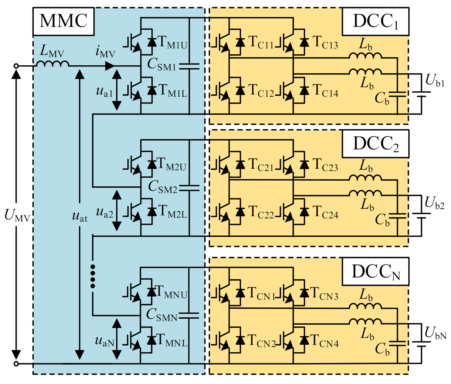
In this paper, a cascaded MMC–BDC is studied, which is shown in Figure 1. The duplicate chopping circuit (DCC) is cascaded at the modular multilevel converter (MMC) sub-module capacitor, which connects the distributed energy storage elements. In the next generation of vessel integrated power systems, the MVDC bus, which is indicated by U_MV, is supplied by multi-phase rectified generators.

In Figure 1, U_MV and i_MV are DC voltage and DC current at the MVDC side, U_bi (i = 1, …, N) is the voltage of ith energy storage element, u_ai is the voltage generated at the MVDC side by the half bridge sub-modules, and u_at is the sum of these. T_miu and T_mid are IGBTs of MMC, T_D11~T_D14, …, T_DN1~T_DN4 are IGBTs of DCCs, L_MV is the filtering inductor at the MVDC side, C_SM is the capacitor of the MMC sub module, and L_b and C_b are filtering inductors and filtering capacitors of DCC, respectively.

According to the characteristics of the inductor and capacitor, one obtains:

$$\begin{array}{l}{L}_{\mathrm{MV}}\frac{d{i}_{\mathrm{MV}}}{dt}=U_{\mathrm{MV}}-{\displaystyle \sum _{i=1}^N{d^{\prime }}_{\mathrm{M}i}{u}_{\mathrm{SM}i}}\\ C_{\mathrm{SM}}\frac{d{u}_{\mathrm{SM}i}}{dt}={d^{\prime }}_{\mathrm{M}i}{i}_{\mathrm{MV}}-\frac{P_{\mathrm{SM}i}}{u_{\mathrm{SM}i}}\end{array}$$

(1)

where, i = 1, …, N, u_SMi is the capacitor voltage of ith MMC sub-module, and d′_Mi is the duty ratio of upper IGBTs of MMC. Supposing that the ripple of i_MV and u_SMi can be neglected, and letting the left side of the first formula of the equation be 0, we obtain:

$$U_{\mathrm{MV}}={\displaystyle \sum _{i=1}^N{d^{\prime }}_{\mathrm{M}i}{u}_{\mathrm{SM}i}}$$

(2)

It can be seen that the sum of the product of the sub-module voltage and the corresponding upper IGBT duty ratio is fixed, which equals the MVDC bus voltage. Letting the left side of the second equation of (1) be 0, we obtain the expression of the sub-module power:

$$P_{\mathrm{SM}i}={d^{\prime }}_{\mathrm{M}i}{u}_{\mathrm{SM}i}{i}_{\mathrm{MV}}$$

(3)

from which, the expression of the sub-module power ratio, or so-called power imbalance degree, can be deduced as:

$${\delta }_i\triangleq \frac{P_{\mathrm{SM}i}}{P_{\mathrm{tot}}}=\frac{{d^{\prime }}_{\mathrm{M}i}{u}_{\mathrm{SM}i}}{{\displaystyle \sum _{i=1}^N{d^{\prime }}_{\mathrm{M}i}{u}_{\mathrm{SM}i}}}=\frac{{d^{\prime }}_{\mathrm{M}i}{u}_{\mathrm{SM}i}}{U_{\mathrm{MV}}}$$

(4)

It can be seen that, as the duty ratio of the upper IGBT and the sub-module voltage are both restricted, the imbalance degree is also limited. In this paper, this limitation is called the imbalance boundary of MMC–BDC. For a more detailed discussion of the imbalance degree, one can refer to [9]. Under different control strategies, the boundary is different.

In the normal operation of MMC–BDC, the sub-module power is evenly distributed, which means δ_i = 1/N (i = 1, 2, …, N). However, as has been noted in Section 1, in the application of vessel integrated power systems many factors can result in the unbalanced distribution of SOC of the distributed energy storage elements. In order to balance the SOC level, inconsistent sub-module power should be conducted in MMC–BDC. When charging the energy storage elements, in order to balance the unbalanced SOC levels, the charging power reference for the low-SOC element should be larger than the high-SOC element. On the contrary, when discharging the energy storage elements, the discharging power reference for the low-SOC element should be smaller than the high-SOC element. For example, when the SOC levels are 30%, 50%, 50% and 50%, respectively, if we want to balance the SOC in the charging ways, we should set the power reference for the first element larger than that of the other three ones. The specific difference in the references is a degree of control freedom. As long as P_SM1 > P_SMi (i = 2, 3, 4), the SOC level can be balanced.

3. Traditional Control Strategies

This section analyzes the imbalance boundary and the voltage stress of components under two traditional control strategies for MMC–BDC featuring different types of sub-module voltage control, which are common voltage control strategies (CVCS) and independent voltage control strategies (IVCS). In the independent voltage control strategy, the sub-module voltage is controlled by DCC, so it is abbreviated as DCC-driven IVCS.

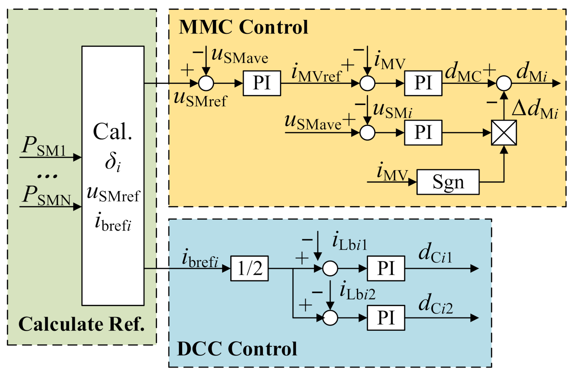
3.1. Common Voltage Control Strategy

Under CVCS, the sub-module voltage of MMC is controlled identically. The block diagram of CVCS is shown in Figure 2. In the CVCS, MMC is used to control the sub-module capacitor voltage u_SMi, and DCC is responsible for controlling the charging and discharging current of the energy storage element. MMC controls the average voltage of the sub-module capacitors u_SMave through double-loop PI control, where the control variable of the inner loop is the MVDC side current i_MV. The output of the double-loop control d_MC is consistent for all sub-modules. Additionally, the voltage balancing is achieved through a single-loop PI control. The positive or negative of Δd_Mi is determined according to the direction of i_MV. Single-loop PI current control is adopted by each phase of DCC.

The calculation of the sub-module voltage reference is given as:

$$u_{\mathrm{SMref}}=\left\{\begin{array}{l}\min \left(u_{\mathrm{SM}}\right)\hspace{1em}\hspace{1em}\hspace{1em}{\delta }_{\max }\le {\delta }_{\mathrm{s}0}\\ {\delta }_{\max }{U}_{\mathrm{MV}}\hspace{1em}\hspace{1em}{\delta }_{\mathrm{s}0}\le {\delta }_{\max }\le {\delta }_{\mathrm{s}1}\end{array}\right.$$

(5)

where, δ_S0 = min(u_SM)/U_MV, which is the maximum imbalance degree corresponding to minimum sub-module voltage min(u_SM). The sub-module voltage is clamped by the DCC diodes, so that min(u_SM) ≥ max(U_bi). In addition, in order to realize the volt–second balance of the MVDC side inductor, min(u_SM) ≥ U_MV/N. Thus, the minimum sub-module voltage of MMC–BDC under CVCS is obtained as:

$$\min \left(u_{\mathrm{SM}}\right)=\max \left[\max \left(U_{\mathrm{b}i}\right),\frac{U_{\mathrm{MV}}}{N}\right]$$

(6)

δ_S1 = max(u_SM)/U_MV, which is the maximum imbalance degree under maximum sub-module voltage. max(u_SM) is determined by the maximum withstanding voltage capability of the components.

According to (4), the imbalance boundary of CVCS can be deduced from the range of duty ratio and sub-module voltage. The range of the upper IGBT duty ratio is (0,1). The range of sub-module voltage is:

$$\max \left[\max \left(U_{\mathrm{b}i}\right),\frac{U_{\mathrm{MV}}}{N}\right]\le u_{\mathrm{SM}}\le \max \left(u_{\mathrm{SM}}\right)$$

(7)

Therefore, the imbalance boundary of CVCS is obtained as:

$$0\le {\delta }_i\le \frac{\max \left(u_{\mathrm{SM}}\right)}{U_{\mathrm{MV}}}$$

(8)

Only when the imbalance degrees of all N sub-modules satisfy (8) can the converter find the steady-state operation point.

Under CVCS, when δ_s0 ≤ δ_max ≤ δ_S1, according to (5), the voltage stress of all sub-modules is determined by the sub-module with the largest power imbalance degree, which can be expressed as:

$$\mathrm{str}\left(u_{\mathrm{SM}i}\right)=U_{\mathrm{MV}}\max \left({\delta }_i\right),\hspace{1em}\left(i=1,\dots ,N\right)$$

(9)

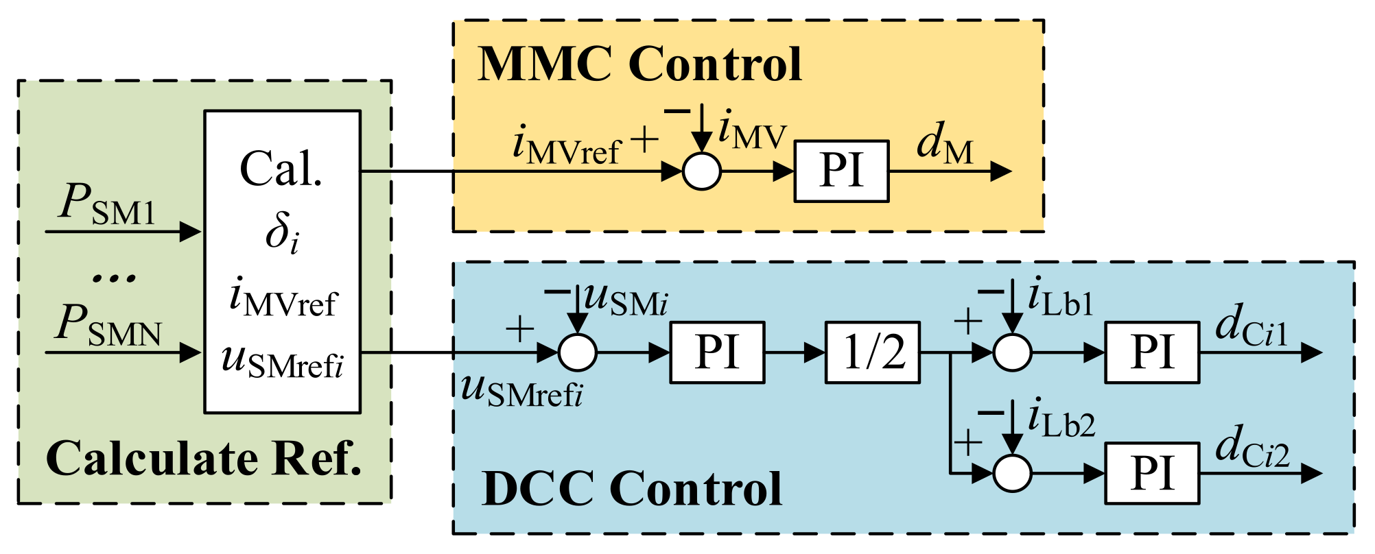
3.2. DCC-Driven Independent Voltage Control Strategy

Under DCC-driven IVCS, the sub-module voltage is controlled independently by DCCs. The block diagram is shown as Figure 3. MMC controls the MVDC side current, which reflects the total power, while DCC controls the sub-module voltages. This control strategy adopts common duty ratio controls in MMC. In order to reduce the voltage stress, when designing the sub-module voltage references of DCC, the voltage reference is chosen to make the duty ratios of all sub-modules of MMC be 1 (there will be a margin in practical application, such as 0.9).

The calculation of the sub-module voltage reference is expressed as:

$$u_{\mathrm{SMref}i}={\delta }_i{U}_{\mathrm{MV}}\hspace{1em}\hspace{1em}{\delta }_{\mathrm{s}0}\le {\delta }_i\le {\delta }_{\mathrm{s}1}$$

(10)

In this case, δ_S0 = min(u_SMi)/U_MV, which corresponds to the imbalance degree corresponding to the minimum allowed voltage of the ith sub-module. The minimum sub-module voltage is constrained by the corresponding energy storage element, which may be different. δ_S1 = max(u_SMi)/U_MV is the imbalance degree corresponding to the maximum allowed voltage of the ith sub module. Generally, δ_S1 is consistent for each sub-module.

It can be seen that under the DCC-driven IVCS, in order to reduce the voltage stress of the sub-modules, the duty ratio of the upper IGBT of the MMC is controlled at 1. Then, according to (4), the distribution of the imbalance degree is only related to the sub-module voltage. Under DCC-driven IVCS, the minimum value of sub module voltage can be less than U_MV/N under the condition that:

$${\displaystyle \sum _{i=1}^N{u}_{\mathrm{SM}i}}\ge U_{\mathrm{MV}}$$

(11)

min(u_SMi) is still clamped by DCC, so the range of sub-module voltage is:

$$U_{\mathrm{b}i}\le u_{\mathrm{SM}i}\le \max \left(u_{\mathrm{SM}}\right)$$

(12)

Hence, the imbalance boundary of DCC-driven IVCS should be:

$$\frac{U_{\mathrm{b}i}}{U_{\mathrm{MV}}}\le {\delta }_i\le \frac{\max \left(u_{\mathrm{SM}}\right)}{U_{\mathrm{MV}}}$$

(13)

Under DCC-driven IVCS, when δ_s0 ≤ δ_i ≤ δ_S1 for all sub-modules, the voltage stress of each sub-module is determined by their own imbalance degree, which can be expressed as:

$$\mathrm{str}\left(u_{\mathrm{SM}i}\right)=U_{\mathrm{MV}}{\delta }_i,\hspace{1em}\left(i=1,\dots ,N\right)$$

(14)

Since the switching loss of MMC is approximately proportional to the sub-module voltage, the ratio of the switching loss of MMC under DCC-driven IVCS to that under CVCS can be calculated as:

$$\mu =\frac{{\displaystyle \sum _{i=1}^N{\delta }_i}}{N\max \left({\delta }_i\right)}=\frac{1}{N\max \left({\delta }_i\right)}$$

(15)

3.3. Problems of the Existing Strategies

Comparing the above two methods, the imbalance boundary of CVCS is larger, but the efficiency is lower. The DCC-driven IVCS reduces the voltage stress of the less unbalanced sub-modules, but its imbalance boundary is more constrained due to the limitation of the sub-module voltage. Therefore, this paper proposes an MMC-driven independent voltage control strategy (MMC-driven IVCS) where MMC controls the sub-module voltage, aiming at good performance both in efficiency and at the imbalance boundary.

4. MMC-Driven IVCS

According to the characteristics of MMC, the feedback linearization control strategy proposed in [23] is improved in this paper. Different from [23], the integral term is introduced in the control law of this paper to overcome the error caused by the inaccuracy of the model. Using the proposed method, the decoupling control of the voltage of each MMC sub-module can be realized, and the maximum imbalance boundary operation can be realized. In addition, the proposed method can make the dynamic characteristics of sub-module voltage symmetrical.

4.1. Internal Dynamic of MMC

According to (1), there are (N + 1) state variables in the MMC model, which are N sub-module capacitor voltages and the MVDC inductor current, which indicates that the system order of MMC is (N + 1). It can be seen that the relative order of each sub-module voltage is 1. Therefore, if we choose the N sub-module voltages as the control output in the feedback linearization, the total relative order N is smaller than the system order (N + 1), and the MVDC current is the internal dynamic variable. We should first justify if the internal dynamic is stable.

Assuming that all the controlled state variables (all the sub-module voltages) have been controlled to the target values, according to (1), the steady-state duty ratios are:

$$d_{\mathrm{M}i}=1-\frac{P_{\mathrm{SM}i}}{i_{\mathrm{MV}}{u}_{\mathrm{SM}i}}$$

(16)

where, i = 1, 2, …, N. Substituting (16) into the inductor current state equation in (1), we obtain:

$$L_{\mathrm{MV}}\frac{d{i}_{\mathrm{MV}}}{dt}=U_{\mathrm{MV}}-\frac{P_{\mathrm{tot}}}{i_{\mathrm{MV}}}=-\frac{U_{\mathrm{MV}}\left(i_{\mathrm{MVref}}-i_{\mathrm{MV}}\right)}{i_{\mathrm{MV}}}$$

(17)

where, i_MVref is the steady-state reference of the MVDC current. Denoting the error of the MVDC inductor current as:

$$e_{\mathrm{I}}=i_{\mathrm{MVref}}-i_{\mathrm{MV}}$$

(18)

(17) can be rewritten as:

$$L_{\mathrm{MV}}{\dot{e}}_{\mathrm{I}}=\frac{U_{\mathrm{MV}}{e}_{\mathrm{I}}}{i_{\mathrm{MV}}}$$

(19)

which shows that the product of the current error and its derivative is positive, illustrating that the internal dynamic is unstable. Hence, MMC is a multi-input-multi-output non-minimum phase nonlinear system.

4.2. Design of Control Law

In order to solve the problem of the unstable internal dynamic, the Lyapunov-based method in [23] is studied and modified in this paper. In the stability analysis of electrical nonlinear systems, the Lyapunov function is often written in the form of reactive component energy. However, in order to introduce the integral term into the control law, the Lyapunov candidate function designed in this paper is:

$$V={\displaystyle \sum _{i=1}^N{V}_{\mathrm{U}i}}+{\displaystyle \sum _{i=1}^N{V}_{\mathrm{IntU}i}}+V_{\mathrm{I}}=\frac{1}{2}{C}_{\mathrm{SM}}{\displaystyle \sum _{i=1}^N{e}_{\mathrm{U}i}^2}+\frac{1}{2}{C}_{\mathrm{SM}}{\displaystyle \sum _{i=1}^N{\gamma }_{\mathrm{IntU}i}{e}_{\mathrm{IntU}i}^2}+\frac{1}{2}{L}_{\mathrm{MV}}{e}_{\mathrm{I}}^2$$

(20)

where, V_Ui, V_IntUi and V_I represent the terms corresponding to the sub-module voltage error e_Ui, the sub-module voltage integral e_IntUi and the MVDC current error e_I in the Lyapunov function, respectively. γ_IntUi is the coefficients of the integral term. Obviously, the above Lyapunov function is no less than 0. After deriving the function, one obtains:

$$\begin{array}{l}{\dot{V}}_{\mathrm{U}i}+{\dot{V}}_{\mathrm{IntU}i}=C_{\mathrm{SM}}{e}_{\mathrm{U}i}\left({\dot{e}}_{\mathrm{U}i}+{\gamma }_{\mathrm{IntU}i}{e}_{\mathrm{IntU}i}\right)\\ {\dot{V}}_{\mathrm{I}}=L_{\mathrm{MV}}{e}_{\mathrm{I}}{\dot{e}}_{\mathrm{I}}\end{array}$$

(21)

In order to calculate the state equation of current error, a reference system is defined:

$$L_{\mathrm{MV}}\frac{d{i}_{\mathrm{MVref}}}{dt}=U_{\mathrm{MV}}-{\displaystyle \sum _{i=1}^N\left(1-d_{\mathrm{M}i\mathrm{ref}}\right)u_{\mathrm{SM}i}}$$

(22)

Subtracting (22) by the first equation of (1), we have:

$$L_{\mathrm{MV}}{\dot{e}}_{\mathrm{I}}={\displaystyle \sum _{i=1}^N{u}_{\mathrm{SM}i}{e}_{\mathrm{Md}i}}$$

(23)

where e_Mdi is the error in the duty ratio. Substitute (23) into Lyapunov function, and:

$$\begin{array}{l}{\dot{V}}_{\mathrm{U}i}+{\dot{V}}_{\mathrm{IntU}i}=C_{\mathrm{SM}}{e}_{\mathrm{U}i}\left({\dot{e}}_{\mathrm{U}i}+{\gamma }_{\mathrm{IntU}i}{e}_{\mathrm{IntU}i}\right)\\ {\dot{V}}_{\mathrm{I}}=e_{\mathrm{I}}{\displaystyle \sum _{i=1}^N{u}_{\mathrm{SM}i}{e}_{\mathrm{d}i}}\end{array}$$

(24)

To make the derivative of V_I not greater than 0, let

$${\displaystyle \sum _{i=1}^N{u}_{\mathrm{SM}i}{e}_{\mathrm{Md}i}}=-{\beta }_{\mathrm{I}}{e}_{\mathrm{I}} \mathrm{where}, {\beta }_1>0$$

(25)

Then,

$${\dot{V}}_{\mathrm{I}}=-{\beta }_{\mathrm{I}}{e}_{\mathrm{I}}^2\le 0$$

(26)

In Equation (22), if the derivative of the MVDC current reference is considered small, then:

$${\displaystyle \sum _{i=1}^N{u}_{\mathrm{SM}i}{d}_{\mathrm{M}i\mathrm{ref}}}={\displaystyle \sum _{i=1}^N{u}_{\mathrm{SM}i}}-U_{\mathrm{MV}}$$

(27)

Then subtract (25) by (27):

$${\displaystyle \sum _{i=1}^N{u}_{\mathrm{SM}i}{d}_{\mathrm{M}i}}={\displaystyle \sum _{i=1}^N{u}_{\mathrm{SM}i}}-U_{\mathrm{MV}}+{\beta }_{\mathrm{I}}{e}_{\mathrm{I}}$$

(28)

When the control input meets the above equation, i_MV can be stable if the control variable d_M1~d_M(N−1) is set through the partial feedback linearization method [21], which is:

$$\begin{array}{l}{d}_{\mathrm{M}i}=-\frac{C_{\mathrm{SM}}}{i_{\mathrm{MV}}}{v}_i+1-\frac{P_{\mathrm{SM}i}}{i_{\mathrm{MV}}{u}_{\mathrm{SM}i}}\\ v_i={\alpha }_{\mathrm{U}i}{e}_{\mathrm{U}i}+{\gamma }_{\mathrm{IntU}i}{e}_{\mathrm{IntU}i}\end{array}$$

(29)

where, v_i is the auxiliary control input. which determines the dynamics of the control output after linearization. Under partial feedback linearization control, the dynamics of the first (N − 1) sub-module voltages can be expressed as follows:

$${\dot{e}}_{\mathrm{U}i}+{\alpha }_{\mathrm{U}i}{e}_{\mathrm{U}i}+{\gamma }_{\mathrm{IntU}i}{e}_{\mathrm{IntU}i}=0$$

(30)

which is a typical second-order system. Combining (30) and (21), the derivative of the Lyapunov functions of the error of the sub-module voltage and the integral can be obtained as:

$${\dot{V}}_{\mathrm{U}i}+{\dot{V}}_{\mathrm{IntU}i}=C_{\mathrm{SM}}{e}_{\mathrm{U}i}{\dot{e}}_{\mathrm{U}i}+{\gamma }_{\mathrm{IntU}i}{C}_{\mathrm{SM}}{e}_{\mathrm{U}i}{e}_{\mathrm{IntU}i}=-{\alpha }_{\mathrm{U}i}{C}_{\mathrm{SM}}{e}_{\mathrm{U}i}^2$$

(31)

which indicates that the term corresponding to the integral of the error of the first (N − 1) sub-module voltages can be eliminated, and the final result is not greater than 0.

Combining (29) into (28) we obtain:

$$d_{\mathrm{MN}}=1-\frac{U_{\mathrm{MV}}}{u_{\mathrm{SMN}}}+\frac{P_{\mathrm{tot}}-P_{\mathrm{SMN}}}{u_{\mathrm{SMN}}{i}_{\mathrm{MV}}}+\frac{C_{\mathrm{SM}}}{u_{\mathrm{SMN}}{i}_{\mathrm{MV}}}{\displaystyle \sum _{i=1}^{N-1}{u}_{\mathrm{SM}i}\left({\alpha }_{\mathrm{U}i}{e}_{\mathrm{U}i}+{\gamma }_{\mathrm{IntU}i}{e}_{\mathrm{IntU}i}\right)}+\frac{{\beta }_{\mathrm{I}}}{u_{\mathrm{SMN}}}{e}_{\mathrm{I}}$$

(32)

By substituting d_MN into the term corresponding to the Nth sub-module voltage in the Lyapunov function, we obtain:

$$\begin{array}{ll}{\dot{V}}_{\mathrm{UN}}+{\dot{V}}_{\mathrm{IntUN}}& =C_{\mathrm{SM}}{e}_{\mathrm{UN}}\left({\dot{e}}_{\mathrm{UN}}+{\gamma }_{\mathrm{IntUN}}{e}_{\mathrm{IntUN}}\right)=e_{\mathrm{UN}}\left[\frac{P_{\mathrm{SMN}}}{u_{\mathrm{SMN}}}-\left(1-d_{\mathrm{MN}}\right)i_{\mathrm{MV}}\right]+C_{\mathrm{SM}}{\gamma }_{\mathrm{IntUN}}{e}_{\mathrm{UN}}{e}_{\mathrm{IntUN}}\\ \hspace{1em}& =\frac{e_{\mathrm{UN}}}{u_{\mathrm{SMN}}}\left[P_{\mathrm{tot}}-U_{\mathrm{MV}}{i}_{\mathrm{MV}}+{\beta }_{\mathrm{I}}{i}_{\mathrm{MV}}{e}_{\mathrm{I}}+C_{\mathrm{SM}}{\displaystyle \sum _{i=1}^{N-1}{\alpha }_{\mathrm{U}i}{u}_{\mathrm{SM}i}{e}_{\mathrm{U}i}}+C_{\mathrm{SM}}{\displaystyle \sum _{i=1}^N{\gamma }_{\mathrm{IntU}i}{u}_{\mathrm{SM}i}{e}_{\mathrm{IntU}i}}\right]\end{array}$$

(33)

Assuming that the regulation of the MVDC current i_MV is much faster than that of the sub-module capacitor voltage, then:

$$i_{\mathrm{MV}}=i_{\mathrm{MVref}},e_{\mathrm{I}}=0$$

(34)

Consequently:

$${\dot{V}}_{\mathrm{UN}}+{\dot{V}}_{\mathrm{IntUN}}=\frac{e_{\mathrm{UN}}}{u_{\mathrm{SMN}}}\left[P_{\mathrm{tot}}-U_{\mathrm{MV}}{i}_{\mathrm{MVref}}+C_{\mathrm{SM}}{\displaystyle \sum _{i=1}^{N-1}{\alpha }_{\mathrm{U}i}{u}_{\mathrm{SM}i}{e}_{\mathrm{U}i}}+C_{\mathrm{SM}}{\displaystyle \sum _{i=1}^N{\gamma }_{\mathrm{IntU}i}{u}_{\mathrm{SM}i}{e}_{\mathrm{IntU}i}}\right]$$

(35)

As long as:

$$i_{\mathrm{MVref}}=\frac{P_{\mathrm{tot}}}{U_{\mathrm{MV}}}+\frac{C_{\mathrm{SM}}}{U_{\mathrm{MV}}}{\displaystyle \sum _{i=1}^{N-1}{\alpha }_{\mathrm{U}i}{u}_{\mathrm{SM}i}{e}_{\mathrm{U}i}}+\frac{{\beta }_{\mathrm{UN}}}{U_{\mathrm{MV}}}{u}_{\mathrm{SMN}}{e}_{\mathrm{UN}}+\frac{C_{\mathrm{SM}}}{U_{\mathrm{MV}}}{\displaystyle \sum _{i=1}^N{\gamma }_{\mathrm{IntU}i}{u}_{\mathrm{SM}i}{e}_{\mathrm{IntU}i}}$$

(36)

it can be derived that:

$${\dot{V}}_{\mathrm{UN}}+{\dot{V}}_{\mathrm{IntUN}}=-{\beta }_{\mathrm{UN}}{e}_{\mathrm{UN}}^2$$

(37)

which shows the asymptotic stability of the sub-module voltages.

Assuming that:

$${\alpha }_{\mathrm{UN}}=\frac{{\beta }_{\mathrm{UN}}}{C_{\mathrm{SM}}}$$

(38)

the MVDC current reference can be calculated as:

$$i_{\mathrm{MVref}}=\frac{P_{\mathrm{tot}}}{U_{\mathrm{MV}}}+\frac{C_{\mathrm{SM}}}{U_{\mathrm{MV}}}{\displaystyle \sum _{i=1}^N{\alpha }_{\mathrm{U}i}{u}_{\mathrm{SM}i}{e}_{\mathrm{U}i}}+\frac{C_{\mathrm{SM}}}{U_{\mathrm{MV}}}{\displaystyle \sum _{i=1}^N{\gamma }_{\mathrm{IntU}i}{u}_{\mathrm{SM}i}{e}_{\mathrm{IntU}i}}$$

(39)

Overall, the proposed Lyapunov-function-based feedback linearization control law is summarized as:

$$\begin{array}{l}{d}_{\mathrm{M}i}=-\frac{C_{\mathrm{SM}}}{i_{\mathrm{MV}}}{v}_i+1-\frac{P_{\mathrm{SM}i}}{i_{\mathrm{MV}}{u}_{\mathrm{SM}i}} \mathrm{where}, v_i={\alpha }_{\mathrm{U}i}{e}_{\mathrm{U}i}+{\gamma }_{\mathrm{IntU}i}{e}_{\mathrm{IntU}i}\\ d_{\mathrm{MN}}=1-\frac{U_{\mathrm{MV}}}{u_{\mathrm{SMN}}}+\frac{P_{\mathrm{tot}}-P_{\mathrm{SMN}}}{u_{\mathrm{SMN}}{i}_{\mathrm{MV}}}+\frac{C_{\mathrm{SM}}}{u_{\mathrm{SMN}}{i}_{\mathrm{MV}}}{\displaystyle \sum _{i=1}^{N-1}{u}_{\mathrm{SM}i}\left({\alpha }_{\mathrm{U}i}{e}_{\mathrm{U}i}+{\gamma }_{\mathrm{IntU}i}{e}_{\mathrm{IntU}i}\right)}+\frac{{\beta }_{\mathrm{I}}}{u_{\mathrm{SMN}}}{e}_{\mathrm{I}} \mathrm{where}, e_{\mathrm{I}}=i_{\mathrm{MV}}^R-i_{\mathrm{MV}}\end{array}$$

(40)

4.3. Dynamic Analysis and Control Parameter Design

As is known from (26), the dynamic characteristic of i_MV is:

$$L_{\mathrm{MV}}{\dot{e}}_{\mathrm{I}}+{\beta }_{\mathrm{I}}{e}_{\mathrm{I}}=0$$

(41)

which is a typical first-order system. Assuming that

$${\alpha }_{\mathrm{I}}=\frac{{\beta }_{\mathrm{I}}}{L_{\mathrm{MV}}}$$

(42)

Then:

$${\dot{e}}_{\mathrm{I}}+{\alpha }_{\mathrm{I}}{e}_{\mathrm{I}}=0$$

(43)

Assuming the cut-off frequency to be f_CI, the control parameter should be:

$${\alpha }_{\mathrm{I}}=2\pi f_{\mathrm{cI}}$$

(44)

According to (30), the dynamic of the first (N − 1) sub-module voltage is:

$${\ddot{e}}_{\mathrm{U}i}+{\alpha }_{\mathrm{U}i}{\dot{e}}_{\mathrm{U}i}+{\gamma }_{\mathrm{IntU}i}{e}_{\mathrm{U}i}=0$$

(45)

where i = 1, 2, …, N − 1. According to (37) and (38), the dynamic of the Nth sub-module voltage can be obtained as:

$${\dot{e}}_{\mathrm{UN}}+{\alpha }_{\mathrm{UN}}{e}_{\mathrm{UN}}+{\gamma }_{\mathrm{IntUN}}{e}_{\mathrm{IntUN}}=0$$

(46)

In order to make the dynamics of each sub-module voltage similar, we should make:

$$\begin{array}{l}{\alpha }_{\mathrm{U}1}={\alpha }_{\mathrm{U}2}=\dots ={\alpha }_{\mathrm{UN}}={\alpha }_{\mathrm{U}}\\ {\gamma }_{\mathrm{IntU}1}={\gamma }_{\mathrm{IntU}2}=\dots ={\gamma }_{\mathrm{IntUN}}={\gamma }_{\mathrm{IntU}}\end{array}$$

(47)

Setting the damping ratio to be ξ and the natural oscillation frequency to be f_cU, the control parameters can be designed as:

$$\begin{array}{l}{\alpha }_{\mathrm{U}}=2\xi \sqrt{{\gamma }_{\mathrm{IntU}}}\\ {\gamma }_{\mathrm{IntU}}={\left(2\pi f_{\mathrm{cU}}\right)}^2\end{array}$$

(48)

According to the above analysis, the proposed Lyapunov-function-based feedback linearization control strategy can realize the decoupling control of each state variable, and ensure the symmetry of dynamics of the N sub-module voltages.

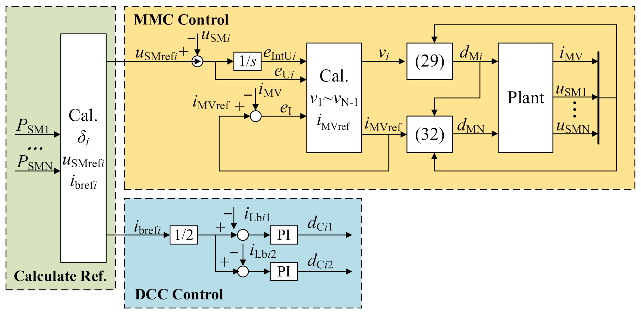
4.4. Imbalance Boundary and Voltage Stress Analysis

The complete block diagram of MMC-driven IVCS is shown in Figure 4. The independent voltage reference can be given as:

$$u_{\mathrm{SMref}i}=\left\{\begin{array}{l}\min \left(u_{\mathrm{SM}i}\right)\hspace{1em}\hspace{1em}{\delta }_i\le {\delta }_{\mathrm{s}0}\\ {\delta }_i{U}_{\mathrm{MV}}\hspace{1em}\hspace{1em}{\delta }_{\mathrm{s}0}\le {\delta }_i\le {\delta }_{\mathrm{s}1}\end{array}\right.$$

(49)

The definition of δ_s0 and δ_S1 is the same as the DCC-driven IVCS. The difference between MMC-driven IVCS and DCC-driven IVCS is that the imbalance boundary of MMC-driven IVCS is wider due to the more adjustable duty ratio.

Under MMC-driven IVCS, the range of duty ratio is (0,1), and the range of the sub-module voltage is:

$$U_{\mathrm{b}i}\le u_{\mathrm{SM}i}\le \max \left(u_{\mathrm{SM}}\right)$$

(50)

So, the imbalance boundary is:

$$0\le {\delta }_i\le \frac{\max \left(u_{\mathrm{SM}}\right)}{U_{\mathrm{MV}}}$$

(51)

Under MMC-driven IVCS, when δ_s0 ≤ δ_S1, the voltage stress of each sub-module is determined by their own imbalance degree, which can be expressed as:

$$\mathrm{str}\left(u_{\mathrm{SM}i}\right)=U_{\mathrm{MV}}{\delta }_i/{d^{\prime }}_{\mathrm{M}i},\hspace{1em}\left(i=1,\dots ,N\right)$$

(52)

According to the voltage stress, the ratio of the switching loss of MMC under MMC-driven IVCS to that under CVCS can be calculated as:

$$\mu =\frac{{\displaystyle \sum _{i=1}^N{\delta }_i}}{N\max \left({\delta }_i\right)}=\frac{1}{N\max \left({\delta }_i\right)}$$

(53)

which is the same as the DCC-driven IVCS.

Obviously, the proposed MMC-driven IVCS combines the advantages of CVCS and DCC-driven IVCS. It not only has a wide imbalance boundary, but also has a high operating efficiency. The characteristics of the three strategies are shown in

Table 1. Comparisons of the three kinds of control strategies.

Strategy	Imbalance Boundary	MMC Switching Loss Ratio
CVCS	$0\le {\delta }_i\le \frac{\max \left(u_{\mathrm{SM}}\right)}{U_{\mathrm{MV}}}$	1
DCC-driven IVCS	$\frac{U_{\mathrm{b}i}}{U_{\mathrm{MV}}}\le {\delta }_i\le \frac{\max \left(u_{\mathrm{SM}}\right)}{U_{\mathrm{MV}}}$	$\mu =\frac{1}{N\max \left({\delta }_i\right)}$
MMC-driven IVCS	$0\le {\delta }_i\le \frac{\max \left(u_{\mathrm{SM}}\right)}{U_{\mathrm{MV}}}$	$\mu =\frac{1}{N\max \left({\delta }_i\right)}$

.

In the practical application, in order to leave some margin for duty ratio regulation, the voltage reference of the sub-module is set as:

$$u_{\mathrm{SMref}i}=\left\{\begin{array}{l}\min \left(u_{\mathrm{SM}i}\right)\hspace{1em}\hspace{1em}{\delta }_i\le {\delta }_{\mathrm{s}0}\\ {\delta }_i{U}_{\mathrm{MV}}/0.8\hspace{1em}{\delta }_{\mathrm{s}0}\le {\delta }_i\le {\delta }_{\mathrm{s}1}\end{array}\right.$$

(54)

where the steady-state lower IGBT duty ratio is 0.8 instead of 1.

Additionally, as can be inferred from the control law in (40), the control system is at its singular point when i_MV = 0. Hence, in the actual application, the MMC–BDC is started up under CVCS, and then switched into MMC-driven IVCS.

5. Simulation Verification

The parameters of the MMC–BDC prototype studied in this paper can be referred to in

Table 2. Parameters of the MMC–BDC prototype.

Parameter	Value
Number of sub-modules N	4
MVDC side inductor LMV (mH)	4
Sub-module capacitor CSM (mF)	0.6
MVDC bus voltage UMV (V)	850
Maximum allowed sub-module voltage (V)	380
Minimum allowed sub-module voltage (V)	300
Switching frequency fs (Hz)	5000

.

According to Section 4, the imbalance boundary of CVCS, DCC-driven IVCS and MMC-driven IVCS in this case is (0,0.4471), (0.1412,0.4471) and (0,0.4471). Compared with DCC-driven IVCS, the imbalance boundary of the proposed method is increased by 31.58%.

In consideration of the 5 kHz switching frequency, the control parameters are designed as in

Table 3. Control parameters of the case study.

Parameter	Value
αI	1800
αU	125
γIntU	8000

.

To test the proposed unbalanced operation control strategy, the power reference of the sub-modules, which is also the power reference of DCC, is given in a stepwise manner, which is shown in Table 4. In this case study, the SOC level of all the four energy storage elements are assumed as 30%, 50%, 50% and 50%, and the rated quantity of electricity of each ESE is set at 200 C to see the changes in the SOC level.

Table 4. Stepwise sub-module power reference.

Stage	PSM1 (W)	PSM2 (W)	PSM3 (W)	PSM4 (W)
I	900	900	900	900
II	1200	900	900	900
III	1350	900	900	900
IV	1500	900	900	900

Under the power reference shown in Table 4, considering the voltage reference shown in (54), the theoretical steady-state sub-module voltage of each stage can be listed as Table 5.

Table 4. Stepwise sub-module power reference.

Stage	PSM1 (W)	PSM2 (W)	PSM3 (W)	PSM4 (W)
I	900	900	900	900
II	1200	900	900	900
III	1350	900	900	900
IV	1500	900	900	900

Under the power reference shown in Table 4, considering the voltage reference shown in (54), the theoretical steady-state sub-module voltage of each stage can be listed as Table 5.

Table 5. Corresponding sub-module voltage reference.

Stage	uSM1 (W)	uSM2 (W)	uSM3 (W)	uSM4 (W)
I	300	300	300	300
II	326	300	300	300
III	354	300	300	300
IV	379	300	300	300

Table 5. Corresponding sub-module voltage reference.

Stage	uSM1 (W)	uSM2 (W)	uSM3 (W)	uSM4 (W)
I	300	300	300	300
II	326	300	300	300
III	354	300	300	300
IV	379	300	300	300

According to Section 4, the MMC switching loss ratios of the four stages are (1,0.8125,0.75,0.7), respectively. The improvement of the imbalance boundary and MMC switching loss ratios is summarized in

Table 6. The indicator improvement of MMC-driven IVCS.

Indicators		CVCS	DCC-Driven IVCS	MMC-Driven IVCS
Imbalance boundary		[0,0.4471]	[0.1412,0.4471]	[0.1412,0.4471]
MMC switching loss ratio	Stage I	1	1	1
	Stage II	1	0.8125	0.8125
	Stage III	1	0.75	0.75
	Stage IV	1	0.7	0.7

.

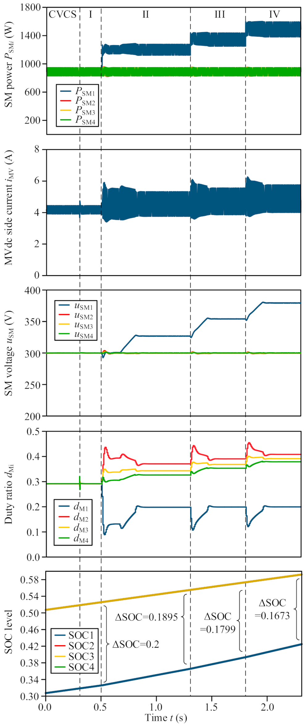
In the simulation, the operation mode of MMC is switched from CVCS to MMC-driven IVCS in 0.3 s. At 0.5 s, the power reference of the first sub-module is switched from 900 W to 1200 W. At 1.3 s, the power command is further changed to 1350 W. At 1.8 s, the last power reference switchover is implemented and the operation enters Stage IV. The simulation waveforms are shown in Figure 5.

The following conclusion can be drawn from Figure 5.

• At 0.3 s, when the control strategy is switched from CVCS to MMC-driven IVCS, there is no obvious fluctuations in the waveforms. This is because the error terms in the control law (36) are close to zero under CVCS. The system can enter the steady-state operation point of MMC-driven IVCS directly. In practical application, due to the uncertainty or inaccuracy of the parameters, it may need to go through a short adjustment process.
• At 0.5 s, the power command of the first sub-module is 1 to 1200 W. According to (50), the voltage reference of the first sub-module is 326 V. Because of ramp setting of the power command, the sub-module voltage reference starts to exceed the initial value of 300 V at about 0.66 s, and the total regulation process takes about 0.5 s. From the slope waveform of the sub-module voltage, the proposed control strategy has good tracking performance.
• At 1.3 s, the power command of the first sub-module is increased to 1350 W. The voltage reference of sub-module voltage increases to 354 V accordingly. The adjustment process takes about 0.15 s. Finally, at 1.8 s, the power command of the first sub-module is changed to 1500 W. The sub-module voltage reference is 379 v. Additionally, the adjustment process takes about 0.16 s.
• The MVDC current ripple increases. This is because the unbalanced operation of MMC results in the unbalanced distributed duty ratios, which ruins the equivalent frequency multiplying effect of the phase-shifted modulation of MMC, which is out of the scope of this paper.
• In the last sub-figure in Figure 5, the initial SOC level is (0.3,0.5,0.5,0.5). At 0.3 s, the SOC level is (0.3185,0.5185,0.5185,0.5185). While at 0.5 s, the SOC distribution is (0.3259,0.5259,0.5259,0.5259). Before 0.5 s, all energy storage elements are charged with balanced power, so the change in the SOC level is consistent. At 1.3 s, which is the end of Stage II, the SOC distribution becomes (0.3660,0.5555,0.5555,0.5555). At 1.8 s, which is the end of Stage III, the SOC is (0.3940,0.5739,0.5739,0.5739). At 2.3 s, which is the end of the whole charging process, the SOC distribution is (0.4251,0.5924,0.5924,0.5924). Throughout the unbalanced charging, the difference in the SOC level is reduced from 0.2 to 0.1673 by 16.35%, which shows the effect of our proposed method in balancing the SOC level.

6. Conclusions

Aiming at the unbalanced operation of MMC–BDC, a feedback linearization control strategy based on Lyapunov function is proposed to realize the independent control of MMC sub-module capacitor voltage. Compared with the traditional MMC–BDC unbalanced operation control strategy, the proposed control strategy has wider imbalance boundary and higher operation efficiency. Compared with the traditional feedback linearization control strategy, the proposed strategy gifts each sub-module voltage symmetrical dynamics. The control law acts directly on the state trajectory of the sub-module voltage, rather than on the virtual control output. In the paper, the control law is derived in detail and compared with the existing unbalanced operation control strategy. Simulation verification is implemented. In the studied case, compared with traditional independent voltage control, the imbalance boundary of the proposed method is increased by 31.58%. Compared with traditional common voltage control, the MMC switching loss of the proposed method is reduced by 30% at most. The simulation result proves the effectiveness of the proposed control strategy.