Minimizing the Computational Effort to Optimize Solar Concentrators with the Open-Source Tools SunPATH and Tonatiuh++

Abstract

Integrals that are of interest in the analysis, design, and optimization of concentrating solar thermal systems (CST), such as the annual optical efficiency of the light collection and concentration (LCC) subsystem, can be accurately computed or estimated in two distinct ways: on the time domain and on the spatial domain. This article explores these two ways, using a case study that is highly representative of the commercial CST systems being deployed worldwide. In the time domain, the computation of these integrals are explored using 1-min, 10-min, and 1-h solar DNI input data and using The Cyprus Institute (CyI)’s High-Performance Computing (HPC) system and an open-source ray tracer, Tonatiuh++, being actively developed at CyI. In the spatial domain, the computation of these integrals is explored using SunPATH, another open-source software tool being actively developed at CyI, in tandem with Tonatiuh++. The comparison between the time and spatial domain approach clearly indicate that the spatial domain approach using SunPATH is dramatically more computationally efficient than the time domain approach. According to the results obtained, at least for the case study analyzed in this article, to compute the annual energy delivered by the LCC subsystem with a relative error less than 0.1%, it is enough to provide SunPATH with 1-h DNI data as input, request from SunPATH the sun position and weights of just 30 points in the celestial sphere, and run Tonatiuh++ to simulate these 30 points using 15 million rays per run. As the test case is highly representative, it is expected that this approach will yield similar results for most CST systems of interest.

1. Introduction

The design of concentrating solar thermal (CST) power system is a complex engineering problem, which requires considerable computational resources. Depending on the approach, the optimization of such systems could involve the optimization of hundreds or even thousands of parameters. The ability to perform the techno-economic optimizations quickly depends on how fast and accurately the annual performance of a CST system or some of their key subsystems can be found [1].

Increasingly, ray tracing is used to model the optical behaviour of the light collection and concentration (LCC) subsystem of CST systems. This technique is one of the most accurate and flexible. It can simulate almost any type of solar concentrator made up of reflecting and refracting surfaces, such as traditional one-reflection heliostat fields, heliostat fields with secondary concentrators and receivers with quartz windows, beam-down systems, parabolic trough reflectors with vacuum glass tube receivers, or linear Fresnel systems with or without non-imaging secondary optics. However, ray tracing is computationally demanding. Because of this, it is of interest to develop approaches to accurately compute the key annual characteristics of a CST system or subsystem, which minimize the number of times a ray tracer has to be run.

Almost all research dealing with the optimization of CST, systems employ approaches to reduce the computational effort needed to estimate annual energy productions or other key annual characteristics, which are based upon numerical interpolation and integration over the sun path [2,3,4]. Such approaches can be based on a simple sampling of a few characteristic days using a fixed time step [5] or on more advanced concepts involving various coordinate transformations and splines [6].

The surface enclosing the annual sun path resembles the shape of a ring on the celestial sphere, the inclination of which depends on the latitude of location [7]. The ring can be described as a parametric surface of two variables, and there are several options for that. A standard choice is to use azimuth and elevation. However, this choice leads to a complicated shape of the interpolation domain and to a singular behavior near the zenith. A better choice is to use declination and hour angle, which produces a trapezoidal domain for all latitudes. In this case, the boundaries corresponding to the winter and summer solstice are always straight as the lines of constant declination. The remaining boundaries for sunrise and sunset are sufficiently close to straight lines for low to medium latitudes. The bivariate interpolation for domains of such shape can be done as a product of two univariate interpolations, and many standards methods like bicubic interpolation can be applied [8].

Note that the accuracy of interpolation depends not only on a particular method, but also on the analytical properties of the function being interpolated. Typically, the optical efficiency of the LCC subsystems of a CST system is a smooth function, and good accuracy can be achieved even for a small number of sampling points [9]. Nevertheless, the use of regular grids for interpolation poses some limitations, and it is hard to adjust the accuracy in regions where the function is known to change more rapidly. For example, the optical efficiency may drop significantly during sunrise and sunset because of shading losses. Irregular grids provide more flexibility in this regard, and the sampling resolution can be adjusted locally. A common approach is to generate a triangular mesh with a variable density and to use a linear interpolation in barycentric coordinates [10]. It is also possible to apply meshless methods based on thin-plate splines or radial basis functions [11]. An important property of meshless methods is that the interpolated function can be represented as a sum of kernels with simple analytical properties. This can be used to simplify various derivations which are necessary for annual integrals and other analysis [12].

This article presents an open-source computer program called SunPATH, being actively developed by the Cyprus Institute, which uses a meshless method for integration over the annual sun path. Inputs to the program are (1) the location being analyzed, (2) the spatial resolution that the user wants to consider, and (3) the values of the solar Direct Normal Irradiance (DNI) at that location at regular time steps over the year. The program’s outputs are (1) the azimuth and elevation of the sampling points and (2) the weights associated to those positions, to be used in estimating the annual integral of any function of sun position and irradiance the user is interested in estimating.

The article also presents a detailed case study to analyze and compare two methods for estimating the annual energy delivered to the receiver by the solar concentrator of a CST system. The first method is based on the numerical integration in the temporal domain. The second method is based on the numerical integration on the spatial domain, assisted by the use of the SunPATH program. Both ways use Tonatiuh++, which is an open-source C++ Monte Carlo Ray Tracer (MCRT), being also actively developed by CyI to estimate the power delivered to the receiver at specific sun positions for specific values of the solar DNI. The analysis of the integration in the temporal domain involves the comparison of the annual estimates obtained using 1-min, 10-min, and 60-min time steps and using two different interpolation approaches. The analysis of the integration in the spatial domain involves the comparison of the annual estimates obtained using 30, 52, and 114 sun positions, and using 1-min, 10-min, and 60-min solar DNI data as input to the SunPATH program.

Finally, the article compares the results obtained in the case study and draws very clear conclusions related to the optimal use of SunPATH (doi:10.5281/zenodo.5116526, accessed on 4 June 2021) and Tonatiuh++ (doi:10.5281/zenodo.5116609, accessed on 4 June 2021) to minimize the computational effort required to estimate key annual characteristics of a CST system, and also what is the influence of the time step in the accuracy of the annual estimates when one is using the temporal domain integration.

Section 2 provides a high-level overview of the mathematical approach used by SunPATH. Section 3 describes the CST system selected for the test case, which is a solar tower very similar to PS10. Section 4 and Section 5 describe the temporal and spatial domain approaches to estimate the annual energy delivered by the heliostat field of the test case CST system to the receiver. Section 6 presents the results of these estimations. Finally, Section 7 summarizes the conclusions and lessons learned, and Section 8 discusses further improvements to the approach presented here that will be explored in the near future.

2. SunPATH Approach to Facilitate Energy Yield Analyses

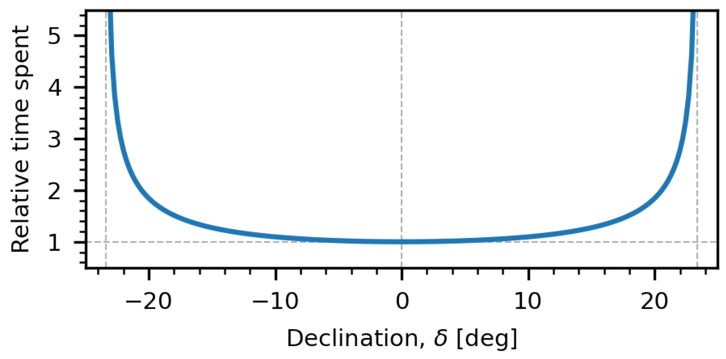
The motion of the sun in the sky can be described with very good accuracy by solving the Kepler’s problem [13]. The solution of this equation shows that the motion of the sun is not uniform. The sun spends different time in different parts of the sky.

For a given location, the set of all positions of the sun during the year along the sun path is contained within a ring-like spherical surface in the celestial sphere. The angle between the axis of symmetry of this ring-like surface and the vertical axis of the location is the latitude of the place. The motion of the sun within this ring-like spherical surface is still a 1D path, which depends on time with a full period of about 4 years. The relative time spent by the sun in a certain solid angle of the ring-like surface containing the sun path strongly depends on the declination of the sun. It can be estimated by using the following relation between the declination $\delta$ and ecliptic longitude $\lambda$:

$$sin\delta =sin{\delta }_{\max }sin\lambda ,$$

(1)

where ${\delta }_{\max }$ is the obliquity of ecliptic. The ecliptic longitude is approximately proportional to time

$$\lambda \approx 2\pi (n-81)/365,$$

(2)

where n is the day number within a year, with day 81 corresponding to the spring equinox. The differentiation of Equation (1) gives

$$cos\delta d\delta =sin{\delta }_{\max }cos\lambda d\lambda ,$$

(3)

or

$$\frac{d\lambda }{d\delta }=\frac{cos\delta }{\sqrt{{sin}^2{\delta }_{\max }-{sin}^2\delta }}.$$

(4)

As $d\lambda$ is proportional to time, the derivative of Equation (1) shows the time spent in the ring of declinations with width $d\delta$. The density grows for large declinations as shown in Figure 1. The singular behaviour at $\delta =\pm {\delta }_{\max }$ corresponds to the turning points at the summer and winter solstices.

In general, the declination changes slowly during a day, and the daily motion of the sun on the celestial sphere resembles a circle with a constant value of $\delta$. The angular separation between the circles for different days $d\delta$ can be computed with Equation (4) by using $d\lambda =2\pi /365=17\mathrm{mrad}$. For equinox $\delta =0$, this gives $d\delta =sin{\delta }_{\max }d\lambda =7\mathrm{mrad}$ or $0.4^{\circ }$, which is comparable to the $0.{52}^{\circ }$ subtended by the sun. This means that as long as we sample the celestial sphere with an angular resolution several times the angle of the sun, e.g., >4.0${}^{\circ }$, we will not have numerical problems or artifacts when defining probability density functions (PDF) related to the time spent by the sun per unit solid angle at locations in the celestial sphere.

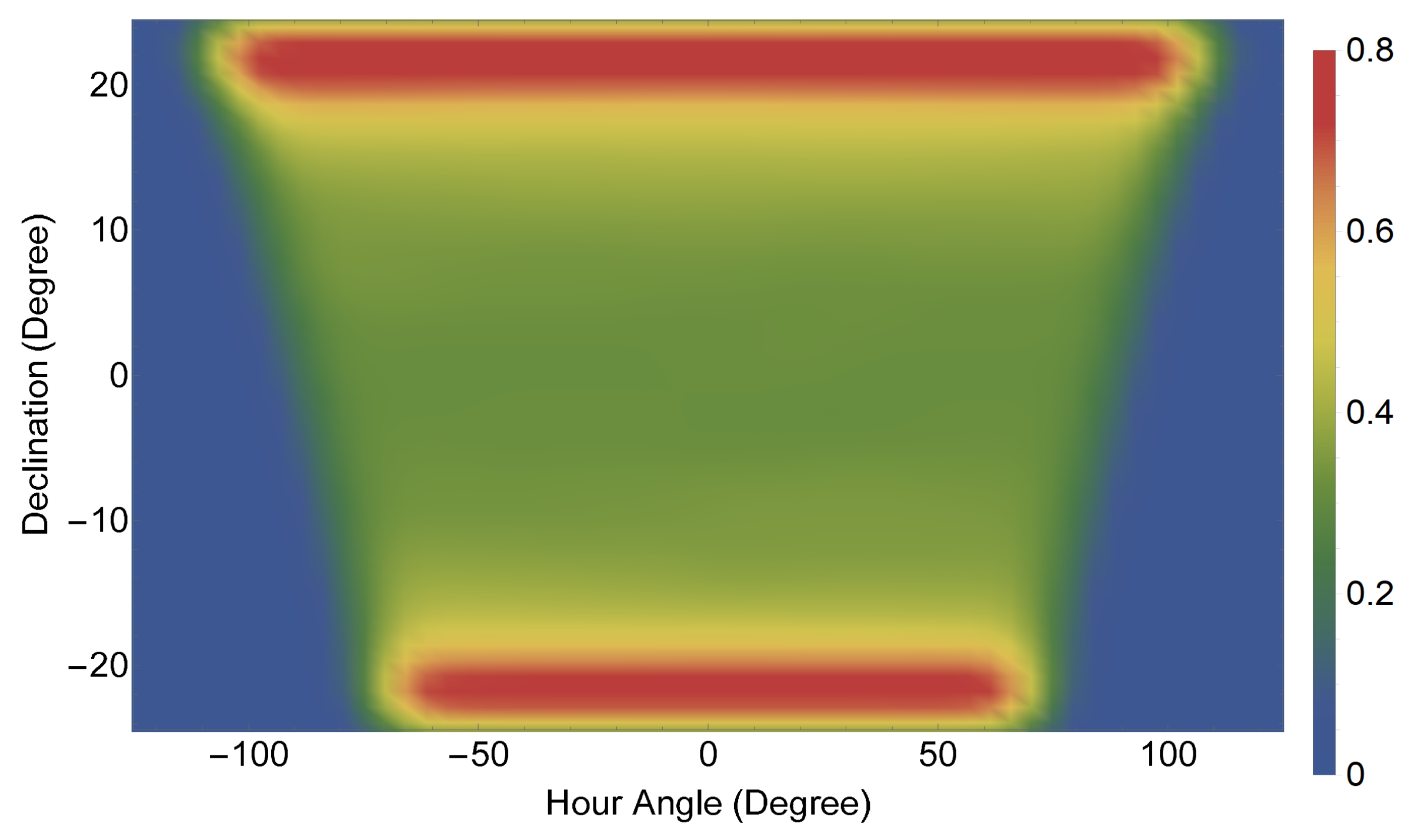
In the spatial domain, the ring-like spherical surface containing the sun path can be parameterized with two variables. A convenient choice of variables are the Sun’s hour angle $\omega$ and declination $\delta$. In these coordinates, the ring-like spherical surface containing the sun path along the year adopts a trapezoidal shape (see Figure 2). The declination of the sun varies in the range $\left|\delta \right|\le ϵ$, where $ϵ=23.4^{\circ }$ is the obliquity of ecliptic. The hour angle changes in the range $\left|\omega \right|\le {\omega }_{\max }\left(\delta \right)$, where

$${\omega }_{\max }\left(\delta \right)=arccos(-tanLtan\delta )$$

(5)

is the hour angle of sunset ($z=0$).

Strictly speaking, the declination for large latitudes $\left|L\right|>{90}^{\circ }-ϵ$ is limited by horizon

$$\max (-ϵ,L-{90}^{\circ })\le \delta \le \min (ϵ,L+{90}^{\circ }),$$

(6)

but the sun path still has a trapezoidal shape.

This shape can be sampled just by taking an equidistant grid of points and stretching it to fit within the boundaries. For example, the sampling of declination interval $\delta \in [{\delta }_{\min },{\delta }_{\max }]$ with the resolution $\rho$ needs $N=\mathrm{round}[({\delta }_{\max }-{\delta }_{\min })/\rho ]$ sub-intervals of the length ${\delta }_{\mathrm{step}}=({\delta }_{\max }-{\delta }_{\min })/N$, and the sampling points can be described as ${\delta }_n={\delta }_{\min }+n{\delta }_{\mathrm{step}}$ with integer $n\in [0,N]$. The hour angles for each declination ${\delta }_n$ can be sampled in a similar way. 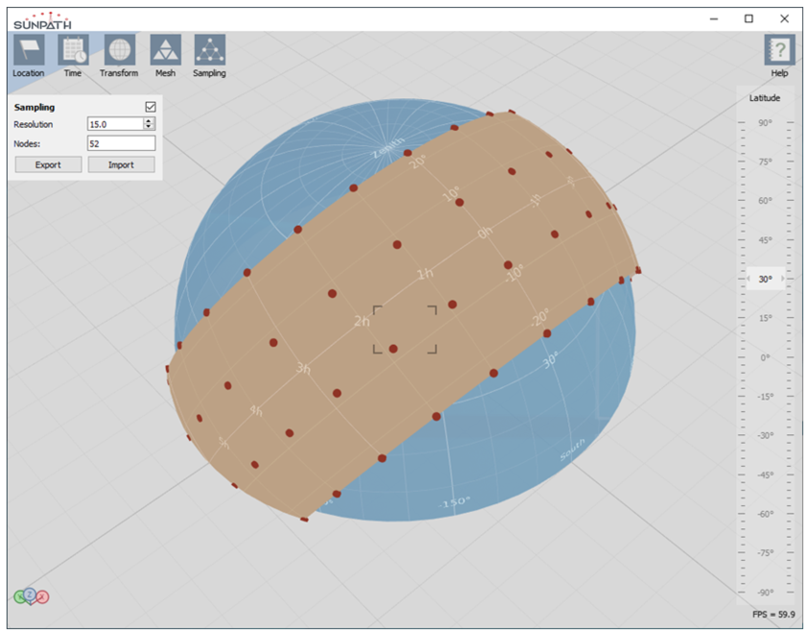Figure 3 presents the Graphic User Interface (GUI) of the SunPATH program.

2.1. Interpolation over Sun Path

The meshless interpolation used in the SunPATH program is based on assumption that the interpolated function $f\left(\mathbf{r}\right)$ can be represented as a sum over the nodes ${\mathbf{r}}_p$ with the amplitudes $A_p$ and kernel functions $K_p\left(\mathbf{r}\right)$

$$f\left(\mathbf{r}\right)={\sum }_p{A}_p{K}_p\left(\mathbf{r}\right).$$

(7)

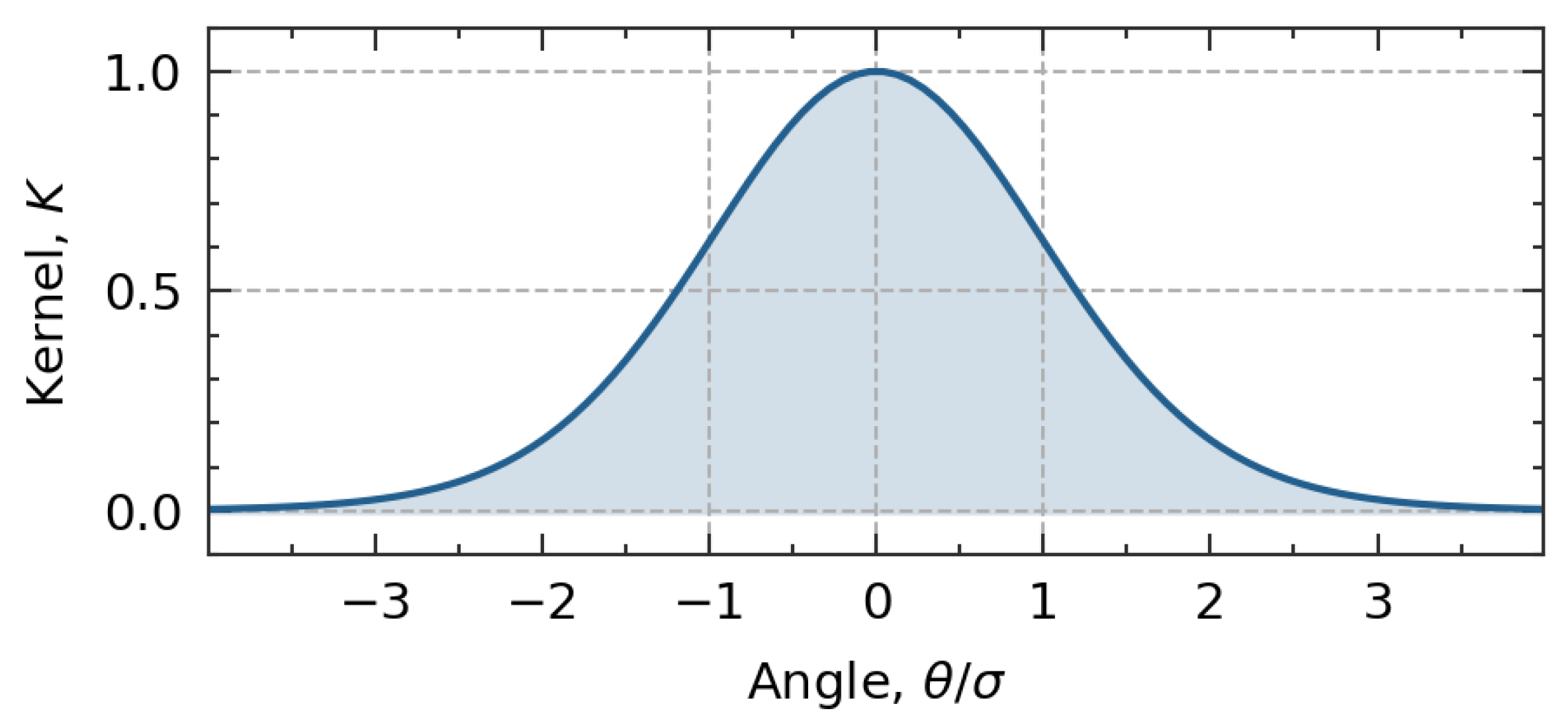
In the general methodology, the choice of kernel function is not strictly defined [14]. It can be based on elastic properties of thin-plate splines, and there are even some justifications for spherical geometries [15]. However, a radial Gaussian distribution is usually a good choice, and it is the choice used in SunPATH. For unit vectors on a spherical surface it can be written as

$$K_p\left(\mathbf{r}\right)=exp[({\mathbf{r}}_p·\mathbf{r}-1)/{\sigma }^2].$$

(8)

It can be checked that for small angles $\theta$ between $\mathbf{r}$ and ${\mathbf{r}}_p$

$$K_p\left(\mathbf{r}\right)\approx exp[-{\theta }^2/\left(2{\sigma }^2\right)],$$

(9)

where $\sigma$ is a half-width of Gaussian distribution (Figure 4). The half-width is usually selected to be about 3 times larger than the distance between sampling points $\sigma =3\rho$.

If the function is known at the sampling points $f_p=f\left({\mathbf{r}}_p\right)$, the amplitudes $A_p$ can be found by solving the linear matrix equation

$$f_p={\sum }_q{K}_{pq}{A}_q,$$

(10)

where $K_{pq}=K_p\left({\mathbf{r}}_q\right)$. The solution can be written in terms of inverse matrix

$$A_p={\sum }_q{K}_{pq}^{-1}{f}_q.$$

(11)

Note that the kernel matrix is symmetric by definition $K_{pq}=exp[({\mathbf{r}}_p·{\mathbf{r}}_q-1)/{\sigma }^2]=K_{qp}$, and the same property holds for its inverse $K_{pq}^{-1}=K_{qp}^{-1}$. However, from numerical point of view, the accuracy of matrix inversion can be limited for large matrices, and it is better to solve Equation (10) directly by using a matrix decomposition.

2.2. Integration over Sun Path

The optical efficiency of the solar concentrating subsystem of a CST system or any other function $f\left(\mathbf{r}\right)$ which depends on the sun position can be interpolated according to Equation (7). As the sun position is a known function of time $\mathbf{r}\left(t\right)$, it is also possible to say that the dependence $f\left(t\right)$ is known. The computation of annual output for CST systems involves integrals of the following form:

$${\left\{fw\right\}}_{\mathrm{year}}={\int }_{\mathrm{year}}f\left(t\right)w\left(t\right)dt,$$

(12)

where the notation ${\left\{\right\}}_{\mathrm{year}}$ is used as a shorthand for annual integration, and $w\left(t\right)$ is a weight function. The Direct Normal Irradiance (DNI) is often used as a weight.

The substitution of interpolation (7) into the integral (12) gives

$${\left\{fw\right\}}_{\mathrm{year}}={\sum }_p{A}_p{\left\{K_{p}w\right\}}_{\mathrm{year}}.$$

(13)

The amplitudes can be replaced with Equation (11)

$${\left\{fw\right\}}_{\mathrm{year}}={\sum }_{pq}{K}_{pq}^{-1}{\left\{K_{p}w\right\}}_{\mathrm{year}}{f}_q,$$

(14)

which can be rewritten in a short form as

$${\left\{fw\right\}}_{\mathrm{year}}={\sum }_q{\tilde{w}}_q{f}_q,$$

(15)

where

$${\tilde{w}}_q={\sum }_p{K}_{pq}^{-1}{\left\{K_{p}w\right\}}_{\mathrm{year}}.$$

(16)

Formula (15) means that the annual integrals can be reduced to a weighted sum. The coefficients (16) can be precomputed, because they depend on the fixed overlap integrals between the weight function and interpolation kernels. For tabulated data $w\left(t_n\right)$ with a small time step $\Delta t$, the overlaps can be found as

$${\left\{K_{p}w\right\}}_{\mathrm{year}}={\sum }_n{K}_p\left[\mathbf{r}\left(t_n\right)\right]w\left(t_n\right)\Delta t.$$

(17)

The accuracy of trapezoidal integration depends on the time step. The TMY3 standard uses one-hour step by default, which corresponds to the angular resolution of ${360}^{\circ }/24={15}^{\circ }$. This is too big for the kernels in Equation (17), and an interpolation is necessary to produce the data $w\left(t_n\right)$ with a smaller step. Usually, one-minute step is acceptable. Note that for some quantities like irradiance, which is a derivative of insolation, it is better to interpolate the insolation directly, as it is a monotonic function, and there are special algorithms for monotonic interpolation [16]. This ensures that the total annual insolation is unchanged and that the irradiance is always positive. Furthermore, note that the accuracy of the sum (17) can degrade for large number of terms because of the truncation errors. The errors can be minimized with the Kahan summation algorithm [17], which is used in SunPATH.

The calculation of annual averages is closely related to the annual integration. The annual average of a function $f\left(t\right)$ with the weight $w\left(t\right)$ is defined as

$${〈f,w〉}_{\mathrm{year}}=\frac{{\int }_{\mathrm{year}}f\left(t\right)w\left(t\right)dt}{{\int }_{\mathrm{year}}w\left(t\right)dt},$$

(18)

which can be rewritten in a shorter form by using the notation of Equation (12)

$${〈f,w〉}_{\mathrm{year}}=\frac{{\left\{fw\right\}}_{\mathrm{year}}}{{\left\{w\right\}}_{\mathrm{year}}}.$$

(19)

The substitution of Equation (15) gives the following formula for computing the annual average:

$${〈f,w〉}_{\mathrm{year}}=\frac{{\sum }_p{\tilde{w}}_p{f}_p}{{\sum }_p{\tilde{w}}_p}.$$

(20)

3. Test Case to Explore the Impact of Temporal and Spatial Resolutions

To explore the effectiveness of SunPATH in minimizing the number of sun position points one needs to simulate to accurately calculate the annual energy yield of the LCC subsystem of a CST plant, a test case was developed. The main goals in developing the test case were to ensure the following:

• It is representative of many CST plant configurations of interest, i.e., one can be fairly confident that the validity of the conclusions obtained from analyzing the results apply to many real CST plant of interest.
• It can be easily replicated, i.e., it can be described easily to the degree of detail needed to be easily modeled and analyzed by others.

To achieve these goals, the following actions were carried out:

• A location was selected that is characteristic of the range of latitudes, climatic, and solar resource conditions where CST plants are located, and for which real high-quality and high-temporal resolution solar Direct Normal Irradiance (DNI) datasets are readily available.
• Three consistent sets of solar DNI temporal series, at different temporal resolutions (1-min, 10-min, and 1-h), were selected that are also representative of the type of DNI temporal series on the selected location.
• A type of CST plant was selected which is representative of the type of CST plant that are currently being deployed commercially. This type of plant is a solar tower.
• A layout of the LCC system of the CST plant was selected, which is realistic, i.e., very similar in its optical behaviour to the LCC of commercial CST plants, but which can be easily specified, modeled, simulated, and analyzed.

For this test case, ray tracing simulations were performed, as described in Section 3.4, to compute the power delivered by the LCC subsystem at specific sun positions. Using these type of simulations, the annual energy delivered by the LCC subsystem was calculated in two completely different ways:

• In the temporal domain, carrying out a ray trace simulation once per instant of time and DNI value in the DNI temporal series being considered, to compute the power delivered by the LCC subsystem in each instant of time, and integrate the corresponding temporal power series.
• In the sun path spatial domain, running first SunPATH at different spacial sampling resolutions, to determine for each of those resolutions, the set of sun positions and associated weights with which to carry out ray tracing simulations and obtain the annual energy by direct summation of the results obtained from the simulations as described in Section 2.

Due to the very large number of computations needed to estimate the annual energy delivered by the LCC subsystem in the temporal domain approach, this approach was implemented on the High-Performance Facility (HPC) of The Cyprus Institute (CyI). Details of the implementation on the HPC are discussed in Section 4.

The overall scientific workflow that was followed is visualized in Figure 5. Within the sections that follow, details are given regarding each step of the workflow.

3.1. CST Plant Location

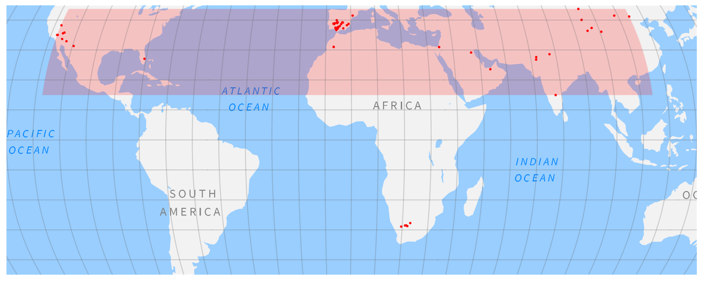
According to the CSP.guru database [18], of the 93 operational CST power plants in the world, totaling a nominal capacity of 6.2 GW, 87 of them, totaling 5.7 GW (92% of world’s total nominal capacity), are in the north hemisphere, with their North Latitudes in the interval $[14.{949}^{\circ },43.{76}^{\circ }]$, their East Longitudes in the interval $[-117.{559}^{\circ },114.{573}^{\circ }]$, and their “center of mass” at $36.{4377}^{\circ }$ North Latitude and $-3.{6454}^{\circ }$ East Longitude. Figure 6 shows the location of these plants and the window of latitudes and longitudes in which the plants in the northern hemisphere are located.

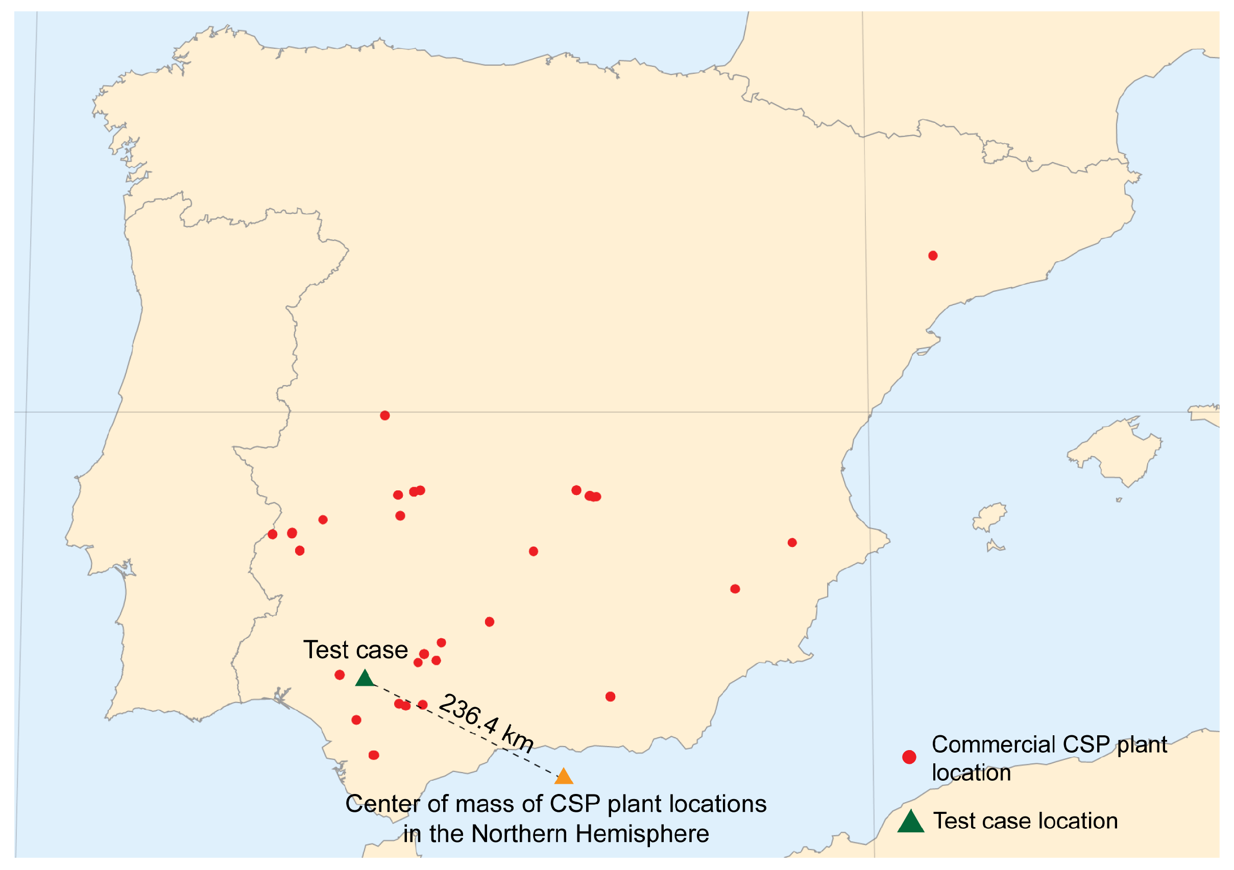
The selected plant location for the base case at $37.{4117}^{\circ }$ North Latitude and $-6.{00583}^{\circ }$ East Longitude, in the province of Seville (Spain) is quite close (236 km away) to the “center of mass” of all CST power plant locations in the northern hemisphere (see Figure 7). Thus, it is representative of the locations of these type of plants.

The province of Seville is home to 11 of the 50 commercial Spanish CST power plants, including the first three solar towers operating in the world. The neighboring provinces of Cordoba, Badajoz, and Cadiz, with similar climatic characteristics, accommodate 20 additional CST power plants. All these facts make this location a good example for the purposes of the analysis presented in this work. It is representative of the meteorological conditions of a good number of CST power plant projects, and, at the same time, its meteorological variability poses an interesting challenge to the optimization of the sampling procedure.

3.2. Solar DNI Time Series

For the test case, three different solar DNI time series have been considered. The difference between them is the time step: 1-min, 10-min, and 1-h. To ensure consistency among the time series, the 10-min and 1-h time series were built based on the 1-min solar DNI time series, with:

• Each element of the 1-min series being the average of the 12 5-s solar DNI readings in the given 1-min interval.
• Each element of the 10-min series being the average of the 10 1-min DNI values of the 1-min series in the given 10-min interval.
• Each element of the 1-h series being the average of the 60 1-min DNI values of the 1-min series in the given 10-min interval.
• The time-stamp of each point in each series being the time corresponding to the extreme of the corresponding interval.

Instead of using a Typical Meteorological Year, a real measured year was used. This year was selected as 2016. The selected measurement station was the meteorological station of the Group of Thermodynamics and Renewable Energy (GTER) of the University of Seville (https://gter.es/, (accessed on 4 June 2021). This measurement station measures solar DNI with a sampling and logging frequency of 0.2 Hz and an ISO first class Eppley NIP pyrheliometer mounted on a sun tracker Kipp and Zonen 2AP, with the location of the pyrheliometer being exactly the location considered for the base case, and discussed in the previous section.

Seville is located at an intermediate latitude and has a mild climate, with significant intra-annual and intra-daily variability, except during the summer months, as denoted by the significant number of partially cloudy days during the rest of the year [19], with monthly partially cloudy days between 5 (July) and 19 (December) in average for the period 2000–2012. The annual mean daily value of the DNI is approximately $5.7{\mathrm{kWh}/\mathrm{m}}^2$.

The year 2016 year has an annual DNI value of $2130.5\mathrm{kWh}/{\mathrm{m}}^2$, close to the average annual DNI value of the period 2002 to 2018 recorded at the GTER meteorological station ($2109.1\mathrm{kWh}/{\mathrm{m}}^2$). The 1-min solar DNI temporal series for the year 2016 used in this work has been subjected to the quality control procedures recommended by BSRN [20]. Only 1% of the whole data set did not pass all the BSRN recommended filters, mainly due to loss of synchronization of the clock of the data acquisition system with Internet time servers. Data with solar elevations lower than 0º have not been used in this study.

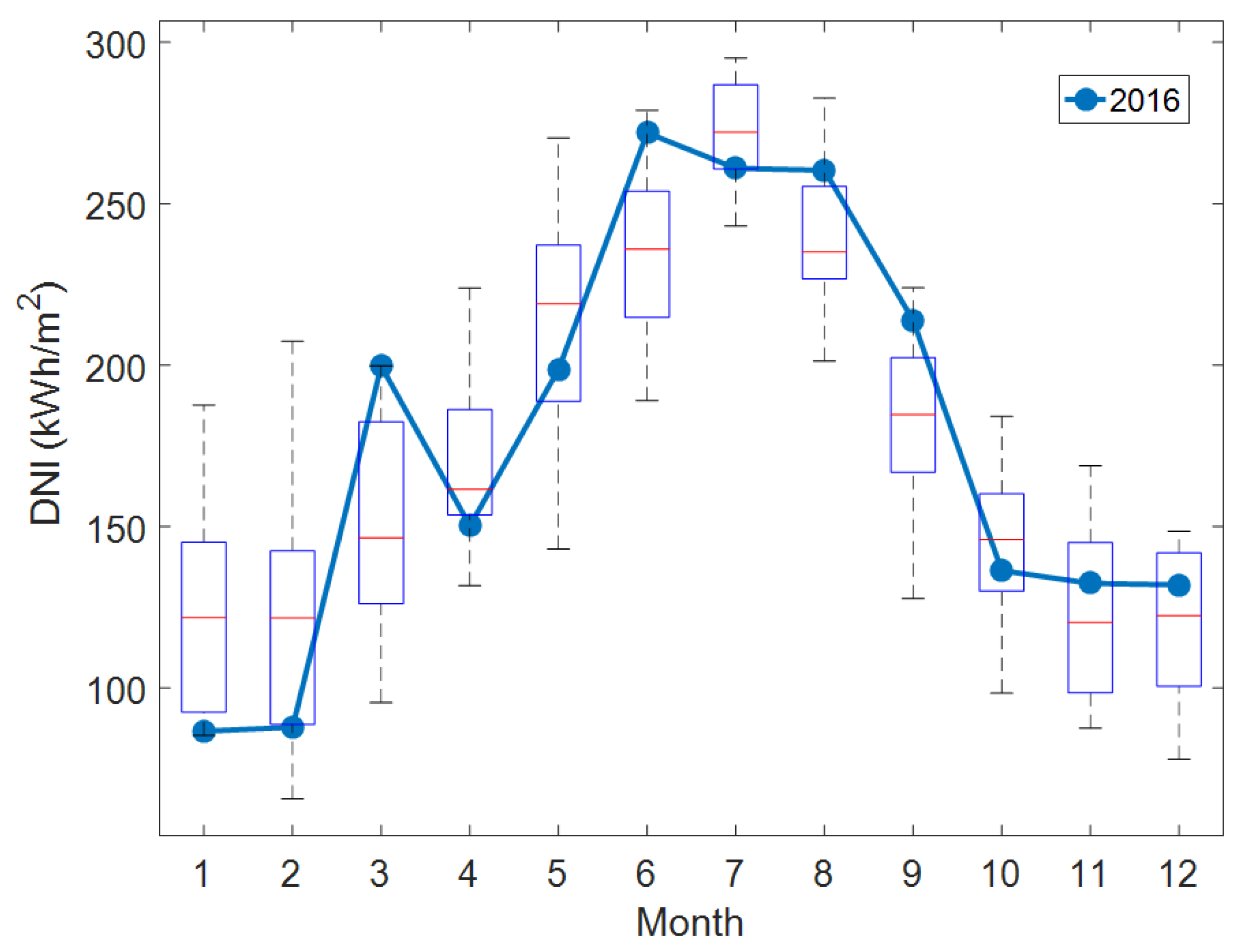
Figure 8 shows the observed monthly values for the year 2016 together with the observed monthly values of the entire available database (2002–2018) in a box-plot. Each box indicates the values comprised between the 25th (P25) and the 75th (P75) percentiles. Red horizontal lines indicate medians, and black horizontal lines represent the extreme observed values.

Note, however, that for this year the monthly cumulative values of March, June, August, and September are significantly high, while January, February, and April present low cumulative values.

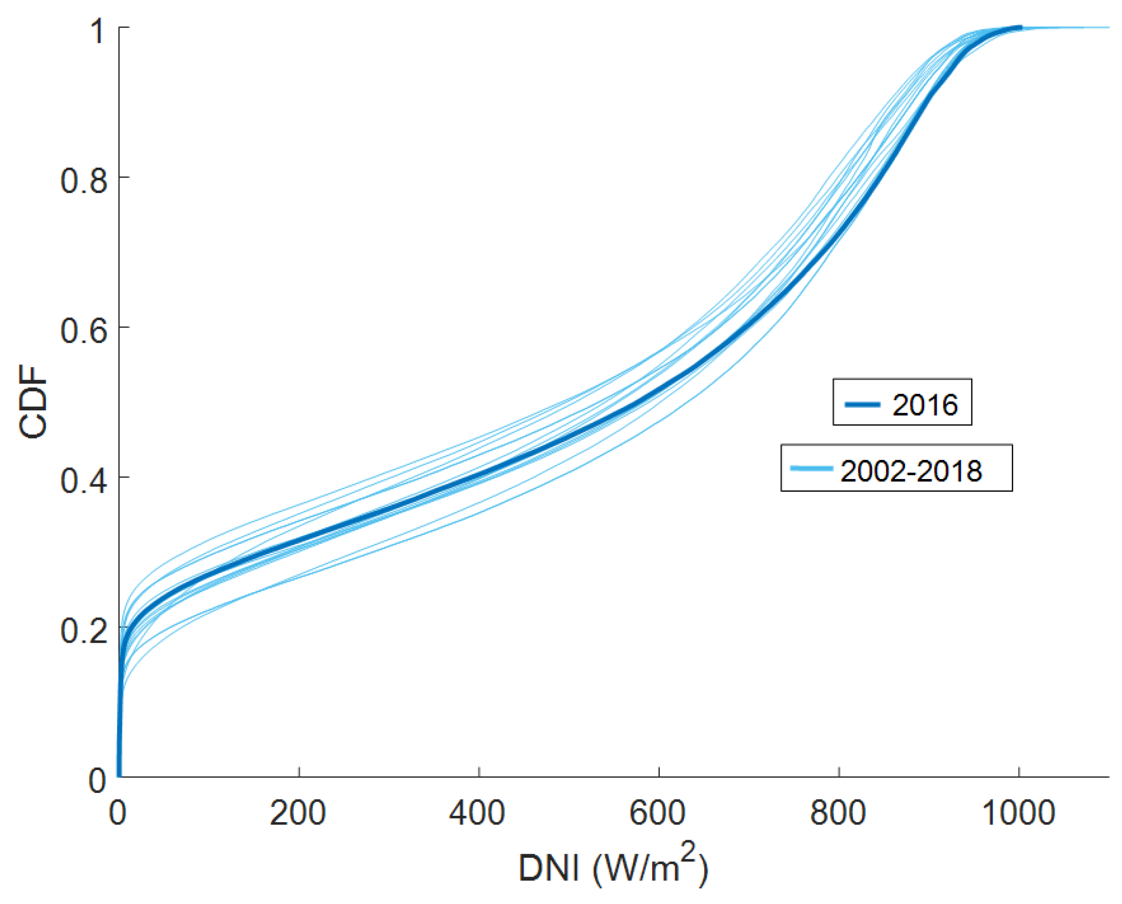
Figure 9 presents the cumulative distribution function (CDF) of the 1-min daylight DNI 2016 data together with CFDs of the rest of the years in the database. It clearly shows that the 1-min solar DNI temporal series for the year 2016 presents a CDF near the average of the entire database. It also shows that, in general, for the selected location, 50% of daylight data is equal or greater than around $575\mathrm{W}/{\mathrm{m}}^2$. 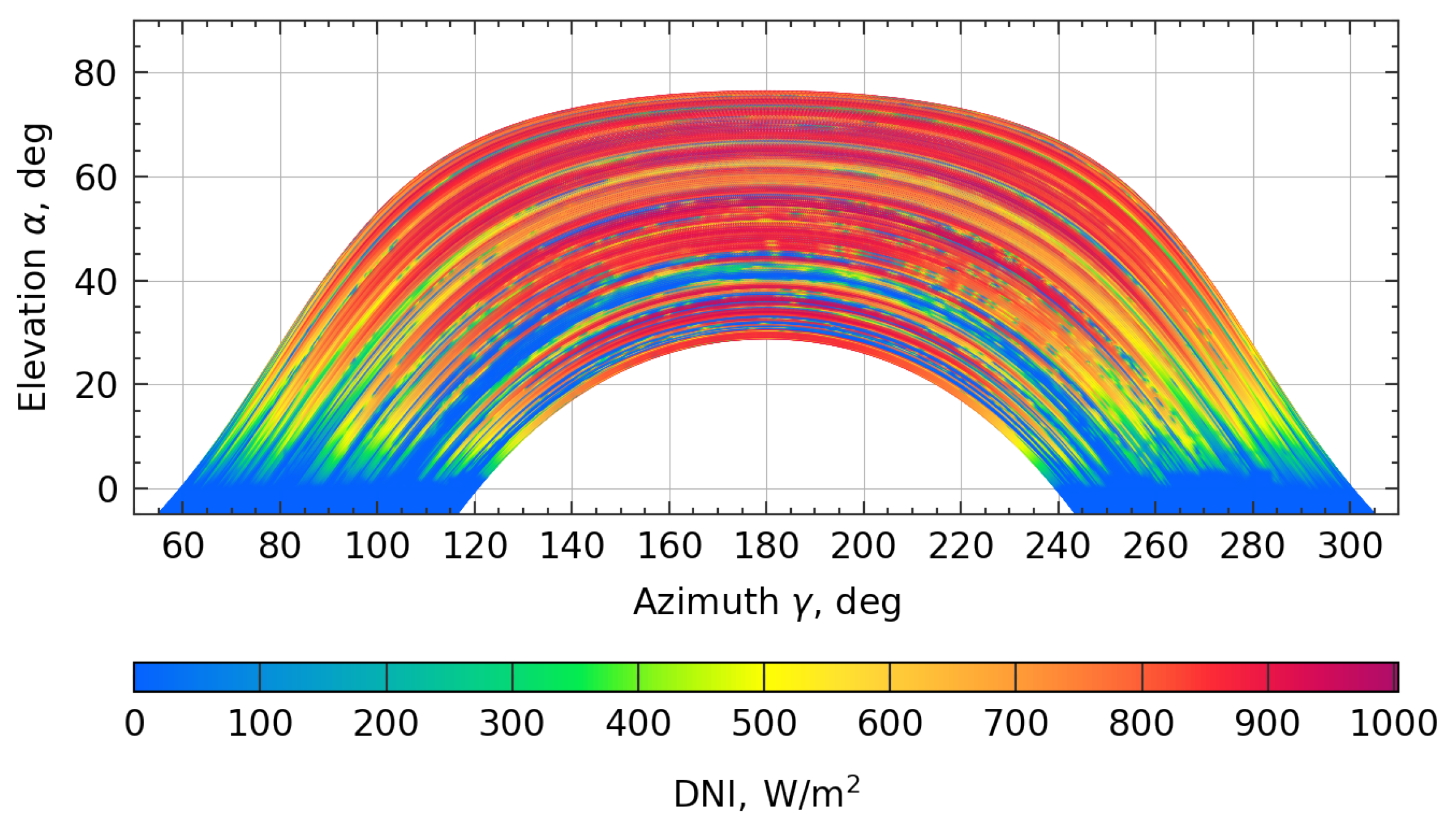The actual 1-min temporal data set is shown in Figure 10, in which a scatter plot of the simulation points, i.e., azimuth-elevation set, along with their corresponding DNI values is plotted.

3.3. Heliostat Field Layout

The heliostat field of the solar tower system considered in the case study is very similar to the PS10-like biomimetic heliostat field discussed by Noon et al. [2]. It is based upon the exactly same Fermat’s spiral phyllotaxis pattern, which is described by the following equations:

$$\begin{array}{c}{\theta }_k=2\pi {\phi }^{-2}k\end{array}$$

(21)

$$\begin{array}{c}{r}_k=a{k}^b\end{array}$$

(22)

where $(r_k,{\theta }_k)$ are the polar coordinates of heliostat k; $\phi =(1+\sqrt{5})/2$, is the golden ratio; and a and b are two constant coefficients, which are equal to 4.5 and 0.65, respectively.

Using the above equations, the layout of the heliostat field for the case study was obtained by:

• Considering:

  -

  The case study location as the location of the heliostat field.

  -

  The aiming point of all heliostats placed at the coordinates (0, 0, 121).

  -

  The number of heliostats in the heliostat field equal to 624, which is the actual number of heliostats of the PS10 solar tower.

• Allowing the heliostat position index k to vary from 1 to 3120, i.e., up to five times the number of heliostats established for the heliostat field.
• Eliminating all positions that have an y-coordinate either negative or positive but less than 25 m.
• Estimating for each one of the remaining 1479 heliostat positions an upper-limit of the annual weighted optical efficiency.
• Sorting the 1479 heliostat positions by the mentioned upper-limit from best to worst and selecting the first 624 positions.

For each heliostat position of interest, the upper-limit of the weighted optical efficiency, ${\eta }_k$, was estimated in the following way:

$${\eta }_k=\frac{{\int }_{year}{I}_b\left(t\right){\eta }_{cos,k}\left(t\right){\eta }_{\tau ,k}\left(t\right)dt}{{\int }_{year}{I}_b\left(t\right)dt}$$

(23)

In the above equation, $I_b$ is the solar DNI or “beam” irradiance for the test case location; ${\eta }_{cos,k}$ is the cosine factor for the given heliostat position k, i.e., the cosine of the angle between the normal to the heliostat and the unit vector in the direction of the sun; and ${\eta }_{t,k}\left(t\right)$ is the transmittance factor.

$I_{b,cd}$ is estimated using the 1977 ASHRAE solar DNI clear sky model [21] shown below. In this model, $s_z\left(t\right)$ is the vertical component of the unit vector in the direction of the sun, $I_0$ is the apparent extraterrestrial irradiance, and $\beta$ is atmospheric extinction coefficient. $I_0$ and $\beta$ are two location specific parameters, which are set equal to $1110\mathrm{W}/{\mathrm{m}}^2$ and 0.11, respectively, for the case study.

$$I_b\left(t\right)=I_0{e}^{-\beta /s_z\left(t\right)}$$

(24)

${\eta }_{\tau ,k}$ is estimated using the Sengupta and Wagner atmospheric attenuation model [22] shown below, with $\beta$ equal to 0.11 and where, d, is the slant range or distance in meters from the heliostat position k to the aiming point at the receiver.

$${\eta }_{\tau ,k}\left(t\right)=e^{-(1.0696\times {10}^{-5}+9.196\times {10}^{-4}\beta )d}$$

(25)

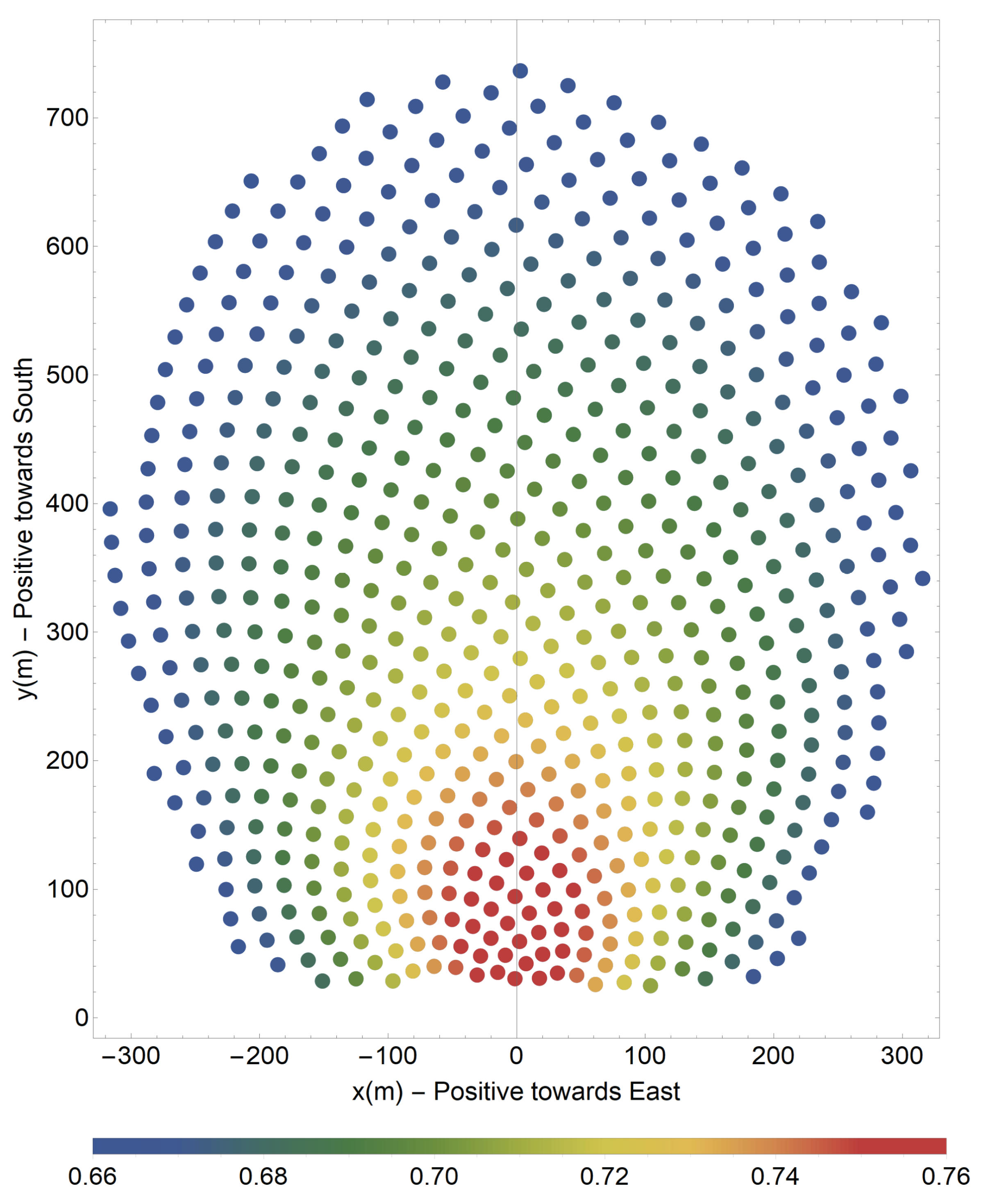
Figure 11 shows the final layout of the 624 heliostats of the heliostat field used for the test case, colored according to the values of their upper-limit of the the weighted optical efficiency.

The expression of the upper-limit of the weighted optical efficiency, as estimated for the test case:

• Does not consider shadowing and blocking effects,
• Considers a very simple model of the DNI variation along the day and the year and not real measurements,
• Considers also a relatively simple, optimistic and static model of the transmittance factor.

These simplifications greatly facilitate the computation of the upper-limits for any position on the field, while still providing a reasonable way to rank the suitability of any position to be part of the actual layout of the heliostat field and of obtaining a sensible heliostat field for the case study, which can be easily reproduce by anyone interested.

3.4. Tonatiuh++ Model

After generating the layout of the PS10-like biomimetic heliostat field, the entire field, the tower, and the receiver were then modeled within Tonatiuh++ using its scripting capabilities. The goal was to model the main features of the heliostat field and tower as close as possible to the actual features of the original PS10 plant as discussed in [2]. It is worth mentioning here that Tonatiuh++ is essentially the evolution of Tonatiuh [23], the de facto standard of open source Monte Carlo ray tracers for the modeling of solar concentrating systems [24]. Tonatiuh++ is currently being developed by The Cyprus Institute (CyI), and its development aims to provide a ray tracing tool with enhanced functionalities and advanced features, to be much faster, easier to use, and more flexible than is predecessor. Tonatiuh++ will be an open access tool that will be available within the year.

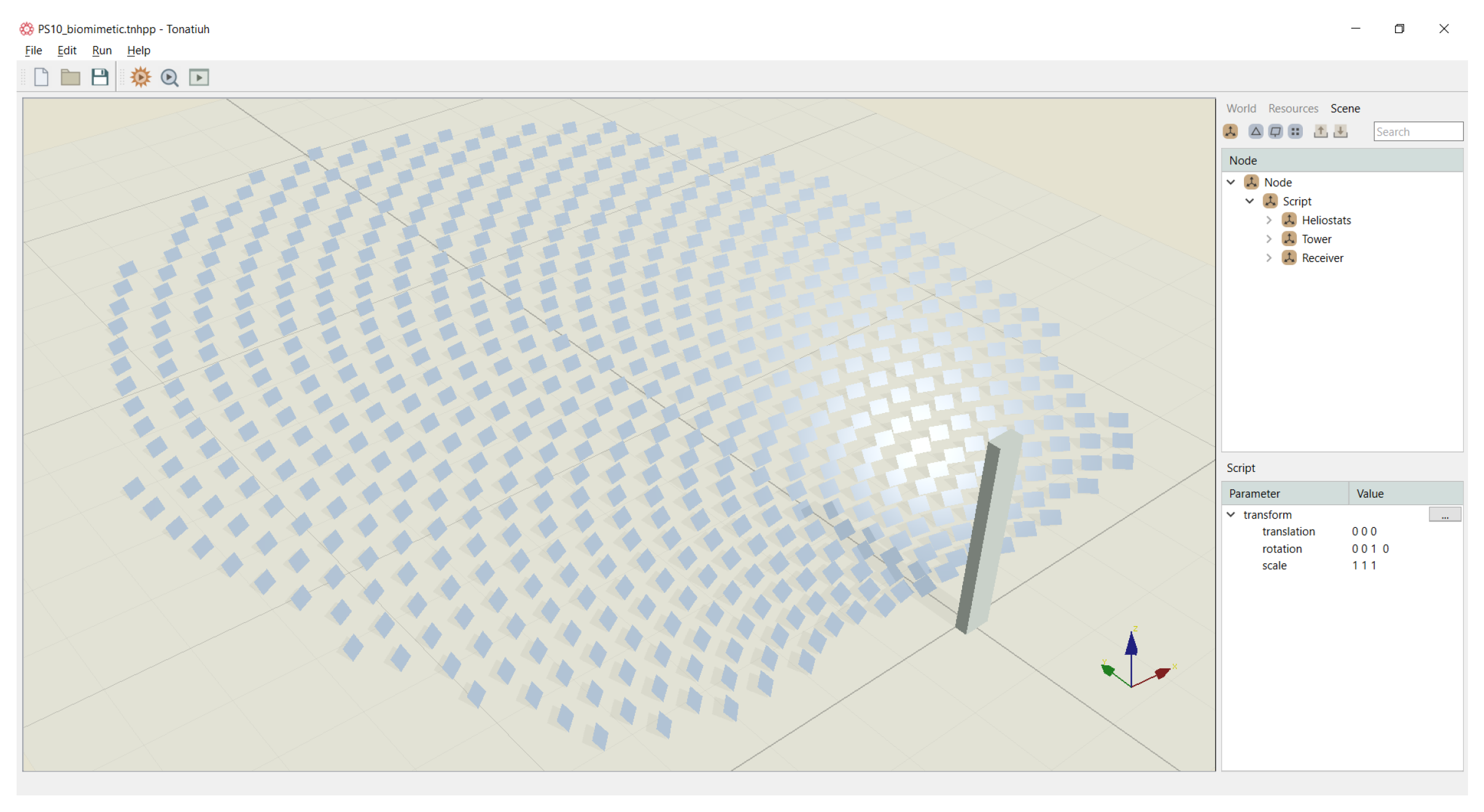
Figure 12 shows a screenshot of the solar concentrating field as generated in Tonatiuh++. Given the global (X, Y, Z) coordinate system of Tonatiuh++, the origin of the tower was placed at (0, 0, 0), with the positive X axis direction oriented towards the East, the positive Y direction oriented towards the North and the positive Z axis oriented towards the Zenith. The body shape of the tower was designed on the basis of the actual PS10 tower, with a frontal view of 18 m, a lateral view of 8 m and a height of 115 m. A rectangular flat target/receiver of 12 m in height and 13.78 m in width is accommodated on top of the tower with an appropriate tilting angle leaning towards the heliostat field.

As indicated in

Table 1. Main characteristics of the PS10-like biomimetic heliostat field modeled in Tonatiuh++.

Location
Longitude	37${}^{\circ }$24${}^{\prime }$42${}^{″}$ North
Latitude	6${}^{\circ }$0${}^{\prime }$21${}^{″}$ West
Heliostat Field
No. of Heliostats	624
Width	12.84 m
Height	9.45 m
Reflectivity	0.88
${\sigma }_{opt}$	2 mrad
Tracking	Azimuth-Elevation
Tower and Receiver
Tower height	115 m
Receiver type	Rectangular billboard
Receiver width	13.78 m
Receiver height	12 m
Aiming point	(0.0, 0.0, 121.0) m
Receiver normal direction vector	(0.0, 0.9763, −0.2165) m

, the heliostat field counts 624 heliostats, each with a single facet parabolic rectangular mirror of 12.84 m in width and 9.45 m in height, thus yielding approximately 75,715 ${\mathrm{m}}^2$ of total reflective area. All heliostats were set to aim at the center point of the receiver, i.e., at (0, 0, 121) m. The focal length of each heliostat was automatically calculated as the distance measured from the center of the mirror of each heliostat to the aim point on the receiver. An azimuth-elevation system was considered for the tracking system of the heliostats, while the reflectivity of the mirrors was set to 0.88 with a Gaussian distribution slope error of 2 mrad.

In the details of the ray tracing simulations, the Buie sunshape [25] was used with a circumsolar ratio of $2\%$.

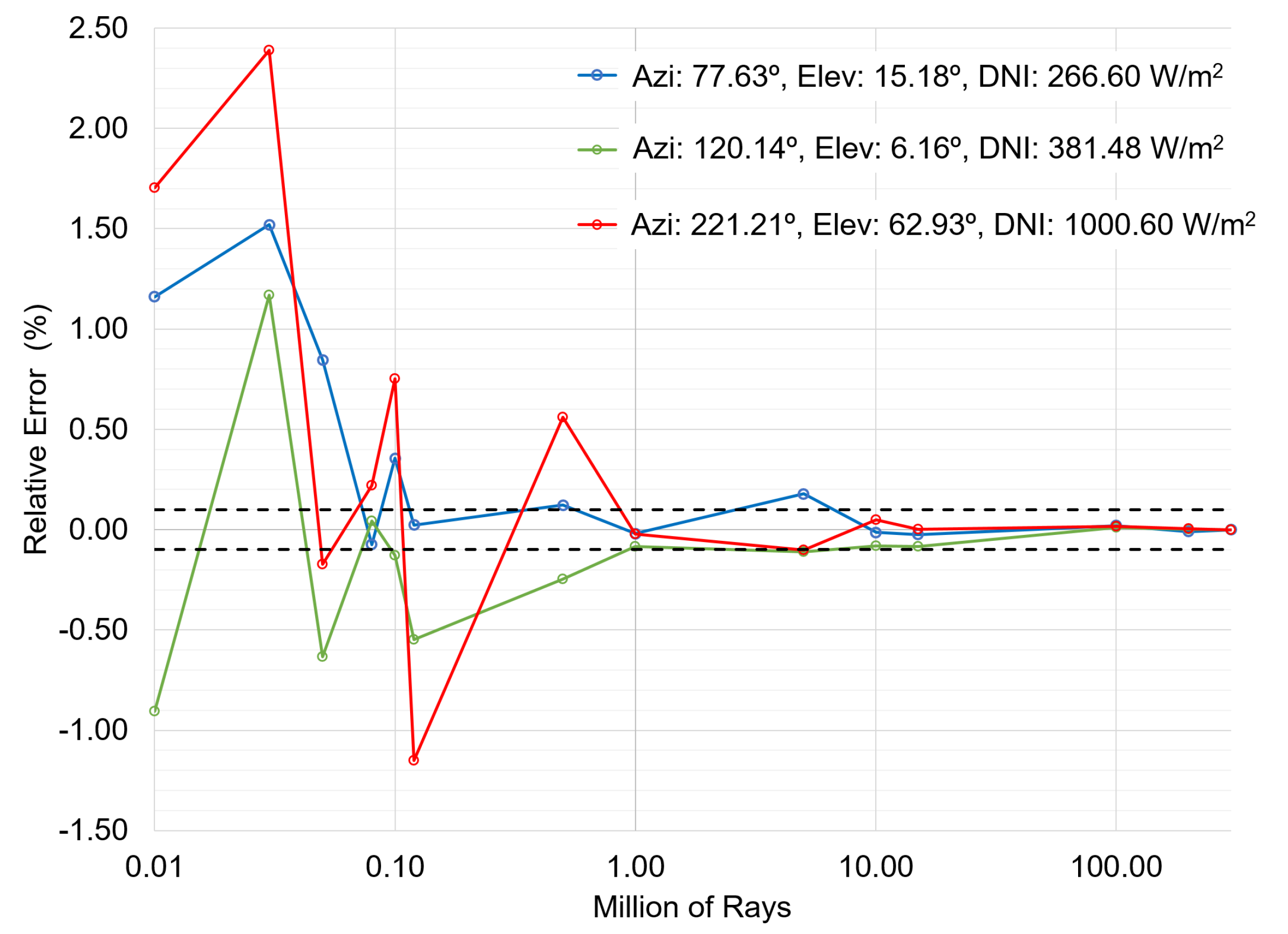
In order to establish the minimum number of rays to cast in each simulations, a ray convergence study was carried out for three different tuples of sun position and DNI values. For each tuple (sun position, DNI value), the ground truth was considered to be the result obtained casting in Tonatiuh++ 300 million rays. Figure 13 shows how the relative error with respect to the ground truth varies for each of the three tuples as a function of the number of rays cast. As the figure shows, a minimum of 10 million rays needs to be cast to reach relative errors with respect to the ground truth that are less than $\pm 0.1\%$. For this reason, all Tonatiuh++ simulations to estimate the annual energy delivered by the LCC subsystem were carried out casting 15 million rays.

3.5. Sun Positions

The compute position of the sun in terms of azimuth and zenith angle for given instances of times during the year is needed both in SunPATH and in Tonatiuh++. These two programs can use several algorithms to compute the sun position, and can also read the sun positions provided by third-party applications.

The default algorithm used in SunPATH and Tonatiuh is the PSA+ algorithm [13], which is an updated version of the PSA algorithm [26]. Both the PSA+ and original PSA algorithm have a very small computational footprint, can be used in a large variety of computer systems and controllers, and are fast. For the period 2020 to 2050, the maximum error in azimuth of the PSA+ with respect to the sun position as provided by the Multiyear Interactive Computer Almanac (MICA) of the U.S Naval Observatory is less than 107 arcseconds, with a mean deviation of 10.61 arcseconds, and the maximum error in zenith angle is less than 27.8 arcseconds, with a mean deviation of 7.28 arcseconds.

To test if these type of errors in the angular position of the sun could have any impact on the estimates of the annual energy delivered by the LCC subystem of a CST system in either of the two approaches being considered, in both approaches the energy estimates were carried out using both the sun positions provided by MICA and the the sun positions provided by the PSA+ algorithm. As no significant differences were identified, it was concluded that using the PSA+ algorithm in SunPATH and in Tonatiuh++ is more than appropriate for the purpose of estimating annual characteristics of CST systems, which depend on the sun position.

4. Energy Estimates on the Temporal Domain

Ray tracing calculations are computationally expensive with the computational time required scaling with the number of rays to cast for each one of the simulation. Running directly on the temporal domain would require massive computational effort, especially for the 1 min data set. For this reason, a High-Performance Computing (HPC) implementation of Tonatiuh++ has been developed in order to make this kind of calculations feasible.

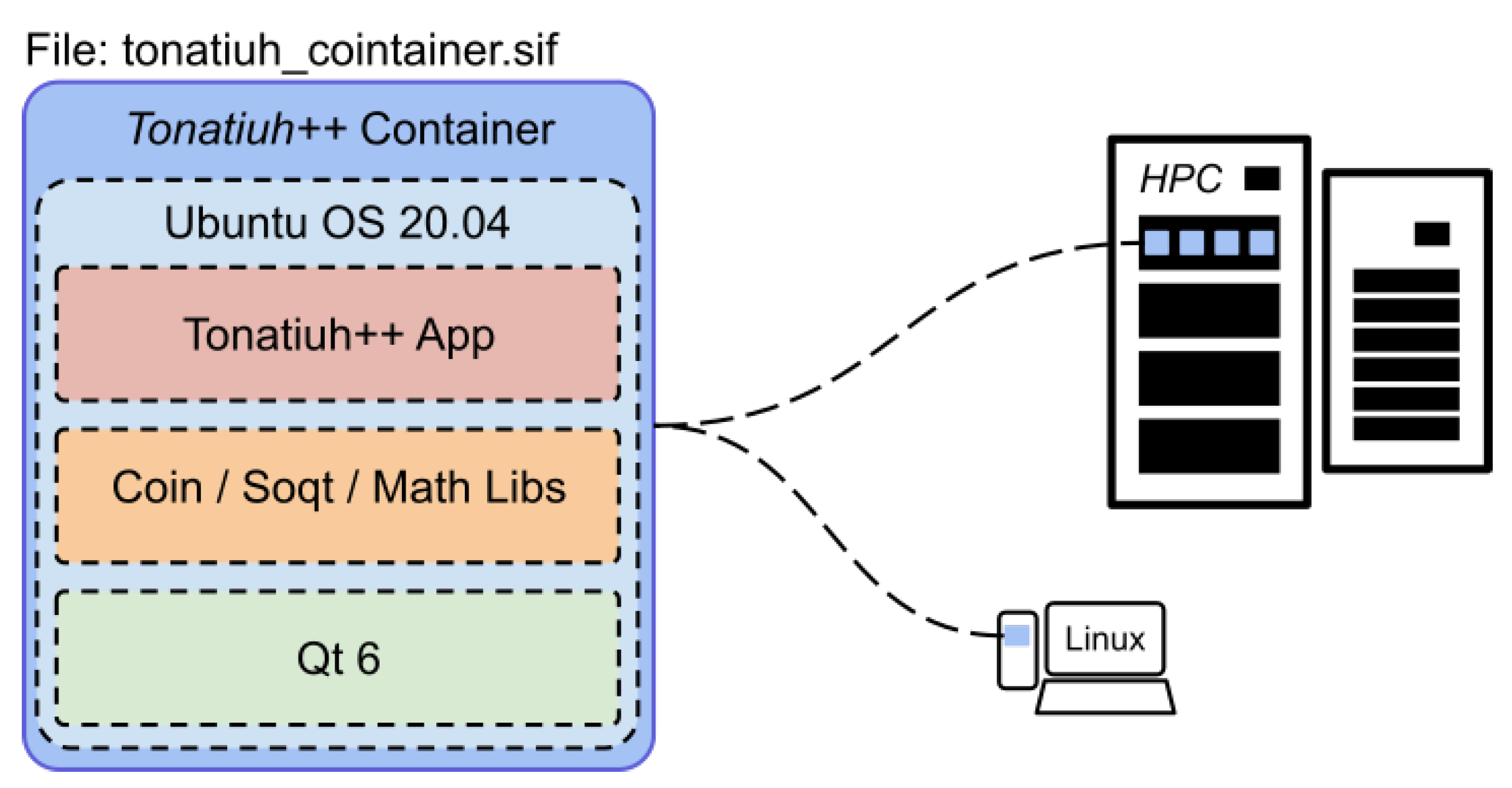
Tonatiuh++ is a cross-platform application, and running it on a High-Performance Computer (HPC) did not require extensive platform porting. Furthermore, the portability of the system has been improved by (i) automating invocations of the executable via scripts and the command-line, and (ii) building a singe-file, Singularity-based container that includes all dependencies and allows Tonatiuh++ to run on virtually any Linux or HPC system (Figure 14).

This approach greatly simplifies the experimentation process and strengthens reproducibility, as it requires not software installation on the target HPC systems. All that is needed is the "tonatiuh_container.sif" file and a system that supports the open-source Singularity software.

Tonatiuh++ is a multi-threaded application which yields very high speedups on high core-count systems. Additionally, due to the nature of the computation, it can be easily parallelized across different nodes through a time-based partitioning of the problem set. For the temporal domain runs, one of the HPC systems at the HPC Facility of the Cyprus Institute has been employed, that is based on AMD EPYC™, and which has 128 physical cores per node. At any given time up to 8 nodes could be used. The combination of the above allowed the 1 min annual simulation (254,871 day-time minutes and casting 15 million rays per data-point) to be performed in under 24 h on 1024 cores on the HPC system. In contrast, running this on a fast workstation would take approximately 48 times longer (i.e., 1–2 months).

5. Energy Estimates on the Spatial Domain Using SunPATH

SunPATH requires 1-min irradiance data for an accurate integration. However, it can also accept 10-min or 1-h data. In these cases, a linear monotonic interpolation of insolation is applied to generate 1-min irradiance data.

The main inputs for SunPATH are the latitude of the location and the desired spatial resolution of the sky. As an output, it produces a set of sun positions (azimuth and elevation). These positions can be used to sample the optical efficiency of the LCC subsystem of a CST system using an optical modeling tool, such as a ray tracer. The sampled values are necessary for SunPATH to build an interpolated function. If the irradiance data are supplied, SunPATH can compute the integration weights of the sun nodes and perform the annual integration.

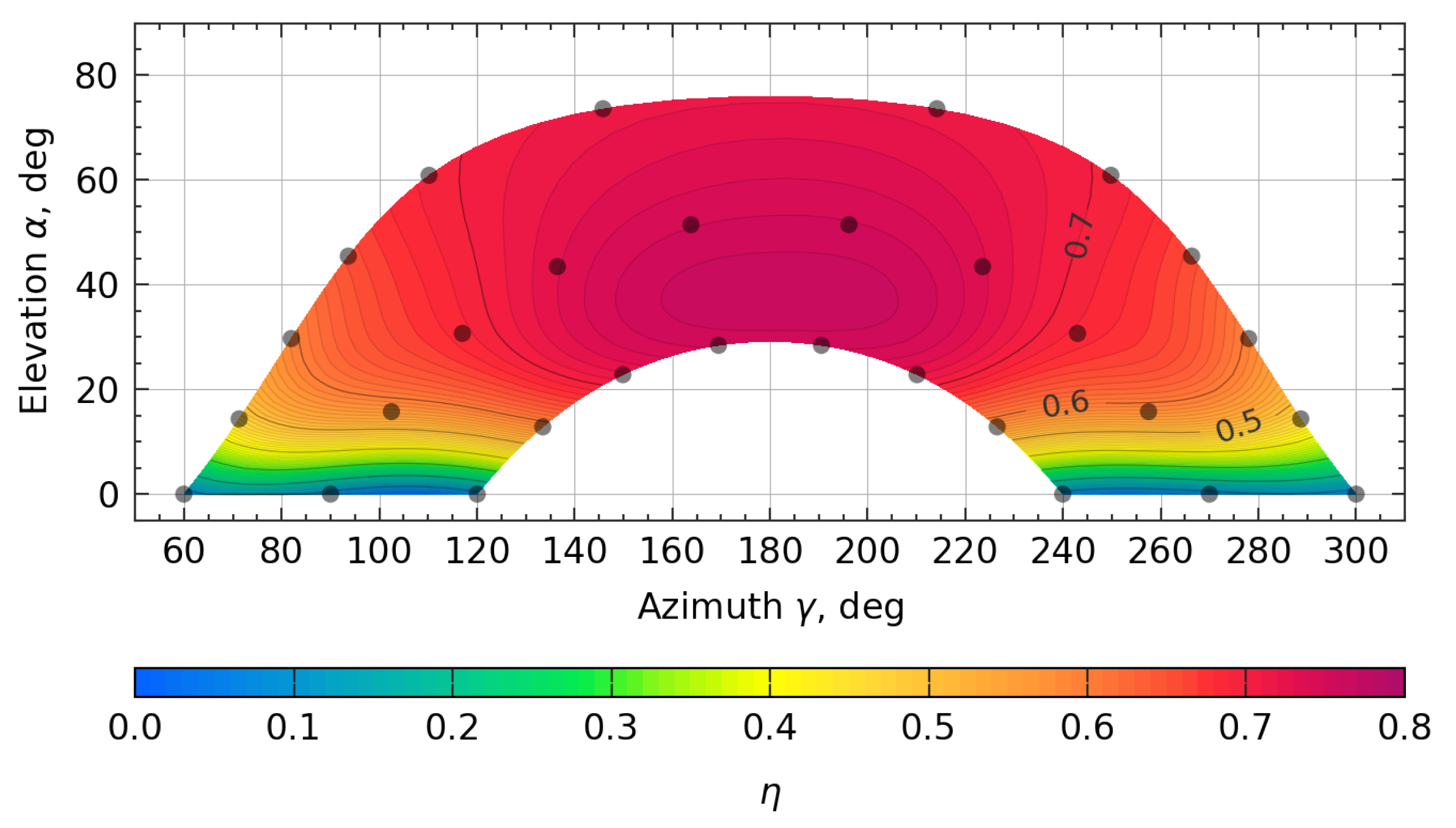
For the test case, SunPATH was run at three different sampling levels—30, 52, and 114 sampling points, which correspond to a 20, 15, and 10 degree resolution of the partitioning of the spherical region in the celestial sphere containing the sun path. Figure 15 illustrates an example of the interpolated optical efficiency using SunPATH as obtained for the 30 sampling point level and a 20 degree resolution.

6. Comparison of Results

The results of the exploration in the time domain indicate that, at least to estimate annual integrals, 1-h data is enough to estimate the integrals with high accuracy (~0.2% of error for trapezoidal integration and 0.02% for integration with interpolation of second order) (

Table 2. Comparison of the annual energy in GWh intercepted between the temporal and spatial domain simulations.

Time Step	Temporal Domain		Spatial Domain (SunPATH)
	Trapezoidal Rule	Second Order Interpolation	30 pts	52 pts	114 pts
1 min	107.831	107.831	107.781	107.745	107.800
10 min	107.824	107.827	107.784	107.747	107.802
60 min	107.603	107.807	107.926	107.863	107.908

and

Table 3. Relative error (%) of the calculated annual energy intersected with respect to the 1 min temporal data results obtained using the second order interpolation.

Time Step	Temporal Domain		Spatial Domain (SunPATH)
	Trapezoidal Rule	Second Order Interpolation	30 pts	52 pts	114 pts
1 min	0	0	−0.046	−0.080	−0.029
10 min	−0.006	−0.004	−0.046	−0.078	−0.027
60 min	−0.211	−0.022	0.088	0.030	0.071

). This accuracy is very remarkable taking into account that the optical efficiency of the LCC subsystem at any given instant can have variations about 0.05% if the convergence requires more rays. Note, however, that the deviations can lead to positive and negative contributions to the annual integral which compensate each other so that the actual result is more accurate.

For the same test case, the computations of these integrals in the spatial domain were also explored, using SunPATH in tandem with Tonatiuh++. The comparison between the time and spatial domain approaches clearly indicate that the spatial domain using SunPATH is dramatically more computationally efficient than the time domain approach.

7. Conclusions

Based upon the results presented and discussed in the previous section and, in general, on the work presented and discussed in this article, the following conclusions can be drawn.

• Integrals that are of interest in the analysis, design, and optimization of CST systems, such as the annual optical efficiency of the LCC subsystem, can be accurately computed or estimated in two distinct ways: on the time domain and on the spatial domain.
• For the CST test case presented in this article, which is highly representative of the commercial CST systems being deployed worldwide, the computation of these integrals in the time domain was explored using 1-min, 10-min, and 1-h solar DNI input data and using CyI’s HPC and an open-source ray tracer, Tonatiuh++, that is being actively developed at CyI.
• The results of the exploration in the time domain indicate that, at least to estimate annual integrals, 1-h data is enough to estimate the integrals with high accuracy (less than 0.2% of error) as long as the optical efficiency of the LCC subsystem at any given instant is estimated with an accuracy better than 0.1%.
• For the same test case, the computations of these integrals in the spatial domain were also explored, using SunPATH, another open source software tool being actively developed at CyI, in tandem with Tonatiuh++.
• The results of the exploration in the spatial domain indicate that, for any of the three sets of DNI data provided to SunPATH (1-min, 10-min, and 1-h) the number of sun positions and weights that have to be requested from SunPATH and used in Tonatiuh++ to accurately compute the annual integrals of interest could be as low as 30 if the heliostat field is not symmetric with respect to the N-S line, and as low as 15 if it is symmetric.
• The comparison between the time and spatial domain approaches clearly indicate that the spatial domain using SunPATH is dramatically more computationally efficient than the time domain approach.
• The fact that the results of the annual integral estimates in the temporal and spatial domains do not change at all when computing the sun positions using MICA or using the PSA+ algorithm show that using the PSA+ algorithm allows to accurately estimate the annual integrals.
• In summary, for the test case considered in this article, it has been shown that to compute the annual energy delivered by the LCC subsystem with a relative error less than 0.1% it is enough to do the following.
  • Provide SunPATH with 1-h DNI data as input, using the PSA+ algorithm to compute the associated sun positions.
  • Request from SunPATH the sun position and weights of just 30 points in the celestial sphere.
  • Run Tonatiuh++ to simulate these 30 points using 15 million rays per run.
• As the test case is highly representative, it is expected that a similar use of the PSA+ sun position algorithm, SunPATH and Tonatiuh++ for other CST systems will deliver similar results.

8. Future Work

Although the proposed approach shows an excellent accuracy in the calculation of annual integrals, it should be realized that the difference between the interpolated and reference function can be large. The integration can be considered as an averaging of positive and negative deviations, which can cancel each other and lead to a good accuracy. It would be interesting in this regard to investigate how to minimize the RMS accuracy of interpolation.

Note that the proposed approach for interpolation can be sensitive to the choice of half-widths for the spherical Gaussian kernels. This is a common issue in the theory of meshless interpolation with radial basis functions, and there are many options how to choose the shape parameters of the kernels. As an interesting alternative, the interpolation with thin-plate splines can be considered, which does not require any shape parameters.

References

- Li, C.; Zhai, R.; Yang, Y. Optimization of a Heliostat Field Layout on Annual Basis Using a Hybrid Algorithm Combining Particle Swarm Optimization Algorithm and Genetic Algorithm. Energies 2017, 10, 1924. [Google Scholar] [CrossRef] [Green Version]
- Noone, C.J.; Torrilhon, M.; Mitsos, A. Heliostat field optimization: A new computationally efficient model and biomimetic layout. Sol. Energy 2012, 86, 792–803. [Google Scholar] [CrossRef]
- Reinholz, A.; Husenbeth, C.; Schwarzbözl, P.; Buck, R. Optimizing heliostat positions with local search metaheuristics using a ray tracing optical model. AIP Conf. Proc. 2017, 1850, 160023. [Google Scholar] [CrossRef]
- Collado, F.J.; Guallar, J. Quick design of regular heliostat fields for commercial solar tower power plants. Energy 2019, 178, 115–125. [Google Scholar] [CrossRef]
- Wagner, M.J.; Wendelin, T. SolarPILOT: A power tower solar field layout and characterization tool. Sol. Energy 2018, 171, 185–196. [Google Scholar] [CrossRef]
- Grigoriev, V.; Corsi, C.; Blanco, M. Fourier sampling of sun path for applications in solar energy. AIP Conf. Proc. 2016, 1734, 20008. [Google Scholar] [CrossRef] [Green Version]
- Chen, C.J. Physics of Solar Energy, 1st ed.; Wiley: Hoboken, NJ, USA, 2011. [Google Scholar]
- Späth, H. Two Dimensional Spline Interpolation Algorithms; CRC Press: Boca Raton, FL, USA, 1993. [Google Scholar]
- Richter, P.; Tinnes, J.; Aldenhoff, L. Accurate interpolation methods for the annual simulation of solar central receiver systems using celestial coordinate system. Sol. Energy 2021, 213, 328–338. [Google Scholar] [CrossRef]
- Scipy. SciPy—SciPy v1.6.1 Reference Guide. SciPy.org, 2021. Available online: https://scipy.org/ (accessed on 4 June 2021).
- Schöttl, P.; Ordóñez Moreno, K.; van Rooyen, D.W.; Bern, G.; Nitz, P. Novel sky discretization method for optical annual assessment of solar tower plants. Sol. Energy 2016, 138, 36–46. [Google Scholar] [CrossRef]
- Binotti, M.; Manzolini, G.; Zhu, G. An alternative methodology to treat solar radiation data for the optical efficiency estimate of different types of collectors. Sol. Energy 2014, 110, 807–817. [Google Scholar] [CrossRef]
- Blanco, M.J.; Milidonis, K.; Bonanos, A.M. Updating the PSA sun position algorithm. Sol. Energy 2020, 212, 339–341. [Google Scholar] [CrossRef]
- Li, H.; Mulay, S.S. Meshless Methods and Their Numerical Properties; CRC Press: Boca Raton, FL, USA, 2013. [Google Scholar]
- Wessel, P.; Becker, J.M. Interpolation using a generalized Green’s function for a spherical surface spline in tension. Geophys. J. Int. 2008, 174, 21–28. [Google Scholar] [CrossRef] [Green Version]
- Fritsch, F.N.; Carlson, R.E. Monotone Piecewise Cubic Interpolation. SIAM J. Numer. Anal. 1980, 17, 238–246. [Google Scholar] [CrossRef]
- Press, W.H. Numerical Recipes 3rd Edition, 3rd ed.; Cambridge University Press: Cambridge, UK; New York, NY, USA, 2007. [Google Scholar]
- Lilliestam, J.; Thonig, R.; Zang, C.; Gilmanova, A. CSP.guru (Version 2021-01-01) [Data set]. 2021. Available online: https://zenodo.org/record/4613099#.YPjF-kARWUk (accessed on 4 June 2021). [CrossRef]
- Moreno-Tejera, S.; Silva-Pérez, M.A.; Lillo-Bravo, I.; Ramírez-Santigosa, L. Solar resource assessment in Seville, Spain. Statistical characterisation of solar radiation at different time resolutions. Sol. Energy 2016, 132, 430–441. [Google Scholar] [CrossRef]
- Mcarthur, L.J.B. World Climate Research Programme Baseline Surface Radiation Network (BSRN) Operations Manual Version 2.1; Technical Report WMO/TD-No.1274; World Meteorological Organization: Downsview, ON, Canada, 2005. [Google Scholar]
- Jordan, R.C.; Liu, B.Y.H. Applications of Solar Energy for Heating and Cooling of Buildings; American Society of Heating, Refrigerating and Air Conditioning Engineers, Inc.: New York, NY, USA, 1977; p. 206. [Google Scholar]
- Sengupta, M.; Wagner, M.J. Atmospheric attenuation in Central Receiver Systems from DNI measurements. In Proceedings of the World Renewable Energy Forum, WREF 2012, Including World Renewable Energy Congress XII and Colorado Renewable Energy Society (CRES) Annual Conference, Denver, Colorado, 13–17 May 2012; Volume 1, pp. 129–134. [Google Scholar]
- Blanco, M.J.; Amieva, J.M.; Mancillas, A. The Tonatiuh Software Development Project: An Open Source Approach to the Simulation of Solar Concentrating Systems. In Proceedings of the ASME 2005 International Mechanical Engineering Congress and Exposition, Orlando, FL, USA, 5–11 November 2005; ASME: Orlando, FL, USA, 2005; pp. 157–164. [Google Scholar] [CrossRef]
- Wang, Y.; Potter, D.; Asselineau, C.A.; Corsi, C.; Wagner, M.; Caliot, C.; Piaud, B.; Blanco, M.; Kim, J.S.; Pye, J. Verification of optical modelling of sunshape and surface slope error for concentrating solar power systems. Sol. Energy 2020, 195, 460–474. [Google Scholar] [CrossRef]
- Buie, D.; Monger, A.G.; Dey, C.J. Sunshape distributions for terrestrial solar simulations. Sol. Energy 2003, 74, 113–122. [Google Scholar] [CrossRef]
- Blanco-Muriel, M.; Alarcón-Padilla, D.C.; López-Moratalla, T.; Lara-Coira, M. Computing the solar vector. Sol. Energy 2001, 70, 431–441. [Google Scholar] [CrossRef]
Figure 1.
Relative time spent by the sun at different declinations.
Figure 2.
Relative (0 to 1) amount of time spent by the sun at different locations in the celestial sphere as function of hour angle and declination.
Figure 3.
Graphical User Interface (GUI) of the open source computer program SunPATH.
Figure 4.
Kernel function for radial Gaussian distribution (
8).
Figure 5.
Scientific workflow followed for performing the ray tracing simulations.
Figure 6.
Location of all commercial CST power plants currently in operation and the window of latitudes and longitudes in which the plants in the northern hemisphere are located.
Figure 7.
Test case location and its proximity to the center of mass of the location of the CST power plants currently in operation in the northern hemisphere.
Figure 8.
Monthly distribution of the DNI dataset for the location of Seville on the selected year (2016 in a blue line) and box-plot of the monthly cumulative values for the entire database (2002–2018).
Figure 9.
Cumulative distribution function of the 1-min DNI data for the location of Seville on the selected year (2016 in a blue line) and CDFs of the entire 1-min database (2002–2018).
Figure 10.
The 1-min temporal data set colored with the corresponding DNI value at each simulation point.
Figure 11.
Heliostat field layout used for the case study, colored according to the values of their upper-limit of the the weighted optical efficiency.
Figure 12.
The developed PS10-like biomimetic solar field within Tonatiuh++.
Figure 13.
Tonatiuh++ ray tracing convergence analysis.
Figure 14.
Tonatiuh++ container architecture.
Figure 15.
Interpolation of optical efficiency using SunPATH with 30 nodes.