Incentive-Based Demand Response Framework for Residential Applications: Design and Real-Life Demonstration

Abstract

In 2020, residential sector loads reached 25% of the overall electrical consumption in Europe and it is foreseen to stabilise at 29% by 2050. However, this relatively small increase demands, among others, changes in the energy consuming behaviour of households. To achieve this, Demand Response (DR) has been identified as a promising tool for unlocking the hidden flexibility potential of residential consumption. In this work, a holistic incentive-based DR framework aiming towards load shifting is proposed for residential applications. The proposed framework is characterised by several innovative features, mainly the formulation of the optimisation problem, which models user satisfaction and the economic operation of a distributed household portfolio, the customised load forecasting algorithm, which employs an adjusted Gradient Boosting Tree methodology with enhanced feature extraction and, finally, a disaggregation tool, which considers electrical features and time of use information. The DR framework is first validated through simulation to assess the business potential and is then deployed experimentally in real houses in Northern Greece. Results demonstrate that a mean 1.48% relative profit can be achieved via only load shifting of a maximum of three residential appliances, while the experimental application proves the effectiveness of the proposed algorithms in successfully managing the load curves of real houses with several residents. Correlations between market prices and the success of incentive-based load shifting DR programs show how wholesale pricing should be adjusted to ensure the viability of such DR schemes.

1. Introduction

During the past two decades, Demand-Response (DR) has attracted incremental interest of both the research community and industry, so that new ways of maintaining the supply–demand balance are created via shifting part of this obligation from generation to demand. The creation of DR programs was motivated by a plethora of reasons related to both environmental and societal sustainability, and economics. DR is considered to be a vital building block of Smart Grids (SG) that exploit fully the potential Renewable Energy Sources (RES) [1], energy storage systems (ESS) [2] and electric vehicles (EVs) [3]. Due to this fact, the energy markets realised that new business models had to be created so that the aggregated potential of DR could be used towards flattening the load curves [4].

Until recently, DR programs were focused on large industrial customers that held contracts for load shedding and shifting. Commercial and residential consumers have been lately identified as an untapped source with enormous potential, amounting to 40% of the total energy consumption, and are responsible for one third of the greenhouse gas emissions globally [5]. There are significant challenges though in the coordination of a high volume of end consumers, featuring high diversity in electricity consumption patterns. To overcome these issues, a large number of customers could be aggregated and represented by one entity that participates in the energy markets [6], that is, an aggregator.

The implementation of DR programs guarantees multiple benefits on many different levels for all the involved stakeholders [7]. Aggregators can take advantage of DR financially, since they are able to reduce demand during peak hours and optimally plan for a higher penetration of RES in the grid. The aggregators may also successfully handle grid congestions and deal with frequency regulation issues. As a result, the grid’s reliability is increased, eliminating the risk of grid failure. Customers can also benefit by taking advantage of the financial incentives that are provided for their participation in such DR programs. DR programs also enable the matching of electrical supply and demand, facilitating the use of environmentally friendly generation units, which results in reduced CO₂ emissions.

DR schemes can be generally classified into two main categories (see Figure 1): incentive-based and price-based schemes [8]. In incentive-based schemes, the residential customer is under a contractual agreement with the program administrator (e.g., an aggregator, service provider etc.) which may be allowed to conduct some control actions aiming towards reducing electricity costs. In this category, the following DR programs are usually available: (a) Direct-Load Control (DLC), (b) Interruptible tariffs, (c) Demand-bidding programs, and (d) Emergency programs [9]. The DLC approach is considered invasive because it interrupts the customer’s privacy. In DLC, the administrator is able to control the operation of the customer’s equipment, while the customer receives the agreed payment. Interruptible tariffs are offered to both industrial and residential customers and they essentially offer different price levels, upon agreement between the energy provider and the customer. Load interruption does not reduce the amount of used energy, but it shifts load operation to off-peak periods [10]. Demand-bidding allows the customers to participate in electricity trading by offering to make changes to their consumption patterns, by rescheduling their loads or reducing their consumption. Emergency programs are used at periods of high demand or when the grid is affected by unplanned events. The participants in these programs reduce their consumption to lessen the stress on the grid in emergency situations and as a reward they receive payments, which are usually based on the requested level of load reduction [11]. In price-based schemes, the electricity price varies at pre-set times or dynamically during the day. The customers are encouraged to manage their loads by shifting their consumption to non-peak hours [9]. Price-based schemes implement the following programs: (a) Time of Use (ToU), (b) Critical Peak Price (CPP) and (c) Real-Time Price (RTP). ToU rates give the residential customers the opportunity to shift their load consumption from peak periods to mid-peak and off-peak periods, giving the opportunity to the grid operator to avoid the use of more expensive infrastructure for power generation [12]. CPP increases electricity prices to punitive levels at peak hours on critical days announced beforehand [13]. Finally, RTP systems take into consideration the locational marginal price of electricity, responding to situations such as a generator outage or distribution system capacity limiting [14].

Much effort has been put into finding the most enticing method for engaging residential customers in DR schemes but the vast majority of published work is based on simulation-based evaluations only. For instance, in [15], the authors validate, in a simulation, a promising load shifting scheme under ToU for ten commonly used household appliances using an artificial bee colony algorithm. In another recently published work [16], simulations of a dynamic energy management framework operating under a multi time-varying electricity price scheme are presented in order to prove the optimal scheduling of selected controllable appliances and one electric vehicle. Another approach, based on appliance grouping, is presented in [17]. The residential appliances are initially grouped into three different categories, that is, deferrable, thermostatically controlled and non-controllable loads, and then a demand aggregation model, based on queuing theory, is used to facilitate the scheduling of the controllable ones. Similarly, in [18], the authors use the same categories of appliances in a multi-objective optimisation model that takes into consideration not only the power consumption cost but also residence comfort requirements. Such grouping approaches are further enhanced in [19], where the authors utilise simulated residential load aggregators as agents, generating the optimal operation strategy of appliances based on residents’ preferences. In the same work, the optimisation strategy is formulated as a mixed-integer quadratic (MIPQ) problem and the DR program participants are given financial rewards proportionally to their contribution. In [20], the design of a home energy management system (HEMS) is described, where controllable loads are optimally scheduled via a mixed-integer linear programming algorithm to serve load-shaping DR signals, while in [21] a logical shifting algorithm is proposed for peak-load shifting by scheduling the high-power operation modes of washing machines and dishwashers in proper time slots. All the aforementioned works have validated the proposed algorithms in simulation environments only. Moving one step closer to reality, in [22], the authors used a real-time digital simulator equipped with the generation and consumption profiles of a Portuguese household with a photovoltaic system for demonstrating the operation of an HEMS under load shifting DR programs.

The majority of the aforementioned implementations that comprise incentive-based DR signals, when applied to reality, are realised by an automated HEMS that requires the installation of very costly equipment. Such schemes are essentially implementing DLC DR. The cost is not limited only to the automation system but also includes the installation of intelligent (“smart”) household appliances that are able to both broadcast their operation status and receive control set-points. Nevertheless, now that the DR signals are gaining ground in residential applications, most households are not equipped with intelligent appliances. Consequently, it is prudent to mobilise customers to participate actively in DR schemes. One way of achieving this is to dispatch proper messages which include suggestions for operating specific devices during proper time slots. Despite the potential of load shifting in residential customers, a key factor for the success of a DR event is the responsiveness of customers to different kinds of incentives [23,24].

In this paper, an Optimal Demand Response holistic framework for Residential applications (ODRes) is proposed for scheduling the household appliances of small customers that are part of an aggregated portfolio, respecting at the same time each individual customer’s comfort preferences. The ODRes framework aims to offer an alternative, realistic way of implementing incentive-based DR for load shifting in small residential customers without performing DLC and, thus, eliminating the high installation costs that would be covered by either the customers or the aggregator. The day-ahead optimal schedule is forwarded as suggestions for specific appliances’ operation to the customers via a mobile application, while at the end of the day during the liquidation phase, the proposed schedule is compared with the actual disaggregated load consumption to determine the degree of success of the signal. The first key innovation of this work is comprised of the formulation of the multi-objective optimisation problem, which models the user satisfaction and the economic operation of an aggregator’s portfolio at the same time, which is an improved version of [25]. The second innovation corresponds to the load forecasting, the load disaggregation algorithms and the fact that the feature extraction process for both is expanded to include time-related information. The final and most important key innovation of this work lies in the fact that the validation of the proposed DR framework has been performed in both simulations and real-life conditions, via its deployment in households in the wider area of Thessaloniki in Northern Greece, in the context of the H2020 inteGRIDy project. This latter fact renders this work a rare incentive-based DR program validation in the real world, without using any kind of direct load control techniques.

The remainder of this paper is organised as follows: in Section 2, the proposed methodology is presented, describing in detail the system architecture and the functionality of each individual component of the system. The results and their analysis that demonstrate the performance of the ODRes system are given in Section 3. Section 4 is devoted to discussing future work and presenting the conclusions of the paper.

2. Methodology

2.1. System Architecture

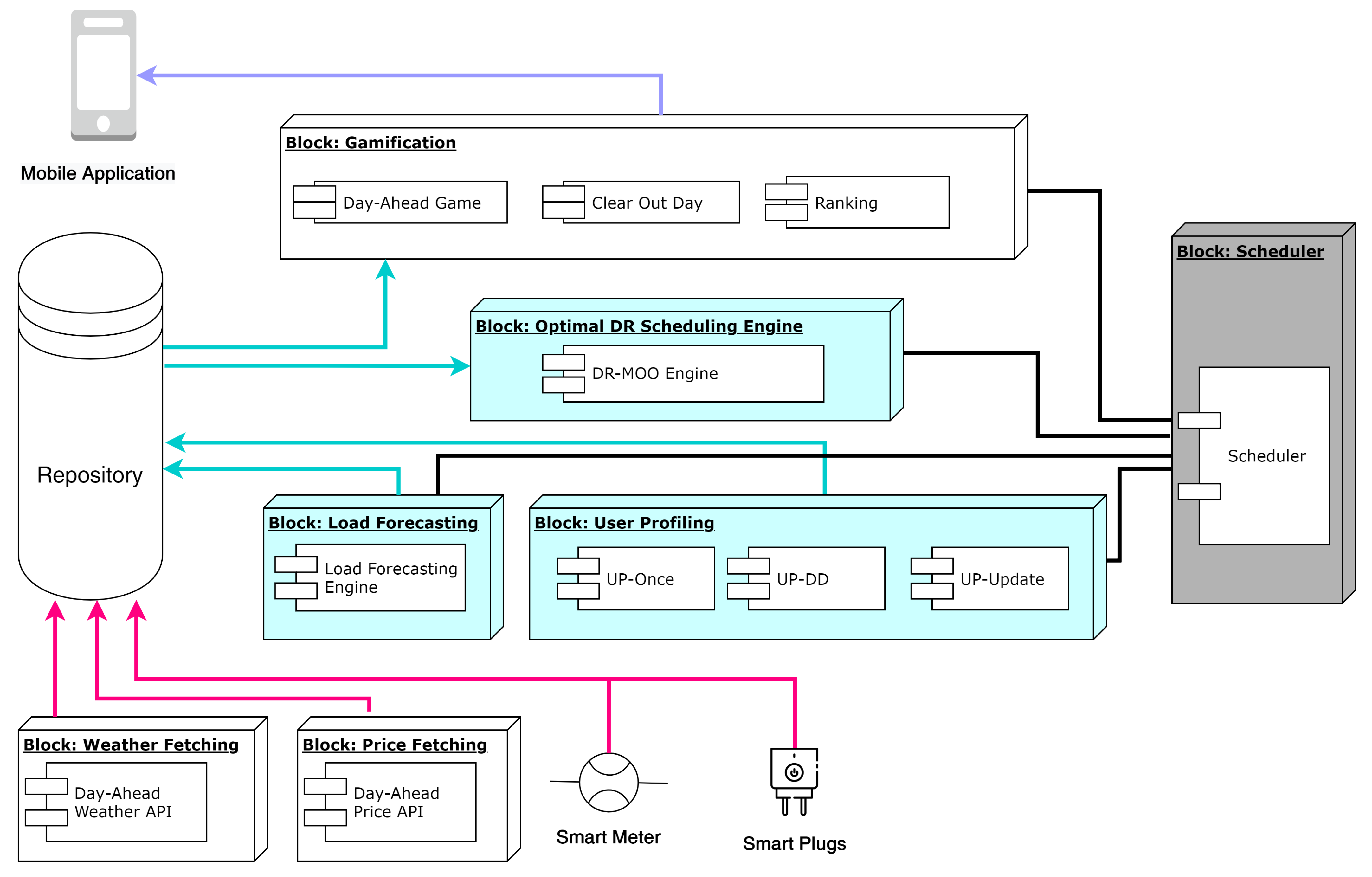
As shown in Figure 2, the proposed ODRes system is composed of several different modules, which operate sequentially and automatically. Briefly, the basic system modules are:

• The multi-objective DR optimisation engine (DR-MOO), which produces the load-shifting suggestion plan daily, which gets dispatched to the selected households from an aggregator’s portfolio;
• The Load Forecasting Engine (LFE), which is responsible for defining the day-ahead consumption forecast of each household of a portfolio;
• The User Profiling (UP), which defines the shiftable electrical devices in each household, based on the residents’ preferences and the actual measurements collected daily.

Apart from these core components, the ODRes system is complemented by (a) a simple gamification engine which is responsible for implementing a point-based competition game among the participating users; (b) a mobile application which communicates the suggested optimal appliance usage plan to the users; (c) a scheduler that coordinates the operation of the aforementioned modules so that the overall ODRes system operates in a fully automated manner without human interference; and (d) a web-based user-interface (UI) which is used by the actor, that is, the aggregator, in order to provide an overview of the system’s operation and its economic evaluation. Given the fact that these complementary modules do not contain any significant innovation and they assist in the application and evaluation of the ODRes system, they are briefly discussed. In the following paragraphs, a detailed description of the core system components is given.

2.2. Optimal DR Dispatch

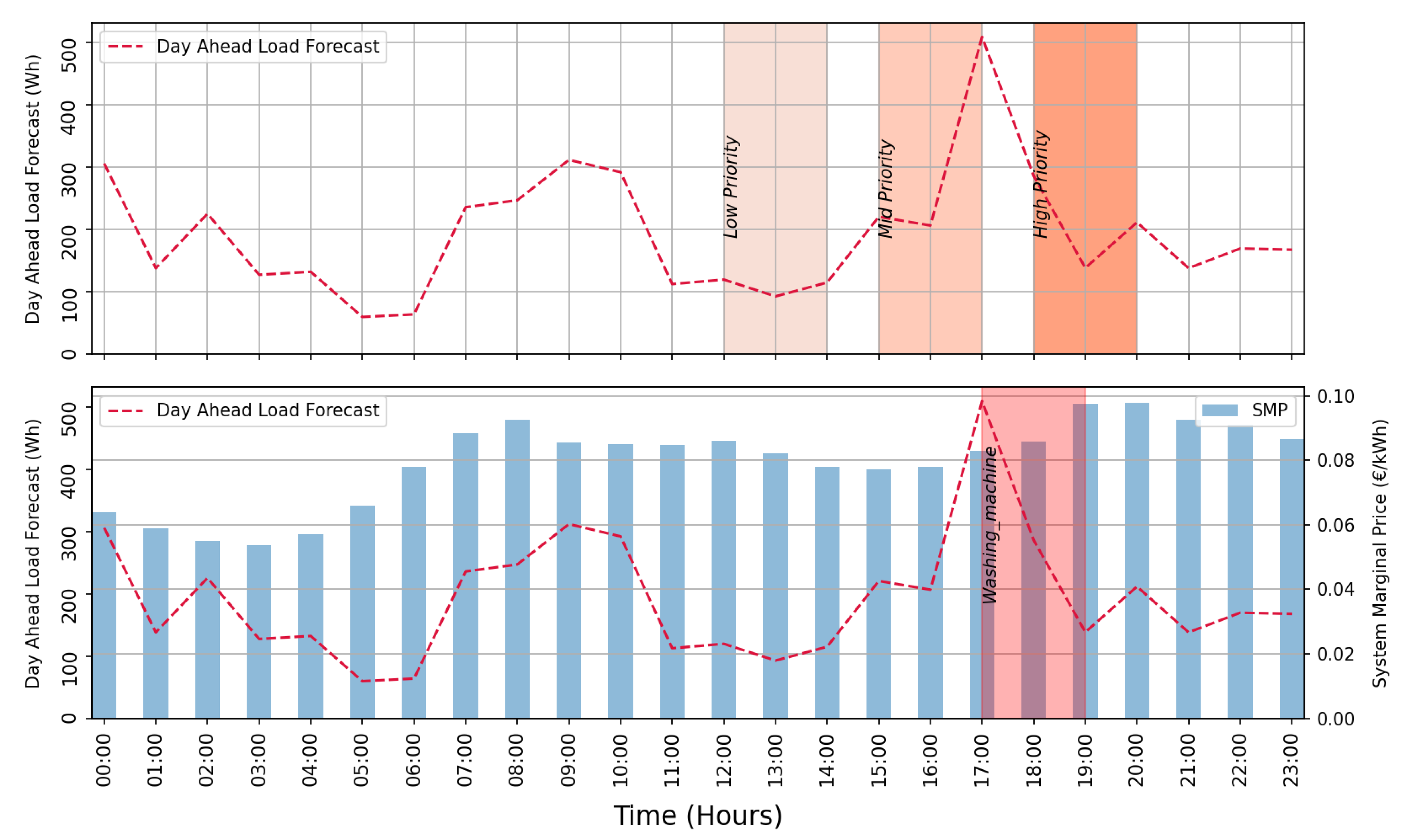
The aim of the proposed DR strategy is to reduce the overall 24-h electricity cost by providing the end-user with suggestions in order to schedule some of their shiftable appliances’ operation in specific periods within a day. Dynamic pricing is utilised, since the actor is the energy retailer, that is, the aggregator. One of the auxiliary modules that is quite significant for the optimal DR strategy is the user’s DR activity/engagement profiling which reflects every consumer’s preferences and activities affecting home habits, for example, cooking and washing, and information with respect to their infrastructures. Aiming to create a realistic optimal scheduler for this scenario, the multi-objective optimisation engine must take into consideration a series of factors:

• The specific characteristics and preferences of each particular consumer;
• The day-ahead System Marginal Price (SMP), that is, the electricity wholesale hourly price produced by relevant national bodies such as energy market operators;
• The day-ahead load forecast for each particular household;
• The appliances’ usage preferences of the household residents;
• The appliances’ consumption signatures (timeseries).

The multi-objective optimisation problem is formulated using Mixed-Integer Linear Programming (MILP). The optimised scheduler can redistribute only the most deferrable appliances in each household, that is, dishwasher, laundry machine, water boiler and so forth. Based on the day-ahead load forecast, it detects the time intervals in which a high energy-consuming appliance is on and attempts to reschedule it to a less costly time slot, producing a variety of different options. As soon as all the possible schedules have been retrieved for each individual consumer, aggregated optimisation is applied for the whole portfolio, using the DR activity/engagement profiling, based on past records of the consumers on previous DR engagement and current DR participation. The final output of DR-MOO is the group of consumers that have been selected to participate in the day-ahead DR scheduling, including the individual suggested plans for each household.

The mathematical formulation of the DR-MOO problem is given in Equation (1). The objective function is composed of two terms that are both minimised. The first term, ${\mu }_1\left(\mathbf{O}\right)$, corresponds to the total cost of the daily consumption of a household within the aggregator’s portfolio, while the second term, ${\mu }_2\left(\mathbf{O}\right)$, models the total dissatisfaction of the household residents deriving from the suggested load shifts. The objective function is subjected to three constraints: (a) by the first one, the overall household consumption is barred by a maximum limit, which essentially corresponds to the household’s contracted power if it was absorbed continuously during one hour ($L_{max}$, in kWh); (b) given the fact that load shifting is pursued, the total daily energy consumption must remain the same; and, finally, (c) each appliance can be shifted only once and to time slots that are within the users’ preferences. The symbol ⊙ corresponds to the Hadamard (or element-wise) product of the matrices.

$$\begin{array}{cc}\hfill \underset{\mathbf{O}}{min}& {\mu }_1\left(\mathbf{O}\right),{\mu }_2\left(\mathbf{O}\right)\hfill \\ \hfill \mathrm{where}& {\mu }_1\left(\mathbf{O}\right)={({\mathbf{L}}_{\mathbf{sh}}\odot \mathbf{O}·{\overrightarrow{J}}_{N·P_N}+\overrightarrow{L_b})}^{⊺}·\overrightarrow{C}\hfill \\ \hfill & {\mu }_2\left(\mathbf{O}\right)=\mathbf{O}\odot \mathbf{D}·{\overrightarrow{J}}_{N·P_N}·{\overrightarrow{J}}_T\hfill \\ \hfill \mathrm{s}.\mathrm{t}.& {\overrightarrow{L_{sh}}}^{⊺}·\mathbf{O}+{\overrightarrow{L_b}}^{⊺}\le {\overrightarrow{L_{max}}}^{⊺}\hfill \\ \hfill & \sum _{c=1}^{c_{n_{\delta }}}\frac{{\sum }_{t=1}^T{o}_{t,c}}{∥max\left(l_{*,c}\right)∥}=1\forall \delta \in [1,N],\hfill \end{array}$$

(1)

where

• $\mathbf{O}=\left[\begin{array}{ccccccccc}\hfill o_{t,c=(1,1)}^{n=1}& \cdots & o_{t,c=(1,c_{n_1})}^{n=1}\hfill & o_{t,c=(1,1)}^{n=2}& \cdots & o_{t,c=(1,c_{n_2})}^{n=2}& o_{t,c=(1,1)}^{n=N}& \cdots & o_{t,c=(1,c_{n_N})}^{n=N}\\ \hfill ⋮& \ddots & ⋮\hfill & ⋮& \ddots & ⋮& ⋮& \ddots & ⋮\\ \hfill o_{t,c=(T,1)}^{n=1}& \cdots & o_{t,c=(T,c_{n_1})}^{n=1}\hfill & o_{t,c=(T,1)}^{n=2}& \cdots & o_{t,c=(T,c_{n_2})}^{n=2}& o_{t,c=(T,1)}^{n=N}& \cdots & o_{t,c=(T,c_{n_N})}^{n=N}\end{array}\right]$
  contains the optimisation variables; it is a $T\times N·P_N$-sized matrix with binary elements, where N is the number of shiftable appliances in a household, T is the number of total time slots of the optimisation horizon (e.g., 24, 96 with hourly, quarterly resolution etc.) and $P_N$ is the number of total possible permutations of all devices; the dashed separators of the table signify the $c_n$ columns corresponding to appliance n and the total number of possibilities in which it can appear; $o_{i,j}$ is equal to 1 if the device is selected to be operating, otherwise it is 0; the indices t,c correspond to time slot and the permutation of appliance n;
• ${\mathbf{L}}_{\mathbf{sh}}=\left[\begin{array}{ccccccccc}\hfill l_{t,c=(1,1)}^{n=1}& \cdots & l_{t,c=(1,c_{n_1})}^{n=1}\hfill & l_{t,c=(1,1)}^{n=2}& \cdots & l_{t,c=(1,c_{n_2})}^{n=2}& l_{t,c=(1,1)}^{n=N}& \cdots & l_{t,c=(1,c_{n_N})}^{n=N}\\ \hfill ⋮& \ddots & ⋮\hfill & ⋮& \ddots & ⋮& ⋮& \ddots & ⋮\\ \hfill l_{t,c=(T,1)}^{n=1}& \cdots & l_{t,c=(T,c_{n_1})}^{n=1}\hfill & l_{t,c=(T,1)}^{n=2}& \cdots & l_{t,c=(T,c_{n_2})}^{n=2}& l_{t,c=(T,1)}^{n=N}& \cdots & l_{t,c=(T,c_{n_N})}^{n=N}\end{array}\right]$
  is a $T\times N·P_N$-sized matrix corresponding to each appliance’s consumption signature (in kWh), that is, the energy that is consumed every hour of operation by each shiftable appliance calculated according to the collected measurements; following the same structure as for $\mathbf{O}$, each column corresponds to the n-th appliance consumption signature starting and ending at different time slots;
• $\mathbf{D}=\left[\begin{array}{ccccccccc}\hfill d_{t,c=(1,1)}^{n=1}& \cdots & d_{t,c=(1,c_{n_1})}^{n=1}\hfill & d_{t,c=(1,1)}^{n=2}& \cdots & d_{t,c=(1,c_{n_2})}^{n=2}& d_{t,c=(1,1)}^{n=N}& \cdots & d_{t,c=(1,c_{n_N})}^{n=N}\\ \hfill ⋮& \ddots & ⋮\hfill & ⋮& \ddots & ⋮& ⋮& \ddots & ⋮\\ \hfill d_{t,c=(T,1)}^{n=1}& \cdots & d_{t,c=(T,c_{n_1})}^{n=1}\hfill & d_{t,c=(T,1)}^{n=2}& \cdots & d_{t,c=(T,c_{n_2})}^{n=2}& d_{t,c=(T,1)}^{n=N}& \cdots & d_{t,c=(T,c_{n_N})}^{n=N}\end{array}\right]$
  is the $T\times N·P_N$-sized matrix which contains the preferences of a household’s residents regarding the operation of the available shiftable N appliances and all their possible permutations $c_{n_N}$ within one day with a total of T time slots. The preferences of the users are modelled as integers;
• $\overrightarrow{L_b}=\left[\begin{array}{c}{L}_{b_1}\\ ⋮\\ L_{b_T}\end{array}\right]$ is a T-sized vector corresponding to the baseline (non-shiftable) daily consumption (in kWh) of a household;
• $\overrightarrow{C}=\left[\begin{array}{c}{C}_1\\ ⋮\\ C_T\end{array}\right]$ is a T-sized vector containing the varying energy price of the day; given the fact that the actor of the proposed ODRes is the Aggregator, then this price corresponds to the SMP, based on which the actor buys energy;
• ${\overrightarrow{J}}_T,$${\overrightarrow{J}}_{N·P_N}$ are unitary vectors, sized T and $N·P_N$, respectively.

The optimisation problem described above is solved for every household in the portfolio. For each household, a Pareto front is extracted as the result of the optimisation, which contains the set of optimal solutions which correspond to different combinations of cost and overall user satisfaction. In order to select one optimal solution for each household, a heuristic logic is followed: for each household user, an engagement index is assigned, which is an integer indicating how responsive they are to DR participation. For example, if the household user has been actively, moderately or minimally engaged, they are assigned a value of three, two or one, respectively. Additionally, another index is considered that represents the most recent participation of the household. For example, the value three is assigned if the household participated in yesterday’s DR, two for the day before and one for any previous day prior. The product value of these two indices is named the Schedule Selector Index (SSI), and is considered in the optimisation process. This process is depicted with the help of

Table 1. Schedule Selector Index Look-up Table.

		Last Participated
		3 (Today-1)	2 (Today-2)	1 (Today-3)
ine	1	3	2	1
Resident’s Engagement Index	2	6	4	2
	3	9	6	3

. It is noted that the cells coloured in the darkest grey lead to maximised profit for the aggregator, the white cells offer minimised user dissatisfaction and the cell in the middle is the compromise between the two objectives.

2.3. User Profiling

The user profiling module (UP) is the main component for extracting all the meaningful information about electrical appliances in each household. Home appliance information is based on residents’ preferences and the analysis of daily electrical measurements. The user profiling module consists of three sub-modules, namely the UP-once, the UP-dd and the UP-update sub-modules. Each one of these performs the necessary functions required to obtain the maximum information related to the operation of electrical appliances.

2.3.1. UP-Once

This sub-module is initiated in order to process and store the initial preferences for each participating household. In particular, preferences were obtained in the form of an online structured questionnaire, which registers information regarding the electrical appliances’ usage, prior to the implementation of the proposed technique. In addition, the consumer can state the intervals in order of priority regarding the use of the electrical appliance. More specifically, preferences are classified into three categories, namely low, medium and high order of priority. The questions are formulated in such a way that gives the opportunity to the aggregator to have an initial estimate of the energy consumption of each household before the installation of the smart meters. Additional demographic questions are included, to identify whether the residents are a working couple, a student, a retired couple or a multi-generational family, as the daily routines and the schedule of each type differs significantly within the day, having a direct impact on their energy consumption. The residents are also required to answer a series of questions regarding the appliances that they wish to register as shiftable, along with some general questions that help UP-once better identify each appliance’s signature (e.g., age, size etc.). The users are then asked to fill in the time intervals in which they prefer to use their electrical appliances within a working and a weekend day. After completing the questionnaire, an automated parsing and transcoding of the respective answers is conducted in order to be used as input to the optimisation engine.

2.3.2. UP-DD

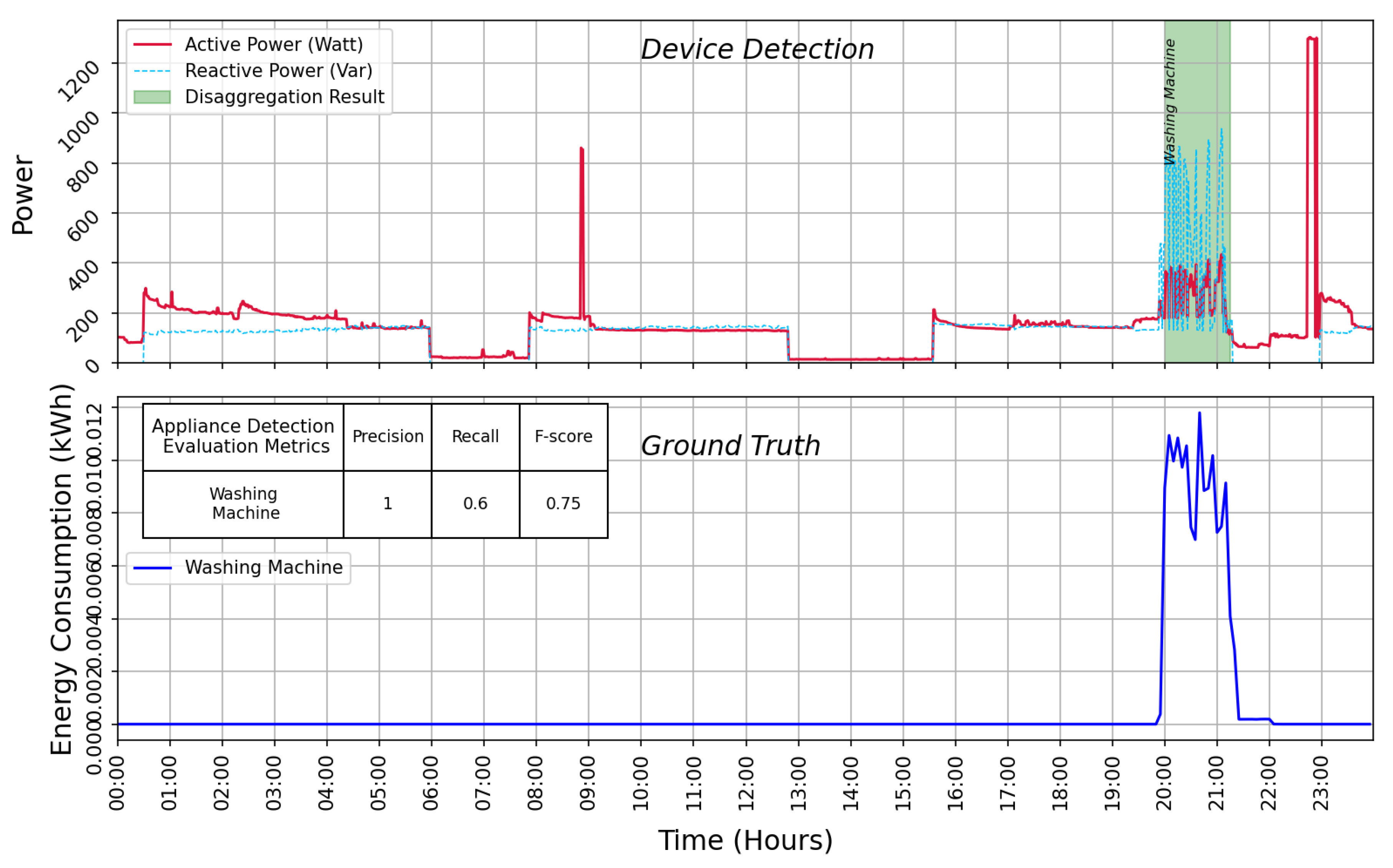
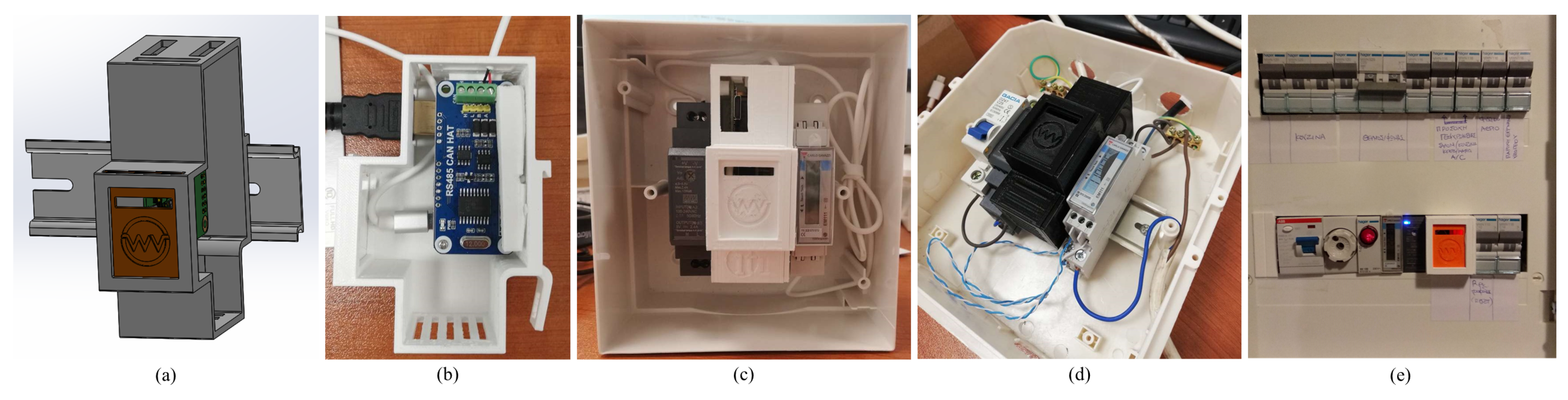
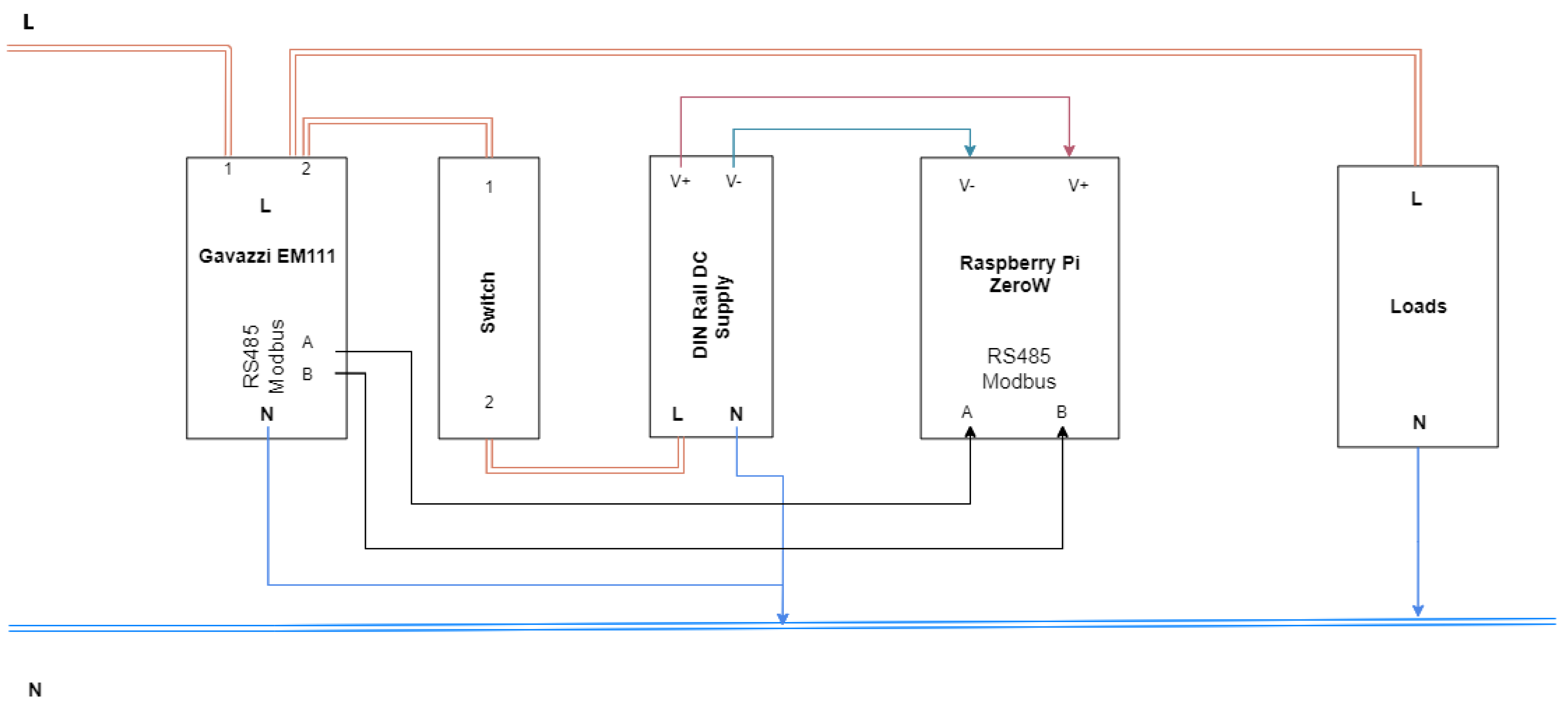
This sub-module is executed on a daily basis and is in charge of the detection of the time intervals in which each device has been operational. In particular, a non-intrusive load monitoring (NILM) algorithm was developed, which disaggregates the total household power consumption into individual appliances’ consumption [26]. In the context of the current work, a total of four appliances were selected for disaggregation: (1) Oven, (2) Washing machine, (3) Dishwasher and (4) Dryer. Smart plugs were installed to those appliances of the participating households in order to gather baseline data which are necessary for the training of the supervised disaggregation models. The data gathering period lasted approximately one month. Data consistency and completeness were thoroughly checked, as missing values may create a loss of temporal sequence in time-series data and valuable information may be lost. Consequently, only the days with more than 90% of available data were kept, while the missing values were linearly interpolated. The total consumption is given from smart meters installed on the main panel of each household. The active power (P) and reactive power (Q) are utilised as input features for the disaggregation problem. Reactive power is an informative feature for the four selected appliances, since their electrical behaviour is non-ohmic, so the reactive component of power is critical for distinguishing the appliance’s signature from the whole household’s consumption. The temporal changes of total P and Q also play a crucial role in the recognition of an appliance’s pattern. Thus, a configurable number of historical timestamps is defined for each appliance model and those instances are used as additional features. The number of historical timestamps is different for each appliance model and it depends on the appliance’s operational cycle. The temporal features are described mathematically by the following equations:

$$\begin{array}{c}\hfill P_{diff,i}=P_{t-i},i=1,\cdots ,H\end{array}$$

(2)

$$\begin{array}{c}\hfill Q_{diff,i}=Q_{t-i},i=1,\cdots ,H,\end{array}$$

(3)

where $P_{diff,i}$ and $Q_{diff,i}$ are the active and reactive power, respectively, at timestamp i and H is the number of historical timestamps that are used as features.

Apart from the electrical features, it was also attempted to extract information from the hourly and daily patterns of usage. An encoding process was followed in order to model those features which are related to the periodical use of the appliances. They were first transformed cyclically into sines and cosines representations and were then mapped onto a circle in order to preserve the proper relationships between them.

$$\begin{array}{cc}\hfill hour\_sin& =sin(2\pi ·hour/23),0\le hour\le 23\hfill \end{array}$$

(4)

$$\begin{array}{cc}\hfill hour\_cos& =cos(2\pi ·hour/23),0\le hour\le 23\hfill \end{array}$$

(5)

$$\begin{array}{cc}\hfill day\_sin& =sin(2\pi ·day/364),0\le day\le 364\hfill \end{array}$$

(6)

$$\begin{array}{cc}\hfill day\_cos& =cos(2\pi ·day/364),0\le day\le 364\hfill \end{array}$$

(7)

A supervised regression model approach was utilised for the estimation of the exact consumption value of the appliances that were being disaggregated. A tree-based technique was selected, having as a criterion high accuracy combined with low computational cost. More specifically, the Extreme Gradient Boosting (EGB) algorithm was used, which is analysed in detail in Section 2.4.

2.3.3. UP-Update

This is the final sub-module of the UP component and it is executed on a monthly basis updating the base load value, the maximum consumption and the preferences regarding the electrical appliances of each household. The base load is defined as the minimum amount of energy needed by each household, in other words, it corresponds to all the inflexible appliances of a house (e.g., fridge, TV etc.). Both base load and maximum consumption are estimated by conducting a statistical analysis of the actual measurements received by the smart meters. Hence, as the goal of the DR strategy is load shifting, the base load and the maximum consumption are two important factors in determining which time slots are suitable for shifting device operation. In addition, as mentioned above, energy consumption is generated by the use of devices through a set of “practices”, which can be interpreted as a series of actions governed by different motives and intentions of residents [27]. These practices correspond to the daily routine activities and are likely to change over time. Thus, the initial residents’ preferences that are based on the routine activities may be incorrect. Therefore, a statistical analysis was conducted on the results of the UP-dd module and new preferences were extracted and stored to the database.

2.4. Load Forecast

Day-ahead load forecast is considered a multi-step time series forecasting problem, and as the name implies, the prediction of multiple steps ahead is required. In general, two methods are the main approaches for multiple time series forecasting [28], namely the recursive and the direct multi-step forecast strategy. The recursive multi-step forecast utilises the forecasted value of the prior time step as the input for the next forecast. The main disadvantage of this approach is that the use of forecasted values as new observations leads to performance degradation due to the accumulation of the forecast’s errors as the forecast horizon increases. The direct strategy, which is adopted by the day-ahead load forecast tool of ODRes, creates a separate model for each horizon step, respectively. Having one model for each horizon step adds computational cost, but the accuracy trade-off makes this method a fitting approach.

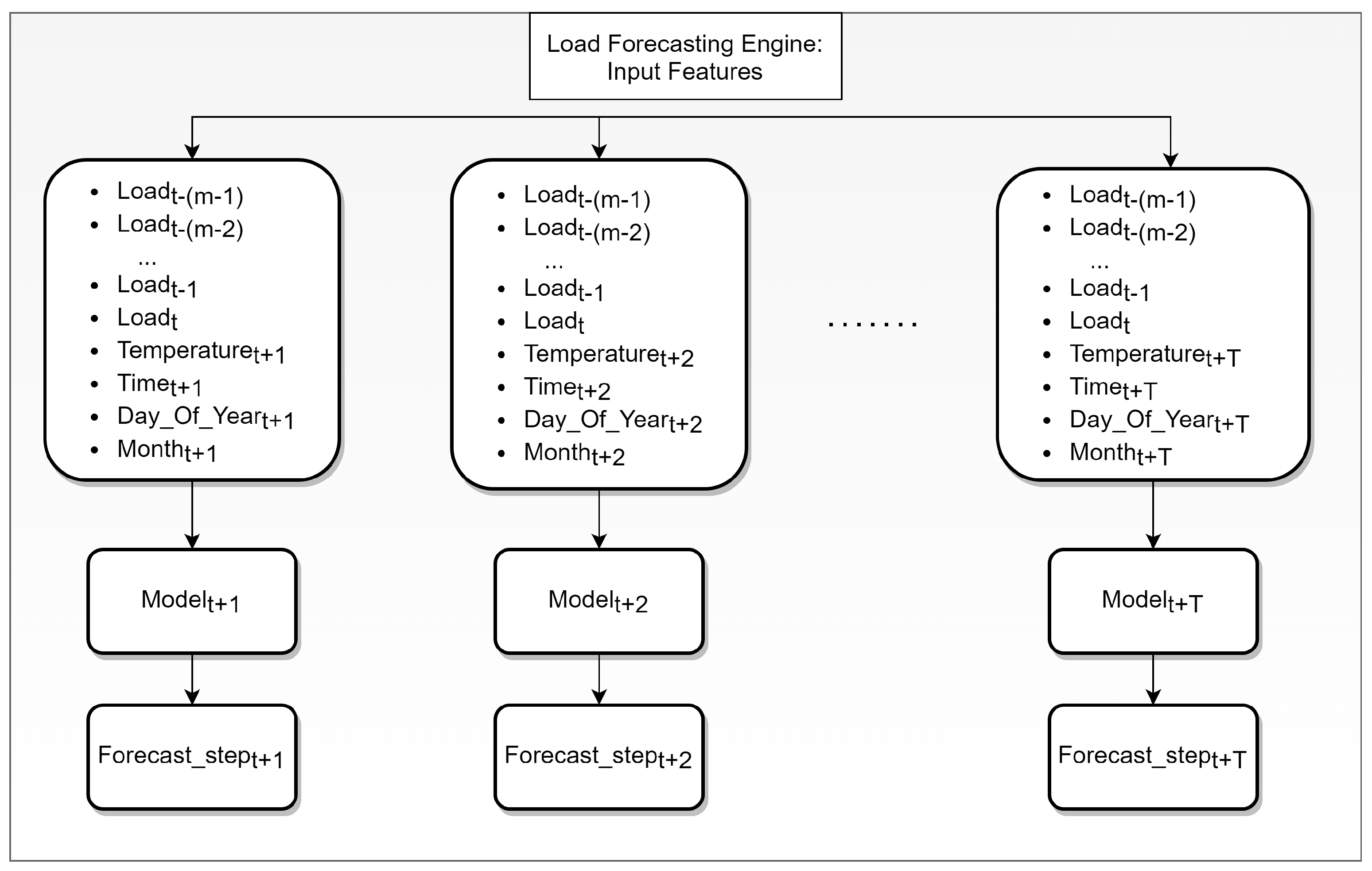
In terms of input features, as with any forecasting model, the historical values of the forecasted variable have the greatest impact on the model performance. Additionally, other external features that significantly influence the outcome, that is, the time and weather features, are integrated into the model. The time features, the so-called cyclical features, are important in order to capture the seasonality included within load consumption time series (time, day of week, month, etc.) and are encoded according to Equations (4)–() before being used as input features. As for the weather features, after a correlation analysis that was conducted, it was concluded that the outdoor temperature is the most influential among all the other weather variables and this was included in the model as well. Contrary to other methods that utilise historical values for the time and temperature features, the current work made use of the forecasted temperature and the time features that coincide with each model’s horizon step. The structure of the proposed framework regarding the input features is illustrated in Figure 3. As the training of the models was based on the direct strategy, a separate model for each time slot t was developed, while the number of the models was equal to the total time slots of the optimisation horizon T. Furthermore, the training of all the models was carried out using the same number m of past load measurements and more specifically the load measurements of the previous day (24 past measurements). Finally, the day-ahead load forecast was constructed by the total set of the individual forecasts.

The training and the development of the multiple forecast models was conducted by utilising the XGBoost library [29], which is based on the gradient boosting framework, as it has the best performance in terms of accuracy and execution time. The gradient-boosting-based model produces predictions as ensembles of multiple predictions generated by weak learners, which in this case were the decision trees. The training of the weak learners is conducted in an additive manner, each one correcting the errors made by its predecessor. The goal is the minimisation of an objective function that combines a convex loss function and a penalty term for model complexity. The final forecast is the combination of the forecast of new trees that are adjusted to the residuals of errors of prior trees and is added to the forecast of the previous tree. The simplified form of the objective function for the new tree $f_z$ of the i-th instance at the z-th iteration is:

$$\sum _{i=1}^n[g_i{f}_z\left(x_i\right)+\frac{1}{2}{h}_i{f}_z^2\left(x_i\right)]+\Omega \left(f_z\right),$$

(8)

where $g_i$ and $h_i$ are the first and second order gradient statistics of the loss function, which are defined as follows:

$$g_i={\partial }_{{\widehat{y_i}}^{(z-1)}}l(y_i,{\widehat{y_i}}^{(z-1)}),$$

(9)

$$h_i={\partial }_{{\widehat{y_i}}^{(z-1)}}^{2}l(y_i,{\widehat{y_i}}^{(z-1)}).$$

(10)

The second term of the objective function $\Omega \left(f_z\right)$ represents a regularisation term in charge of seeking the appropriate final weights to avoid over-fitting.

2.5. Auxiliary Modules

To support the functionalities of the aforementioned core components of ODRes framework, a proper backend system with some auxiliary modules is needed (see Figure 2). The scheduler is the main management tool and is responsible for executing all other tools in the right sequence in predefined time slots. The scheduler ensures the proper operation of all ODRes modules and it is enriched with a detailed logging system along with a real-time notification system which informs the system administrator in case errors occur. The scheduler is implemented in Python 3.7. In addition, there are also two modules responsible for collecting forecasts from on-line RESTful APIs provided by 3rd party service providers. These are the Weather Forecast and the Day-Ahead Electricity Price modules. The first one retrieves the predicted temperature and humidity values for the upcoming 24 h, with an hourly resolution, from the openweatherAPI platform, https://darksky.net/dev (accessed 15 June 2021), while the later retrieves the hourly wholesale electricity prices for the next day from the market operator’s online platform. The whole back-end system is supported by two complementary databases for storing timeseries and static data, that is, an influxDB and a MySQL, respectively.

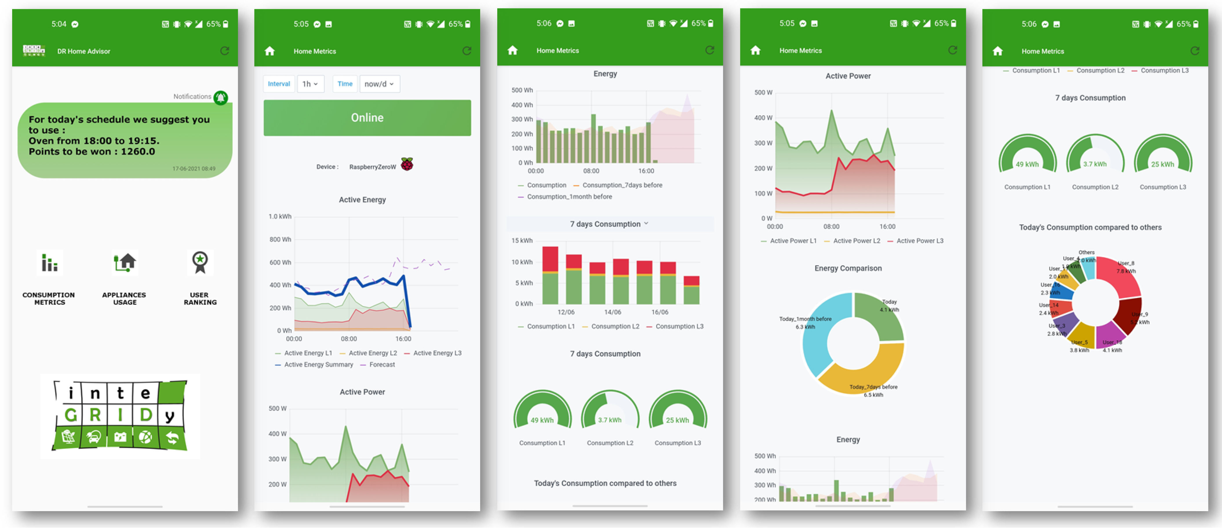
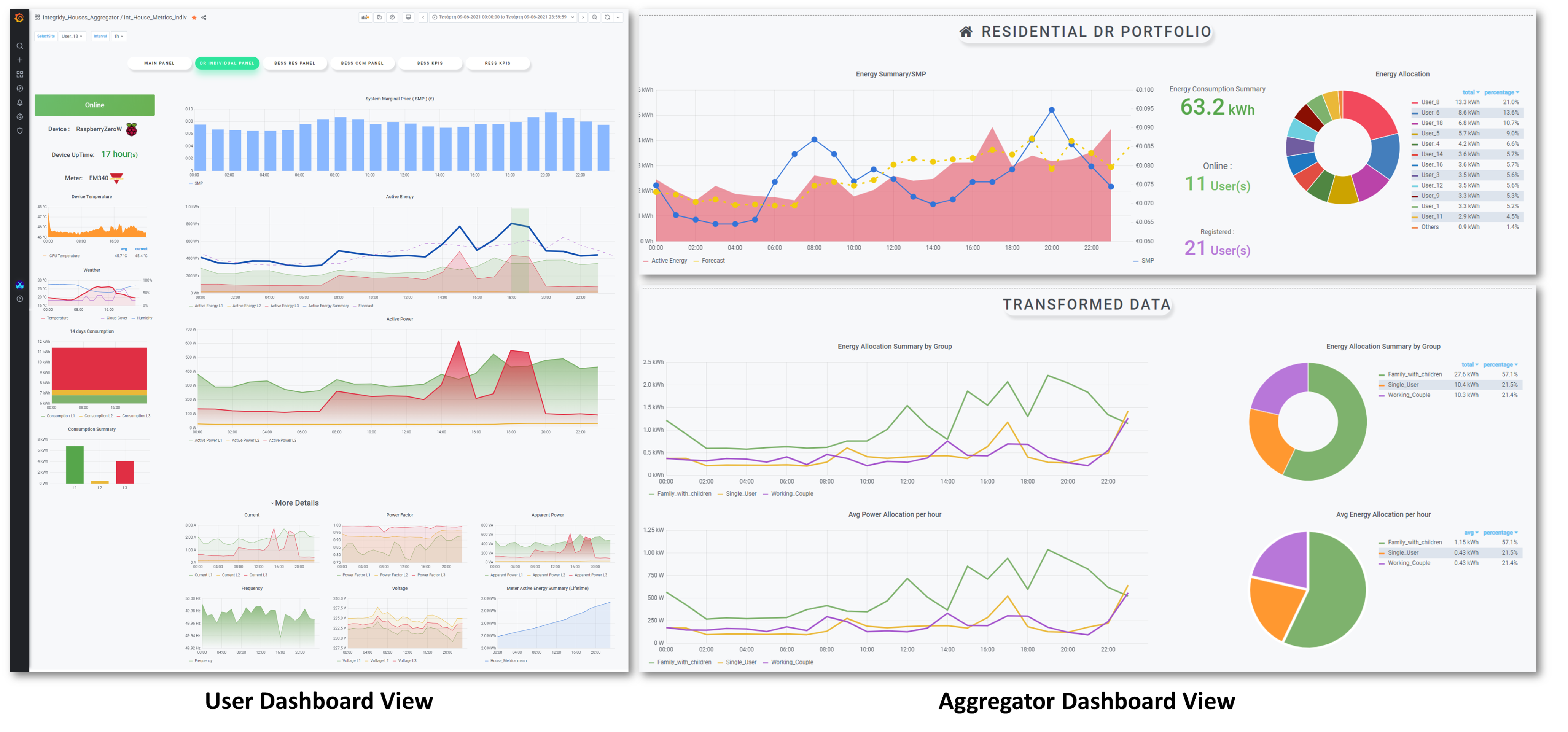
In order to create a suitable interaction environment for the ODRes framework, two front-end interfaces were developed: first, a web-based dashboard, accessible by all registered users, was designed in order to provide a full overview of the expected and implemented DR application through user-friendly and informative visual analytics. Statistical analysis of historical data, past DR application and real-time measurements were also included in the dashboard. Furthermore, a separate view of the dashboard for the aggregator was constructed in order to provide access to the whole portfolio, obtaining information in a more aggregated manner with fewer details about each user. On the other hand, a mobile Android-based application was developed so that the DR schedules were sent to the users. Google’s Firebase platform was used for signing in users and keeping them informed with Firebase Cloud Messaging (FCM), https://firebase.google.com/ (accessed 15 June 2021). Targeted messages were produced per user and sent to each registered device in the form of Android notifications, presenting an optimal schedule for the selected user’s home appliances. This procedure was executed by using Firebase’s real time database as the back-end for storing registered users and an API for the connection with the ODRes framework. The produced optimal schedule per user was stored in the ODRes MySQL database and was visualised on a graphical dashboard within the mobile application. Finally, the users could view real-time and historical measurements along with statistics regarding appliance usage deriving from the smart meters. In Figure 4 and Figure 5, screenshots of the mobile application and the web-based dashboard are shown.

3. Validation

3.1. Simulation Results

In order to validate the theoretical background of the proposed incentive-based DR scheme, simulations were performed. The size of the simulated portfolio is selected appropriately so that it is aligned also with the pilot size indicated by the H2020 inteGRIDy research project, details of which are listed in

Table 2. Simulated Houses Portfolio.

Profile	Attributes				Houses
	Residents	Appliances (Incl. Light Bulbs)	Average Daily Consumption	Shiftable Appliances
Student/Single resident	1	49	4.52 kWh	5	4
Working couple	2	65	8.55 kWh	7	26
Family-1 child	3	66	9.18 kWh	5	22
Family-3 children	5	66	14.67 kWh	6	12
Multi-generational	6	79	21.01 kWh	7	9

. The consumption time-series for each household was formulated using the open-source algorithm LoadProfileGenerator, available online: https://www.loadprofilegenerator.de (accessed 15 June 2021) [30]. Essentially, each load curve was constructed via the summation of real measurements from various appliances, scheduled appropriately as defined by each house profile. Regarding the pricing, the SMP was utilised, which was acquired from the Hellenic Energy Exchange. https://www.enexgroup.gr (accessed 15 June 2021). The simulations were carried out for a nine-month period between 1 September 2020 and 31 May 2021.

The objectives of the simulations are:

• To demonstrate the maximum theoretically achievable profit from such a DR scheme;
• To explore correlations between price fluctuations and their exploitable potential in residential incentive-based load shifting;
• To assess whether user discomfort is augmented in the case where daily profits increase.

In Figure 6, the scatter plot aims to define the correlation between daily price fluctuations, relative daily profits and average daily dissatisfaction. Each dot corresponds to each household participating in the DR scheme in one day of the simulation horizon. The continuous lines depicted in the figure are essentially the least-square trend lines. As can be observed, days characterised by high fluctuations in the SMP offer significantly larger profit margins, without however compromising user comfort, which remains relatively stable regardless of price fluctuations. This outcome is backed up not only visually from the scatter plots, but also by the calculated Pearson Correlation Coefficients, which reflect whether two variables are linearly correlated (−1 and +1 correspond to inversely proportional and proportional variables, respectively, whereas 0 implies that the variance of one variable is completely irrelevant to the variance of the other). The Pearson Coefficient between price fluctuations and relative profits is equal to +0.42, therefore a definite positive correlation between these variables is evident. On the other hand, the Pearson Coefficient between relative profits and user dissatisfaction is equal to +0.19, a fact that highlights that these two variables have practically no correlation. This finding can be considered initially as counter-intuitive, because one would assume that higher price fluctuations, which directly lead to larger profit margins from a portfolio, imply greater user dissatisfaction. However, as can be seen, this is not the case: the interpretation of this somewhat interesting phenomenon is that wholesale prices and the preferred usage timing of residential shiftable appliances are independent variables. This latter outcome is considered an asset of the proposed DR optimisation engine and, more importantly, how the comfort level of the residents (i.e., respecting their preferences) is integrated within it.

Over the simulated nine-month period, the mean daily relative profit is equal to 1.48%, with a 3.45% variance. The 0.5-Quantile (0.5Q), that is, the median of the observations, is equal to 1.14%, which is lower than the mean value, a fact that indicates that the trend is to usually achieve daily profits of less that 1.48%. The 0.75-Quantile (0.75Q) is equal to 2.19%, meaning that 25% of the observations are characterised as a considerable profit margin. The 0.25-Quantile (0.25Q) is equal to 0.3%, which in fact can be attributed as an alarming factor, since the same amount of observations (25%) can have a negligible profit. As seen in Figure 6, the days characterised by high price fluctuations are scarce, and this fact is responsible for these conservative statistical results. It is noted that a large price fluctuation does not imply in any case low or high prices; it only means that the difference between maximum and minimum price should be high enough so that the load shifting of low-power home appliances can have a positive effect on an aggregator. Though theoretically published works [6,7] advocate in favour of the unlocked potential of residential load flexibility, it becomes evident that without a proper pricing scheme, DR programmes focused on residential users will have limited business potential.

In order to explore further the effect of price to profit margins, in Figure 7, the boxplots of three variables (SMP, daily profit, portfolio usage) are given, throughout the nine simulation months. As can be observed, in December 2020, the largest price fluctuations occurred and as a result, the largest profits were achieved, without however utilising the available portfolio at its fullest. For comparison, in the months of October 2020 and similarly in April and May 2021, the reader can observe that, due to the low price fluctuations, very limited profits can be extracted even though almost the entire household portfolio is exploited.

3.2. Experimental Setup

Within the context of the H2020 inteGRIDy project, the deployment of the ODRes framework took place in selected residencies in Thessaloniki, the second largest city in Greece. To do so, customised smart meter installations had to be connected to each home’s main electrical panel. These smart meter installations were composed of: (a) a smart meter to collect the appropriate measurements (active/reactive power, energy consumption); (b) a Raspberry Zero to dispatch the aforementioned measurements to the central ODres server; and (c) a Din Rail DC power supply with an integrated safety automatic relay to power up and protect the Raspberry Zero. The single-phase houses were equipped with an Carlo Gavazzi EM111 smart meter, while the three-phase houses were equipped with a Carlo Gavazzi EM340 smart meter. The Raspberry Pi Zero W was directly connected to the smart meter and it collected all necessary measurements every minute through a Modbus RTU via the RS485 CAN HAT board. The enclosure of the device was a custom-made Din Rail case, that was created with Fused Deposition Modelling (FDM) 3D printing technology on the CERTH premises. In Figure 8 and Figure 9, the design and electrical layout of the developed solution are shown.

In addition to the previous setup, some residences were equipped with supplementary smart plugs that were attached to specific appliances in order to provide the ground truth for the UP-dd sub-module. The energy consumption measurements of these smart plugs were retrieved via a dedicated gateway and were then sent to the ODRes server via RESTful services.

Finally, with regards to the ODRes server, all modules described in Section 2, along with the web-based User Interfaces, were set up in a Linux-based machine, powered by an Uninterruptible Power Supply, the specifications of which are as follows: CPU intel cpu i7-10700k, RAM 16 GB DDR4, hard drive SSD 256GB.

3.3. Experimental Results

The experimental validation follows the same business scenario as the one presented in the simulation results in the previous section.

Table 3. Optimal DR application result. Experiment day: 9 June 2021.

Customer	Shiftable Appliance	Proposed Time Slot	Detected Time Slot	Achievement
User 1	Washing Machine	17:00–19:15	18:15–19:15	55 %
User 3	Oven	17:00–18:15	17:00–18:30	83%
User 4	Dryer	17:00–18:15	17:15–18:30	71%
User 11	Washing Machine	19:00–21:00	-	0%
User 12	Washing Machine	19:00–21:00	-	0%
User 18	Dishwasher	18:00–19:15	18:00–19:15	100%

presents the detailed results of the DR-MOO framework for six out of the ten users/houses included in the aggregator’s portfolio, which were selected for participating in the day-ahead DR schedule for 9 June 2021. The DR events were defined at midnight of the previous day, considering the day-ahead load forecast and the user’s preferences, and were extracted from the UP-Once sub-module and consequently sent as notifications through the mobile app to the end-users, containing the suggested operating time intervals of the appliances of each user, respectively. Just before the end of the day, the UP-DD sub-module detected whether the users followed the suggested appliance scheduling and estimates their participation rate (achievement), which essentially corresponds to the fraction of time actually participating in the DR process to the time dictated by the DR-MOO schedule as produced at the beginning of the day. In particular, the detection of the operating time slots of the appliance was performed at 15 minute intervals. To calculate the achievement metric, only the time slots that were within the proposed schedule were taken into consideration. If appliance operation was detected at any other time or not at all, then these slots were considered “failures”. As can be observed from column “Achievement” of Table 3, the majority of users followed the suggested plan relatively closely. It is worth mentioning that there were cases where some users ignored the suggestions despite their participation in the DR program. More specifically, there were two customers that did not follow the DR schedule at all, so their participation rate was 0%.

In order to prove the efficient operation of the proposed ODRes integrated system, the optimisation process and the results for an individual case are demonstrated in detail in Figure 10 and Figure 11. In particular, Figure 10 presents the suggested schedule of the washing machine for 1 June 2021 for one consumer, resulting from the DR-MOO engine along with the preferences related to this appliance. In Figure 11, the highlighted area depicts the output of the UP-DD sub-module, that is, the disaggregation result. This is accompanied by a second plot which shows the actual operational time interval of the respective appliance, verifying the accurate appliance detection. Additionally, Figure 10 includes all the factors that are taken into consideration during the decision making of the DR-MOO engine, namely the preferences of a particular consumer, the day-ahead SMP and the day-ahead load forecast for the respective house. It is evident that the suggested plan for the washing machine coincides with the preferences, while being in accordance with the load forecast. By observing the fluctuations of the SMP for that day, one can identify that this appliance was placed in a time slot with a relatively low price value. Both diagrams of Figure 11 showcase the high performance of the UP-DD sub module. The appliance’s operational interval is extracted utilising the results deriving from the output of NILM algorithm. It is evident that the largest part of the washing machine’s operational cycle is correctly identified. There is only one small part at the end of the operational cycle which is not identified, however this can be considered normal because this specific appliance operates at a very low active power level during that time. In general, the performance of the NILM algorithm is sufficient, considering the F-score metric (F-score = 0.75), the harmonic mean of Precision (Precision = 1) and Recall metrics (Recall = 0.6).

In order to assess the required time for the training of the load forecasting tool, one should observe its algorithmic complexity. The proposed algorithm leads to the creation of an individual set of predictive models for each household that are exclusively trained on their data. After tuning, it was decided that three months of data was needed for the initial training and construction of the static models. Those models are loaded daily, during the operation of the load forecasting tool, while they are periodically updated by performing a re-training process. Re-training is performed on a monthly basis, capturing the user’s behavioural changes in their energy usage that may depend on seasonal factors or other non-deterministic causes that can not be easily modelled. This way, the model remains up-to-date, adapting to the users’ behaviour and making sure that high quality forecasts can be generated. Similarly, the disaggregation tool utilises pre-trained models for each appliance that are also updated monthly. Consequently, the only computationally demanding process regarding the AI-based tools of the Up-Update sub-module is the initial training of the models, which requires time measured in the order of magnitude of a few minutes. The re-training process is similar to the initial training but it only occurs once a month. In daily semi-real time operation, the forecasting and disaggregation tools for each user are executed in sub-second times since no training is performed and the predictions are generated from the pre-trained models. Therefore, the framework could easily be scaled to a large number of portfolio customers for daily operation.

4. Conclusions & Future Work

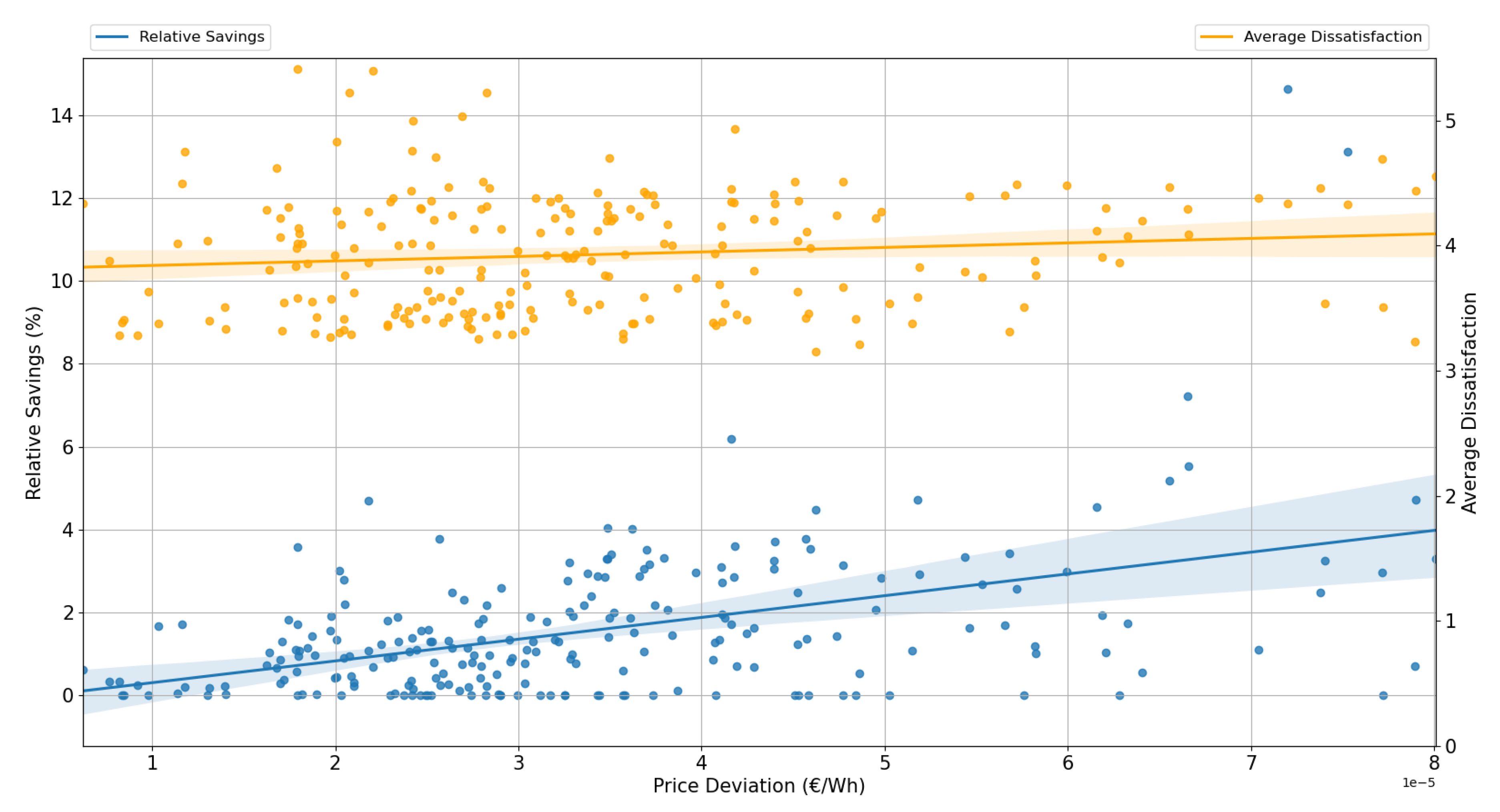
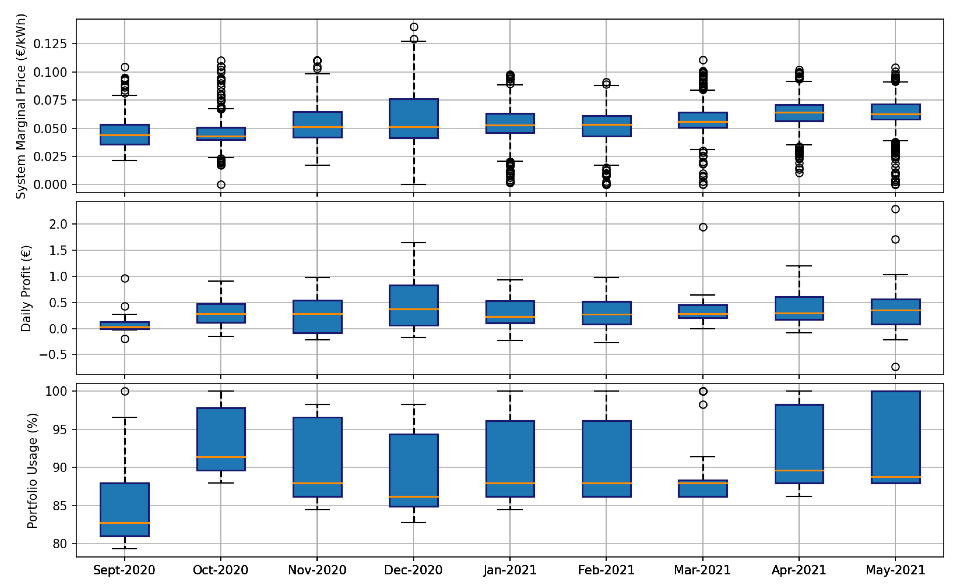
Exploiting the hidden flexibility potential within the residential sector is still a daunting task as opposed to industrial or commercial users. Configuring the most apt optimised DR schedule has very limited real-life demonstration, despite the large amount of published research. To that end, this work presented a holistic incentive-based DR framework (ODRes) for load shifting. The ODRes framework is composed of several components which employ several different technologies, including optimisation techniques, machine learning, data analytics, hardware and mobile and web-based user interfaces. Three key innovations are incorporated in the core components of the ODRes system: (a) the multi-objective DR scheduling problem, which performs cost minimisation while considering end-user comfort preferences; (b) appliance disaggregation, which aims towards identifying specific household appliances via the analysis of quarterly aggregated energy consumption based on pre-defined appliance signature models; and, finally, (c) the residential load forecasting, which is based not only on historical measurements but also upon the day-ahead weather predictions, leading to more accurate results. One major innovative aspect of the presented work is the fact that its performance has been evaluated both in simulations and in real houses in Thessaloniki, Northern Greece. From the performed simulations, the mean daily profit is 1.48% with a 3.45% variance. This is the theoretical maximum profit that can be extracted by a small portfolio with only four shiftable appliances considered. As proven by the simulation analysis, these profits are directly correlated to the price fluctuations, implying that, in the future, pricing schemes with larger deviations will lead to significantly larger profit margins deriving from residential incentive-based DR. To test the applicability of the proposed framework to real households, ten houses in Thessaloniki were used as a testbed. The ODRes system was deployed in a server to run all modules automatically, smart meters were installed on each house’s main electrical panel along with some smart plugs, while a small mobile application was developed in order for the system to interact with the users. The experimental results are promising with regards to both the performance of the overall ODRes system and the business potential.

The simulation and experimental results highlight the roadmap to future work. More specifically, to address the potentially limited user participation, the development of an innovative and more appealing gamification engine could lead to increased user engagement with the DR program, achieving behavioural change targeted towards residential energy efficiency. Furthermore, to increase profit margins, the authors have considered expanding the number of devices included for DR, such as water heaters and residential HVAC systems (heat pump, AC etc.). The DR portfolio is also considered to be expanded to include more households and to investigate potential issues at larger scales. These would also lead to an expansion of the combination of devices to be identified by the disaggregation tool. A trial of other techniques (e.g., hidden factorial Markov Models, Support Vector Machines, unsupervised learning) regarding load forecasting and disaggregation could be considered for utilisation for households with and without the smart plugs connected to the related devices. Additionally, a comparative analysis of the proposed approach while using other DR schemes, such as DLC—or even with different DR strategies, for example, ToU or CPP—is to be examined as well. A final interesting aspect that could be explored is the multi-objective optimisation engine, which could be implemented using stochastic optimisation and metaheuristic methods to improve its performance for large aggregator portfolios.