Article

A Combined Fuzzy GMDH Neural Network and Grey Wolf Optimization Application for Wind Turbine Power Production Forecasting Considering SCADA Data

by
Azim Heydari
1,*,
Meysam Majidi Nezhad
1,
Mehdi Neshat
2,
Davide Astiaso Garcia
3,
Farshid Keynia
4,
Livio De Santoli
1 and
Lina Bertling Tjernberg
5
1
Department of Astronautical, Electrical and Energy Engineering (DIAEE), Sapienza University, 00184 Rome, Italy
2
Optimization and Logistics Group, School of Computer Science, University of Adelaide, Adelaide 5005, Australia
3
Department of Planning, Design, and Technology of Architecture, Sapienza University of Rome, 00197 Rome, Italy
4
Department of Energy Management and Optimization, Institute of Science and High Technology and Environmental Sciences, Graduate University of Advanced Technology, Kerman 7631133131, Iran
5
School of Electrical Engineering and Computer Science, KTH Royal Institute of Technology Stockholm, 10044 Stockholm, Sweden
*
Author to whom correspondence should be addressed.
Energies 2021, 14(12), 3459; https://doi.org/10.3390/en14123459
Submission received: 7 May 2021 / Revised: 2 June 2021 / Accepted: 9 June 2021 / Published: 11 June 2021
(This article belongs to the Special Issue GIS and Remote Sensing for Renewable Energy Assessment and Maps)

Abstract

:
A cost-effective and efficient wind energy production trend leads to larger wind turbine generators and drive for more advanced forecast models to increase their accuracy. This paper proposes a combined forecasting model that consists of empirical mode decomposition, fuzzy group method of data handling neural network, and grey wolf optimization algorithm. A combined K-means and identifying density-based local outliers is applied to detect and clean the outliers of the raw supervisory control and data acquisition data in the proposed forecasting model. Moreover, the empirical mode decomposition is employed to decompose signals and pre-processing data. The fuzzy GMDH neural network is a forecaster engine to estimate the future amount of wind turbines energy production, where the grey wolf optimization is used to optimize the fuzzy GMDH neural network parameters in order to achieve a lower forecasting error. Moreover, the model has been applied using actual data from a pilot onshore wind farm in Sweden. The obtained results indicate that the proposed model has a higher accuracy than others in the literature and provides single and combined forecasting models in different time-steps ahead and seasons.

1. Introduction

Wind power industries have been tremendously expanded and are expected to progress at a compound annual growth rate (CAGR) of 5.2% between 2020 and 2027. This extension resulted in the produced power cost of wind energy as one of the most significant renewable and low-carbon energy resources. Wind power generation is currently one of the principal renewable energy power generations [1,2,3,4]. Wind energy is stochastic, uncertain, and discontinuous, antagonistically influencing the power grid’s protected and stable activity and the nature of the power supply [5]. The stochasticity and discontinuity of wind power could diminish the reliability prediction system and wind power quality [6].
A potential answer to these issues is to improve the forecast accuracy of wind generation. Several studies [7,8,9,10,11,12] are proposed to portray the distribution of the wind power prediction, and diverse scientific methodologies are connected to improve its accuracy. Other studies proposed complex models such as the Laplace distribution [9], the Beta distribution [10], the hyperbolic distribution [11], the Levy α-stable distribution [12], and the flexible likelihood distribution [13], which have been proposed to improve the fitting precision of the wind power prediction. In the previous decade, many studies to assess and predict the various aspects of energy management and power systems have been presented. For example, wind and solar power generation forecasting [14,15,16], condition monitoring of wind turbines [17], electricity market [18], and load forecasting [19,20] are proposed. Amjady et al. (2011) provided the short-term wind power prediction dependent on the ridgelet neural network (RNN) with a high capacity estimate ability. They suggested a differential evolution algorithm with a new selection mechanism and crossover to train the network [21]. Han et al. (2017) proposed combined models based on autoregressive integrated moving average (ARMA) and non-parametric model for wind speed forecasting [22].
The results demonstrated that non-parametric based combined models usually have a better performance than other models. Jonas C. Pelajo et al. (2019) developed a model to predict wind speed and energy price to determine the optimal maintenance planning of a real wind farm in the Brazilian Northeast [23]. Osório et al. (2014) proposed a combined forecasting model based on mutual information, wavelet transform, particle swarm optimization, and adaptive neuro-fuzzy inference system framework to predict the short-term wind power and electricity market prices [24]. Gallego-Castillo et al. (2016) provided a quantile relapse model dependent on the recreating piece Hilbert space (RKHS) system to predict the wind power probabilistic. Furthermore, they implemented two types of models (online and offline) for a real wind farm [25]. Xiao et al. (2017) employed an electrical power system prediction model using a wavelet neural network (WNN) model and an improved cuckoo search algorithm. The results showed that the proposed model essentially diminished the expectation error with respect to other relative models [26].
Kunpeng Shi et al. (2018) provided a combined model based on two-stage feature selection and improved random forest models to short term wind power forecasting [27]. Van Quang Doan et al. (2019) have presented a mesoscale ensemble model to predict wind speed ramps. The proposed model applied at real wind farms in Japan [28]. Duan et al. (2021) developed a combined intelligent model based on the improved variational mode decomposition and Correntropy long short-term memory neural network to predict wind power. The model was evaluated using two wind farms in China at different sampling intervals [29]. Yildiz et al. (2021) presented a two-step new deep learning approach based on the variational mode decomposition (VMD) method and modified the residual-based deep convolutional neural network for wind power forecasting [30]. Jafarzadeh et al. (2021) provided a modified fuzzy wavelet neural network for short-term wind power forecasting considering weather and power plant parameters. In order to evaluate the model, the Mnjil wind power plant in Iran has been used [31].
In addition, GIS-based models play an important role in renewable energy potential assessment and prediction [32,33]. Furthermore, the behavior and performance of renewable energy systems can be estimated using GIS models [34,35].
Generally, in order to model the wind turbine power production analysis, a combined intelligent solution is required. It means that the data should first be modelled by a combined data pre-processing model then a combined intelligent strategy should analyze the processed data. This type of strategy plays an essential role in managing the energy production of wind farms.
In this research, we propose an integrated strategy that couples an empirical mode decomposition, fuzzy GMDH (group method of data handling) neural network, and grey wolf optimization algorithm (GWO) to forecast the produced power of wind turbines. Furthermore, to detect and clean outliers, a combined K-means and density-based local outliers (LOF) are applied.
The main contributions and novelty of this paper are illustrated as follows:
(a)
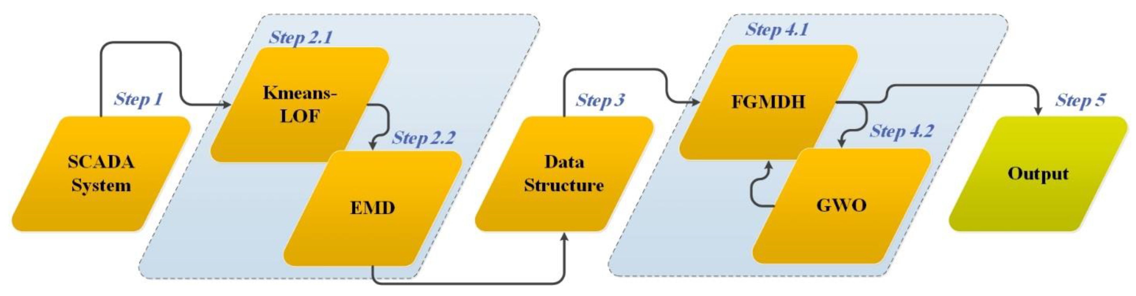
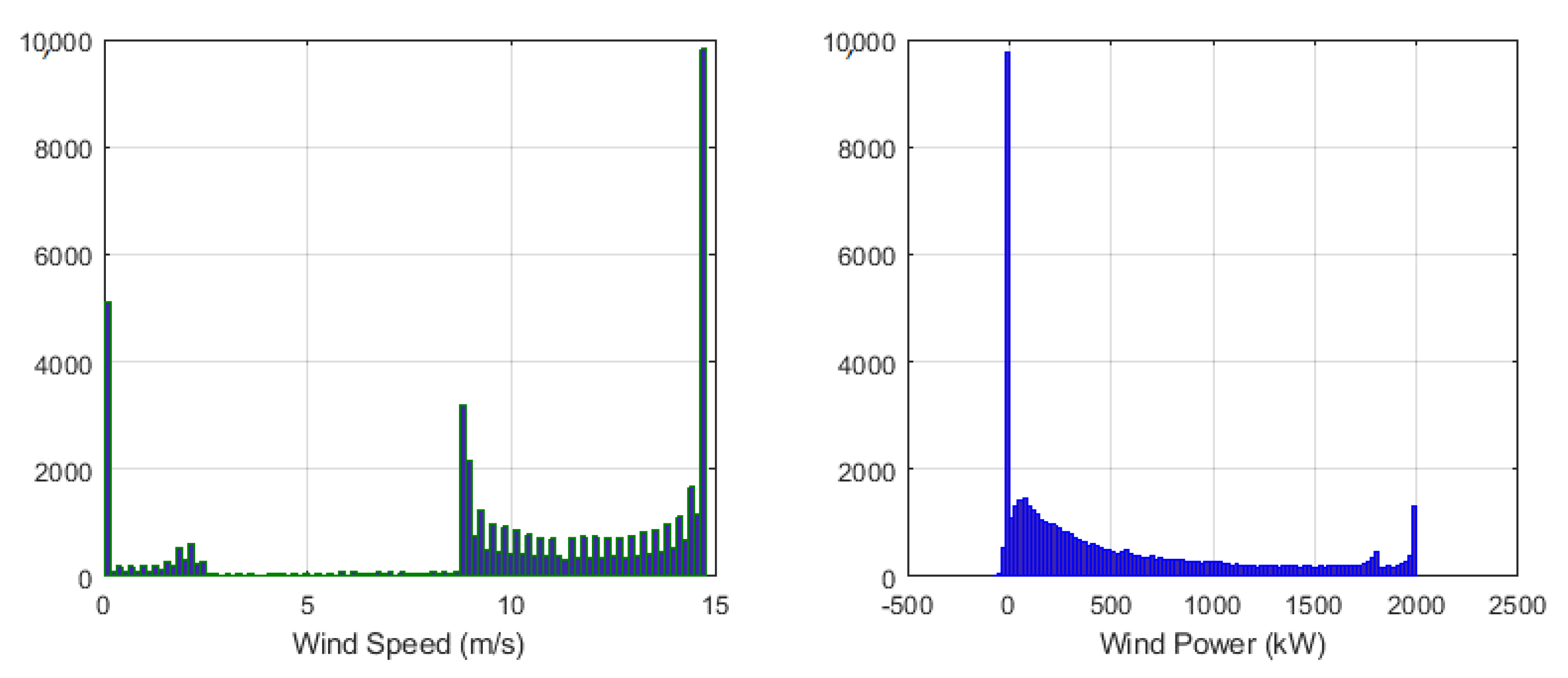
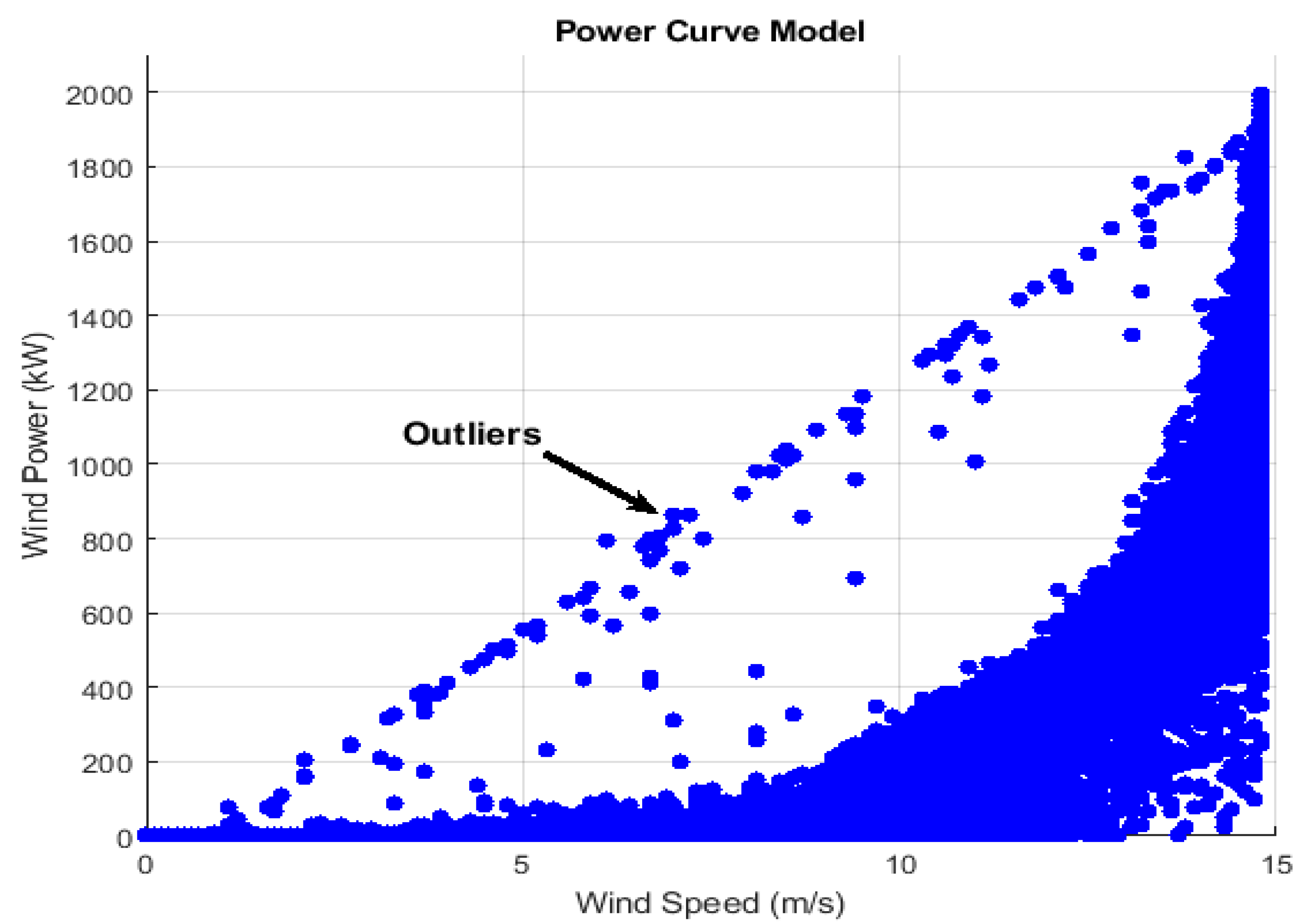
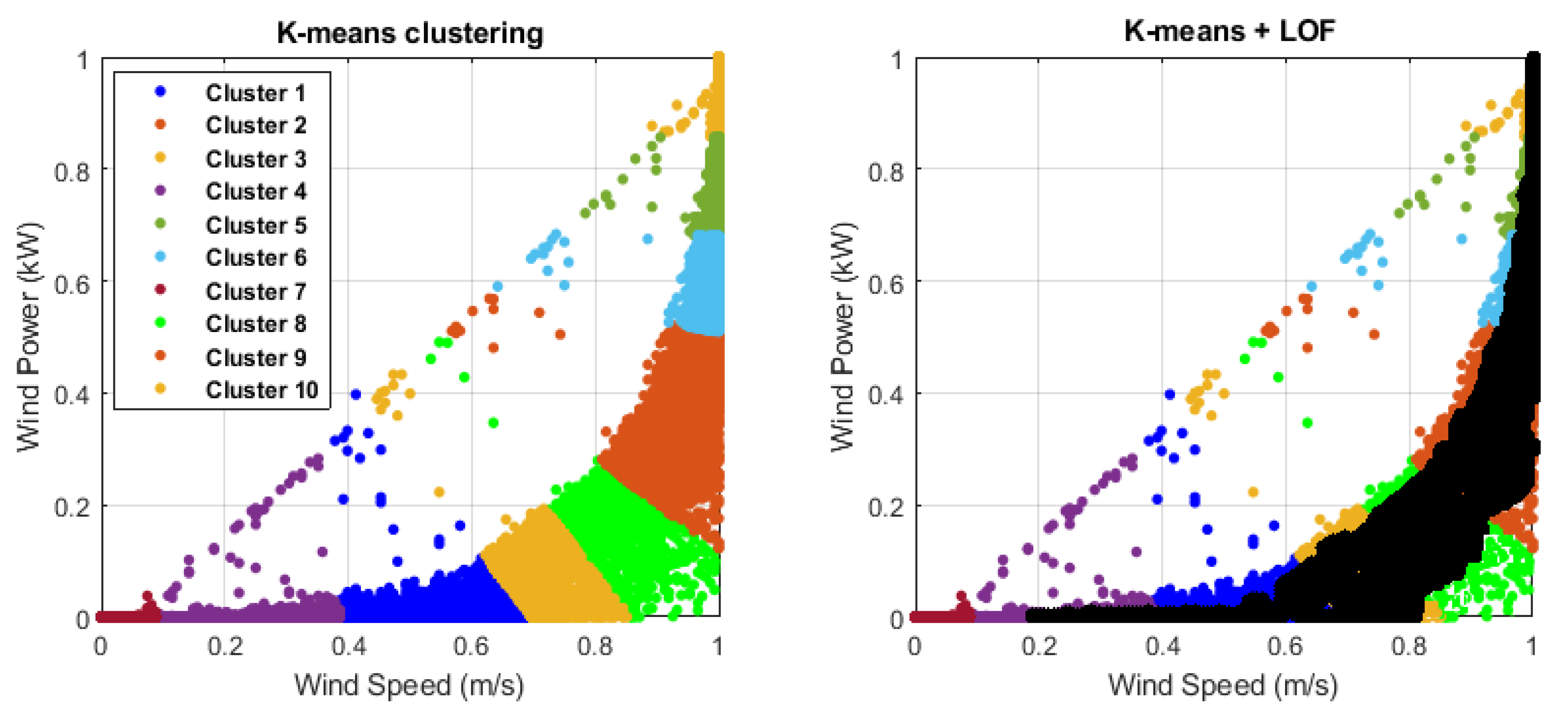
K-means is one of the most well-known clustering methods, a fast and efficient technique in unsupervised learning methods. However, it suffers from some deficiencies such as (i) predefining the number of clusters and centers in advance, (ii) not being able to handle noisy data and outliers properly, and finally, k-means is not proper to classify clusters with non-convex shapes. In order to deal with these listed issues, we proposed a combination of identifying density-based local outliers (LOF) and k-means for cleaning the raw supervisory control and data acquisition (SCADA) data as the initial section of the pre-processing.
(b)
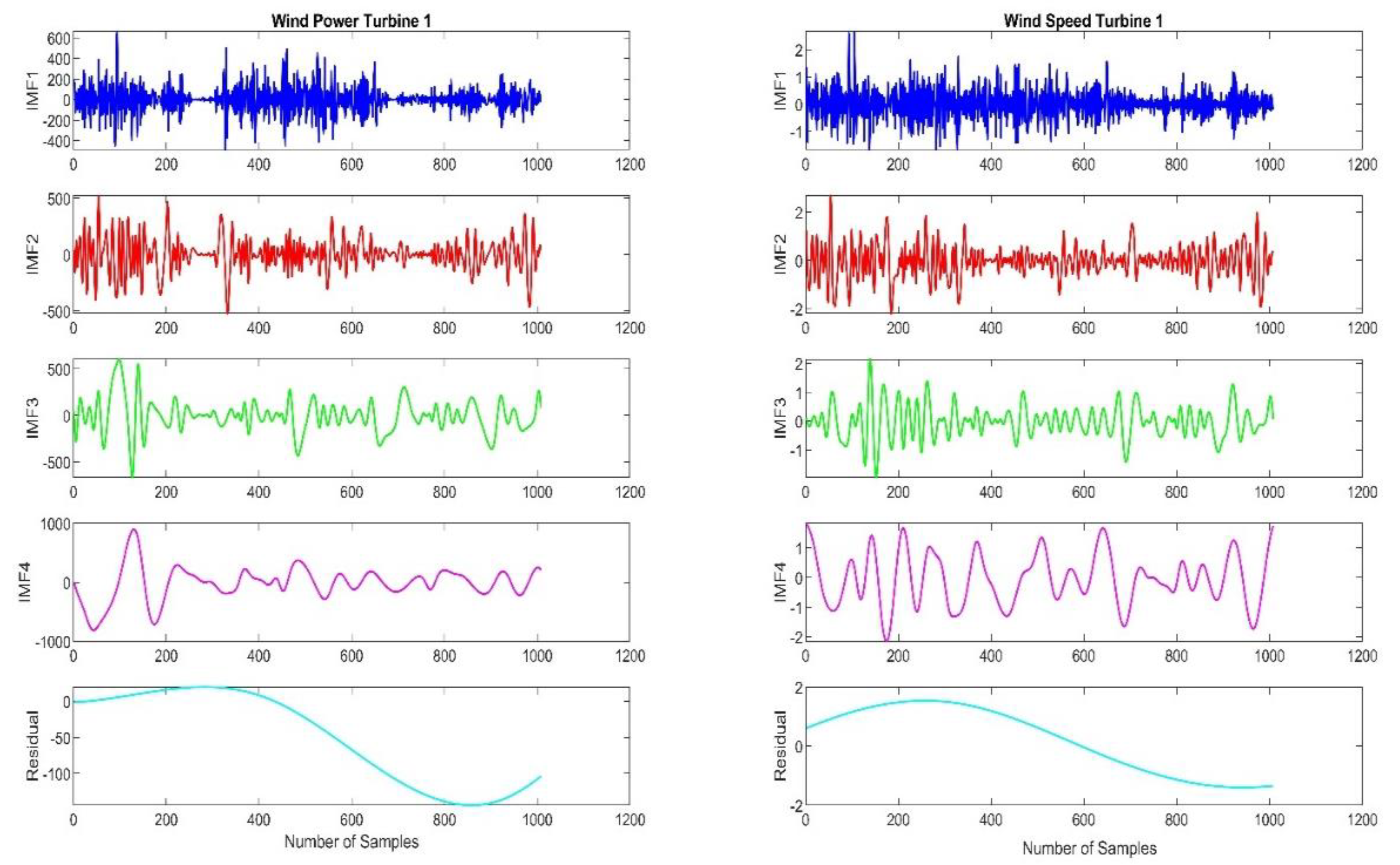
As wind speed and power forecasting involve the non-linear power curve, stochastic and noisy behavior of the recorded wind data, the empirical mode decomposition (EMD) method is proposed to deal with these uncertainties and increase the modelling accuracy.
(c)
Fuzzy-GMDH neural networks are considered as one of the most effective methods to model the time-series data with high-level noise and short input sampling. However, initializing the hyper-parameters of fuzzy-GMDH is challenging and time-consuming. With regards to adjusting the hyper-parameters, we apply a robust and fast search method called the grey wolf optimization (GWO) algorithm. Applying the GWO as a hyper-parameter tuner improved the proposed model’s accuracy and reliability to forecast wind power.
(d)
The proposed combined forecasting model has successfully verified on two actual wind turbines SCADA datasets. In addition, the proposed forecasting model is compared with the other valid combined forecasting models.

2. Materials and Methods

After a brief description of the SCADA system and data gathering, this section illustrates the artificial intelligence methods proposed in this paper.

2.1. SCADA System

The SCADA system, known as remote supervision and control of wind turbines in wind farms, plays a significant role in the wind power forecasting models. This paper’s collected and applied SCADA data is related to a large wind farm (located in Sweden). The input data includes the power output of wind turbines and wind speed (short-term with the interval of 10 min) for a year from Jan to Dec 2015. Furthermore, in order to evaluate and compare the performance of the proposed hybrid model, we applied the SCADA data for two wind turbines (wind turbine 1 (WT1) and wind turbine 2 (WT2)).

2.2. Proposed Wind Power Forecasting Strategy

In this study, a multi-step hybrid intelligent model has been proposed as a means to predict wind power production (see Figure 1).
Due to the wide range of intelligent methods such as neural networks and metaheuristic optimization algorithms, in this paper, we presented a hybrid forecasting model based on FGMDH and GWO for wind power production forecasting. The GWO optimization algorithm can perform the neural network (FGMDH) training step well and optimize the value of network parameters. Therefore, this algorithm (GWO) is constructive to the performance of the proposed model for predicting wind power production.
Since the structure of the input matrix plays a significant role in determining the output and accuracy of the model, in the first place, the various input signals (wind power and wind speed) are decomposed through the EMD method to different high and low frequencies (see Figure 2).
Five types of decomposed frequencies (IMF1, IMF2, IMF3, IMF4, residual) are selected and applied by delaying a unit of time (t-1) as inputs of the model subsequently (see Figure 3—inputs and output data structure). In addition, the lagged values (1 to 5) for the original wind power signal and actual wind speed signal are considered as input parameters (Figure 3—inputs and output data structure). In the next step, the FGMDH method has been employed to predict the wind turbine power.
The FGMDH model structure includes different neurons. The parameters grouped in the form of Gaussian variables and the weight of the fuzzy rule in each neuron are unknown. In this paper, the GWO algorithm is applied with the purpose of optimizing the FGMDH model variables (the group-unknown variables in neurons).
In this study, in order to evaluate the performance and reliability of forecasting models, the wind turbine power production is predicted for different seasons at two times (10-min and 1-h). The framework of the proposed model is represented in Figure 3.

2.3. Data Cleaning

The raw SCADA datasets usually include different forms of noise that directly negatively affect the accuracy of the forecasting process. One of the most notable outliers can be the negative wind turbine power outputs observed when the wind speed is shallow or during a failure situation. For evaluating the distribution of the raw SCADA dataset, Figure 1 is plotted, and also an abnormal distribution of wind power can be seen in Figure 4.
In the pre-processing section, it is recommended that [36] these negative powers should be set as zero. In addition, to remove the impact of the data scale, a Min-Max normalization is implemented for the feature scaling. Meanwhile, as each wind turbine has a unique power curve that presents the average efficiency of the applied wind turbine, without declaring the particular mechanical components, Figure 5 is plotted for showing this characteristic of the first wind turbine in this research. The scatter data point indicates the outliers.
The proposed cleaning data method is a combined K-means clustering and the identifying density-based local outliers (LOF) method [37]. In the first step, a k-means clustering method is employed to classify the SCADA data into various clusters. Then, in each cluster, the local density-based method is adopted to eliminate the potential noises. The clean data after using K-means clustering and the LOF method can be illustrated in Figure 6.

2.4. Empirical Mode Decomposition

The EMD is a method of signal decomposition that can analyse the non-linear and non-stationary time series. Moreover, using this method is more accessible and more understandable compared to wavelet decomposition [38,39]. In addition, EMD does not stand in the need of deciding a mother function in advance (beforehand of time) by no means such as wavelet decomposition. The most important characteristic of the EMD is a fully data-driven decomposing means by which signals break down into various independent components within the interval of local specifications of a signal.
Decomposing initial signals as intrinsic mode functions (IMFs) and residual into a finite amount of oscillatory functions is the concept of EMD. These IMFs must be met by the following conditions: (1) The number of extreme must be equal to the number of zero crossings or their maximum difference is equal to one; (2) the mean value of the envelopes characterized by local maxima and local minima must be zero at all components.
The EMD is a sifting method using a real signal to extract the IMFs and residual. The calculation of the EMD can be given as the following steps [38,39]:
Stage 1: Recognize all local maxima and local minima in time series S ( t ) .
Stage 2: Connect all local maxima and minima to produce the upper U(t) and lower L(t) envelopes using a cubic spline line.
Stage 3: Calculate the point-by-point mean envelope from the upper and lower envelopes and create the mean envelopes m ( t ) later as:
m ( t ) = [ U ( t ) + L ( t ) ] 2
Stage 4: Compute the distinction between the mean envelopes and the actual signal:
h ( t ) = S ( t ) m ( t )
Stage 5: Check whether h ( t ) is an intrinsic mode function (IMF). Provided that this is true, it is treated as the ith IMF and afterwards the actual time series is supplanted by the residuals h ( t ) = S ( t ) m ( t ) . If not, is supplanted by h ( t ) .
Stage 6: Repeat Steps 1–5 until the standard deviation magnitude of the two consecutive sifting results (IMFS and Residual) is lower than the predefined stopping criterion.
Using the above-mentioned sifting process, many IMFs can be obtained from high frequency to low frequency, thereby disintegrating into several IMFs and a residual as:
r n ( t ) = S ( t ) i = 1 n C i ( t )
where r n ( t ) and n are the last residuals and the number of IMFs, respectively. C i ( t ) ( i = 1 , 2 , , n ) indicates different IMFs.

2.5. Fuzzy-GMDH Model

The FGMDH is a machine learning strategy in the hierarchical structure [40]. In this model, every neuron has two inputs and an output. The general structure of the FGMDH system was shown in Figure 3 (the FGMDH forecasting model). In this figure, the output of each neuron in each layer is considered as the input in the following layer. The last output is determined to utilize the mean of the last layer output.
The FGMDH structure part in Figure 6 demonstrates that the inputs from the mth model and pth layer are the outputs of the (m − 1)th and mth model in the (p − 1)th layer. The numerical function for computing the y p m (the output variable of the mth model in the pth layer) is as follows:
y p m = f ( y p 1 , m 1 , y p 1 , m ) = k = 1 K μ k p m w k p m
μ k p m = exp { ( y p 1 , m 1 a k , 1 p m ) 2 b k , 1 p m ( y p 1 , m a k , 2 p m ) 2 b k , 2 p m }
where w k p m and μ k p m are its corresponding weight parameter and the kth Gaussian function, respectively. Moreover, a k p m and b k p m are the Gaussian parameters [41]. Furthermore, the last output is calculated by the following equation:
y = 1 M m = 1 M y p m
The learning procedure of feed forward FGMDH is known to solve the composite problems as an iterative technique.
A simplified fuzzy logic rule has been provided by [40] to improve the GMDH neural network:
If   x 1 = F k 1   and   x 2 = F k 2 ,   then   output   y = w k

2.6. Gray Wolf Optimization

The GWO algorithm, which is a new meta-heuristic algorithm based on swarm intelligence evolutionary, is proposed by Mirjalili et al. [42].
The GWO is inspired by grey wolves. The four types of grey wolves are hired as alpha, beta, delta, and omega to replicate the hierarchy of management. On the other side, the notable steps of grey wolves (encircling prey, hunting, attacking prey, and searching for prey) are performed during the operation [43].
Encircling prey: The encircling behaviour of each agent of the group is computed by the following mathematical formula:
d = | c . x p t x t |
x t + 1 = x p t a . d
The vectors a and c are computed as the following formula:
{ a = 2 l . r 1 c = 2 . r 2
Hunting: For a mathematical simulation of the hunting behaviour of grey wolves, it is assumed that α, β, and δ have better information about the possible location of the prey.
{ d α = | c 1 . x α x | d β = | c 2 . x β x | d δ = | c 3 . x δ x | , { d α = | c 1 . x α x | d β = | c 2 . x β x | d δ = | c 3 . x δ x |
x ( t + 1 ) = x 1 + x 2 + x 3 3
Attacking the prey and searching for the prey: The a is a random value in the interval [−2a, 2a]. When the random value is less than 1, the grey wolves are enforced to attack the prey and if the random value is greater than 1, the grey wolves are forced to diverge from the prey.

2.7. Error Indicators

In order to assess the accuracy and reliability of the proposed forecasting model, different error indicators have been used in this paper: The mean absolute percentage error (MAPE), the sum squared error (SSE), the root mean squared error (RMSE), and the mean absolute error (MAE). All error indicators are based on error percentage (unitless).
M A P E = 100 m i = 1 m | x r e a l i x f o r i x r e a l i |
S S E = i = 1 m ( x r e a l i x f o r i ) 2
R M S E = 1 m i = 1 m ( x r e a l i x f o r i ) 2
M A E = 1 m i = 1 m | x r e a l i x f o r i |
where x r e a l i and x f o r i are the actual value and predicted value, respectively. m is the number of data.

3. Results and Discussion

As discussed in the previous sections, in order to evaluate the performance and efficiency of the proposed method, the real on-shore SCADA dataset for two wind turbines (WT1 and WT2) has been exploited in this paper. Regarding the framework of the proposed model (Figure 3), several frequencies of wind speed (IMF1Speed, IMF2Speed, IMF3Speed, IMF4Speed, ResSpeed) and wind turbine power (IMF1Power, IMF2Power, IMF3Power, and IMF4Power, and ResPower) are considered as input parameters of the model:
O r i g i n a l   a n d   d e c o m p o s i t i o n   s i g n a l s { W P ( t 1 ) , W P ( t 2 ) , W P ( t 3 ) , W P ( t 4 ) , W P ( t 5 ) W S ( t 1 ) , W S ( t 2 ) , W S ( t 3 ) , W S ( t 4 ) , W S ( t 5 ) I M F 1 P o w e r ( t 1 ) ,   I M F 2 P o w e r ( t 1 ) ,   I M F 3 P o w e r ( t 1 ) , I M F 4 P o w e r ( t 1 ) ,   R e s P o w e r ( t 1 ) ,   I M F 1 S p e e d ( t 1 ) ,   I M F 2 S p e e d ( t 1 ) ,   I M F 3 S p e e d ( t 1 ) , I M F 4 S p e e d ( t 1 ) ,   R e s S p e e d ( t 1 )
In addition, several combined forecasting models such as MI-CNN [44], MRMR-HNES [45], MI-CNEA [46], GRNN, and FGMDH have been applied to measure the performance of the proposed model. First, the 1-year-dataset is selected as the prediction model data and the predicted results are calculated with the error indicators presented in the previous section. The results are shown in Table 1.
In Table 1, the prediction results are calculated for two wind turbines in two different time steps (10-min and 1-h). The wind turbine power production is highly dependent on the wind speed. On the other hand, the wind speeds vary greatly on different days thus, the forecasting time intervals for power production have been chosen amongst the days of the four following months: February, May, August, and November which have the highest fluctuation values for power production.
According to the results in Table 1, the performance of the proposed model is better than the other provided models in different time steps and wind turbines. In addition, the results indicate that the performance of the forecasting models in the 10-min time step is better than the 1-h time step. Table 2 and Figure 7 indicate the results of the proposed forecasting model and other models for wind turbine power production forecasting (WT1).
According to the results of Table 2 and Figure 7, the performance of the forecasting models has been evaluated in different time steps (10-min and 1-h) and seasons (winter, spring, summer, and fall). Based on these results, the proposed model can predict the wind turbine power more reliably and highly accurately multiple times ahead compared to the other valid forecasting models (GRNN, FGMDH, MI-CNN, MRMR-HNES, and MI-CNEA).

4. Conclusions

Considering the highly volatile and nonlinear process of wind turbines power production, a hybrid intelligent system to improve the accuracy and efficiency of wind turbine power prediction has been proposed. For the initial step, the hybrid K-means-LOF and EMD methods have been applied as a pre-processing step for removing the outliers and decomposition of the SCADA data, respectively. Then, the processed data was given to the forecasting model (FGMDH) and the future power of the wind turbine has been calculated. Furthermore, in order to complete the proposed model as a parallel calculation, the GWO algorithm has been used as an optimization method to optimize the FGMDH parameters. In this study, the SCADA data for two wind turbines in the real wind farm located in Sweden has been used to measure the performance and reliability of the proposed model.
The new forecasting model has been applied to predict the power of wind turbines for two time-intervals ahead (10-min and 1-h) in 1 year and different seasons. The obtained results pinpointed that the performance of the proposed method (EMD-FGMDH-GWO) at different time intervals has a high accuracy and reliability than many other available methods such as GRNN, FGMDH, MI-CNN, MRMR-HNES, and MI-CNEA. The MAPE error indicator obtained for GRNN, FGMDH, MI-CNN, MRMR-HNES, MI-CNEA and the proposed model is equal to 20.818, 11.883, 3.981, 5.105, 5.754, and 3.012, respectively. In addition, the proposed forecasting model can be extended and applied for different energy sources to maximize the use of renewable energy sources and better manage their use. In future studies, the proposed model will be extended to analyze different energy sources in one area simultaneously.

Author Contributions

Conceptualization, A.H.; data curation, A.H., M.M.N., and M.N.; investigation, A.H., M.M.N., and M.N.; methodology, A.H., M.N., and M.M.N.; validation, A.H., M.M.N., M.N., D.A.G., and F.K.; visualization, A.H., M.M.N., D.A.G., and F.K.; writing—original draft, A.H., D.A.G., F.K., and L.B.T.; writing—review and editing, A.H., D.A.G., F.K., and L.D.S.; supervision, D.A.G., F.K., L.D.S., and L.B.T. All authors have read and agreed to the published version of the manuscript.

Funding

This research received no external funding.

Institutional Review Board Statement

Not applicable.

Informed Consent Statement

Not applicable.

Conflicts of Interest

The authors declare no conflict of interest.

References

  1. Okumus, I.; Dinler, A. Current status of wind energy forecasting and a hybrid method for hourly predictions. Energy Convers. Manag. 2016, 123, 362–371. [Google Scholar] [CrossRef]
  2. Zhao, Y.; Ye, L.; Li, Z.; Song, X.; Lang, Y.; Su, J. A novel bidirectional mechanism based on time series model for wind power forecasting. Appl. Energy 2016, 177, 793–803. [Google Scholar] [CrossRef]
  3. Karki, R.; Hu, P.; Billinton, R. A simplified wind power generation model for reliability evaluation. IEEE Trans. Energy Convers. 2006, 21, 533–540. [Google Scholar] [CrossRef]
  4. Li, S.; Wunsch, D.C.; O’Hair, E.A.; Giesselmann, M.G. Using neural networks to estimate wind turbine power generation. IEEE Trans. Energy Convers. 2001, 16, 276–282. [Google Scholar] [CrossRef]
  5. Xia, S.; Chan, K.W.; Luo, X.; Bu, S.; Ding, Z.; Zhou, B. Optimal sizing of energy storage system and its cost-benefit analysis for power grid planning with intermittent wind generation. Renew. Energy 2018, 122, 472–486. [Google Scholar] [CrossRef]
  6. Akçay, H.; Filik, T. Short-term wind speed forecasting by spectral analysis from long-term observations with missing values. Appl. Energy 2017, 191, 653–662. [Google Scholar] [CrossRef]
  7. Toh, G.K.; Gooi, H.B. Incorporating forecast uncertainties into EENS for wind turbine studies. Electr. Power Syst. Res. 2011, 81, 430–439. [Google Scholar] [CrossRef]
  8. Ortega-Vazquez, M.A.; Kirschen, D.S. Estimating the spinning reserve requirements in systems with significant wind power generation penetration. IEEE Trans. Power Syst. 2009, 24, 114–124. [Google Scholar] [CrossRef]
  9. Wu, J.; Zhang, B.; Li, H.; Li, Z.; Chen, Y.; Miao, X. Statistical distribution for wind power forecast error and its application to determine optimal size of energy storage system. Int. J. Electr. Power Energy Syst. 2014, 55, 100–107. [Google Scholar] [CrossRef]
  10. Usaola, J. Probabilistic load flow with correlated wind power injections. Electr. Power Syst. Res. 2010, 80, 528–536. [Google Scholar] [CrossRef]
  11. Balasubramaniam, K.; Saraf, P.; Hadidi, R.; Makram, E.B. Energy management system for enhanced resiliency of microgrids during islanded operation. Electr. Power Syst. Res. 2016, 137, 133–141. [Google Scholar] [CrossRef]
  12. Bruninx, K.; Delarue, E. A statistical description of the error on wind power forecasts for probabilistic reserve sizing. IEEE Trans. Sustain. Energy 2014, 5, 995–1002. [Google Scholar] [CrossRef]
  13. Zhang, Z.S.; Sun, Y.Z.; Gao, D.W.; Lin, J.; Cheng, L. A versatile probability distribution model for wind power forecast errors and its application in economic dispatch. IEEE Trans. Power Syst. 2013, 28, 3114–3125. [Google Scholar] [CrossRef]
  14. Tascikaraoglu, A.; Sanandaji, B.M.; Chicco, G.; Cocina, V.; Spertino, F.; Erdinc, O.; Paterakis, N.G.; Catalao, J.P. A short-term spatio-temporal approach for Photovoltaic power forecasting. In Proceedings of the 2016 Power Systems Computation Conference (PSCC), Genoa, Italy, 20–24 June 2016. [Google Scholar] [CrossRef]
  15. Li, S.; Dong, W.; Huang, J.; Wu, Z.; Zhang, H. Wind power system reliability sensitivity analysis by considering forecast error based on non-standard third-order polynomial normal transformation method. Electr. Power Syst. Res. 2019, 167, 122–129. [Google Scholar] [CrossRef]
  16. Heydari, A.; Astiaso Garcia, D.; Keynia, F.; Bisegna, F.; De Santoli, L. A novel composite neural network based method for wind and solar power forecasting in microgrids. Appl. Energy 2019, 251, 113353. [Google Scholar] [CrossRef]
  17. Cui, Y.; Bangalore, P.; Bertling Tjernberg, L. An Anomaly Detection Approach Based on Machine Learning and SCADA Data for Condition Monitoring of Wind Turbines. In Proceedings of the 2018 IEEE International Conference on Probabilistic Methods Applied to Power Systems (PMAPS), Boise, ID, USA, 24–28 June 2018; pp. 1–6. [Google Scholar]
  18. Heydari, A.; Keynia, F. A new intelligent heuristic combined method for short-term electricity price forecasting in deregulated markets. Aust. J. Electr. Electron. Eng. 2016, 13, 258–267. [Google Scholar] [CrossRef]
  19. Zhang, X.; Wang, J.; Zhang, K. Short-term electric load forecasting based on singular spectrum analysis and support vector machine optimized by Cuckoo search algorithm. Electr. Power Syst. Res. 2017, 146, 270–285. [Google Scholar] [CrossRef]
  20. Kouhi, S.; Keynia, F.; Najafi Ravadanegh, S. A new short-term load forecast method based on neuro-evolutionary algorithm and chaotic feature selection. Int. J. Electr. Power Energy Syst. 2014, 62, 862–867. [Google Scholar] [CrossRef]
  21. Amjady, N.; Keynia, F.; Zareipour, H. Short-term wind power forecasting using ridgelet neural network. Electr. Power Syst. Res. 2011, 81, 2099–2107. [Google Scholar] [CrossRef]
  22. Han, Q.; Meng, F.; Hu, T.; Chu, F. Non-parametric hybrid models for wind speed forecasting. Energy Convers. Manag. 2017, 148, 554–568. [Google Scholar] [CrossRef]
  23. Pelajo, J.C.; Brandão, L.E.T.; Gomes, L.L.; Klotzle, M.C. Wind farm generation forecast and optimal maintenance schedule model. Wind Energy 2019, 22, 1872–1890. [Google Scholar] [CrossRef]
  24. Osório, G.J.O.; Matias, J.C.O.; Catalão, J.P.S. Hybrid evolutionary-adaptive approach to predict electricity prices and wind power in the short-term. In Proceedings of the 2014 Power Systems Computation Conference, Wroclaw, Poland, 18–22 August 2014. [Google Scholar] [CrossRef]
  25. Gallego-Castillo, C.; Cuerva-Tejero, A.; Bessa, R.J.; Cavalcante, L. Wind power probabilistic forecast in the reproducing kernel Hilbert space. In Proceedings of the 2016 Power Systems Computation Conference (PSCC), Genoa, Italy, 11 August 2016; pp. 1–7. [Google Scholar] [CrossRef] [Green Version]
  26. Xiao, L.; Shao, W.; Yu, M.; Ma, J.; Jin, C. Research and application of a hybrid wavelet neural network model with the improved cuckoo search algorithm for electrical power system forecasting. Appl. Energy 2017, 198, 203–222. [Google Scholar] [CrossRef]
  27. Shi, K.; Qiao, Y.; Zhao, W.; Wang, Q.; Liu, M.; Lu, Z. An improved random forest model of short-term wind-power forecasting to enhance accuracy, efficiency, and robustness. Wind Energy 2018, 21, 1383–1394. [Google Scholar] [CrossRef]
  28. Doan, V.Q.; Kusaka, H.; Matsueda, M.; Ikeda, R. Application of mesoscale ensemble forecast method for prediction of wind speed ramps. Wind Energy 2019, 22, 499–508. [Google Scholar] [CrossRef]
  29. Duan, J.; Wang, P.; Ma, W.; Tian, X.; Fang, S.; Cheng, Y. Short-term wind power forecasting using the hybrid model of improved variational mode decomposition and Correntropy Long Short -term memory neural network. Energy 2021, 214, 118980. [Google Scholar] [CrossRef]
  30. Yildiz, C.; Acikgoz, H.; Korkmaz, D.; Budak, U. An improved residual-based convolutional neural network for very short-term wind power forecasting. Energy Convers. Manag. 2021, 228, 113731. [Google Scholar] [CrossRef]
  31. Jafarzadeh, S.; Manjili, S.; Mardani, A.; Kamali, M. An extended new approach for forecasting short-term wind power using modified fuzzy wavelet neural network: A case study in wind power plant. Energy 2021, 223, 120052. [Google Scholar] [CrossRef]
  32. Groppi, D.; De Santoli, L.; Cumo, F.; Astiaso Garcia, D. A GIS-based model to assess buildings energy consumption and usable solar energy potential in urban areas. Sustain. Cities Soc. 2018, 40, 546–558. [Google Scholar] [CrossRef]
  33. De Santoli, L.; Mancini, F.; Astiaso Garcia, D. A GIS-based model to assess electric energy consumptions and usable renewable energy potential in Lazio region at municipality scale. Sustain. Cities Soc. 2019, 46, 101413. [Google Scholar] [CrossRef] [Green Version]
  34. Mancini, F.; Nastasi, B. Solar energy data analytics: PV deployment and land use. Energies 2020, 13, 417. [Google Scholar] [CrossRef] [Green Version]
  35. Nastasi, B.; De Santoli, L.; Albo, A.; Bruschi, D.; Lo Basso, G. RES (Renewable Energy Sources ) availability assessments for Eco- fuels production at local scale: Carbon avoidance costs associated to a hybrid biomass/H 2 NG-based energy scenario. Energy Procedia 2015, 81, 1069–1076. [Google Scholar] [CrossRef] [Green Version]
  36. Huang, Q.; Cui, Y.; Bertling Tjernberg, L.; Bangalore, P. Wind turbine health assessment framework based on power analysis using machine learning method. In Proceedings of the 2019 IEEE PES Innovative Smart Grid Technologies Europe (ISGT-Europe), Bucharest, Romania, 29 September–2 October 2019; pp. 1–5. [Google Scholar] [CrossRef]
  37. Breuniq, M.M.; Kriegel, H.P.; Ng, R.T.; Sander, J. LOF: Identifying density-based local outliers. SIGMOD Rec. (ACM Spec. Interes. Gr. Manag. Data) 2000, 29, 93–104. [Google Scholar] [CrossRef]
  38. Huang, N.E.; Shen, Z.; Long, S.R.; Wu, M.C.; Shih, H.H.; Zheng, Q.; Yen, N.C.; Tung, C.C.; Liu, H.H. The empirical mode decomposition and the Hilbert spectrum for nonlinear and non-stationary time series analysis. Proc. R. Soc. Lond. Ser. A Math. Phys. Eng. Sci. 1998, 454, 903–995. [Google Scholar] [CrossRef]
  39. Huang, N.E.; Wu, M.L.; Qu, W.; Long, S.R.; Shen, S.S.P. Applications of Hilbert-Huang transform to non-stationary financial time series analysis. Appl. Stoch. Model. Bus. Ind. 2003, 19, 245–268. [Google Scholar] [CrossRef]
  40. Ohtani, T.; Ichihashi, H.; Miyoshi, T.; Nagasaka, K. Orthogonal and successive projection methods for the learning of neurofuzzy GMDH. Inf. Sci. 1998, 110, 5–24. [Google Scholar] [CrossRef]
  41. Najafzadeh, M. Neurofuzzy-based GMDH-PSO to predict maximum scour depth at equilibrium at culvert outlets. J. Pipeline Syst. Eng. Pr. 2016, 7, 06015001. [Google Scholar] [CrossRef]
  42. Mirjalili, S.; Mirjalili, S.M.; Lewis, A. Grey Wolf Optimizer. Adv. Eng. Softw. 2014, 69, 46–61. [Google Scholar] [CrossRef] [Green Version]
  43. Song, J.; Wang, J.; Lu, H. A novel combined model based on advanced optimization algorithm for short-term wind speed forecasting. Appl. Energy 2018, 215, 643–658. [Google Scholar] [CrossRef]
  44. Keynia, F. A new feature selection algorithm and composite neural network for electricity price forecasting. Eng. Appl. Artif. Intell. 2012, 25, 1687–1697. [Google Scholar] [CrossRef]
  45. Amjady, N.; Keynia, F. Application of a new hybrid neuro-evolutionary system for day-ahead price forecasting of electricity markets. Appl. Soft Comput. 2010, 10, 784–792. [Google Scholar] [CrossRef]
  46. Amjady, N.; Keynia, F. Day ahead price forecasting of electricity markets by a mixed data model and hybrid forecast method. Int. J. Electr. Power Energy Syst. 2008, 30, 533–546. [Google Scholar] [CrossRef]
Figure 1. General schematic of the proposed forecasting model.
Energies 14 03459 g001
Figure 2. The EMD output, i.e., decomposition signals of wind power and wind speed of turbine 1 (WT1).
Energies 14 03459 g002
Figure 3. The framework of the proposed model.
Energies 14 03459 g003
Figure 4. The distribution of the raw SCADA data WT1 (wind speed and power).
Energies 14 03459 g004
Figure 5. The power curve model of the WT1.
Energies 14 03459 g005
Figure 6. The K-means clustering method performance and the applied data (WT1) divided into 10 clusters (left). The dark points represent the clean SCADA data after applying the LOF (right).
Energies 14 03459 g006
Figure 7. The wind turbine power forecasting results of the comparative models for WT1.
Energies 14 03459 g007
Table 1. Comparison of the wind turbine power forecasting errors of the models for two wind turbines (WT1 and WT2).
Forecasting ModelsTime StepError Criteria
RMSESSEMAEMAPE
WT1WT2WT1WT2WT1WT2WT1WT2
GRNN10-min0.3150.29125.011102.290.2990.26518.51620.818
1-h0.3810.387133.366124.9710.3120.36521.81522.716
FGMDH10-min0.2360.24118.53319.0840.2170.2289.23211.883
1-h0.2880.27264.26554.0790.2760.23110.23712.11
MI-CNN [44]10-min0.0560.07213.3512.8160.0450.0334.2623.981
1-h0.0940.08540.5841.7320.0680.0384.8375.002
MRMR-HNES [45]10-min0.1490.18411.9229.8180.1430.1664.5235.105
1-h0.1670.20244.51451.1650.1490.1715.5925.235
MI-CNEA [46]10-min0.2250.21914.36813.1270.2150.1876.8155.754
1-h0.2530.22653.12256.4640.2240.2036.947.402
Proposed Model10-min0.0130.01310.7068.0690.0120.012.8563.012
1-h0.0260.02436.59434.0790.0320.0123.2083.516
Table 2. Comparison of the wind turbine power forecasting errors of the models for the different seasons of a year.
Different SeasonsError CriteriaGRNNFGMDHMI CNN [44]MRMR HNES [45]MI CNEA [46]Proposed Model
1-h10-min1-h10-min1-h10-min1-h10-min1-h10-min1-h10-min
WinterRMSE0.4820.4140.3260.3180.1220.0830.1730.1530.2620.2260.0150.013
SSE171.31546.55537.33616.26519.8209.35228.81911.47422.87213.07717.6346.317
MAE0.4450.3960.3060.2770.0790.0490.1470.1440.2290.2240.0130.012
MAPE22.45823.57212.5369.8445.3154.7476.9394.47810.3926.7483.9372.504
SpringRMSE0.3830.4010.3090.2980.1100.0860.1630.1470.2440.2320.0140.012
SSE131.71951.51340.54615.32719.6087.34233.54911.49328.09014.12011.5195.306
MAE0.3630.3590.2840.2750.0740.0540.1470.1380.2220.2080.0190.012
MAPE20.44519.81915.04911.8185.3694.9537.2584.74610.8497.1534.1252.263
SummerRMSE0.3410.3130.3020.2910.0810.0640.1690.1430.2530.2460.0140.012
SSE121.48137.91441.15113.01112.7805.31113.9077.45328.99412.03011.1343.006
MAE0.3130.2640.2740.2880.0550.0400.1480.1430.2230.2160.0170.012
MAPE21.51616.60715.47913.4546.3494.3488.5834.9449.8107.4504.0193.917
FallRMSE0.3720.3280.2850.2680.1180.0740.1630.1620.2470.2440.0180.014
SSE91.81934.72553.18326.13022.3789.42724.23810.58737.39018.33713.2386.263
MAE0.4150.3070.2390.2340.0800.0400.1610.1370.2430.2070.0150.014
MAPE24.16018.50418.71011.3667.4193.4988.1414.11910.4876.2143.0152.903
Publisher’s Note: MDPI stays neutral with regard to jurisdictional claims in published maps and institutional affiliations.

