
The Impact of the COVID-19 Pandemic on Gaseous and Solid Air Pollutants Concentrations and Emissions in the EU, with Particular Emphasis on Poland


1
Department of Electrical Engineering and Industrial Automation, Faculty of Mining, Safety Engineering and Industrial Automation, Silesian University of Technology, 44-100 Gliwice, Poland
2
Department of Physical Chemistry and Technology of Polymers, Faculty of Chemistry, Silesian University of Technology, 44-100 Gliwice, Poland
*
Author to whom correspondence should be addressed.
Energies 2021, 14(11), 3264; https://doi.org/10.3390/en14113264
Submission received: 12 April 2021
/
Revised: 25 May 2021
/
Accepted: 28 May 2021
/
Published: 2 June 2021
(This article belongs to the Special Issue The Effects of COVID-19 on Renewable Energy Supply, Demand and Energy Mix)
Abstract
:This article presents the research on the analysis of the impact of social isolation caused by the COVID-19 pandemic on gaseous air pollutant concentrations. For this purpose, the authors presented (thermal maps) and analyzed the concentrations of selected gases such as NO2, CO, SO2, and PM2.5 particles during the strict quarantine period in Poland and other EU countries. Statistical analysis of the concentration level of these gases was performed. It was noticed that in Poland, Germany, and France, the concentrations of such gases as CO, NO2, and PM2.5 particles decreased, while in Italy and Spain, the tendency was the opposite. To verify whether the discovered dependencies are not a natural continuation of the trends shaping the given phenomenon, the time series of gas and PM2.5 particle emissions were analyzed. On this basis, the emission forecast up to 2023 was created, using the ARIMA class models. The obtained results allowed to construct five scenarios for the development of NO2, CO, SO2, and PM2.5 emissions until 2023, considering the impact of the COVID-19 pandemic. It was stated that in the optimistic scenario, in 2023, a decrease in CO, NO2, and PM2.5 emissions could be achieved by maximums of 51%, 95%, and 28%, respectively.
1. Introduction
The article presents the impact of the COVID-19 pandemic on the level of gaseous and solid air pollutants concentrations in Poland compared to selected European Union countries. Gaseous and solid air pollutants emissions lead to hardly reversible global climate effects. They are influenced by the change in the temperature of the planet, caused mainly by the combustion of fossil fuels in energy, transport, and industry. Therefore, the aim of the article was to demonstrate the impact of changes in the lifestyle of European Union citizens, forced by the restrictions related to the pandemic, on the level of gaseous and solid air pollutants emissions. Similar studies related to the impact of the effects of COVID-19 on air pollutant emissions have been conducted by many researchers around the world [1,2,3,4,5,6,7,8]. However, such studies have not been conducted in the case of Poland and do not include the creation of scenarios considering a COVID-19 lockdown factor. Such scenarios will provide an insight into the evolution of air pollutant emissions in the coming years.
The first confirmed case of COVID-19 in Poland was announced on 4 March 2020, and the state of epidemic threat was introduced on 14 March 2020. Poland was one of the few countries that introduced a lockdown at the very beginning of the pandemic when there were only six cases and no deaths had yet been recorded [9]. On 10–25 March 2020, universities, secondary and primary schools were closed (6 days after the first case), mass events were abandoned, sanitary checks at the borders were introduced, and restrictions on social contacts were implemented. As a result, during the first wave of the pandemic, it was possible to avoid a rapid increase in the incidence of the disease and prepare the country for the need to provide adequate medical care to its inhabitants.
For comparison, in Italy, a country in which the pandemic development pace was one of the fastest, the first case of COVID-19 was recorded in January, and the first restrictions on interpersonal contacts were introduced only in mid-March. During this time, about 4000 cases of illnesses and over 300 deaths were registered daily. In the analyzed period, the number of cases of illness and death in Poland and Italy was also analyzed. It was noted that deaths in Poland amounted to 4%, and disease cases to 12%.
The implemented safety measures resulted in the limitation of air, road, and rail traffic [10,11]. The level of production in many enterprises was also reduced, and thus the pace of economic development [12]. The conducted analysis made it possible to study the impact of the COVID-19 pandemic, and thus the traffic and industrial activity, on the natural environment. Before the pandemic, it was assumed that in 2020, the amount of gas emissions would not be reduced.
This article presents the analysis of the impact of social isolation caused by the COVID-19 pandemic on selected gaseous air pollutant concentrations (NO2, CO, SO2), and PM2.5 particles. The paper examines this issue in relation to Poland, but also to selected European Union countries that were most affected by the COVID-19 action. They are Germany, France, Spain, and Italy. The research covered the period of strict quarantine in Poland, i.e., the period from 20 March to 15 April 2020. To verify whether the discovered dependencies are not a natural continuation of the trends shaping the given phenomenon, the time series of gas and PM2.5 particles emissions were analyzed. From these time series, the emission forecast up to 2023 was created, using ARIMA class models. The obtained results allowed to construct five scenarios for the development of NO2, CO, SO2, and PM2.5 emissions until 2023, considering the impact of the COVID-19 pandemic.
The impact of quarantine on gas and PM2.5 emissions was investigated by the authors. Heat maps showing the concentration levels of the tested substances during the lockdown and mathematical models to forecast changes in gas emissions until 2023 due to the outbreak of the pandemic were built by the authors. Such a phenomenon has not appeared in Europe for over 100 years. Therefore, the authors decided to build emission scenarios for selected air pollutants. Scenario planning is used precisely in cases when it is necessary to predict the influence of unexpected and previously unknown factors on the analyzed phenomenon. Undoubtedly, social isolation associated with COVID-19 is such a factor. When building the scenarios, the authors used mathematical models to eliminate the drawbacks of the scenarios created with the use of heuristic methods. This makes the scenarios more plausible because their assumptions are based on the results of empirical data analyses and mathematical models, and not only the subjective opinions of experts. The article presents a comprehensive analysis of air pollutants that adversely affect the health of the society. It is of particular importance in the case of Poland, where environmental pollution is the main problem of our time.
2. Materials and Methods
The authors focused on two terms related to air quality: concentration and emission. Such a procedure was used because of the short lockdown duration. Contrary to emissions, the concentration additionally considers the conditions in the place where the air pollution test was conducted, i.e., the topography, and buildings. The research was conducted in large cities—capitals (especially in Warsaw). For example, the walls of buildings form so-called urban street canyons, which means that the same number of cars causes a greater concentration of pollution in the city than on the highway, for example. This was what mattered during the lockdown period when city traffic was severely restricted. On the other hand, emission makes it possible to analyze the pollutants per unit of time in the case of the carried-out research per year.
In this article, gases such as carbon monoxide, nitrogen dioxide, sulfur dioxide, and PM2.5 particulate matter were analyzed simultaneously.
The procedure for conducting the presented analysis was as follows:
- The concentrations of selected gases, such as NO2, CO, SO2, and PM2.5 particles, during the period of strict quarantine in Poland, which took place on 20 March to 15 April 2020, were analyzed. The obtained concentration values of these substances were compared to the base year, which was 2018. The choice of 2018 was made deliberately. At the time of the research, the data for 2019 were still incomplete, and the choice of a more distant year could not be reliable.
- Based on data on the concentration levels of selected substances, heat maps of emissions in the studied period were created. The data presented in this way are much clearer and it is possible to easily detect trends by visual analysis.
- Changes in the emission levels of selected gaseous and solid air pollutants in 2018–2020 were examined and statistical analysis of the emission level was performed.
- Forecasts of gaseous and solid air pollutants emissions until 2023 were created. To verify whether the discovered relationships are not a natural continuation of the trends shaping a given phenomenon, the time series of gas and PM2.5 particles emissions were analyzed and then a forecast of emissions until 2023 was created on their basis.
- The obtained results made it possible to construct scenarios for NO2, CO, SO2, and PM2.5 emissions until 2023, considering the impact of the COVID-19 pandemic. Gaseous and solid air pollutants emissions up to 2023 were simulated in five scenarios.
To carry out the presented analysis, the methods described below were used.
2.1. Database Description
The analyzed data were obtained from the Copernicus Atmosphere Monitoring Service (CAMS), European Environment Agency, Eurostat, European Centre for Disease Prevention and Control and the Chief Inspectorate for Environmental Protection. The data for 2020 at five-day intervals were compared with the data for 2018. Additionally, the selected substances were analyzed and forecasted until 2023. ARIMA models were used for this purpose [13,14,15].
Table 1 shows which data and sources were used in a specific analysis. The data units are also presented in the table. The figures and tables present the results of the analyses carried out by the authors.
2.2. Forecasting Methods
ARIMA models were used to build mathematical models characterizing NO2, CO, SO2, and PM2.5 particles emissions. The created models made it possible to determine the emission forecasts of the above-mentioned substances until 2023. This, in turn, allowed to determine the trend of further development of the analyzed phenomenon. The obtained forecasts also became the basis for scenario planning, the results of which are presented in the article. Models were created using the univariate time series analysis Gretl 2018a software tool. The software was developed at Wake Forest University in the United States, NC.
The AR process model is described by the following equation:
where:
t, t − 1, …, t − p—time periods,
—lag,
—parameters of the model,
—white noise,
—value of the forecasted variable in a moment of time or during a period.
In the case of the MA model, the forecast was based on past observations and the differences between the past values and the forecast values (for the rest of the model). The model describes the following relationship:
where:
—the residuals of the model in periods t, t − 1, …, t − q.
q—time lag.
ARIMA (autoregressive integrated moving average) is a group of models used to describe stochastic processes. They consist of AR processes, i.e., autoregressive and MA (moving average) moving average processes. In the case of the AR (autoregression) process, the current series value is the sum of the linear combination of the previous series observations as well as the random disturbance [16,17].
Data on CO, NO2, SO2, and PM2.5 emissions were used during the estimation. The data concerned the average emission in Poland in the years 2006–2018. A Kalman filter was also introduced.
The default estimation method for ARIMA models is the exact maximum likelihood estimation using the Kalman filter. The Kalman filter provides a very efficient and accurate way to compute the likelihood of ARIMA models. The maximum likelihood estimation determines values for the following model parameters [18]:
where:
—state vector,
yt—vector of observables,
—variance matrix,
. —known square transition matrix of the process,
—rectangular measurement matrix,
—vector of exogenous variables,
vt, —vector white noise.
The models presented in the article were those that had the best parameters among the built models. During the selection, factors such as ex-post forecast error, characteristics of model residuals, their distribution, and autocorrelation [19,20] were considered. The information criteria were also taken into account [21].
2.3. Scenario Planning
Scenarios are a useful planning tool in an uncertain and complex environment. In this case, they facilitate making decisions, the consequences of which will be felt for a long time. It is also a case of forecasting the emission of gaseous and solid air pollutants. Scenario planning is a disciplined method for imagining possible futures that companies have applied to a great range of issues [22]. The scenarios present more than one vision of the future, indicating what could potentially happen. The scenarios are not intended to accurately predict the future, but only indicate and inform the recipients of the scenarios about possible future states of the analyzed phenomenon. The scenarios presented in the article are based on the created forecasts. The impact of the COVID-19 pandemic on the projected CO, NO2, and PM2.5 emissions by 2023 was simulated. The simulation was not performed for sulfur dioxide due to the already decreasing trend characterizing this time series. Five scenarios for the development of individual gases and PM2.5 emissions were created. These are the scenarios as follows:
- Forecast (scenario m, l): The most probable scenario, which is the emission forecast;
- Scenario o: The optimistic scenario obtained based on the 95% confidence interval of the forecast, constituting the lower limit of the range within which the forecast value may move to 95% probability;
- Scenario p: The pessimistic scenario obtained based on the 95% confidence interval of the forecast, constituting the upper limit of the range within which the forecast value may move with 95% probability;
- COVID-19 effect (scenario o): Optimistic scenario considering the impact of quarantine on the emission level in the analyzed period. From the calculated changes for the adopted days, the lowest percentage decrease in the emission of harmful substances was assumed. In the optimistic scenario, it was assumed that the emission decreased by this designated value in relation to the previous year;
- COVID-19 effect (scenario p): Pessimistic scenario considering the impact of quarantine on the level of emissions in the period 20 March to 15 April 2020. From the calculated changes for the adopted days, the lowest percentage decrease in the emission of harmful substances was assumed. In turn, in the pessimistic scenario, it was assumed that the emission decreased by this determined value in relation to the obtained emission forecast.
The scenarios were created in the following steps:
- (a)
- Entering data into the ARIMA model;
- (b)
- Choosing the optimal model with appropriate parameters;
- (c)
- Creation of a forecast based on the selected ARIMA model until 2023 (scenarios m, l),
- (d)
- Construction of the confidence interval (scenarios o, p);
- (e)
- Analysis of the impact of lockdown on changes in the emission level of tested substances, determination of the maximum and minimum decrease in emissions;
- (f)
- Recalculation of the forecast from step c, considering the abovementioned decrease in emissions (COVID-19 effect scenarios).
The confidence interval estimation is based on the construction of a numerical interval with a predetermined probability, which contains the unknown, true value of the estimated parameter. The interval sought is called the confidence interval, and the probability is denoted as (1 − α). In the presented studies, α is 95%. Alpha, i.e., the level of significance, means the probability of making an acceptable error. This was assumed to be 5%. Confidence intervals were estimated using the Barrodale–Roberts method [18].
2.4. Spatial Analysis
To make the research presented in the article possible, the spatial information system QGIS version 3.10.2 was used. The QGIS project is part of the Open Source Geospatial Foundation (OSGeo). Spatial information systems are a powerful set of tools for the collection, storage, free recovery, processing, and presentation of real-world spatial data [23,24,25].
GIS provided tools, such as geocoding and the creation of heat maps. Geocoding is the process of determining the position of objects, expressed by various types of geographic identifiers. It is done by comparing the relevant elements of the address information with the reference material that defines the location of individual addresses [26]. The heat map is a graphical illustration of the value of the tested feature, depending on the concentration level and its size, presented with a selected color palette. In the case of the Quantum GIS program, the thermal map is created based on the determination of the core density depending on the number of points in a specific place and the weight considered during the attribute analysis [27].
3. Results
3.1. Analysis of Gaseous Air Pollutants Emissions and PM2.5 Particles
The analysis considered the main gases and inhalable particles that the smog consists of. In Poland, the analysis of this hazard is mainly limited to suspended PM2.5 and PM10. The article also includes such chemical compounds as sulfur dioxide, nitrogen dioxide, particulate matter, and carbon monoxide. These gaseous and solid air pollutants have a negative impact on human health and life, but also on the natural environment [28,29,30,31]. As previously noted, the decline in gaseous and solid air pollutant emissions because of the pandemic-related isolation concerned mainly surface and air transport as well as industrial processes. Therefore, it was checked how the emission developed in these areas of human activity.
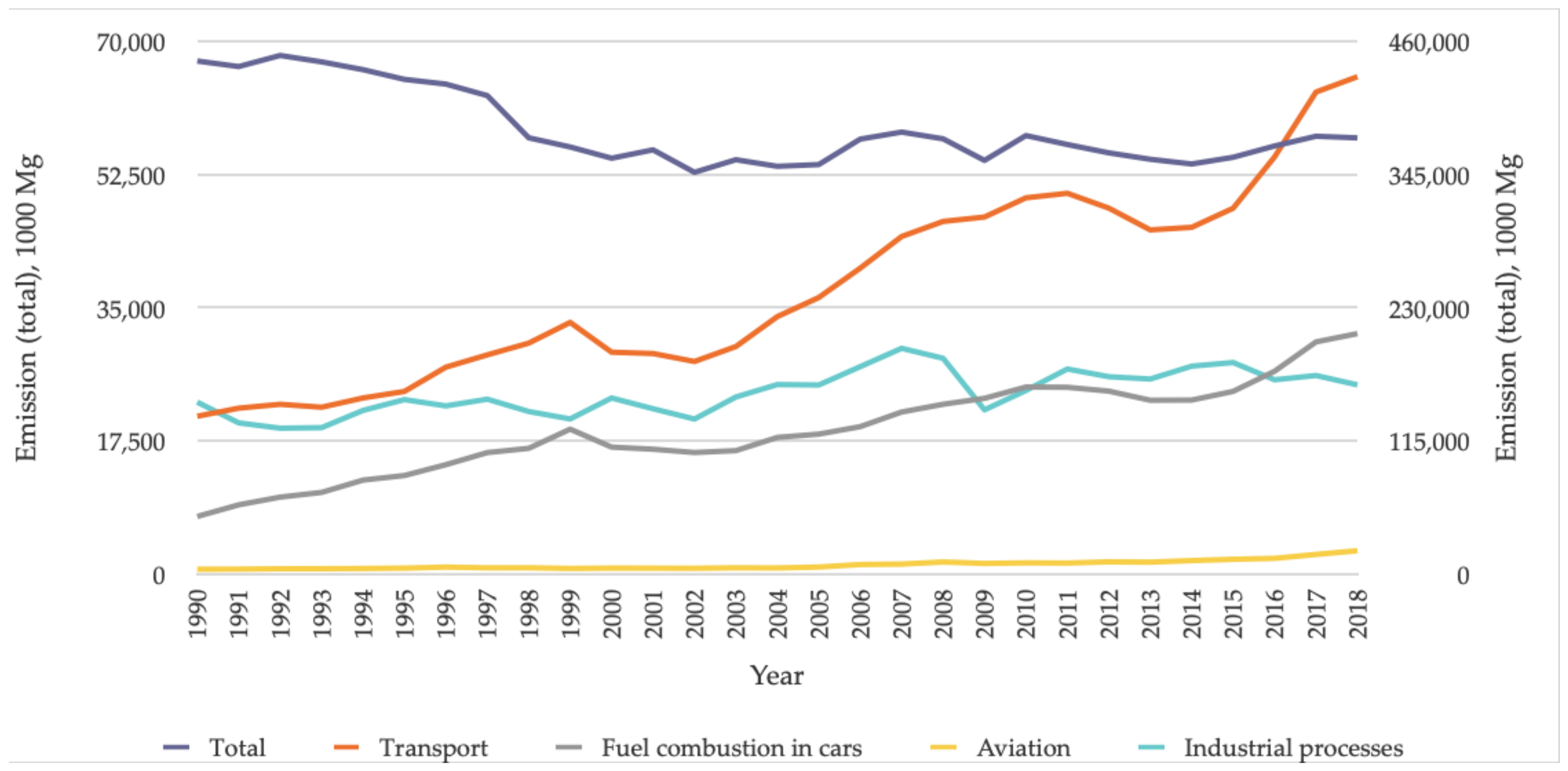
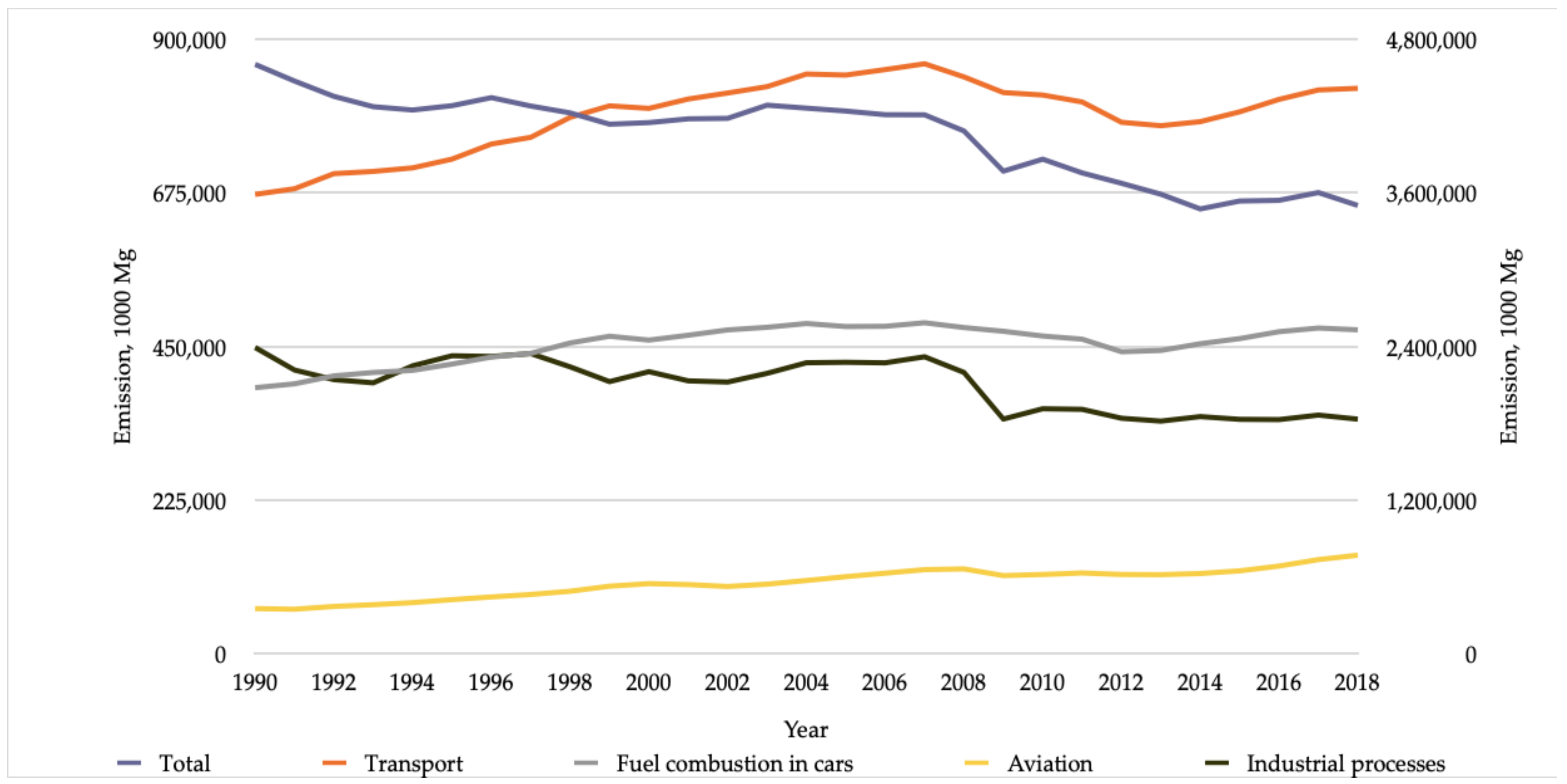
Since 1990, both in Poland and in other EU-27 countries, the total level of emissions has decreased by 15 and 24%, respectively. However, in the case of emissions from transport and industrial production, it systematically increased (Figure 1 and Figure 2), and in the years 1990–2018, it increased by the following:
- Fuel combustion in cars—314% (Poland), 22% (EU-27);
- Aviation—343% (Poland), 118% (EU-27);
- Industrial processes and product use—10% (Poland), decrease by 23–22% (EU-27);
- Transport—214% (Poland), 23% (EU-27).
Figure 1.
Gaseous air pollutant emissions in Poland. Based on data from Eurostat, European Environment Agency (EEA) [32].
Figure 1.
Gaseous air pollutant emissions in Poland. Based on data from Eurostat, European Environment Agency (EEA) [32].

Figure 2.
Gaseous air pollutant emissions in EU-27. Based on data from Eurostat, European Environment Agency (EEA) [32].
Figure 2.
Gaseous air pollutant emissions in EU-27. Based on data from Eurostat, European Environment Agency (EEA) [32].

The results of the analysis of the emission level during quarantine for each of the analyzed gases and PM2.5 particles are presented below.
3.1.1. Analysis of NO2 Emission Data
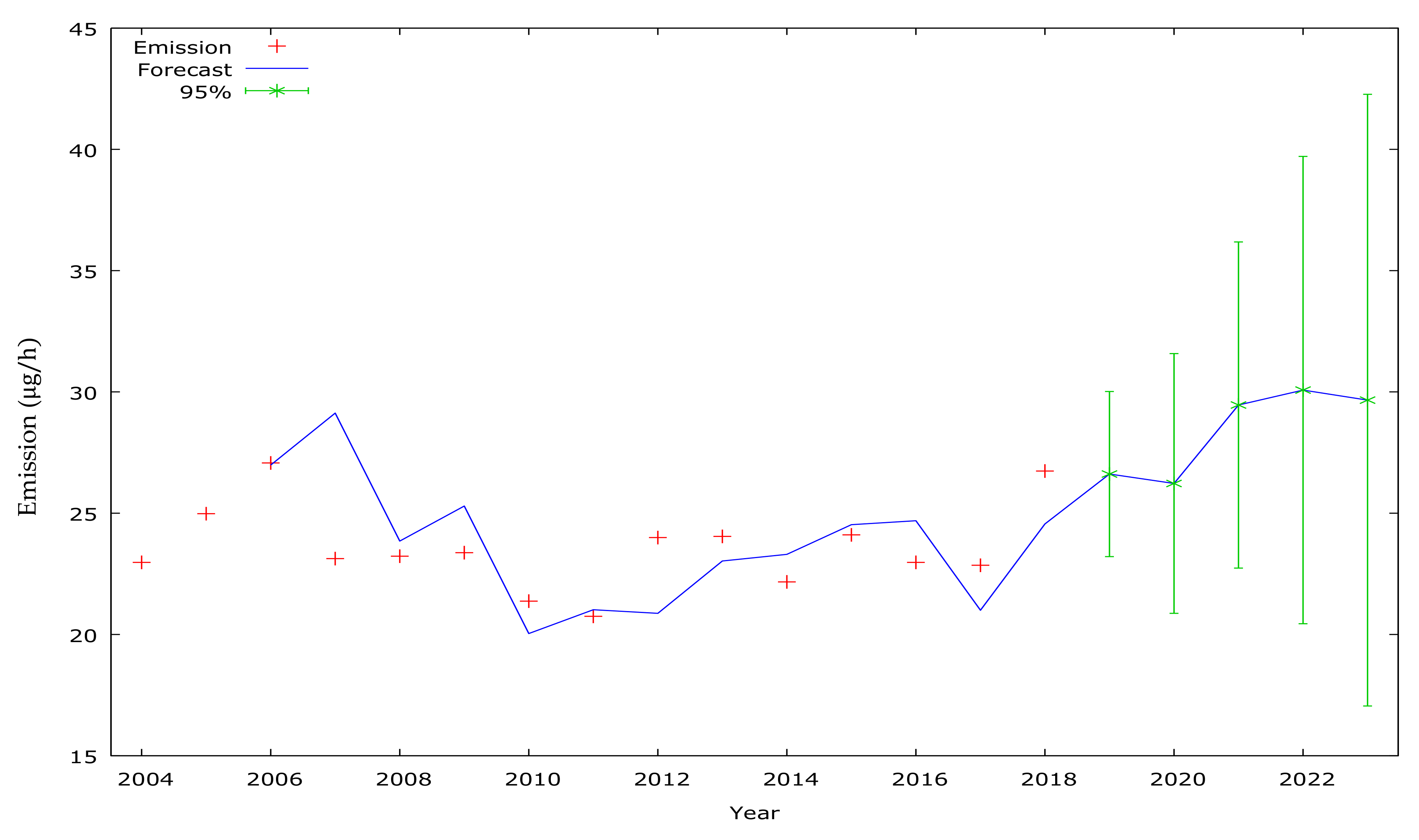
It is a gas harmful to the health and life of living organisms because it leads to hypoxia and generates allergic diseases. It leads to the formation of smog, which is a serious threat mainly in large cities [33,34]. The emission of nitrogen dioxide in Poland is generated mainly from the combustion of fossil fuels, both in industry and in transport [35]. In 2016–2018, nitrogen dioxide emissions in Poland increased by 16%. This was mainly due to the increase in the number of vehicles, many of which did not meet the European Union requirements due to their poor technical condition and age. Nitrogen oxides are also produced as a result of the use of nitrogen fertilizers in agriculture [36]. The emission limit is 200 µg/m3 with an averaging time of 1 h [37]. This level was to be achieved in 2010. Figure 3 presents two time series, i.e., empirical data on NO2 emissions in Poland in 2004–2018 and the forecast values obtained using the ARIMA model (2,2,0). Table 2 presents the parameters characterizing the models used in the article. The MAPE error indicates that the created models are reliable because it does not exceed 12% in each analyzed case. The Ljung–Box test confirms the lack of autocorrelation of residuals, while the Doornik–Hansen test confirms the normality of the residual distribution (where p is probability).
Indicators included in the table:
- Akeike information criterion, Hannan–Quinn information criterion, Schwarz information criterion: These information criteria are the most widely used. They are used to compare models of the dependent variable, in order to select the most accurate model. According to the adopted convention, the best model is the one for which the value of the information criterion is the lowest;
- MAPE—mean absolute percentage error;
- RMSE—root-mean-square error;
- Ljung–Box—statistical test of autocorrelations of a time series;
- Doornik–Hansen—test for normality.
The model used to forecast NO2 emissions until 2023 is characterized by an ex-post prediction error of 7%. The model can therefore be considered accurate. It is a model that will prove successful if the factors influencing the forecasted phenomenon remain unchanged (Figure 3).
It should be noted that according to the obtained forecast, NO2 emissions will increase in the coming years. In 2023, compared to the last known observation (2018), this increase was about 11%. At the same time, the chart presents the confidence interval. It is the range within which the predicted value can move with a 95 percent probability. The designated scope may constitute the information used to create scenarios for the development of the phenomenon.
3.1.2. Analysis of CO Emissions Data
Carbon monoxide is one of the main components of low emissions alongside carbon dioxide, heavy metals, t, nitrogen oxides, sulfur, and dioxins. Low emissions arise for two reasons: heat production, and the transport of goods and people [38,39]. Carbon monoxide, which is formed during the combustion of fuel in internal combustion engines, is the gas produced during combustion in an oxygen-poor atmosphere. It is a flammable gas and has no odor. As its emission occurs at heights below 40 m, high concentrations of pollutants exceeding safety standards may arise. Carbon monoxide is harmful to the health and life of living organisms and the environment. The emission limit for CO is 10,000 µg/m3. The volume of CO emissions in Poland has been subject to an upward trend in recent years.
It should be noted that the comparison of CO emissions in Poland and the EU-28 in 2015–2017 shows that in the case of the EU-28 averages, the emissions have remained stable over the past few years [32]. The same is true for other countries considered during the analysis, such as Germany, Italy, Spain, and France. In the case of Poland, CO emissions increased by approximately 5%.
The time series of CO emissions in Poland in the years 2004–2018 followed an upward trend (Figure 4). To forecast the amount of emissions in the coming years, the ARIMA model (2,2,0) was built. The model’s MAPE error is less than 12%. The obtained forecast in the most probable scenario (blue series of data) indicates an increase in carbon monoxide emissions in the forecast period. Therefore, it should be concluded that during the quarantine related to the COVID-19 pandemic, the emission level was consistent with the optimistic scenario defined by the 95% confidence interval of the forecast.
3.1.3. Analysis of Data on PM2.5 Particles Emissions
Particulate matter consists of fine particles suspended in the air (particulate matter—PM). PM10 particles consists of particles less than 10 microns in diameter, while PM2.5 consists of particles less than 2.5 microns in diameter. A total of 36 out of the 50 cities in the European Union with the highest PM2.5 concentrations are located in Poland. The authors analyzed the emission of PM2.5 due to its extremely negative impact on the health of living organisms. This particle reaches not only the upper and lower respiratory tract but also enters the bloodstream. It also often contains harmful substances, such as dioxins or heavy metals [40,41,42,43,44,45]. The permissible concentration of PM2.5 is 25 µg/m3, and this level was to be achieved in 2015. However, by 1 January 2020, it should be reduced to the level of 20 µg/m3.
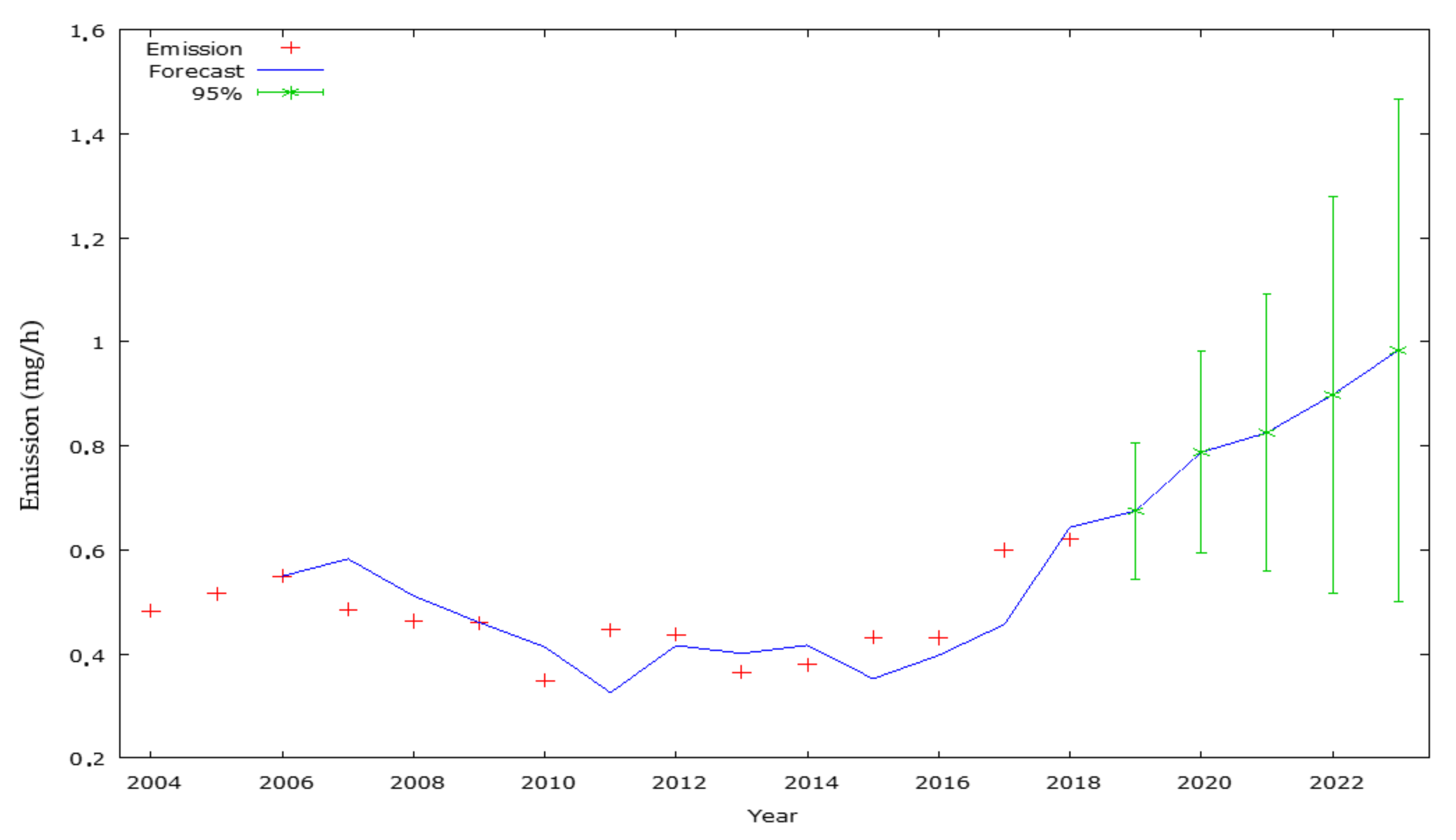
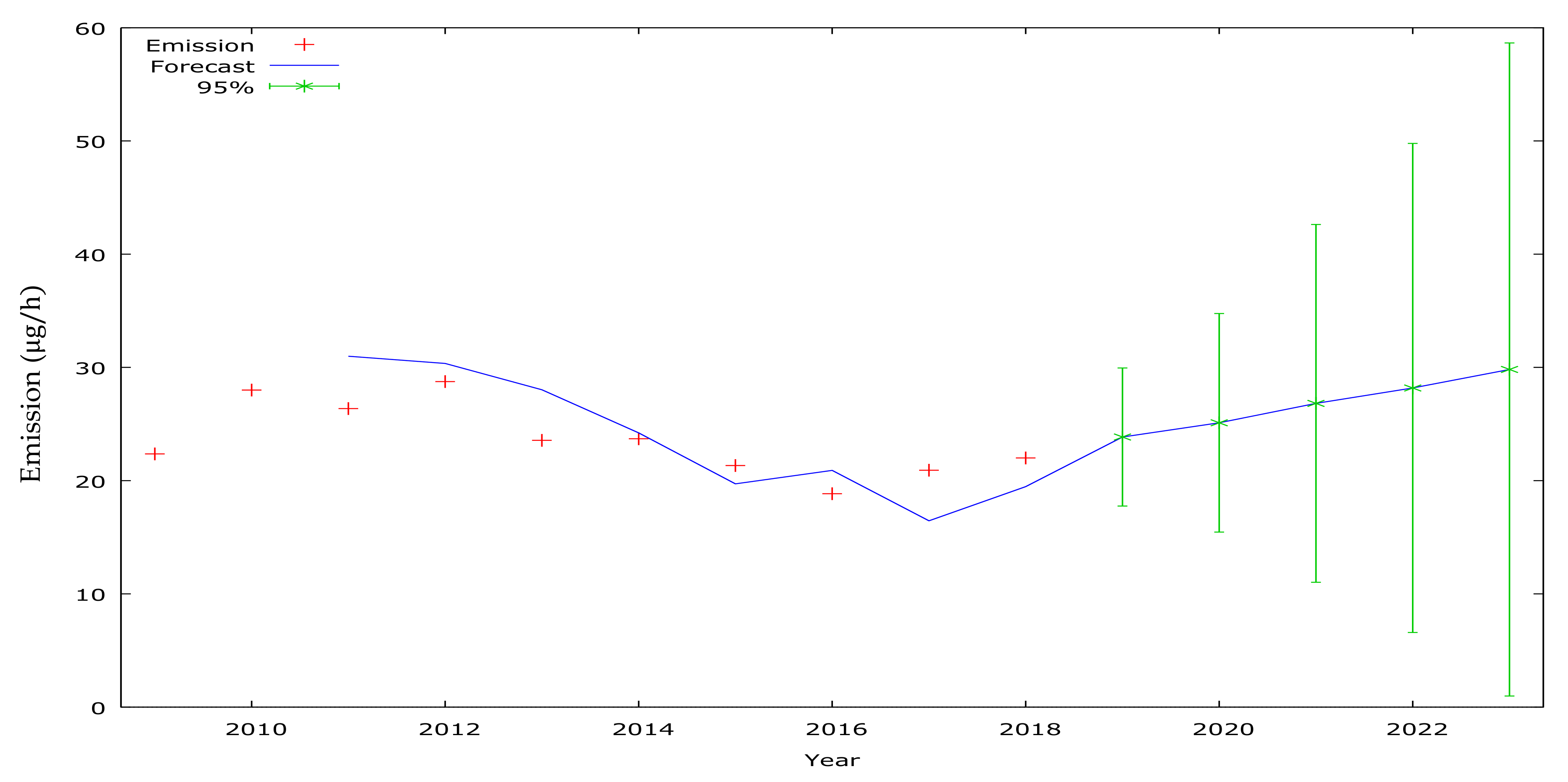
A mathematical model was created for the PM2.5 emission time series in 2009–2018 and a forecast for this series until 2023 (Figure 5). From 2016, the time series showed an upward trend. In 2016–2018, the emission increased by 15%. To create a forecast, the ARIMA model (1,2,0) was used. No change in the time series factors would lead to a further increase in emissions by less than 30% in 2023 compared to the last known observation.
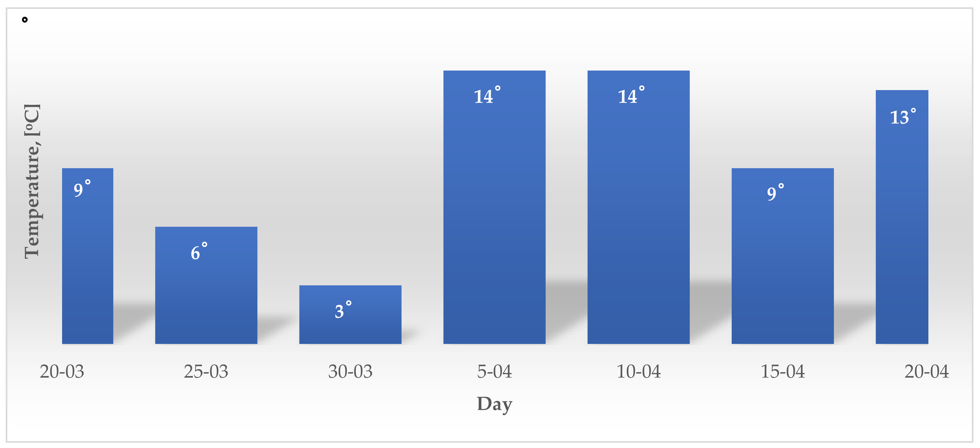
The emission of PM2.5 particles depends on the ambient temperature because its emission is mainly related to the activities of industrial power, as well as household furnaces. In the studied period in Poland, the temperature developments are presented in Figure 6.
It should be noted that the temperature forced the extension of the heating period at least until the end of April. This confirms the theory of a decrease in PM2.5 (and not only) emissions, mainly because of the reduced mobility of the Polish population.
3.1.4. Analysis of SO2 Emission Data
SO2 in Poland is generated mainly during combustion processes in coal-fired power plants. It should be noted that the emission of oxides of this type decreases every year. In the years 2008–2018, this decline in Warsaw was over 50%. It is also a typical trend for the European Union average. Despite this, the level of sulfur dioxide in Poland is higher than in other EU countries. The permissible level of SO2 emission is 350 µg/m3 with an averaging time of 1 h.
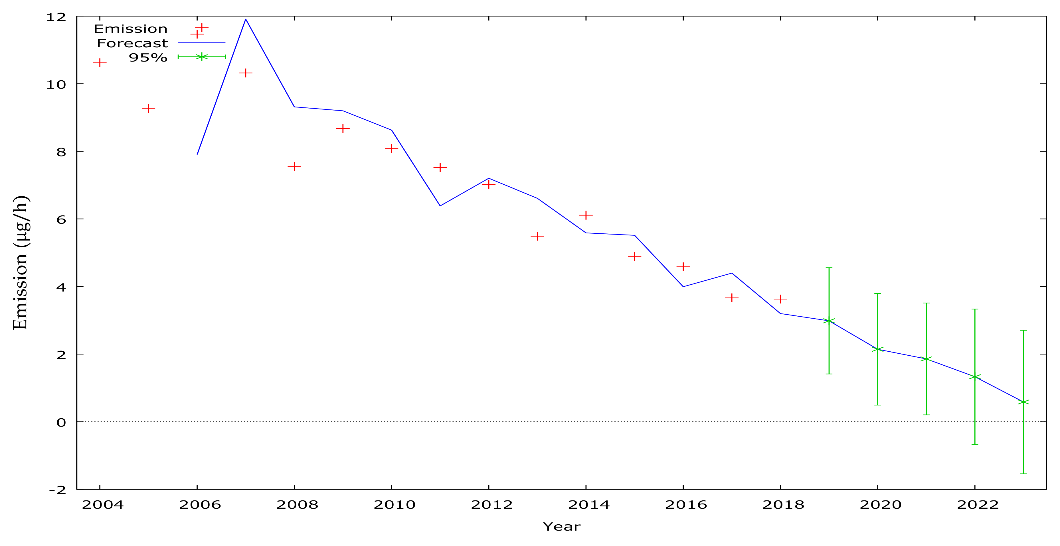
Furthermore, in the case of SO2, a mathematical model of the emission time series in 2004–2018 was built, and on its basis, the forecast of this series until 2023 (Figure 7). The ARIMA model (2,2,1) was used. Among the models presented in the article, it is characterized by the highest error rate, i.e., over 14%. The forecast indicates that until 2022, a continuation of the downward trend in the time series of sulfur dioxide emissions in Poland can be expected. Compared to the last known observation, i.e., 2018, the presented forecast indicates an 86% decrease in emissions in 2023 if the trend is not disturbed.
3.2. Spatial Analysis of Air Pollution
Using statistical data on the state of the atmosphere obtained from the Copernicus Atmosphere Monitoring Service (CAMS), thermal maps of the pollution level for the studied time periods were created by the authors [47]. The WGS 84, EPSG 4326 coordinate system and linear interpolation were used to generate the thermal maps. The display mode has been set to a single channel pseudocolor. The data include the following parameters: CAMS daily air quality analyses, median ensemble model, gridded data type, and surface level time 6 h.
3.2.1. NO2
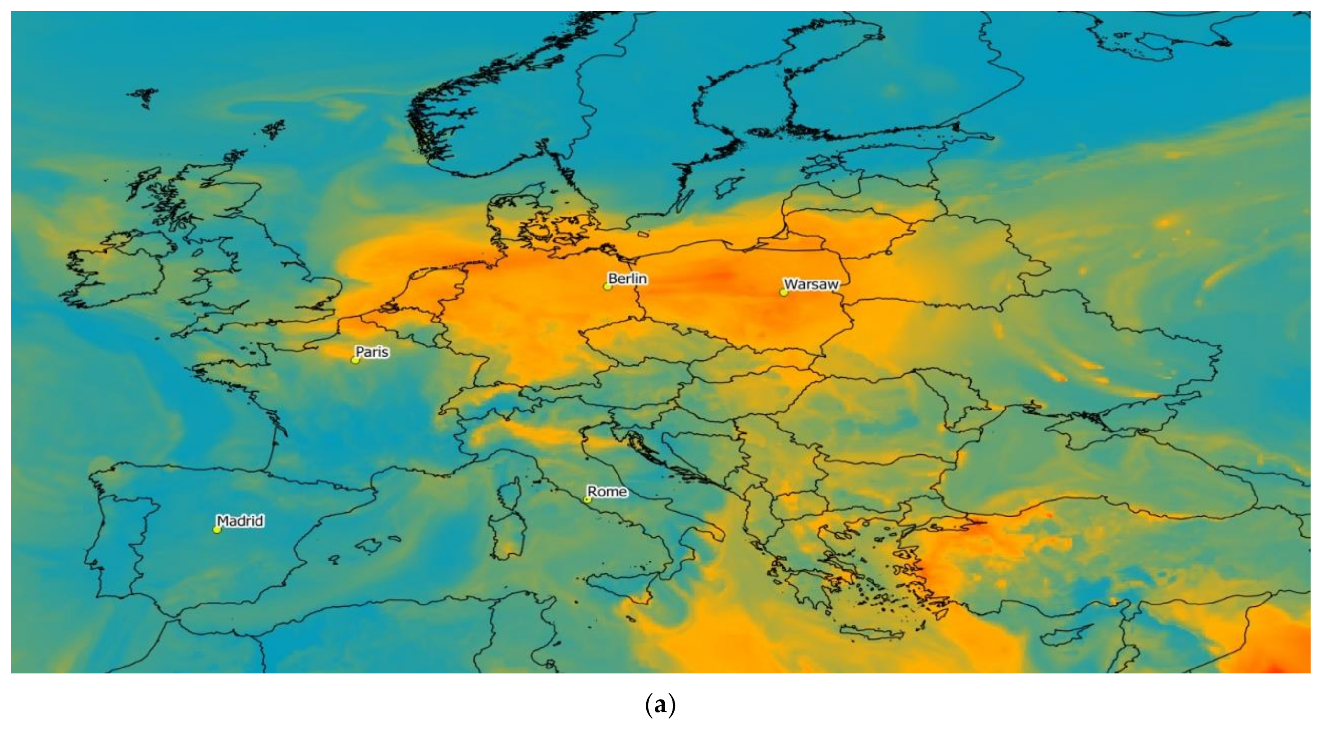
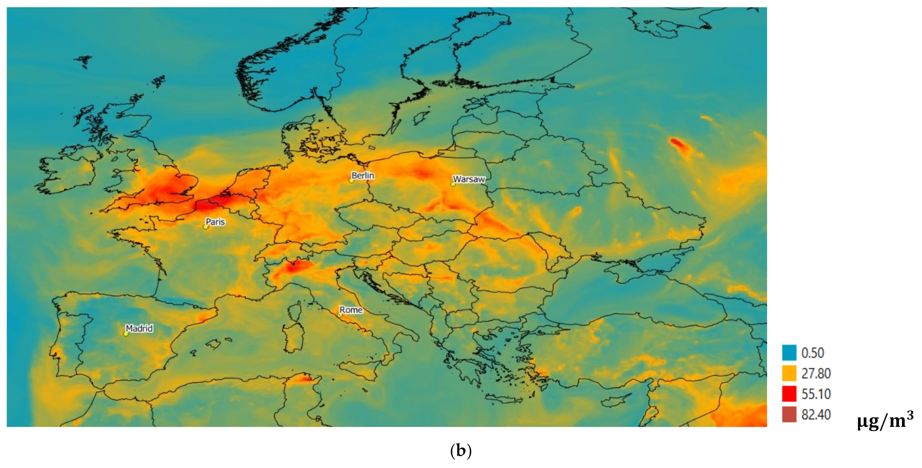
An exemplary map for NO2 is shown in Figure 8. The maps show the following layers:
- Raster layer with NO2 concentration data;
- Polygonal vector layer containing the borders of individual countries;
- Point vector layer with marked capitals of selected EU countries.
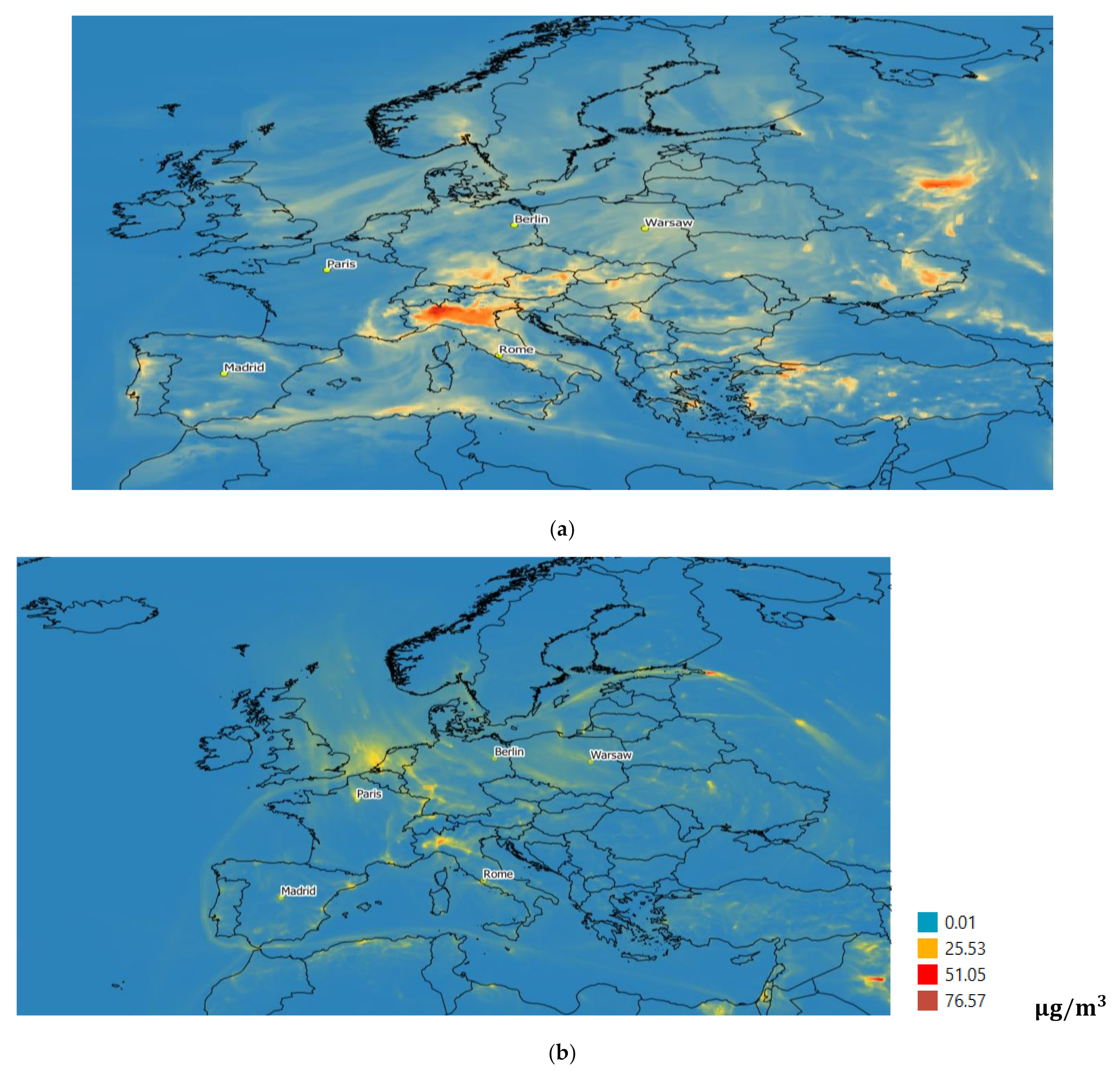
Comparing the created heat maps from 5 April 2018, and 2020, it can be stated that the NO2 concentration has significantly decreased in Poland, Germany, and France. By contrast, in Italy and Spain, it has increased.
Table 3 presents a comparison of the level of concentration of this gas in 2018 and 2020 in selected capital cities of the European Union. It should be noted that we are dealing with a change in the upward trend in Warsaw, Berlin, and Paris. However, in Rome and Madrid, the upward trend continued.
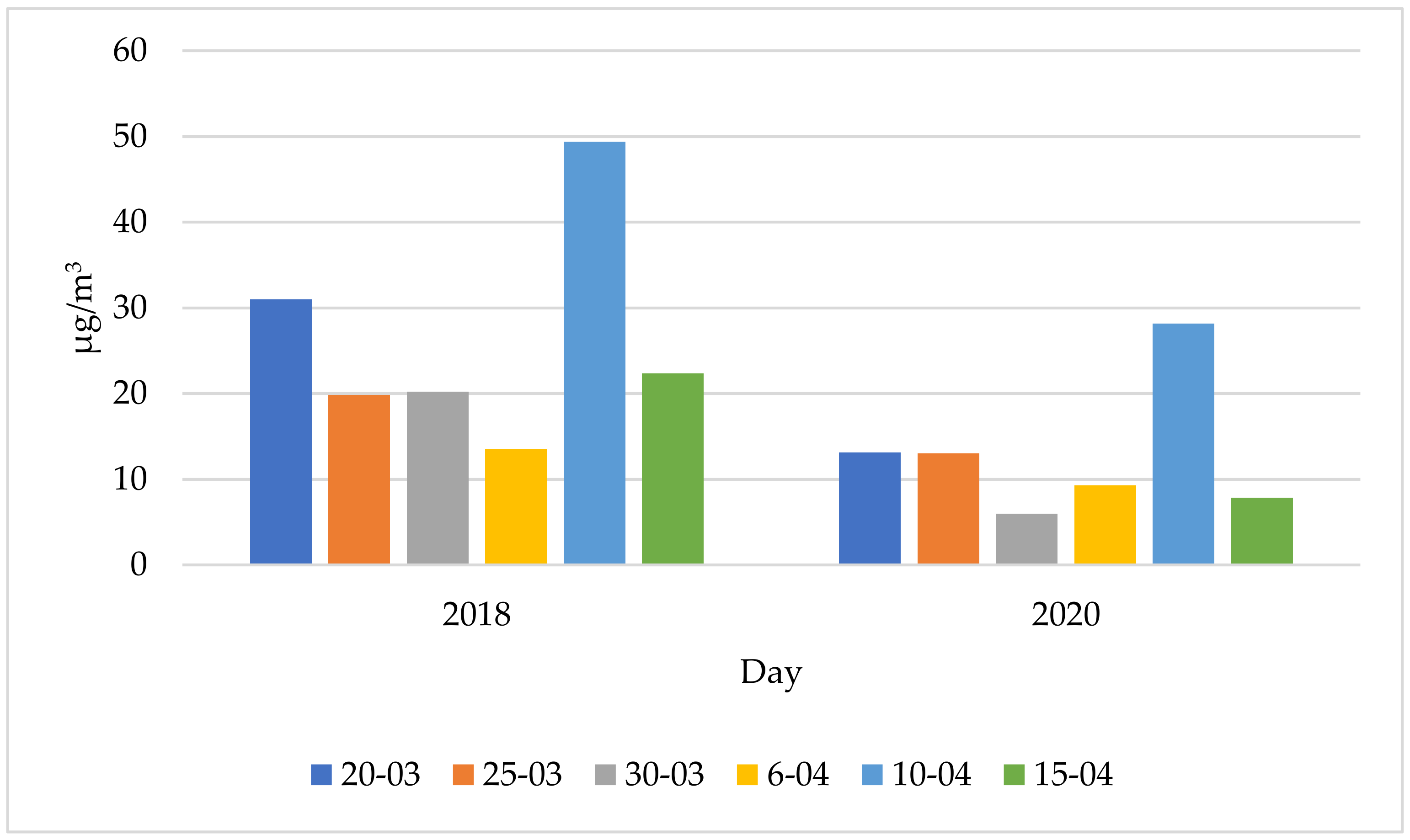
Additionally, Figure 9 presents a comparison of the NO2 concentration in Warsaw. It was stated that the concentration decrease was the largest (among the analyzed cities) during March and April 2020 compared to the base year, which was assumed to be 2018. It should be noted that on each of the analyzed days the concentration was halved in 2020. The biggest drop was recorded on 30 March, when the concentration fell by 70%.
3.2.2. CO
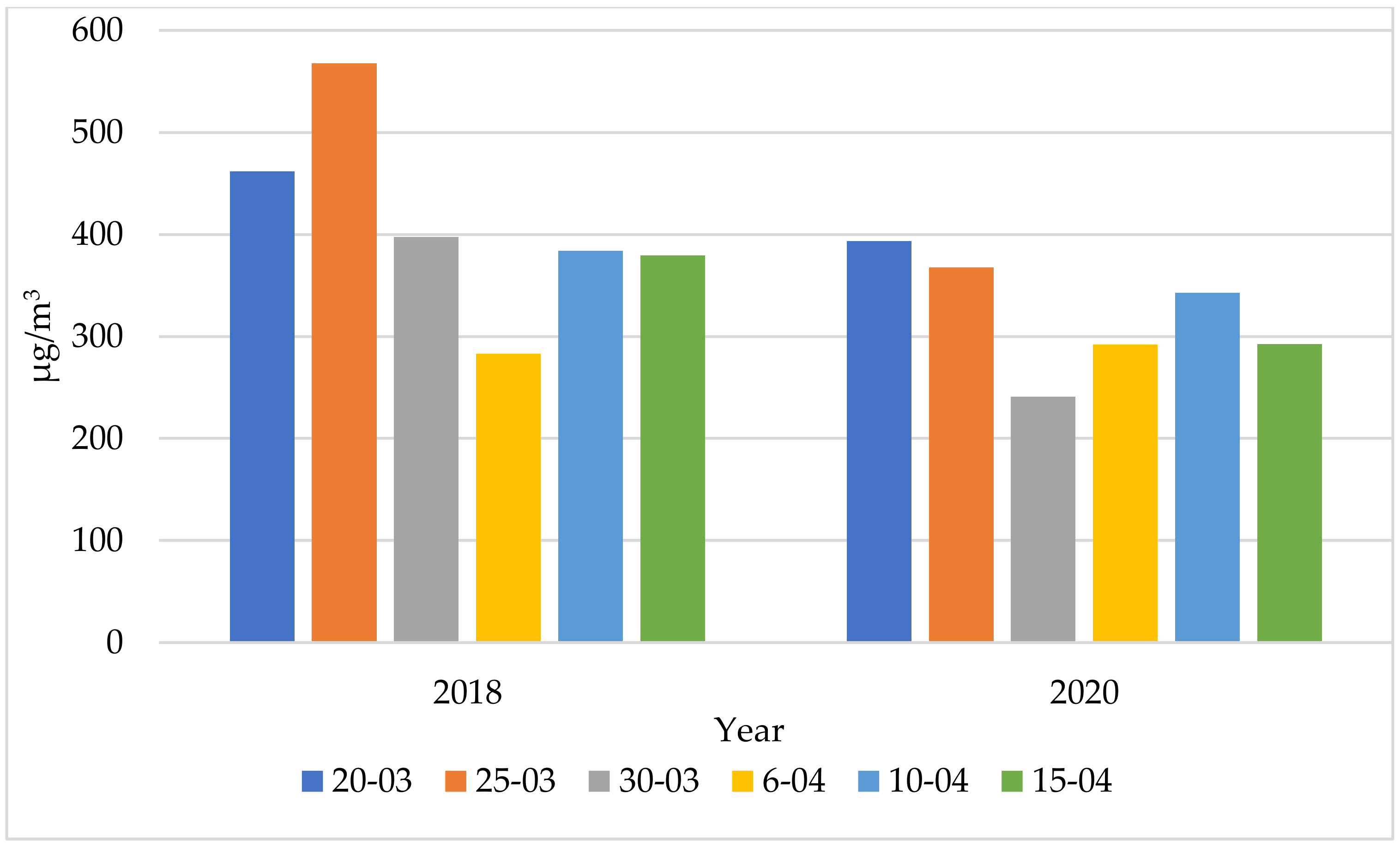
Table 4 presents a comparison of the concentration level in the time selected for the analysis (from 20 March to 15 April). As a result of the quarantine, the carbon monoxide concentration decreased in Berlin (the decrease was the greatest), Warsaw, and Paris. Again, a rising concentration can be seen in Rome and Madrid.
The heat maps also make it possible to observe with the naked eye the difference in the level of concentration in the studied years. Remembering the maps from 2018 and 2020, a significant decrease in the CO concentration can be found in Germany, Poland, and France. However, in other countries, especially in Italy, an increase in CO concentration was observed.
Figure 10 shows the thermal map of CO concentration for 5 April 2018, and 2020.
The concentration level in the analyzed period in Poland decreased, which is shown in Figure 11. The largest decrease was recorded on 30 March 2020, when the concentration decreased by about 40%, compared to 2018. The average decrease on 20 March to 15 April was 12%.
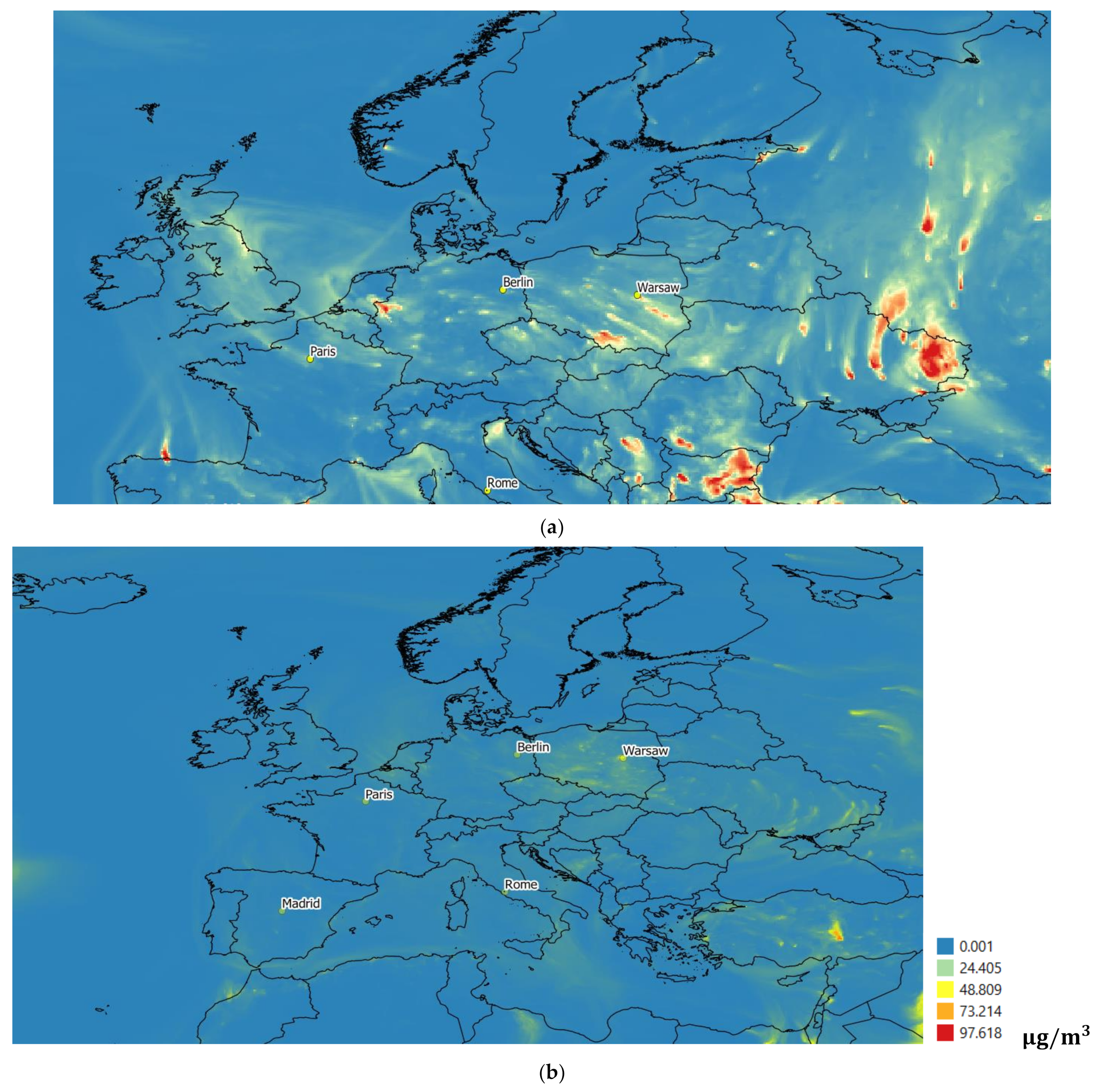
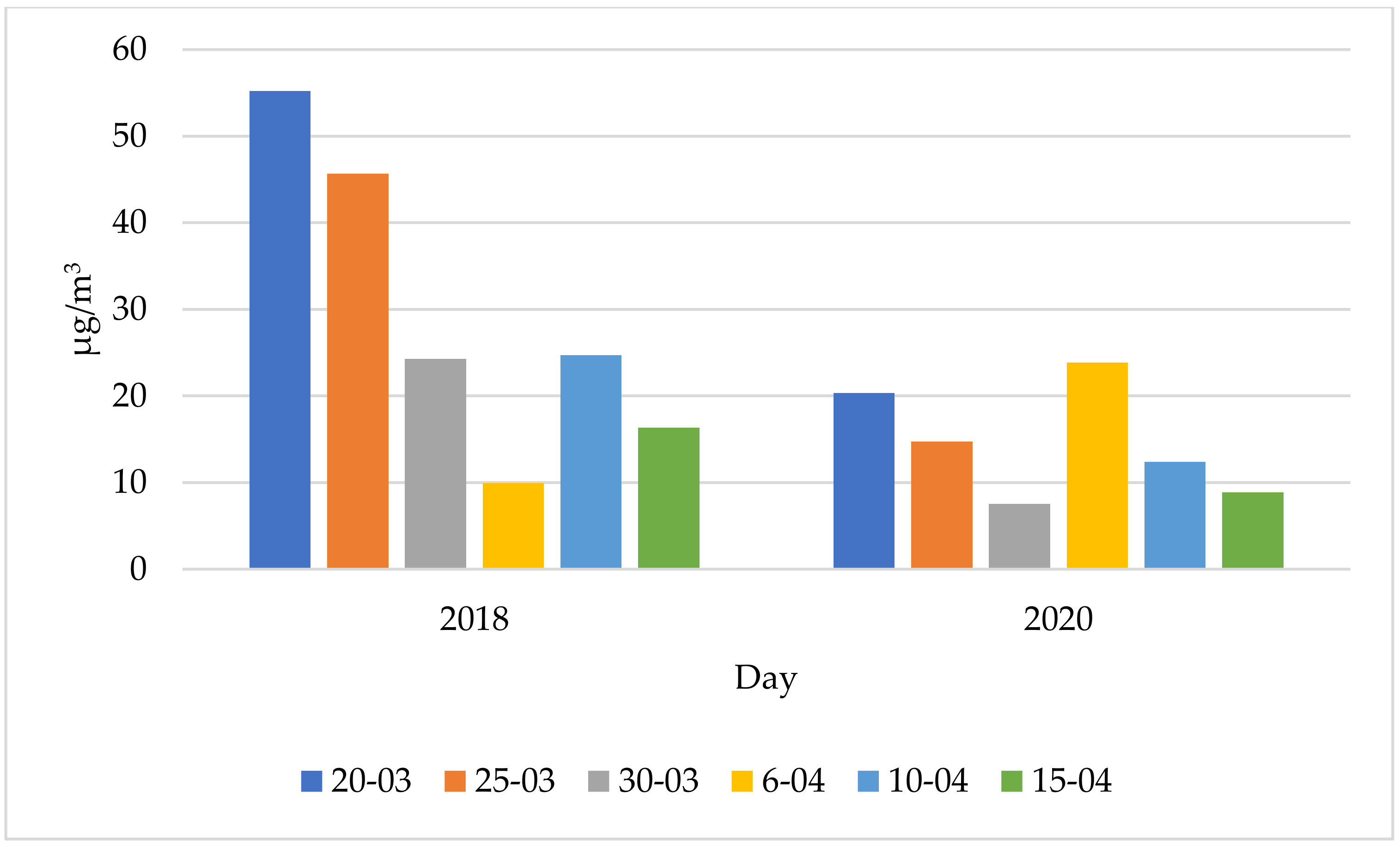
3.2.3. PM2.5
It should be noted that the EU average of PM2.5 concentration in 2015–2017, expressed in grams per one euro, is almost five times lower than the average concentration in Poland. In turn, Table 5 contains information on the concentration level PM2.5 in the period from 20 March to 15 April in 2018 and 2020. Again, the concentration decreased in Berlin, Paris, and Warsaw, with the decrease being the most favorable for Warsaw. The increase in PM2.5 concentration was recorded in Rome and Madrid, where it increased by over 100%.
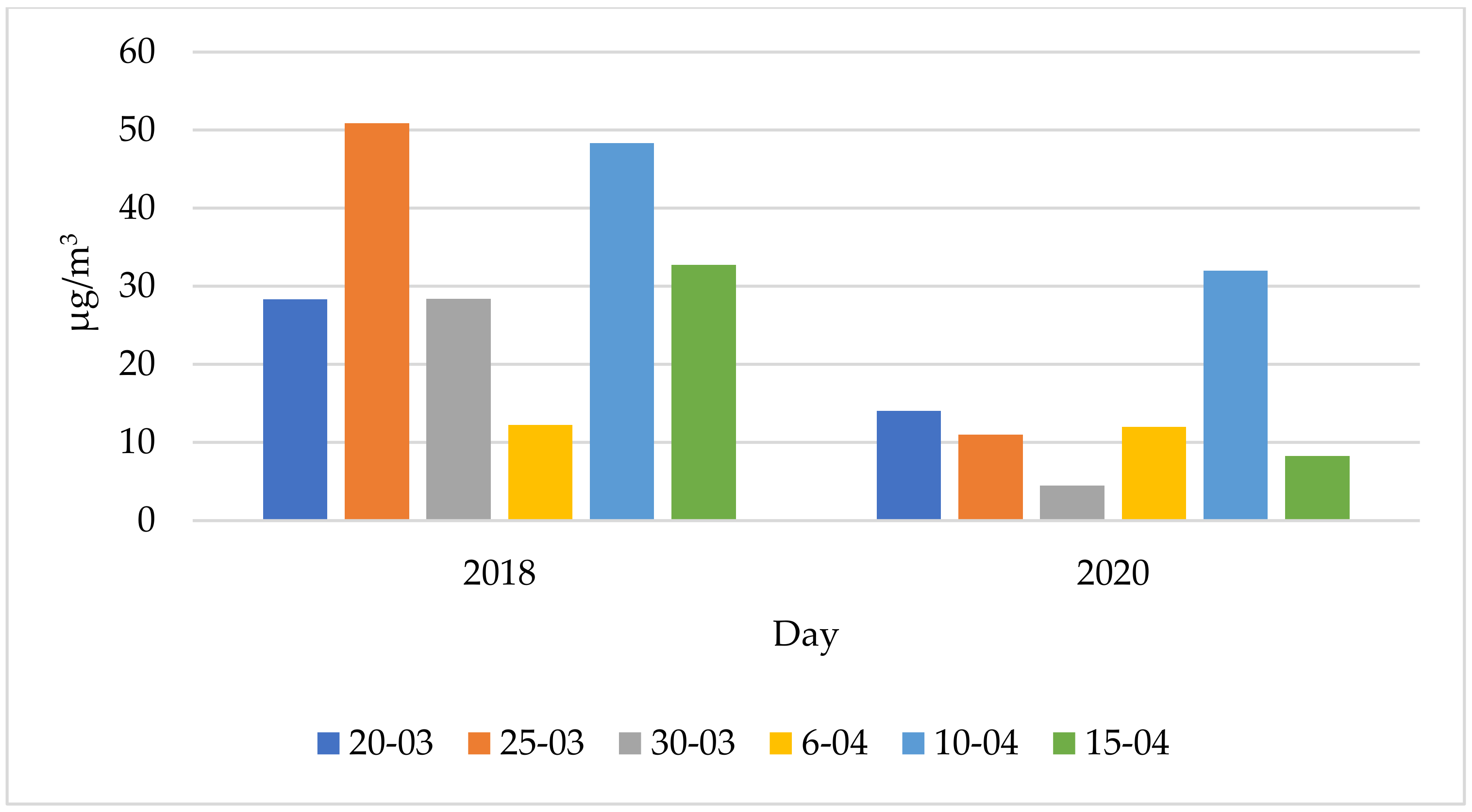
In the case of Warsaw, the decrease in each of the analyzed days was very significant (minimum 33%), the maximum decrease was 84% and occurred again on 30 March 2020, as in the case of the previously analyzed gases (Figure 12).
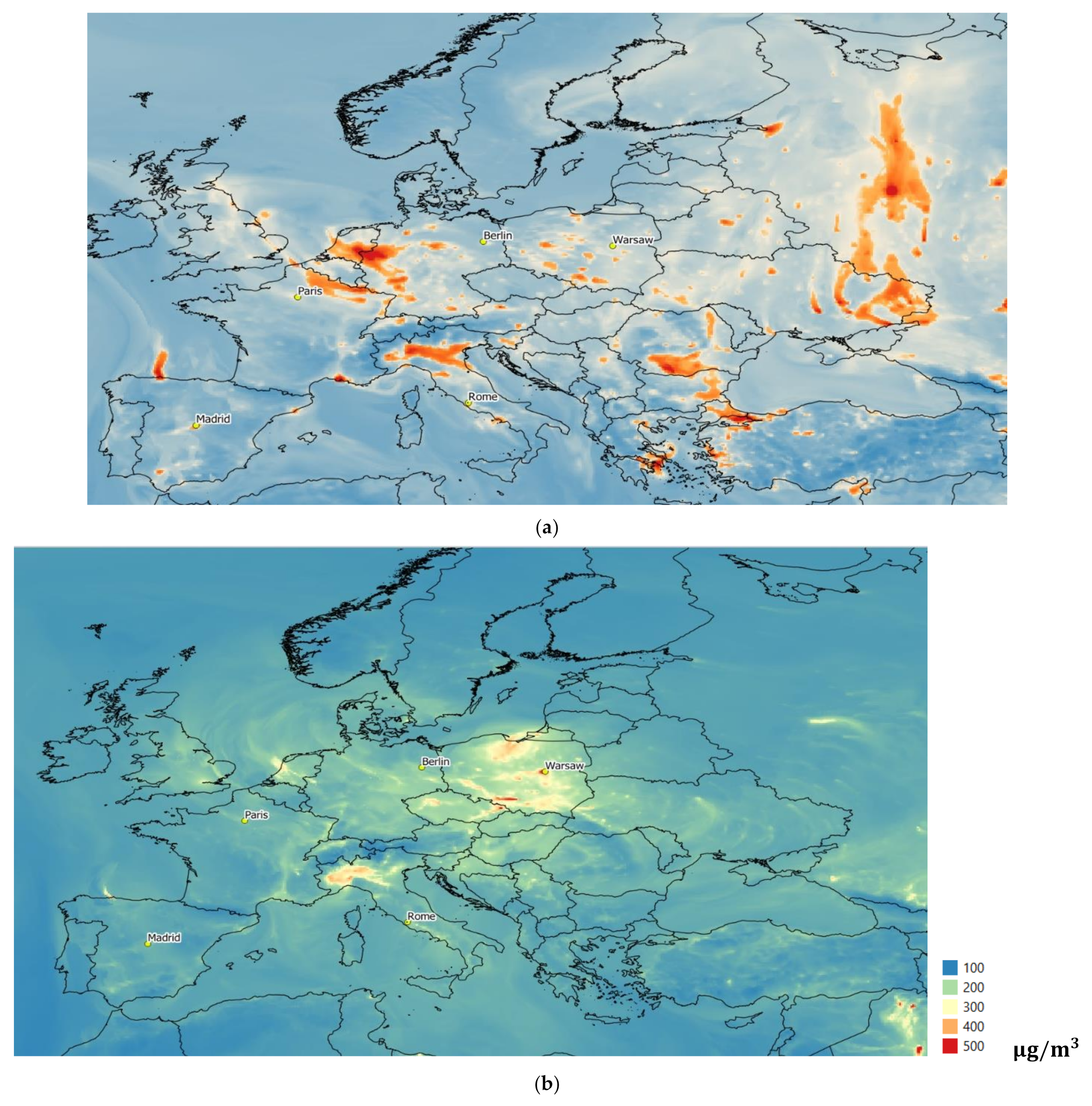
Figure 13 shows the heat map for 10 April in 2018 and 2020. Moreover, in this case, the trends presented in Table 4 can be seen, i.e., significant decreases in PM2.5 concentrations were recorded in Poland and Germany, a slight decrease in France, while in Italy, and in particular in Spain, significant increases were noted.
3.2.4. SO2
Table 6 presents a comparison of SO2 concentrations in selected capitals of the EU Member Countries on 20 March to 15 April 2018, and 2020. In this case, all analyzed places showed a downward trend in concentration. However, it should be considered that SO2 concentrations are falling in the EU, irrespective of the coronavirus pandemic.
Figure 14 shows the thermal maps of SO2 concentration in Poland on 5 April 2018 and the same day in 2020. Again, the visual analysis shows a decrease in the intensity of the analyzed phenomenon, i.e., the sulfur dioxide concentration, especially in Poland, Spain, and Germany, and then Italy and France.
Figure 15 shows a comparison of SO2 concentration in Warsaw on selected days from 20 March to 15 April in 2018 and 2020. It was found that the sulfur dioxide concentration in Warsaw on the days selected for the analysis dropped by as much as 70%, except on 6 April 2020, when it was more than twice as high as in the base year, 2018.
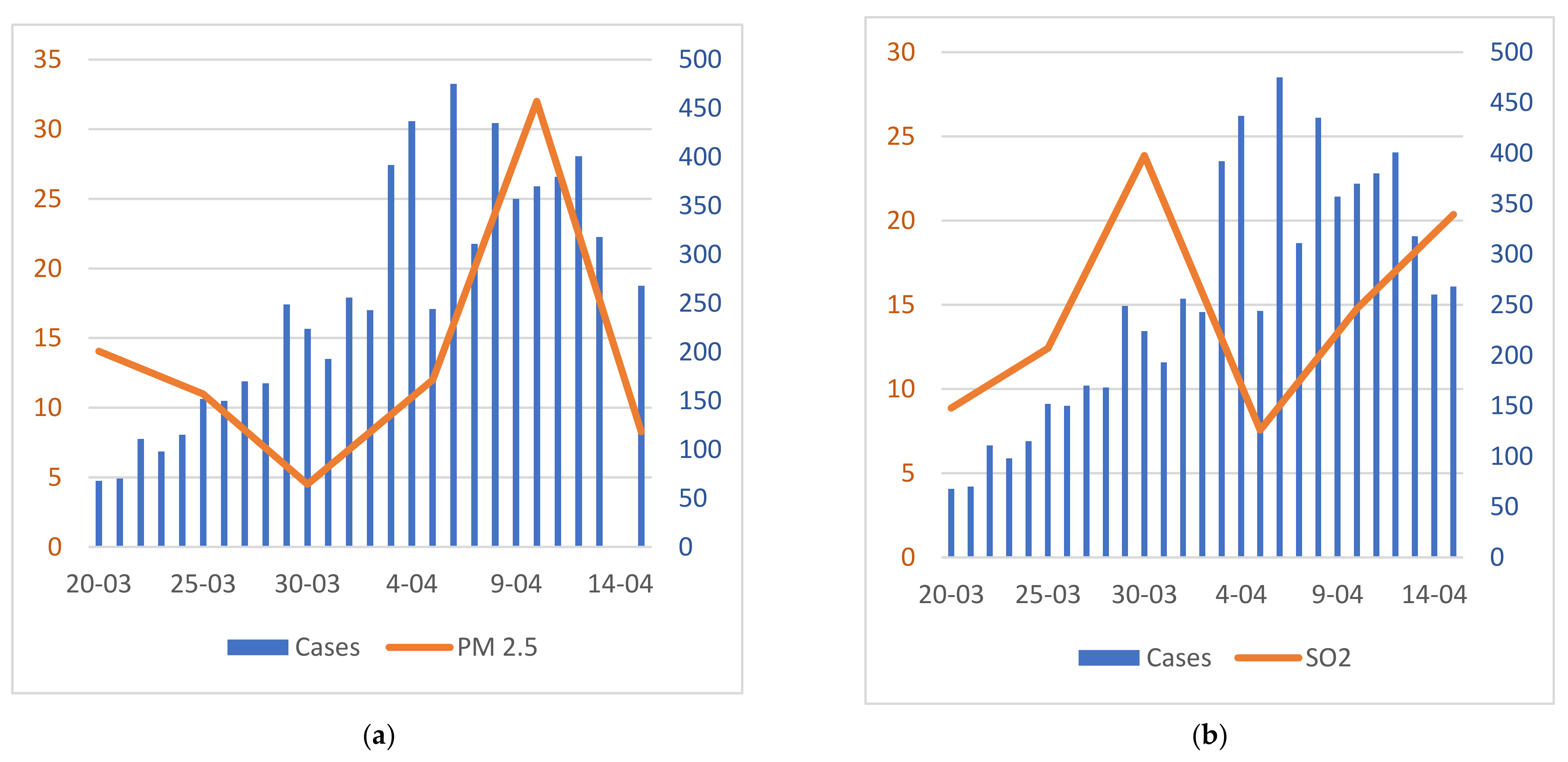
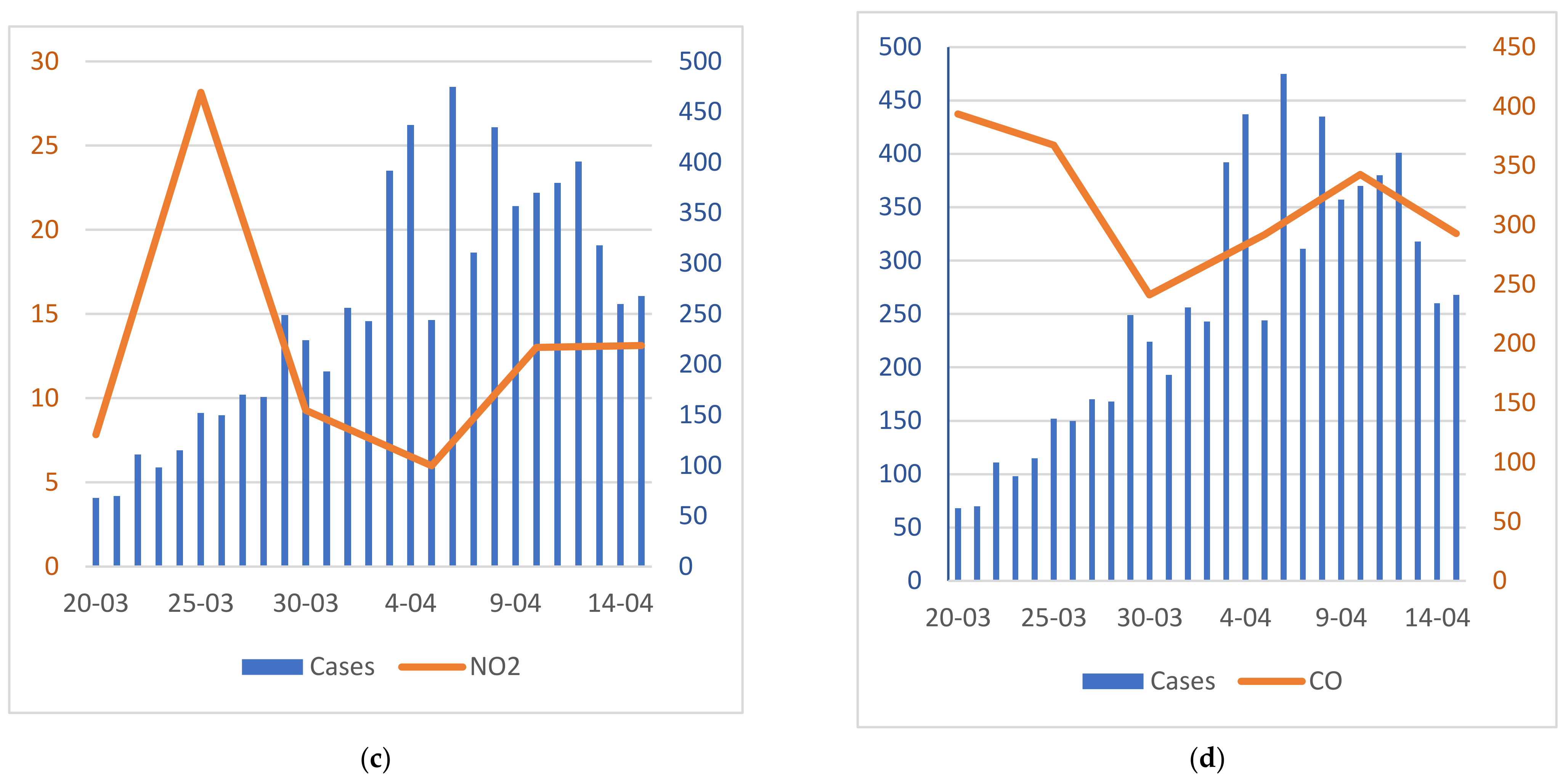
To summarize the above analysis, a comparison of the number of COVID-19 cases in Poland and the concentration of the analyzed substances was made (Figure 16).
There is a clear correlation between the values presented in Figure 16, especially in the case of nitrogen dioxide, but also sulfur dioxide. It can therefore be seen in the case of SO2 that, despite the general downward trend in this time series, the concentrations decreased during the quarantine period. Around 10 April, the concentrations increased for all substances. That day was Good Friday (the beginning of Easter), and in Poland, there was no ban on moving away from home.
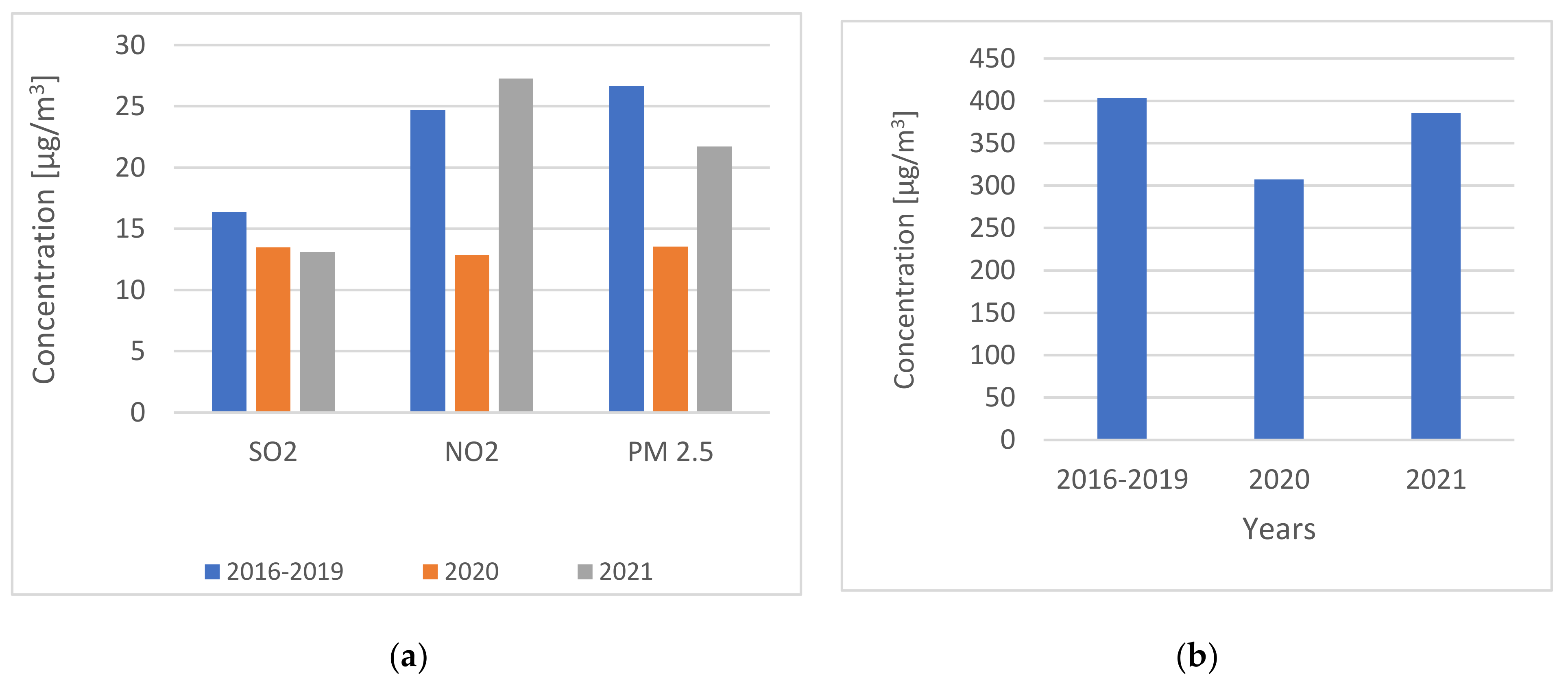
Additionally, for Poland, a comparison of the tested substances concentration level with the average concentration in years 2016–2019 and the lockdown period in 2021 was made (Figure 17). It should be noted that for NO2 and PM2.5, there was an almost 50% decrease in concentration in 2020, compared to the previous years. In 2020, the concentration of CO decreased also by approximately 25%. The downward trend for SO2 was maintained.
The re-tightening of safety rules in Poland took place on 25 March 2021. The reason for this decision was Easter and a significant daily increase in COVID-19 cases, with the simultaneous lower hospital bed and respirator capacity. However, compared to the same period of the previous year, the restrictions were much less restrictive. They also concerned individual voivodeships. The analysis of the concentration level in 2021 shows that the epidemic has become part of everyday life and citizens have ceased to comply with the imposed restrictions. There has been no decrease in the mobility of the society; on the contrary, the increase in NO2 and PM2.5 emissions confirms the return to the growing trend from previous years (Figure 17).
3.3. Scenarios for the Emission of Selected Gases and PM2.5 Particles
The forecasts and designated confidence intervals presented in Section 3.1 were used to create the scenarios for the emission of selected gases and PM2.5 particles. The scenarios are a combination of the created forecasts (the most probable scenario) and the constructed confidence intervals (optimistic and pessimistic scenarios). Additionally, the authors simulated the impact of quarantine on the levels of gas and PM2.5 emissions. The highest determined percentage decrease was used as input data for the simulation for the COVID-19 effect scenario o, while the lowest emission decrease was used for the pessimistic COVID-19 effect scenario p.
The assumptions that were made when creating individual scenarios are presented in Section 2.3.
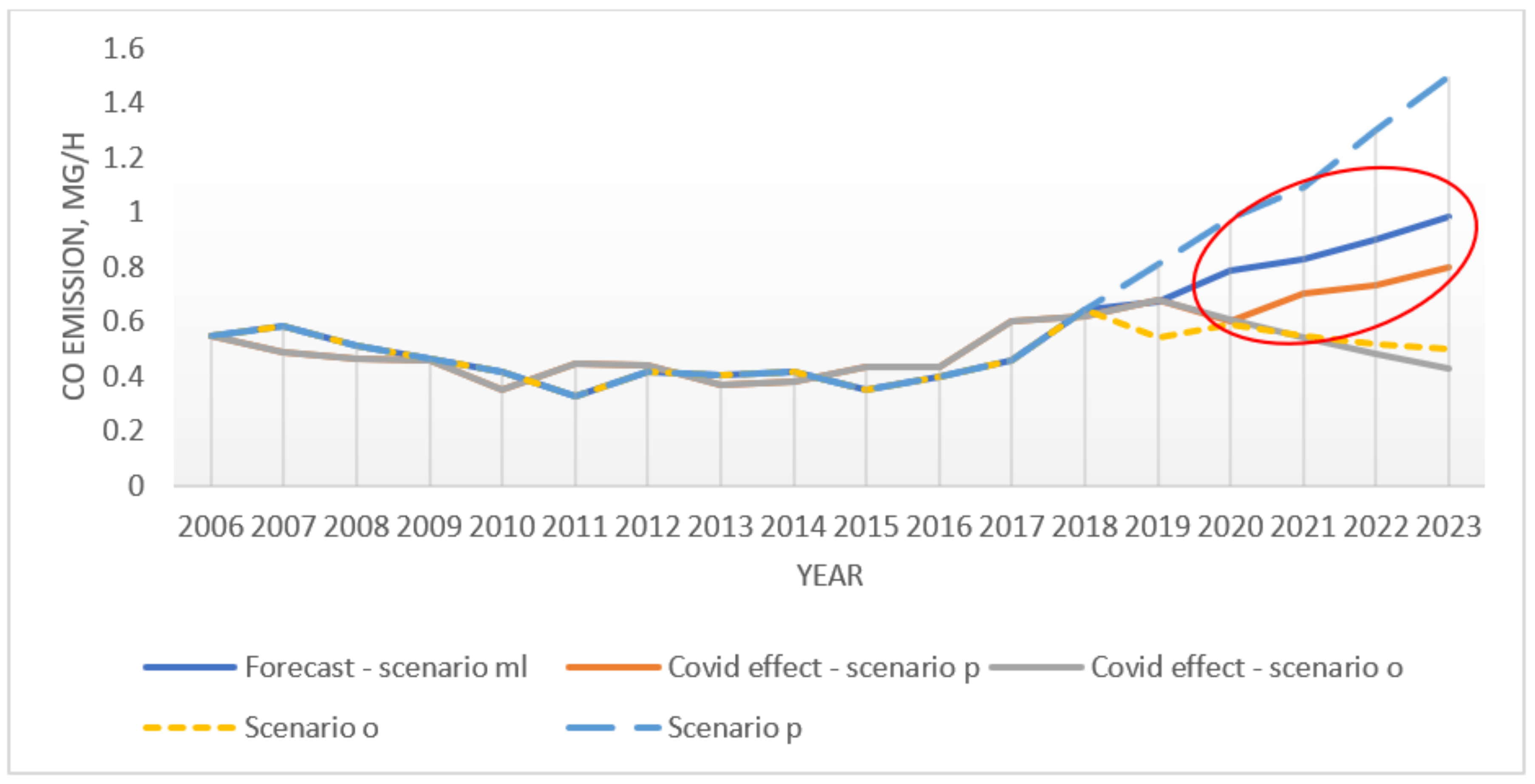
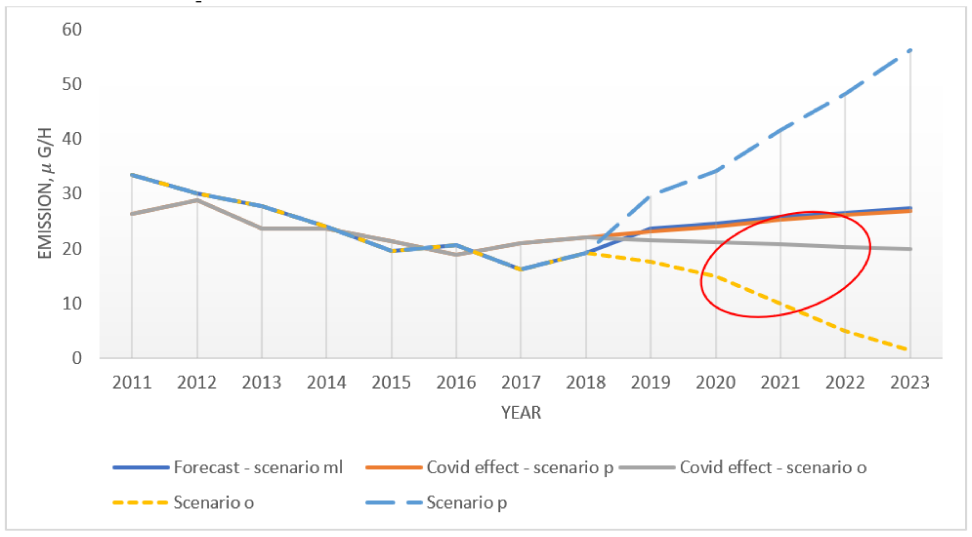
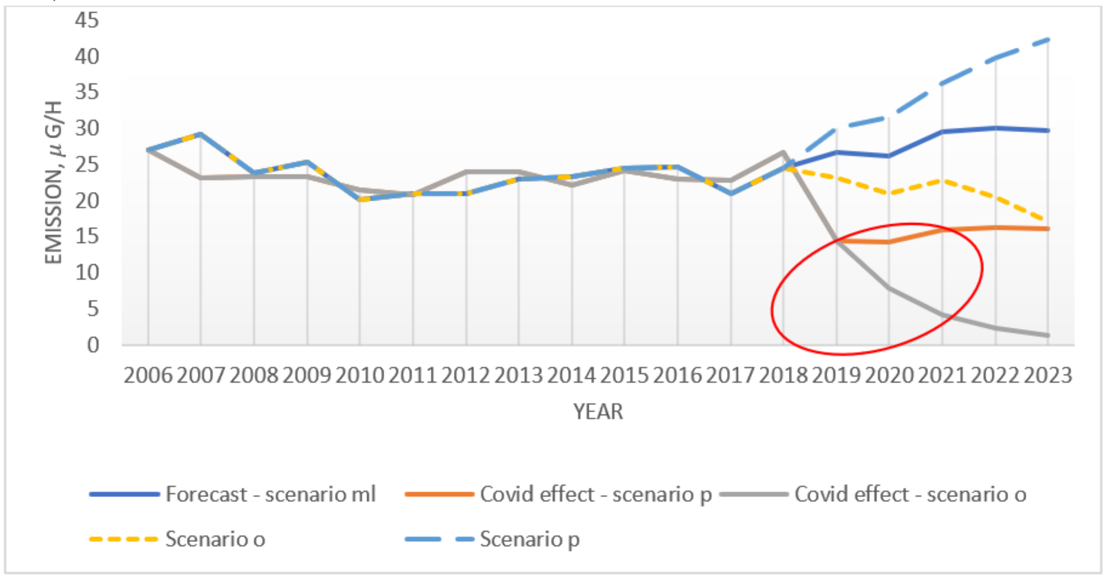
The results of the simulation are presented in Figure 18, Figure 19 and Figure 20. The effect of changes related to the pandemic is circled in red on the graphs to further facilitate their visual analysis. The level of the projected emission was reduced by the smallest decrease in this emission that was recorded on 20–25 March 2020, that is, for the following:
- CO by 11%: Therefore, if the insulation condition was maintained, the average emission in 2023 would be 0.79 instead of 0.98 mg/h. If we consider the optimistic scenario, it would be 0.41 mg/h.
- In the “optimistic scenario o” in 2023, the emission is 17% higher than in the “COVID-19 effect—scenario o”, while in the “p scenario” the emission is almost twice as high as in the “COVID-19 effect—scenario p”.
- PM2.5 by 2%: If the quarantine status was maintained in the pessimistic scenario, the average emission in 2023 would be 26.9 instead of 27.5 mg/h, while in the optimistic scenario, it would be 19.9 mg/h, which is a decrease of less than 28%.
- In the scenarios obtained based on the confidence interval, the greatest dispersion of values was obtained. In the optimistic scenario, in 2023, the emission is lower than the forecast by about 90%, and in the pessimistic scenario, twice as much.
- The effect of reducing NO2 emissions in the “COVID-19 effect” scenarios is much more significant than in “scenario o”. In this case, compared to the forecast value, the emission decreased by 57%, and in the pessimistic scenario, it increased by 42%.
4. Discussion
The article presents the effects of the unprecedented phenomenon of social isolation on a global scale. In Poland, the period of strict COVID-19 quarantine fell on 20–25 March 2020. The impact of this phenomenon on the level of gaseous and solid air pollutants in Poland and selected European Union countries was analyzed. The analyzed period was compared with the base year, which was assumed to be 2018. It was noticed that in Poland, the concentration of such gases as CO, NO2, and PM2.5 particles decreased. A similar trend was also revealed in the case of Germany and France. The isolation decreased the consumption of crude oil, natural gas, and other petroleum products. This was due to the limitation of the mobility of the inhabitants of the European Union, as well as limitations in electricity consumption. The coronavirus pandemic caused a decrease in the demand for hard coal in Poland. Tauron, one of the largest Polish electricity companies, was forced to reduce working time in both the mining and generation segments. It was a result of the decline in electricity demand all over the world [48]. The authors analyzed the temperature course during the research period. The analysis showed that the heating period was extended due to the relatively low air temperature. Therefore, the concentration caused by heating had no influence on the results of the concentration level. However, as already mentioned, in the analyzed period, a decrease in the demand for electricity was noticed. Activities related to anti-virus prevention directly contributed to the reduction in electricity consumption. Production in many industrial plants has been reduced, as well as the activities of service points, shops, shopping centers, airports, stations, schools, universities, etc.
The increase in gaseous and solid air pollutants concentrations from 20 March to 15 April was recorded in 2020 in relation to 2018 in Rome and Madrid. The reason for this situation was most likely noncompliance with the quarantine and restrictions aimed at reducing the number of cases of COVID-19. Spaniards and Italians broke the introduced bans en masse, as evidenced by the reports on the number of fines issued by the police during that period. This, of course, had negative repercussions of more infections and the spread of the epidemic. In contrast, SO2 concentration decreased in all considered countries. This phenomenon is related to the overall decrease in sulfur dioxide concentration, which has been going on for many years.
As in the case of CO, the increase in emissions is influenced by using obsolete furnaces. In addition, it is also caused by the increased transport of people and goods and the growing number of diesel vehicles, often old, produced more than 10 years ago [49]. Such cars, unlike new ones, have an extremely harmful effect on the environment [50,51]. A particularly high increase in second-hand car imports has been recorded since the abolition of the recycling levy. The year 2020 was a record year regarding the number of cars imported from abroad. Compared to January 2019, imports in 2020 were increased by approximately 9%. After that, the number of imported cars decreased because of the safety measures due to the pandemic. It was mainly caused by additional procedures at the borders: the necessity to undergo a two-week quarantine for citizens who would like to import a car without intermediaries. The financial condition of enterprises and natural persons also had an impact on the level of used car imports.
To confirm that the decrease in emissions of selected gases and PM2.5 is caused by a new factor influencing the analyzed phenomenon, mathematical models of time series of all analyzed substances and forecasts until 2023 were created. The constructed models showed that the upward trend is characteristic for the time series of carbon monoxide, nitrogen dioxide, and PM2.5 particles. In the case of sulfur dioxide, it was found that this time series has a downward trend. Therefore, the detected SO2 emissions reductions from the base year were not solely driven by the COVID-19 quarantine.
It was assumed that the trend changes in the emission time series achieved by quarantine could be sustained. Therefore, their impact on the time series of CO, NO2, and PM2.5 emissions until 2023 was examined. For this purpose, scenario planning was used. A set of five scenarios were created. In each of them, a different variant was assumed, thus the most likely scenario, two optimistic scenarios, and two pessimistic scenarios were obtained. It was noted that in the optimistic scenario, in 2023, a decrease in CO emissions can be achieved by a maximum of 51%; in the case of NO2, a decrease by 95%; and in the case of PM2.5, a 28% decrease. The emission of nitrogen dioxide is one of the key factors contributing to environmental pollution. In the case of NO2, the greatest impact of quarantine on its emission was noted, as it is directly dependent on the intensity of traffic and industrial production. The created simulation showed the highest level of spread of the created scenarios also in the case of NO2, where in the optimistic scenario the emission decreased by 95% until the year 2023.
A threat to the continuation of the favorable trend in gas emissions that appeared during the quarantine is the way in which countries (not only in the European Union) decide to stimulate the slowed economy. In connection with the new situation, another ecological problem also arises, namely, additional precautions; so far, exceptional hygiene care also forced an increase in the amount of plastic consumption. Additional waste is produced and the need to reduce its quantity has shifted to the background. Therefore, care must be taken to ensure that the discovered positive effects of the pandemic are not wasted, and that the recession does not force a return to fossil fuels on a larger scale. A pandemic could make it necessary to postpone ambitious plans to cut emissions by 45% compared to 2010. It may be more important to bring economic growth back to pre-pandemic levels as soon as possible. However, the most valuable and positive experience that can be derived from this difficult situation is the detection of trends in the impact of social isolation on the natural environment. These trends identified and presented in this article need to be nurtured and transferred to the future after the end of the COVID-19 pandemic.
The pandemic helped to highlight the fact that the reduction in gaseous and solid air pollutants emissions could be achieved in a short time, and its reduction in the transport sector was in many cases sensible and painless. It turned out that many matters can be dealt with over the internet via videoconference [52]. It is possible, for example, to participate virtually in business meetings, symposia, and conferences. Many work duties can be performed remotely, and do not require daily commuting to the workplace. It is similar in the case of education, but also culture and entertainment. The pandemic also made us realize that opening factories on the other side of the world and importing goods may not only become impossible overnight but also generate unnecessary emissions. The lack of access to domestic production of goods, ranging from medical equipment, hygiene products to food, has caused problems in many European countries. Therefore, actions should be taken to ensure that the downward trend will be maintained and will not constitute only a temporary trend treated as outliers of the time series.
5. Conclusions
The article deals with the important problem of the impact of the factor related to the COVID-19 pandemic on the protection of atmospheric air. Modeling, forecasts, and scenarios of gaseous and solid air pollutants emissions were also carried out, considering the new factor. The authors analyzed the impact of social isolation caused by the COVID-19 pandemic on the level of gaseous (NO2, CO, SO2) and solid air pollutants (PM2.5) in Poland and selected European Union countries. It was found that in Poland, Germany, and France, the concentrations of gases, such as CO, NO2 and PM2.5 particles, decreased (limitation of inhabitants’ mobility and electricity consumption). In contrast, in Italy and Spain, the trend was reversed (non-compliance with quarantine and, unfortunately, increased spread of the epidemic). In contrast, SO2 concentration decreased in all considered countries (not solely driven by the COVID-19 quarantine). To confirm that the decrease in emissions of selected gases and particles is caused by a new factor influencing the analyzed phenomenon, mathematical models of time series of all the analyzed substances and forecasts until 2023 were created. The obtained results allowed for the construction of five scenarios (most likely, two optimistic and two pessimistic) for the development of NO2, CO, SO2 and PM2.5 emissions by 2023, considering the effects of the COVID-19 pandemic. It was found that in the optimistic scenario in 2023, the reduction in CO, NO2 and PM2.5 emissions can be achieved by a maximum of 51%, 95% and 28%, respectively. The pandemic by itself will not have a lasting impact on air pollutant emissions. However, it has helped to highlight the fact that reduction in gaseous and solid air pollutants emissions could be achieved in a short time. This means that if in the future appropriate actions are taken to ensure that the obtained downward trend is maintained, then the obtained results will not be only a temporary trend treated as outliers of the time series.
Author Contributions
Conceptualization, A.R. (Aleksandra Rybak) and A.R. (Aurelia Rybak); methodology, A.R. (Aleksandra Rybak) and A.R. (Aurelia Rybak); software, A.R. (Aleksandra Rybak) and A.R. (Aurelia Rybak); writing—original draft preparation, A.R. (Aleksandra Rybak) and A.R. (Aurelia Rybak). All authors have read and agreed to the published version of the manuscript.
Funding
The work was elaborated in the frames of the statutory research 06/010/BK_21/0046.
Institutional Review Board Statement
Not applicable.
Informed Consent Statement
Not applicable.
Data Availability Statement
The data presented in this study are available on request from the corresponding author. The data are not publicly available due to the extremely large size.
Conflicts of Interest
The authors declare no conflict of interest.
References
- Chao, H.; Song, H.; Lu, Z.; Hang, M.; Aixuan, X.; Yiqi, Z.; Jinke, L.; Nanjian, L.; Yuming, S.; Ya, T.; et al. Global, continental, and national variation in PM2.5, O3, and NO2 concentrations during the early 2020 COVID-19 lockdown. Atmos. Pollut. Res. 2021, 12, 136–145. [Google Scholar]
- He, C.; Yang, L.; Cai, B.; Ruan, Q.; Hong, S.; Wang, Z. Impacts of the COVID-19 event on the NOx emissions of key polluting enterprises in China. Appl. Energy 2021, 281, 116042. [Google Scholar] [CrossRef]
- Rugani, B.; Caro, D. Impact of COVID-19 outbreak measures of lockdown on the Italian Carbon Footprint. Sci. Total Environ. 2020, 737, 139806. [Google Scholar] [CrossRef] [PubMed]
- Wang, Q.; Su, M. A preliminary assessment of the impact of COVID-19 on environment–A case study of China. Sci. Total Environ. 2020, 728, 138915. [Google Scholar] [CrossRef] [PubMed]
- Liu, Z.; Ciais, P.; Deng, Z.; Lei, R.; Davis, S.J.; Feng, S.; Zheng, B.; Cui, D.; Dou, X.; He, P.; et al. COVID-19 causes record decline in global CO2 emissions. Gen. Econ. 2004, arXiv:2004.13614. [Google Scholar]
- Carbon Brief. Available online: https://www.carbonbrief.org/global-carbon-project-coronavirus-causes-record-fall-in-fossil-fuel-emissions-in-2020 (accessed on 23 March 2021).
- Sharma, S.; Zhang, M.; Gao, J.; Zhang, H.; Kota, S. Effect of restricted emissions during COVID-19 on air quality in India. Sci. Total Environ. 2020, 728, 138878. [Google Scholar] [CrossRef]
- Brimblecombe, P.; Lai, Y. Subtle Changes or Dramatic Perceptions of Air Pollution in Sydney during COVID-19. Environments 2021, 8, 2. [Google Scholar] [CrossRef]
- EU Open Data Portal. Available online: https://data.europa.eu/euodp/pl/data/dataset/covid-19-coronavirus-data (accessed on 20 July 2020).
- Lahcen, B.J.; Brusselaers, K.; Vrancken, Y.; Dams, C.; Da Silva, P.; Eyckmans, J.; Rousseau, S. Green Recovery Policies for the COVID-19 Crisis: Modelling the Impact on the Economy and Greenhouse Gas Emissions. Environ. Resour. Econ. 2020, 76, 731–750. [Google Scholar] [CrossRef]
- Abu-Rayash, A.; Dincer, I. Analysis of mobility trends during the COVID-19 coronavirus pandemic: Exploring the impacts on global aviation and travel in selected cities. Energy Res. Soc. Sci. 2020, 68, 101693. [Google Scholar] [CrossRef] [PubMed]
- Helm, D. The Environmental Impacts of the Coronavirus. Environ. Resour. Econ. 2020, 76, 21–38. [Google Scholar] [CrossRef] [PubMed]
- Farnum, N.R.; Stanton, W. Quantitative Forecasting Methods; PWS-Kent Publishing Company: Boston, MA, USA, 1989. [Google Scholar]
- Kufel, T. Econometrics Solving Problems Using Gretl Program (Ekonometria. Rozwiązywanie Problemów z Wykor-Zystaniem Programu Gretl); PWN: Warsaw, Poland, 2004. [Google Scholar]
- Kot, S.; Jakubowski, J.; Sokołowski, A. Statistics; Difin: Warsaw, Poland, 2007. [Google Scholar]
- Claveria, O. Forecasting the unemployment rate using the degree of agreement in consumer unemployment expectations. J. Labour Mark. Res. 2019, 53, 3. [Google Scholar] [CrossRef] [Green Version]
- Sen, P.; Roy, M.; Pal, P. Application of ARIMA for forecasting energy consumption and GHG emission: A case study of an Indian pig iron manufacturing organization. Energy 2016, 116, 1031–1038. [Google Scholar] [CrossRef]
- Available online: http://gretl.sourceforge.net/gretl-help/gretl-guide.pdf (accessed on 4 May 2021).
- Myttenaere, A.; Golden, B.; Grand, B.; Rossi, F. Mean Absolute Percentage Error for regression models. Neurocomputing 2016, 192, 38–48. [Google Scholar] [CrossRef] [Green Version]
- Yaltaa, A.T.; Jenal, O. On the importance of verifying forecasting results. Int. J. Forecast. 2009, 25, 62–73. [Google Scholar] [CrossRef] [Green Version]
- Piłatowska, M. Information criteria in choosing an econometric model (Kryteria informacyjne w wyborze modelu ekonometrycznego). In Studies and Works of the University of Economics in Krakow; Publishing House of the Krakow University of Economics: Krakow, Poland, 2010. [Google Scholar]
- Schoemaker, P.J.H. Scenario Planning: A Tool for Strategic Thinking. Sloan Manag. Rev. 1995, 36, 25–40. [Google Scholar]
- Burrough, P. Principles of geographical information systems for land resources assessment. Geocarto Int. 1986, 1, 54. [Google Scholar] [CrossRef]
- Xie, X.; Semanjski, I.; Gautama, S.; Tsiligianni, E.; Deligiannis, N.; Rajan, R.T.; Pasveer, F.; Philips, W. A Review of Urban Air Pollution Monitoring and Exposure Assessment Methods. ISPRS Int. J. Geo-Information 2017, 6, 389. [Google Scholar] [CrossRef] [Green Version]
- Schneider, P.; Castell, N.; Vogt, M.; Dauge, F.R.; Lahoz, W.A.; Bartonova, A. Mapping urban air quality in near real-time using observations from low-cost sensors and model information. Environ. Int. 2017, 106, 234–247. [Google Scholar] [CrossRef] [PubMed]
- Davis, C.A.; Fonseca, F.T. Assessing the Certainty of Locations Produced by an Address Geocoding System. GeoInformatica 2007, 11, 103–129. [Google Scholar] [CrossRef]
- Netek, R.; Pour, T.; Slezakova, R. Implementation of Heat Maps in Geographical Information System–Exploratory Study on Traffic Accident Data. Open Geosci. 2018, 10, 367–384. [Google Scholar] [CrossRef]
- Sablijic, A. Environmental and Ecological Chemistry; Eolss Publishers CO Ltd.: Oxford, UK, 2009. [Google Scholar]
- Jain, A.K.; Briegleb, B.P.; Minschwaner, K.; Wuebbles, D.J. Radiative forcings and global warming potentials of 39 greenhouse gases. J. Geophys. Res. Space Phys. 2000, 105, 20773–20790. [Google Scholar] [CrossRef]
- Satterthwaite, D. Cities’ contribution to global warming: Notes on the allocation of greenhouse gas emissions. Environ. Urban. 2008, 20, 539–549. [Google Scholar] [CrossRef] [Green Version]
- Ollila, A.V. The Roles of Greenhouse Gases in Global Warming. Energy Environ. 2012, 23, 781–799. [Google Scholar] [CrossRef]
- Eurostat. Available online: https://ec.europa.eu/eurostat/web/main/data/database (accessed on 20 July 2020).
- Karki, K.B. Greenhouse gases, global warming and glacier ice melt in Nepal. J. Agric. Environ. 2007, 8, 1–7. [Google Scholar] [CrossRef]
- Landrigan, P.J. Air pollution and health. Lancet 2017, 2, e4–e5. [Google Scholar] [CrossRef] [Green Version]
- Chłopek, Z.; Olecka, A.; Szczepański, K.; Bebkiewicz, K. Share of road transport in greenhouse gas emissions in Poland in 1988–2015. Environ. Prot. Nat. Resour. 2018, 29, 13–20. [Google Scholar]
- Bouwman, A.F. Direct emission of nitrous oxide from agricultural soils. Nutr. Cycl. Agroecosystems 1996, 46, 53–70. [Google Scholar] [CrossRef]
- Chief Inspectorate for Environmental Protection. Available online: https://powietrze.gios.gov.pl/pjp/content/annual_assessment_air_acceptable_level (accessed on 20 June 2020).
- Dzikuć, M. Applying the life cycle assessment method to analysis of the environmental impact of heat generation. Int. J. Appl. Mech. Eng. 2013, 18, 1275–1281. [Google Scholar] [CrossRef] [Green Version]
- Kijewska, A.; Bluszcz, A. Research of varying levels of greenhouse gas emissions in European countries using the k-means method. Atmos. Pollut. Res. 2016, 7, 935–944. [Google Scholar] [CrossRef] [Green Version]
- Dzikuć, M.; Adamczyk, J.; Piwowar, A. Spatial and temporal variability of ultrafine particles, NO2, PM2.5, PM2.5 absorbance, PM10 and PM coarse in Swiss study areas. Atmos. Environ. 2017, 160, 1–8. [Google Scholar] [CrossRef]
- Dzikuć, M.; Adamczyk, J. The ecological and economic aspects of a low emission limitation: A case study for Poland. Int. J. Life Cycle Assess. 2014, 20, 217–225. [Google Scholar] [CrossRef] [Green Version]
- Chłopek, Z.; Dębski, B.; Szczepański, K. Theory and practice of inventory pollutant emission from civiliza-tion-related sources: Share of the emission harmful to health from road transport. Arch. Automot. Eng. 2018, 79, 5–22. [Google Scholar]
- Cheng, J.; Su, J.; Cui, T.; Li, X.; Dong, X.; Sun, F.; Yang, Y.; Tong, D.; Zheng, Y.; Li, Y.; et al. Dominant role of emission reduction in PM2.5 air quality improvement in Beijing during 2013–2017: A model-based decomposition analysis. Atmos. Chem. Phys. 2019, 19, 6125–6146. [Google Scholar] [CrossRef] [Green Version]
- Byeon, S.-H.; Willis, R.; Peters, T.M. Chemical Characterization of Outdoor and Subway Fine (PM2.5–1.0) and Coarse (PM10–2.5) Particulate Matter in Seoul (Korea) by Computer-Controlled Scanning Electron Microscopy (CCSEM). Int. J. Environ. Res. Public Health 2015, 12, 2090–2104. [Google Scholar] [CrossRef] [PubMed] [Green Version]
- Fan, Z.; Pun, V.C.; Chen, X.-C.; Hong, Q.; Tian, L.; Ho, S.S.-H.; Lee, S.-C.; Tse, L.A.; Ho, K.-F. Personal exposure to fine particles (PM2.5) and respiratory inflammation of common residents in Hong Kong. Environ. Res. 2018, 164, 24–31. [Google Scholar] [CrossRef] [PubMed]
- Institute of Meteorology and Water Management National Research Institute. Available online: https://www.imgw.pl/en (accessed on 15 May 2020).
- Copernicus Atmosphere Monitoring Service. Available online: https://atmosphere.copernicus.eu/data (accessed on 15 May 2020).
- Le Quéré, C.; Jackson, R.B.; Jones, M.W.; Smith, A.; Abernethy, S.; Andrew, R.M.; De-Gol, A.J.; Willis, D.R.; Shan, Y.; Canadell, J.G.; et al. Temporary reduction in daily global CO2 emissions during the COVID-19 forced confinement. Nat. Clim. Chang. 2020, 10, 647–653. [Google Scholar] [CrossRef]
- Automotive Market Research Institute. Available online: https://www.samar.pl/ (accessed on 20 July 2020).
- Xu, B.; Lin, B. Reducing carbon dioxide emissions in China’s manufacturing industry: A dynamic vector auto-regression approach. J. Clean. Prod. 2016, 131, 594–606. [Google Scholar] [CrossRef]
- Bebkiewicz, K.; Chłopek, Z.; Lasocki, J.; Szczepański, K.; Zimakowska-Laskowska, M. Analysis of Emission of Greenhouse Gases from Road Transport in Poland between 1990 and 2017. Atmosphere 2020, 11, 387–399. [Google Scholar] [CrossRef] [Green Version]
- Cohen, M.J. Does the COVID-19 outbreak mark the onset of a sustainable consumption transition. Sustain. Sci. Pract. Policy 2020, 16, 1–3. [Google Scholar] [CrossRef]
Figure 3.
Graph of the dependence of the average NO2 emission μg/h on the values predicted using the ARIMA model (2,2,0) (averaging time 1 h), zone code PL140. Source: own elaboration, based on data from Chief Inspectorate of Environmental Protection [37].
Figure 3.
Graph of the dependence of the average NO2 emission μg/h on the values predicted using the ARIMA model (2,2,0) (averaging time 1 h), zone code PL140. Source: own elaboration, based on data from Chief Inspectorate of Environmental Protection [37].

Figure 4.
Graph of the dependence of the average CO emission in mg/h in individual years on the values forecasted using the ARIMA model (2,2,0), (averaging time 1-h, average value), zone code PL1401. Source: Own elaboration, based on data from Chief Inspectorate of Environmental Protection [37].
Figure 4.
Graph of the dependence of the average CO emission in mg/h in individual years on the values forecasted using the ARIMA model (2,2,0), (averaging time 1-h, average value), zone code PL1401. Source: Own elaboration, based on data from Chief Inspectorate of Environmental Protection [37].

Figure 5.
Graph of the dependence of the average PM2.5 emission in μg/h in individual years together with the values forecasted by the ARIMA model (1,2,0), (averaging time 1 h, average value), zone code PL1401. Source: Own elaboration, based on data from Chief Inspectorate of Environmental Protection [37].

Figure 6.
Air temperature in the studied period (on 20 March = to 20 April). Based on data from Institute of Meteorology and Water Management National Research Institute [46].
Figure 6.
Air temperature in the studied period (on 20 March = to 20 April). Based on data from Institute of Meteorology and Water Management National Research Institute [46].

Figure 7.
Graph of the dependence of the average SO2 emission in μg/h in individual years on the values forecasted using the ARIMA model (2,2,1), (averaging time 1 h, average value), zone code PL1401. Source: Own elaboration, based on data from Chief Inspectorate of Environmental Protection [37].
Figure 7.
Graph of the dependence of the average SO2 emission in μg/h in individual years on the values forecasted using the ARIMA model (2,2,1), (averaging time 1 h, average value), zone code PL1401. Source: Own elaboration, based on data from Chief Inspectorate of Environmental Protection [37].

Figure 8.
NO2 concentration heat maps on (a) 5 April 2018 and (b) 5 April 2020. Source: Own elaboration, based on data from Copernicus Atmosphere Monitoring Service (CAMS) [47].
Figure 8.
NO2 concentration heat maps on (a) 5 April 2018 and (b) 5 April 2020. Source: Own elaboration, based on data from Copernicus Atmosphere Monitoring Service (CAMS) [47].

Figure 9.
NO2 concentration in Warsaw on individual days of 2018 and 2020. Source: Own elaboration, based on data from Copernicus Atmosphere Monitoring Service (CAMS) [47].
Figure 9.
NO2 concentration in Warsaw on individual days of 2018 and 2020. Source: Own elaboration, based on data from Copernicus Atmosphere Monitoring Service (CAMS) [47].

Figure 10.
Thermal maps of CO concentration on (a) 5 April 2018, and (b) 5 April 2020. Source: Own elaboration, based on data from Copernicus Atmosphere Monitoring Service (CAMS) [47].
Figure 10.
Thermal maps of CO concentration on (a) 5 April 2018, and (b) 5 April 2020. Source: Own elaboration, based on data from Copernicus Atmosphere Monitoring Service (CAMS) [47].

Figure 11.
CO concentration in Warsaw on individual days of 2018 and 2020. Source: Own elaboration, based on data from Copernicus Atmosphere Monitoring Service (CAMS) [47].
Figure 11.
CO concentration in Warsaw on individual days of 2018 and 2020. Source: Own elaboration, based on data from Copernicus Atmosphere Monitoring Service (CAMS) [47].

Figure 12.
PM2.5 concentration in Warsaw on individual days of 2018 and 2020. Source: Own elaboration, based on data from Copernicus Atmosphere Monitoring Service (CAMS) [47].
Figure 12.
PM2.5 concentration in Warsaw on individual days of 2018 and 2020. Source: Own elaboration, based on data from Copernicus Atmosphere Monitoring Service (CAMS) [47].

Figure 13.
Thermal maps of PM2.5 on (a) 04/10/2018 and (b) 04/10/2020. Source: Own elaboration, based on data from Copernicus Atmosphere Monitoring Service (CAMS) [47].
Figure 13.
Thermal maps of PM2.5 on (a) 04/10/2018 and (b) 04/10/2020. Source: Own elaboration, based on data from Copernicus Atmosphere Monitoring Service (CAMS) [47].


Figure 14.
Thermal maps of SO2 concentration on (a) 5 April 2018 and (b) 5 April 2020. Source: Own elaboration, based on data from Copernicus Atmosphere Monitoring Service (CAMS) [47].
Figure 14.
Thermal maps of SO2 concentration on (a) 5 April 2018 and (b) 5 April 2020. Source: Own elaboration, based on data from Copernicus Atmosphere Monitoring Service (CAMS) [47].

Figure 15.
SO2 concentration in Warsaw on individual days of 2018 and 2020. Source: Own elaboration, based on data from Copernicus Atmosphere Monitoring Service (CAMS) [47].
Figure 15.
SO2 concentration in Warsaw on individual days of 2018 and 2020. Source: Own elaboration, based on data from Copernicus Atmosphere Monitoring Service (CAMS) [47].

Figure 16.
Comparison of the number of morbidity cases and the concentration of selected substances (µg/m3) in Poland on 15 March 2020–15 April 2020. Source: Own elaboration, based on data from Eurostat, European Environment Agency (EEA) and Copernicus Atmosphere Monitoring Service (CAMS) [32,47]. (a) PM2.5; (b) SO2; (c) NO2; (d) CO.


Figure 17.
Concentration of SO2, NO2, PM2.5 (a) and CO (b) in the period 25.03–15.04, the average value of the concentration in 2016–2019, 2020 and 2021, based on data from Copernicus Atmosphere Monitoring Service (CAMS) [47].
Figure 17.
Concentration of SO2, NO2, PM2.5 (a) and CO (b) in the period 25.03–15.04, the average value of the concentration in 2016–2019, 2020 and 2021, based on data from Copernicus Atmosphere Monitoring Service (CAMS) [47].

Figure 18.
Results of the simulation of the average CO emission level in particular years until 2023. Source: Own elaboration, based on data from Copernicus Atmosphere Monitoring Service (CAMS) [47].
Figure 18.
Results of the simulation of the average CO emission level in particular years until 2023. Source: Own elaboration, based on data from Copernicus Atmosphere Monitoring Service (CAMS) [47].

Figure 19.
Results of the simulation of the average PM2.5 emission level in particular years until 2023. Source: Own elaboration, based on data from Copernicus Atmosphere Monitoring Service (CAMS) [47].
Figure 19.
Results of the simulation of the average PM2.5 emission level in particular years until 2023. Source: Own elaboration, based on data from Copernicus Atmosphere Monitoring Service (CAMS) [47].

Figure 20.
Results of the simulation of the average NO2 emission level in particular years until 2023. Source: Own elaboration, based on data from Copernicus Atmosphere Monitoring Service (CAMS) [47].
Figure 20.
Results of the simulation of the average NO2 emission level in particular years until 2023. Source: Own elaboration, based on data from Copernicus Atmosphere Monitoring Service (CAMS) [47].


Table 1.
Data sources used to conduct the presented analyses.
| Data | Source | Unit |
|---|---|---|
| Figures 1, 2 and 16 Table 2 | Eurostat, European Environment Agency (EEA) | Thousand tonnes, emission |
| Figures 3–5 and 7 | Chief Inspectorate of Environmental Protection | µg/h, mg/h, emission |
| Figure 6 | Institute of Meteorology and Water Management National Research Institute | °C degrees |
| Figures 8–20 Tables 3–6 | Copernicus Atmosphere Monitoring Service (CAMS) | µg/m3, concentrations |
Table 2.
Indicators of the created prognostic models concerning the emissions of NO2, CO, SO2, and PM2.5 in Poland.
Table 2.
Indicators of the created prognostic models concerning the emissions of NO2, CO, SO2, and PM2.5 in Poland.
| Indicator | SO2 | CO | NO2 | PM2.5 |
|---|---|---|---|---|
| MAPE, % | 14.34 | 11.89 | 7.12 | 11.95 |
| RMSE, % | 1.33 | 0.07 | 2.24 | 3.11 |
| Akeike information criterion | 44.86 | 25.97 | 60.02 | 45.77 |
| Hannan–Quinn information criterion | 44.40 | 26.31 | 59.67 | 44.70 |
| Schwarz information criterion | 47.12 | 24.27 | 61.72 | 45.93 |
| Ljung–Box | 2.07, p = 0.06 | 0.46, p = 0.50 | 1.88, p = 0.17 | 1.09, p = 0.58 |
| Doornik–Hansen | 5.64, p = 0.15 | 1.44, p = 0.49 | 4.76, p = 0.10 | 0.16, p = 0.92 |
Source: own elaboration, based on data from Eurostat, European Environment Agency (EEA) [32].
Table 3.
Average change in NO2 concentration on 20 March to 15 April in 2018 and 2020 in selected European capitals.
Table 3.
Average change in NO2 concentration on 20 March to 15 April in 2018 and 2020 in selected European capitals.
| City | Change | ||
|---|---|---|---|
| 2018 | 2020 | ||
| Berlin | 25.34 | 13.72 | −46% |
| Rome | 17.56 | 22.99 | 31% |
| Paris | 39.77 | 32.13 | −19% |
| Warsaw | 26.06 | 12.90 | −50% |
| Madrid | 14.65 | 14.92 | 2% |
Source: Own elaboration, based on data from Copernicus Atmosphere Monitoring Service (CAMS) [47].
Table 4.
The average change in the level of CO concentration on 20 March to 15 April 2018, and 2020 in selected European capitals.
Table 4.
The average change in the level of CO concentration on 20 March to 15 April 2018, and 2020 in selected European capitals.
| City | Change | ||
|---|---|---|---|
| 2018 | 2020 | ||
| Berlin | 307.17 | 225.33 | −27% |
| Rome | 258.65 | 303.44 | 17% |
| Paris | 311.83 | 262.17 | −16% |
| Warsaw | 412.33 | 363.53 | −22% |
| Madrid | 205.33 | 207.67 | 1% |
Source: Own elaboration, based on data from Copernicus Atmosphere Monitoring Service (CAMS) [47].
Table 5.
The average change in PM2.5 concentration on 20 March to 15 April 2018, and 2020 in selected European capitals.
Table 5.
The average change in PM2.5 concentration on 20 March to 15 April 2018, and 2020 in selected European capitals.
| City | Change | ||
|---|---|---|---|
| 2018 | 2020 | ||
| Berlin | 25.38 | 12.47 | −51% |
| Rome | 11.73 | 22.17 | 89% |
| Paris | 17.61 | 16.18 | −8% |
| Warsaw | 33.50 | 13.64 | −59% |
| Madrid | 6.10 | 12.33 | 102% |
Source: Own elaboration, based on data from Copernicus Atmosphere Monitoring Service (CAMS) [47].
Table 6.
The average change in SO2 concentration on 20 March to 15 April 2018 and 2020 in selected European capitals.
Table 6.
The average change in SO2 concentration on 20 March to 15 April 2018 and 2020 in selected European capitals.
| City | Change | ||
|---|---|---|---|
| 2018 | 2020 | ||
| Berlin | 4.29 | 2.95 | −31% |
| Rome | 1.55 | 1.36 | −12% |
| Paris | 6.23 | 5.67 | −9% |
| Warsaw | 29.37 | 14.64 | −50% |
| Madrid | 4.57 | 2.93 | −36% |
Source: Own elaboration, based on data from Copernicus Atmosphere Monitoring Service (CAMS) [47].
Publisher’s Note: MDPI stays neutral with regard to jurisdictional claims in published maps and institutional affiliations. |
© 2021 by the authors. Licensee MDPI, Basel, Switzerland. This article is an open access article distributed under the terms and conditions of the Creative Commons Attribution (CC BY) license (https://creativecommons.org/licenses/by/4.0/).
Share and Cite
MDPI and ACS Style
Rybak, A.; Rybak, A. The Impact of the COVID-19 Pandemic on Gaseous and Solid Air Pollutants Concentrations and Emissions in the EU, with Particular Emphasis on Poland. Energies 2021, 14, 3264. https://doi.org/10.3390/en14113264
AMA Style
Rybak A, Rybak A. The Impact of the COVID-19 Pandemic on Gaseous and Solid Air Pollutants Concentrations and Emissions in the EU, with Particular Emphasis on Poland. Energies. 2021; 14(11):3264. https://doi.org/10.3390/en14113264
Chicago/Turabian StyleRybak, Aurelia, and Aleksandra Rybak. 2021. "The Impact of the COVID-19 Pandemic on Gaseous and Solid Air Pollutants Concentrations and Emissions in the EU, with Particular Emphasis on Poland" Energies 14, no. 11: 3264. https://doi.org/10.3390/en14113264
Note that from the first issue of 2016, this journal uses article numbers instead of page numbers. See further details here.