SHP Assessment for a Run-of-River (RoR) Scheme Using a Rectangular Mesh Sweeping Approach (MSA) Based on GIS

Abstract

This work proposed a base method for automated assessment of Small Hydro-Power (SHP) potential for a run-of-river (RoR) scheme using geographic information systems (GIS). The hydro-power potential (HP) was represented through a comprehensive methodology consisting of a structured raster database. A calibrated and validated hydrological model (Soil and Water Assessment Tool—SWAT) was used to estimate monthly streamflow as the Mesh Sweeping Approach (MSA) driver. The methodology was applied for the upper part of the Huazuntlan River Watershed in Los Tuxtlas Mountains, Mexico. The MSA divided the study area into a rectangular mesh. Then, at every location within the mesh, SHP was obtained. The main components of the MSA as a RoR scheme were the intake, the powerhouse, and the surge tank. The surge tank was located at cells where the hydro-power was calculated and used as a reference to later locate the intake and powerhouse by maximizing the discharge and head. SHP calculation was performed by sweeping under different values of the penstock’s length, and the headrace’s length. The maximum permissible lengths for these two variables represented potential hydro-power generation locations. Results showed that the headrace’s length represented the major contribution for hydro-power potential estimation. Additionally, values of 2000 m and 1500 m for the penstock and the headrace were considered potential thresholds as there is no significant increment in hydro-power after increasing any of these values. The availability of hydro-power on a raster representation has advantages for further hydro-power data analysis and processing.

1. Introduction

Hydroelectric power generation can be classified, based on their storage schemes, into two categories, reservoir and run-of-river (RoR) [1]. Higher power generation is associated with reservoir hydro-power as they typically involve large-scale infrastructure. However, it also carries negative environmental and human impacts, such as changes in the hydrology of the river and community relocation. On the other hand, run-of-river schemes are better suited for Small Hydro-Power (SHP) generation projects as they use the natural river flow, requiring little or no impoundment infrastructure [2]. This makes them especially suited for sustainable and community friendly distributed developments.

A run-of-river system (see Figure 1) is typically composed of an intake, a surge tank (ST), and a powerhouse (PH). Power is generated by diverting the river’s flow via the headrace to the surge tank, where the water is slowed down sufficiently for suspended particles to settle down. The water flow then continues to the powerhouse by the penstock or pipeline for electricity generation, which is finally carried back to the river [3]. Therefore, power generation will depend on the hydrological and topographical factors involving different hydro-power facilities’ locations.

1.1. GIS-Based Power Assessment

It is not uncommon for suitable high-potential RoR sites to be located at remote mountainous areas characterized by rough terrains, making site surveyed-based potential assessment unpractical. In such situations, the use of geographic information systems (GIS) and remote sensing (RS) provide powerful tools to overcome such challenges to a large extent [5]. GIS- and RS-based techniques have been successfully applied to potential assessment and site selection of solar [6,7,8], wind [9,10,11], and biomass [12,13,14] energy resources. For these cases, such resources can be distributed over a uniform rectangular grid (i.e., raster data). The raster models can be conceived as gridded maps where each of its elements represents an area of the study zone and has information and geographic location assigned to it [15]. The raster representation has advantages for data processing, as different variables in raster data can be considered by directly overlaying their maps, making it suitable for further analysis, such as for multi-criteria decision making (MCDM).

In turn, GIS is also becoming increasingly popular as an assessment tool for location and selection of the different types of hydro-power opportunities due to their ease of use, cost, and time effectiveness [16]. Nevertheless, unlike the other generation projects, hydro-power potential is not presented as a distribution over a rectangular grid and not associated with a single position but with the river’s basin region that includes the different hydro-power facilities’ different locations. In fact, hydro-power (see Equation (1)) depends on the discharge Q taken at the intake position and a gross hydraulic head H that relates the height difference between the surge tank and the powerhouse, where the energy is produced. Furthermore, Small Hydro-Power is typically distributed over an stream network in which the selection of one hydro-power generation site may interfere with the selection of another [17]. Namely, once a potential site is located over an influence area, it restricts other possible potential sites to overlap the same influence area.

1.2. Hydro-power Potential Modeling

A common approach to evaluate a river’s basin hydro-power potential consists of specifying points along the river, separated by a fixed interval, representing potential sites over the stream network. These points are then evaluated using digital elevation models (DEM) to calculate the gross hydraulic head and the available flow for the catchment area [17]. Nevertheless, as the hydro-power potential modeling depends on the site’s discharge and topography, it is highly sensitive to the approach used.

Some models are focused on identifying the locations with the highest potential, e.g., Kusre et al. [18] identified, as potential sites in the Kopili River in India, streams of 5th order or greater with a bed slope greater than 2% and spaced 500 m. Palomino-Cuya et al. [19] estimated maximum theoretical hydro-power potential in the La Plata basin in South America by considering the mean annual discharge. This was done at sub-basin scale by considering the mean elevation of upstream sub-basin calculated from hypsographic curves, and at river scale, in cross-sections spaced 100 m; in order to obtain the maximum hydro-power potential at main river scale, the energy values of each cross section produced by the hydraulic head of 0.5 m were selected. Fujii et al. [20] estimated hydro-power for six different rivers in Beppu city Bay, with lengths ranging from 3 to 6 km for sites located 500 m from the mouth of each river. They were able to estimate mean discharge by GIS using precipitation data and land use map for all months. Bayazit et al. [21] located the sites with the most potential along the river by considering an scenario with average precipitation and one with minimum precipitation. In order to obtain the height gradient, focal statistics were applied for a 3 × 3 cells by considering the minimum height with the neighbors, which is the corresponding head.

In order to maximize hydro-power benefit, some works have been devoted, not to identify the site with the highest potential but, to schemes of non-overlapping projects along the river, e.g., Larentis et al. [16] developed a GIS-based program called Hydrospot for RoR and storage projects. Given a location along the river, they obtained another location in the river within a radius according to the best relation between the head and the slope, which is not necessarily the farthest point. They also calculated the gross potential due to the terrain head for the dam-powerhouse alternative. The program considers the interference of multiple plants and minimizes the difference between the value of the total potential in the river basin before and after every flow regulation and at the site optimization cycle. Zaidi and Khan [5] considered schemes of plants (from intake to turbine) separated by 100 m from each other. The gross head for each plant was calculated as the elevation difference from the intake to the turbine located at a horizontal distance of 500 m. The intake positions for a given scheme were selected as points separated by 100 m along the river. Different schemes of plants were generated depending on the position of the initial point, which is considered the first plant. Ibrahim et al. [22] proposed non-overlapping RoR projects along the Gude River in Ethiopia. The intake sites were generated along the given stream at uniform intervals, and a genetic algorithm is applied for optimization. The benefit of each intake is optimized by considering constraints on turbine flow, penstock’s length, and diameter. Thereafter, a second optimization scheme was performed by selecting all non-overlapping projects. This way, a map for optimal intakes was considered all along the river, identifying 22 optimal RoR projects on a 49 km length.

Abdelhady et al. [23] developed a thorough optimization model to determine the ideal arrangement of non-storage-based Small Hydro-Power projects along a selected stream. The model maximized the annual benefit through a genetic algorithm and calculated the intake location, penstock’s diameter and length, and turbine size and capacity.

Nevertheless, when selecting locations, the potential is not the only variable to be considered. Some works also include social and economic factors or even the exact location of the different components of the plant. Rojanamon et al. [3] performed a complete study by considering environmental, economic, and social factors to find potential sites. Specific criteria for site selection were also provided, such as the distance between the weir site, powerhouse, and the surge tank head. Yi et al. [24] developed a model for Small Hydro-Power for a RoR and a storage scheme, considering topographic, hydrologic, and eco-environmental factors. The stream network grid was studied all along its waterways. On every location circles with a radius of 100 m intervals were drawn, corresponding this distance to the waterway length, and then selecting as optimal sites the ones with the shortest waterway possible and maximum height. Zapata-Sierra and Manzano-Agugliaro [25] proposed a methodology of evaluation of hydro-power in a Mediterranean climate. They analyzed 10 basins in the Sierra Nevada and found a relation between altitude and basin area for location of SHP by optimization of cost of civil work, the energy production, and the population supplied energy and population. Sammartano et al. [26] identified potential locations for run-of-river hydro-power plants by using GIS tools and the Soil and Water Assessment Tool (SWAT) model within the Taw at Umberleigh River Basin, Southwest England. Hydro-power potential was estimated for 2189 different locations at the river network by dividing it into equal segments of 100 m. Potential sites (segments of the river) were obtained according to environmental and economic criteria. The environmental analysis was incorporated by excluding sites located in areas of high environmental sensitivities. The economic analysis was implemented through an equation that calculated the turbine and generator costs, which depended on the hydro-power and the head. Wegner et al. [27] calculated hydro-power potential in Paraná hydrologic basin 3. The study included environmental variables such as flooded and protected areas, slope, infrastructure, indigenous land, consolidated area, as well as water availability. To carry out a detailed study of the contributing areas, the drainage network was segmented into stretches with a maximum extension of 450 m, resulting in 3899 points to identify the potential sites within the river network.

The present work proposes a new approach for Small Hydro-Power assessment that describes the study zone’s hydro-power potential, distributed on a rectangular mesh in raster format. This methodology presents a RoR scheme that considers the location of the intake, the surge tank, the powerhouse, and the penstock’s and the headrace’s routes. Because the effect of interference is not considered, as it needs a sequence of projects, this leads to independent calculations, which are performed via parallel computing by using R programming language packages (e.g., doParallel, parallel, foreach). The hydrologic response of the selected watershed was calculated using a well-known semi-distributed hydrologic model. The final product of the calculations yields an HP raster map. The availability of a hydro-power distribution on a raster format has advantages, and can be used as a base map for different studies such as suitability analysis implementation on a planning step or determination of a sequence of hydro-power projects. The methodology developed in this work for HP calculation is called mesh sweeping assessment (MSA) as calculations are performed for every location on the mesh.

2. Materials and Methods

Theoretical potential P depends on the water density $\rho$, the hydraulic gross head H, the discharge Q in a cross-sections of the river and an efficiency factor $\eta$, according to the following equation [28]

$$P=\eta \rho gQH$$

(1)

As previously mentioned, solar and wind potential estimation differs from the hydro-power generation (HP) since the potential for the first two can be estimated where the panel or turbine is located. On the other hand, hydro-power generation relies on the discharge Q at the intake position and the gross head H corresponding to the height difference between the surge tank and the powerhouse where the turbine produces the energy in the PH.

For the mesh sweeping assessment methodology proposed in this work, hydro-power potential is obtained for every position on the study area, which is divided by a rectangular mesh, provided a digital elevation model. This approach models a RoR scheme (see Figure 2) in 3 main steps: first, the location of the surge tank is established, second the location of the powerhouse and the headrace’s route are determined, and finally the location of the intake and the penstock’s route are found. There are also three main simplifications for the model. First, no interference effect is considered, second headrace and penstock are modeled as straight lines, and third, no head losses are considered. Nevertheless, none of these considerations compromises the base methodology, and improvements could be implemented to obtain a better modeling on any of the three steps.

2.1. First Step: Surge Tank Location

The main idea for the methodology is to establish the surge tank’s location to be the same position where the power is calculated, placed on the ground and not along the river. Constructions and water bodies are considered as exclusion or restricted areas, and potential P are set to zero for these places.

2.2. Second Step: Powerhouse Location

The process for location of the PH is represented schematically on Figure 3 in Subfigures a, b, and c. On Figure 3a, candidates for PH within a radius $R_{PH}$ from the ST that meet the PH slope criterion are colored in purple. This criterion requires that potential sites have a gross head relative to the ST higher than 4 m. On Figure 3b, the remaining candidates meeting the PH obstacles criteria are colored in orange. These criteria require no obstacles between the ST and the PH candidate if joined by a straight line, which is how the penstock’s route is modeled. Finally, in Figure 3c, the PH location is selected to be the site that maximizes the gross head, its corresponding penstock route is also shown. For the present study, the values of the maximum horizontal distance $R_{PH}$ for the penstock will vary from 100 to 2500 m. If no site meets any of these requirements, gross head H, discharge Q and consequently power P are set to zero.

2.3. Third Step: Intake Location

Location for the intake is observed on Figure 4 for Subfigures, a, b and c. In Figure 4a candidates for intake within a radius $R_I$ from the ST are colored in green. These sites meet the stream criteria, where potential intake sites and the PH should belong to the same stream segment in order to avoid water exchange. In Figure 4b, the remaining candidates meeting the Intake slope criteria are colored in pink. These criteria require that the elevation of potential sites is at least 3 m higher than the surge tank. Finally, in Figure 4c, the remaining intake candidates shown in black meet the Intake obstacles criteria, which guarantees no obstacles if a straight line is drawn from the ST to the intake candidate. Lastly, the site with the maximum discharge is selected as the intake location. For the present study, the values of the maximum horizontal distance $R_I$ for the headrace will vary from 100 to 2500 m. If no site meets any of these requirements, discharge Q and consequently power P are set to zero.

2.4. Hydro-Power Computation

Computations are performed for the Huazuntlan River Watershed, according to Figure 5. The extent of the study area is 364.74 km${}^2$ with a resolution of 12.5 m which leads to 2,334,360 different locations on the map. Due to the fact that the effect of interference is not considered, calculations are performed via parallel computing. The script was run in R free software (v.2020.4.0.0) [29] by using the packages (sp, raster, rgeos, rgdal, gdistance) for spatial data manipulation and (doParallel) for parallel implementation.

2.5. Watershed Description

The Huazuntlan River Watershed is located in the Sierra de Santa Martha that belongs to the Los Tuxtlas Mountain range, an ecological reserve, and a multicultural zone. It belongs to the state of Veracruz, Mexico, and drains to the Coatzacoalcos River basin. The watershed covers approximately 118.6 km${}^2$ with the outlet at 18.1510 Lat and −94.7884 Lon. The annual precipitation ranges from 1102 to 993 mm within the 19 year-study period (1995 to 2013). The minimum, mean, and maximum elevation of the watershed are 39, 574, and 1673 meters above sea level, respectively. Current land uses are shown in Figure 6. They include evergreen forest (66.13%, FRSE), rangeland (14.93%, RNE1), rye (9.37%, RYER), shrubland (3.45%, RNG1), agricultural and cultivated areas (5.02%, AGMX), and grassland (1.09%, CRGR). The predominant soils in the watershed are sandy loam soils (55.25%) and loam soils (44.75%).

2.6. Hidrological Model

The hydrological response of the watershed was simulated using the Soil and Water Assessment Tool (SWAT) [30]. The SWAT is a semi-distributed hydrological model that executes at daily and monthly time steps [31,32,33]. The model was chosen because of its ability to simulate flows at different time steps and its temporal-spatial representation of climate, soil types, and land use. The SWAT model simulates the hydrological processes based on the following water balance equation:

$$\Delta W_t=\Delta W_0+\sum _{i=1}^t{(P-Q_s-E_a-W_s-Q_g)}_i$$

(2)

where $\Delta W_0$ and $\Delta W_t$ are the initial and current soil water content, respectively, P is the amount of precipitation, $Q_s$ is the amount of surface run-off, $E_a$ is evaporation, $W_s$ is the amount of water in the vadose zone, and $Q_g$ is the baseflow. All variables on day i are in meters.

2.6.1. Databases

The SWAT model requires a meteorological, topographic, land cover, and land use data for the study watershed. All input data were integrated into the model via raster data sets, weather station locations, and measured data files. The topography was described using an DEM from the shuttle radar topography mission (SRTM) [34] with a 12.5 m horizontal resolution. Meteorological data were extracted from [35], which contains daily records of precipitation, maximum and minimum temperatures, and wind speeds from 1950 to 2013 for all North America with a $1/6^{\circ }$ spatial resolution. Relative humidity and solar radiation inputs were generated using the generator integrated into the SWAT model and developed by the National Center for Environmental Prediction (NCEP) and the Climate Forecast System Reanalysis (CFSR). Soil information was obtained from the world’s digital soil map provided by the United Nations Food and Agricultural Organization (FAO) [36]. All observed data used for calibration and validation purposes in the present study were extracted from the Banco Nacional De Datos De Aguas Superficiales (BANDAS) database [37], which contains daily and monthly discharges from 2070 streamflow stations. Land use description for the watershed was extracted from the GlobCover initiative developed by the European Space Agency, which contains global cover maps using observations from the 300 m MERIS sensor onboard the ENVISAT satellite [38].

2.6.2. Model Setup

ArcSWAT (v.2012.10.5.24) was used to facilitate the data entry, setup, and parametrization of the present study’s hydrological model. The watershed was delineated automatically and based entirely on topographic and river network information such as DEM, flow direction and flow accumulation raster maps. The watershed outlet was selected to match the river mouth and the streamflow station. After delineating the watershed, 1477 HRUs (Hydrologic Response Units) were generated based on land use, soil type, and slope characteristics.

The simulation was executed from 1 January of 1995 to 31 December of 2013. This period was defined as a function of the available data. A five-year period was selected for warm-up purposes in all the simulations. Eight years were used for model calibration from the total simulation period, whereas the left five years were used for validation purposes.

2.6.3. Model Calibration, Validation, and Sensitivity Analysis

Model calibration was performed with the automatic tool Soil and Water Assessment Tool Calibration and Uncertainty software (SWAT-CUP, v. 5.2.1.1; [39]). The selected calibration algorithm was the SUFI-2 method [40,41]. In SUFI-2, the uncertainty, referred to as the 95% prediction uncertainty, is propagated using the Latin Hypercube scheme (LHs) and calculated at the 2.5% and 97.5% levels for all calibration variables [42]. The model was calibrated at monthly time steps. A total of 500 simulations were carried out in each of the eight iterations during calibration. The calibration process took place from 2000 to 2009 for the streamflow in the Huazuntlan River Watershed. The recommendations for parameter regionalization discussed by [43]. Based on these directions, the parameters selected for the calibration procedure are showed in

Table 1. Parameters used in streamflow calibration.

Parameter	Description	Unit	Method	Range
SURLAG	Surface run-off lag coefficient	days	a	0.05 to 24
CN2	Curve Number for moisture condition	-	r	−0.25 to 0.25
ALPHA_BF	Base-flow recession constant	days	a	0 to 1
GWQMN	Threshold water level in shallow aquifer for base-flow	mm	v	0 to 2
REVAPMN	Percolation to the deep aquifer to occur	mm	v	0 to 500
RCHRG_DP	Aquifer percolation coefficient	-	v	0.02 to 1
GW_REVAP	Revap coefficient	mm	v	0.02 to 2
GW_SPYLD	Specific yield of shallow aquifer	m${}^3$/m${}^3$	v	0 to 0.4
GWHT	Initial groundwater height	m	v	0 to 50
SHALLST	Initial water depth in shallow aquifer	mm	v	0 to 5000
DEEPST	Initial water depth in the deep aquifer	mm	v	0 to 10,000
CANMX	Maximum canopy storage	mm	v	0 to 100
EPCO	Plant evaporation compensation factor	-	v	0 to 1
ESCO	Soil evaporation compensation factor	-	v	0 to 1
HRU_SLP	Average slope steepness	m/m	r	−0.25 to 0.25
LAT_TTIME	Lateral flow travel time	days	v	0 to 180
SOL_AWC	Available water capacity of the soil layer	mm	r	−0.25 to 0.25
SOL_K	Saturated hydraulic conductivity	mm/h	r	−0.25 to 0.25
CH_K2	Channel hydraulic conductivity	mm/h	v	0.01 to 500
CH_N2	Manning’s roughness coefficient for a river	-	v	0.01 to 0.5

. The validation of the model was performed for a period starting in 2010 and ending in 2013.

Calibration and validation performances were assessed using the Nash-Sutcliffe efficiency (NSE) and the percentage bias (PB) from the following equations:

$$NSE=1-\frac{{\sum }_{i=1}^n{(Q_i^o-Q_i^s)}^2}{{\sum }_{i=1}^n{(Q_i^o-{\overline{Q}}_i^s)}^2}$$

(3)

$$PB=100\times \frac{{\sum }_{i=1}^n{(Q_i^o-Q_i^s)}^2}{{\sum }_{i=1}^n\left(Q_i^o\right)}$$

(4)

where $Q_i^o$ is the observed streamflow, $Q_i^s$ is the simulated streamflow, and ${\overline{Q}}_i^s$ is the mean of the measured data. Values of $NSE>0.65$, and $-25\%\le PB\le 25\%$ are statistical measurements necessary in order to consider a good calibration, as established in the criteria provided by [44]. The correlation factor, R, was also calculated to observe the linear dependence between the observed simulated responses from the following equation:

$$R=\frac{S_{xy}}{S_x{S}_y}$$

(5)

where $S_{xy}$ is the covariance of the variables x and y, respectively, and $S_x$ and $S_y$ are the standard deviations of the corresponding variables. The assessment metrics previously mentioned were also used for the validation procedure. The sensitivity analysis was performed using SWAT-CUP. The model estimates the sensitivity by changing the different input parameters and analyzing the model’s output to these variations. Each parameter’s significance is evaluated with a t-test and its corresponding p-value [39].

3. Results and Discussion

Results are presented as they were utilized in the proposed model. First, the hydrological model calibration and validation were presented along with its performance. Second, the hydrological behavior was exposed in terms of the actual watershed physical conditions and the model parameters. Third, hydro-maps were developed as functions of two more relevant variables, the headrace, and penstock lengths. Thus the hydro-power spatial distribution was shown. Additionally, the contribution of the variables mentioned above is quantified by multiple regression analysis. Lastly, a more comprehensive MSA methodology is illustrated to show its use and potentiality, and limitations.

3.1. SWAT Model Sensitivity Analysis

The top 10 most sensitive parameters from the 20 calibration parameters showed in Table 1 were ranked from the most to the least sensitive variables (see

Table 2. Parameters used in streamflow calibration.

Rank	Parameter	Calibrated Value	t-Stat	p-Value
1	CN2	0.24	17.64	0.000
2	ALPHA_BF	0.52	14.86	0.000
3	CH_N2	0.068	−8.98	0.000
4	CH_K2	476.12	−7.80	0.000
5	ESCO	0.98	3.85	0.000
6	CANMX	0.36	−2.68	0.008
7	HRU_SLP	0.000839	1.96	0.050
8	SOL_AWC	0.024	−1.71	0.088
9	GWHT	1.16	1.49	0.137
10	GWQMN	3228.41	−1.39	0.165

). These sensitive parameters were responsible for significant changes in the model output during the calibration process. Results showed that the first five more sensitive parameters control the overland run-off (CN2, t = 17.64), the base-flow recession response to changes of the water table (ALPHA_BF, t = 14.86), the flow discharge peaks and residence time through properties, such as the channel hydraulic conductivity (CH_K2, t = −8.98) and the Manning’s roughness coefficient (CN_N2, t = −7.80), and, lastly, the soil evaporation compensation (ESCO, t = 3.85), which modifies the depth distribution to meet the soil evaporative demand to account for the capillary rise. Table 2 shows these variables present significant p-values $(+0.000)$.

3.2. SWAT Calibration and Validation

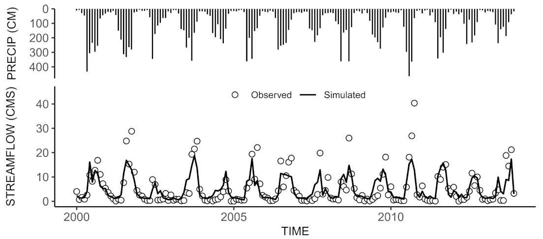
Overall, a good calibration of the proposed model was obtained when compared to the observed flow discharge at the outlet of the Huazuntlan River Watershed. Figure 7 shows the observed flow discharge and the best simulated flow signal after automatic calibration and validation procedures. The NSE value for the calibration period was 0.69, $R^2$ was 0.84, whereas PBIAS was 3.1%, which represent a good performance for monthly flow discharge calculations according to [44]. Similarly, the performance during the validation period NSE was 0.64, $R^2$ was 0.83, and PBIAS was 12.5%, which are in the range bracketing a good fit between the observed and simulated signals (see

Table 3. Observed vs simulated streamflow goodness of fit.

Period	NSE	${\mathit{R}}^2$	PBIAS
Calibration	0.69	0.84	3.1
Validation	0.64	0.83	12.5

). The mean, maximum, and minimum observed discharge for the calibration period were 5.28, 28.78, and 0.03 m${}^3$/s, respectively. The simulated flow showed a mean, maximum, and minimum of 5.12, 20.75, and 0.55 m${}^3$/s, respectively. It can be noticed that similar flow magnitudes were obtained between the predictions and the observations. However, minimum flow conditions were the slightly over-predicted by the model. During the model validation, the mean, maximum, and minimum observed discharge for the calibration period were 5.99, 40.35, and 0.04 m${}^3$/s, respectively, while during simulated conditions, the validation period showed mean, maximum, and minimum of 5.30, 17.33, and 0.90 m${}^3$/s, respectively. We can see that the mean discharge agreed well with its simulated counterpart. However, several peaks during both calibration and validation were not able to be captured by the model accurately. Similarly to the calibration period, the model slightly overestimated the base-flow conditions, especially for those months with low values of precipitation.

3.3. Hydrological Behavior of the Watershed

The SWAT model proposed in this study performed well and indicated a linear watershed hydrologic response as it presented a rapid response to rainfall events, except for storm events presented during the intense summer rainfall generally preceded by dry conditions. This linearity and rapid response of the watershed is attributed to the response to the subsurface lateral flow [45]. Evidence of this type of hydrologic behavior is accountable for the relatively high values of ALPHA_BF during the calibration period [46]. Although non-linearity response assumes that overland flow in steep mountainous catchments is the most significant contribution to the streamflow, surface run-off is unlikely to happen in forested hillslopes due to the high hydraulic conductivities of the soil, which is the case for the mainly forested Huazuntlan River Watershed. As a result, in the shallow soils found in the study area, a preferential flow mechanism is likely to occur within the watershed. This process is common to happen in mostly humid climate and forested watersheds [47] due to ephemeral and perennial pipes in the soil maintained mainly by subsurface flow and burrowing animals, respectively. This type of preferential flow is quite complex to explain and simulated and it is only possible to discuss by the statistical properties of parameters defining the movement of the subsurface in hydrological models. In addition, in SWAT models, the representation of the water table attributes and position tends to be inadequate. As a result, the parameters controlling shallow groundwater structure will have a large source of uncertainty associated with them [48]. A more discrete spatial representation of the aquifer characteristics and groundwater systems within sub-watersheds may increase the model accuracy.

The overall hydrologic response of the watershed showed that observed and simulated streamflow outputs presented similar phases and trends, as well as a reasonable match with the observed peaks during humid season (see Figure 7). However, significant deviations between the simulated and observed peaks were found. These deviations, present during high-intensity rainfall events, might be due to the precipitation heterogeneity within the watershed or the well-known curve number (CN) method limitations. The CN method does not considered neither the storm or precipitation duration and its intensity [49], which can limit the SWAT model to estimate the magnitude of the flow discharge peaks [50]. Regardless these limitations, the CN method slightly overestimated streamflow for some large rainfall events and showed some limitations to capture the peak during the high-intensity rainfall season. This peak mismatching, as previously mentioned, is present due to the spatial-temporal variability of the rainfall data, which was heterogeneous by nature. Additionally, peak discharges may be due to changes in land use influencing the hydrological phenomena of the direct run-off. In this study, a increase of 25% of the overall curve number was found during the calibration period. Although the calibration procedure produced a good performance, a more accurate representation of the CN may be obtained from a spatial and dynamic calibration of this parameter.

At large basins, the residence time plays an important role during calibration. These residence time refers to the average time that a certain amount of water travels through a defined river reach. In SWAT model, this variable is affected by the Mannign’s roughness coefficient, which by the definition influences the mean velocity of the flow traveling through streams. This roughness was homogeneously assumed in the proposed SWAT model, having a calibrated value of natural streams (∼0.06 [51]). Additionally, the hydraulic conductivity of the overall system of streams presented an average value of 476.15 mm/day, which represent a high transmissivity of water from the streams to the hillslope or vice versa, which is consisted with the high rates of lateral flow dominating the flow hydrograph. Overall, the annual average discharge from 2000 to 2013 were 5.49 and 5.17 m${}^3$/s for the measured and simulated data, respectively. These values and the performance metrics indicate that the model can be applied for further assessment of the hydrologic response under different land use scenarios. It is carefully noted, that some uncertainty is always introduced into a hydrologic model regardless the agreement between the simulated and observed signals [52]. The foretold uncertainties may arise from different sources, including the model conceptual structure, assumed initial conditions, observed input data, and selected calibration parameters. The latter have been discussed extensively and although 20 parameters were selected as the most significant, Duan et al. [52] suggested that more variables are needed for calibration purposes.

3.4. Hydropower Map

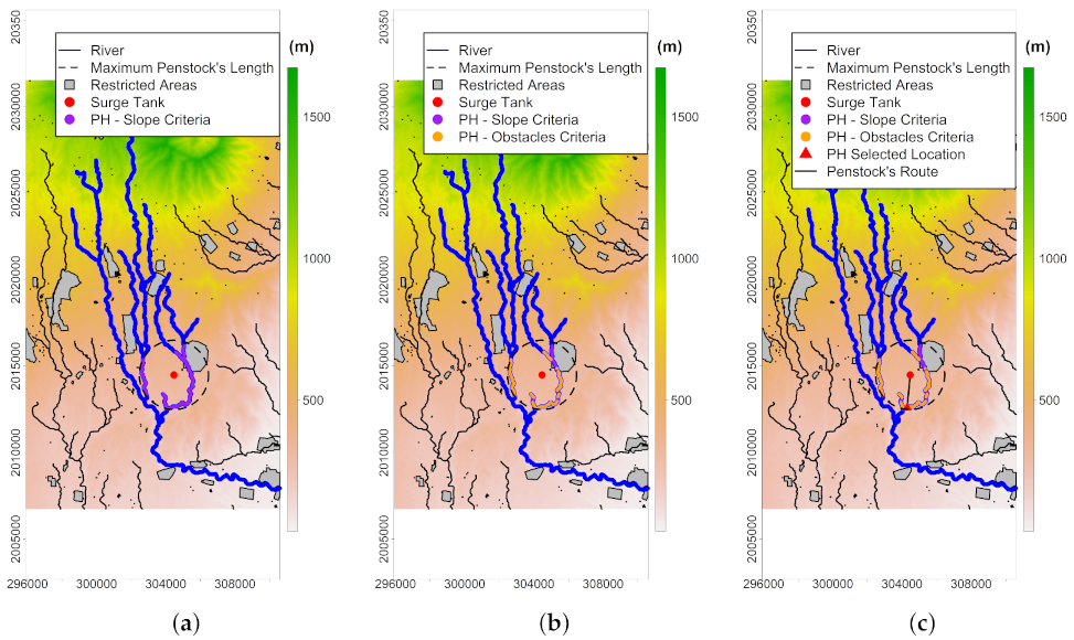
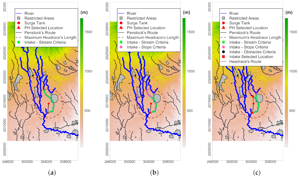
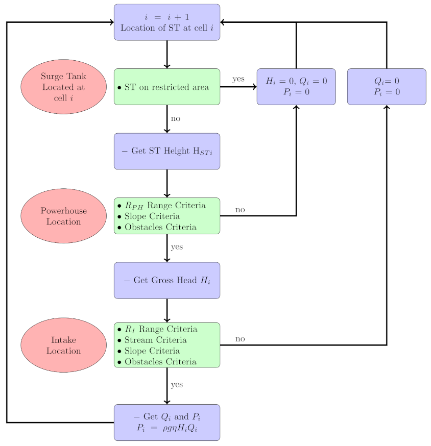
Hydropower maps were obtained by implementing the MSA according to the scheme of Figure 5 for different pairs of values $(R_{PH},R_I)$ representing the headrace’s and penstock’s maximum permissible lengths, respectively. Values of (100, 250, 500, 1000, 1500, 2000, 2500) m were used for $R_{PH}$ and $R_I$ to get a more comprehensive understanding of the interaction between both variables. Due to computing access limitations (i.e., HPC account expired), results for $(R_{PH},R_I)$ = (2500, 2500) m were not considered. As a result, only 48 simulations were analyzed. Potential sites include mountainous regions with steep geographies, as well as downstream places.

Figure 8 shows hydro-power maps for the three representative $(R_{PH},R_I)$ cases, $(250,2000)$, $(1000,2000)$ and $(2500,2000)$ m, where $R_I$ is a fixed value. For the sake of visualization, different scales were used. It can be observed that for all three maps, most of the values are close to zero. The main reason is that places far away from the river were not included within the $R_{PH}$ or the $R_I$ radius. For some other cases, it could be that obstacles were obstructing the headrace’s or the penstock’s path, or simply that the study site did not meet the requirements given by the model. Overall, the larger the $R_{PH}$ values, the more potential sites were found with higher hydro-power. Additionally, spatially speaking, a non-uniform hydro-power distribution was present on all maps. This behavior is due to an implicit balance between discharges Q and hydraulic heads H, which is required for hydro-power estimation according to Equation (1). This translates to flow discharges increasing from downstream to upstream (from north to south), and higher elevation gradients present more commonly at high elevations. For instance, when $(R_{PH},R_I)$ were (250, 2000) m, specifically Figure 8a, potential sites with hydro-power lower than 1500 kW tended to be located within the buffer created along flood plains of the river and dominated by $R_{PH}$. Locations with hydro-power higher than 1500 kW were mostly at the junction of the river’s main stem and tributaries and other downstream zones. Similarly, for Figure 8b,c, increments in hydro-power were due to the magnitude of $R_{PH}$. However, whereas the former showed the highest hydro-power values ranging from 1500 to 2500 kW over similar locations as shown in Figure 8a, the extension increased. Lastly, Figure 8c shows significant changes in potential locations for hydro-power generations, where the locations with the highest hydro-power (>2000 kW) were located downstream and all over the middle and top sections of the watershed. According to all this, it would be possible to select high potential sites without interfering with other high potential sites.

For fixed values of $R_{PH}$ and three representative values of $R_I$, Figure 9 shows cases $(2000,250)$, $(2000,1000)$ and $(2000,2500)$ m. Once again, different scales were used for each map for the sake of visualization. It can be seen that for the first scenario, there are fewer potential sites for low values of $R_I$ with the highest hydro-power close to the mouth of the river (Figure 9a). An increment in $R_I$ showed that hydro-power ranged from 500 to 2000 kW and was mostly located at the watershed’s headwaters. Additionally, a few locations with $HP>2000$ kW were at the junction of the main river and its tributaries and close the watershed’s outlet (Figure 9b). The last scenario with $R_{PH}=2000$ and $R_I=2500$ m showed a similar hydro-power distributions as in Figure 8c. However, potential locations with moderate hydro-power conditions $(1500<HP<2000)$ kW were located mainly over the middle and top sections of the watershed, whereas the highest hydro-power, $HP>2000$ kW, were still located at the river’s junction and near the mouth of the watershed (Figure 9c). Once again, it can be seen that high potential sites do not interfere with other high potential sites under this approach.

The MSA shares common criteria with other methodologies. Works such as [3,16,17] located the different components of the RoR scheme by fixing maximum distances between surge tank and powerhouse. Then, the head was maximized according to the given criteria. Nevertheless, in these works, hydro-power was assessed by first establishing the position of the weir along the river. Thereafter, the position of the surge tank is conditioned when included in the model. This limits the potential sites to locations along the river and at sub-basin levels. This MSA method, on the other hand, allows multiple potential sites over the entire study area or any raster region (e.g., Figure 8 and Figure 9).

3.5. $R_{PH}$ and $R_I$ Contributions

To observe the effect of the $R_{PH}$ and $R_I$ parameters,

Table 4. Mean HP[kW] for the 243 maximum values.

${\mathit{R}}_{\mathit{PH}}$/${\mathit{R}}_{\mathit{I}}$	100	250	500	1000	1500	2000	2500
100	103.8	305.9	505.9	676.7	804.5	995.2	1295.3
250	145.8	381.0	596.23	882.6	1189.6	1655.1	2077.3
500	264.7	479.6	756.2	1116.1	1337.9	1794.0	2549.2
1000	425.4	729.0	969.1	1378.9	1659.3	2511.1	3017.0
1500	562.1	1020.1	1301.9	1672.6	1897.9	2923.1	3341.3
2000	791.0	1281.5	1650.9	1972.1	2252.1	2973.4	3432.0
2500	754.5	1361.5	1734.6	2002.1	2351.3	3057.8	NA

shows the mean value for the 243 sites with the highest hydro-power. This amounts only to the 0.01% of the total simulated data. The mean values ranged from 103 to 3432 kW. It is important to highlight that considering the mean of all values (100% of the total data) would lead to wrong conclusions since there are plenty of locations with zero potential values. This study was only concerned about the sites with the highest potentials. For the HP values on Table 4, a multiple linear regression model with interaction effect was estimated as $P\sim R_{PH}+R_I+R_{PH}\times R_I$ with a 0.945 value for the $R^2$ correlation coefficient. The predictors $R_{PH}$, $R_I$ and $R_{PH}\times R_i$ were $0.355$, $0.654$, and $0.221\times {10}^{-3}$, respectively.

Table 5. Regression Model for the Mean HP[kW] for the 243 maximum values.

	Estimate	Std. Error	t-Stat	p-Value
(Intercept)	79.6	86.5	0.92	0.3625
$R_{PH}$	0.355	0.062	5.68	0.0000
$R_I$	0.654	0.062	10.47	0.0000
$R_{PH}$×$R_I$	0.000221	0.000048	4.62	0.0000

shows reasonable contribution of interaction term and the penstock’s length, whereas the strongest contribution to the hydro-power was due to the headrace’s maximum length with a significance level of 0.05. Namely, an increase in 100 m for $R_{PH}$ is associated with an increase in 35.456 + 0.0221 $R_I$ kW, meanwhile an increase in 100 m for $R_I$ is associated with an increase in 65.379 + 0.0221 $R_{PH}$ kW. The interception term shows to be not significant in the regression equation with $p=0.3625$ since neither $R_{PH}$ or $R_I$ can be set to zero as this combination makes an irrational arrangement in a hydro-power generation system.

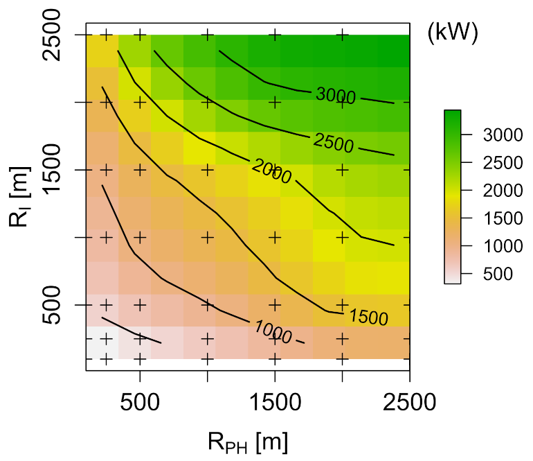
Figure 10 describes the parametric space for $R_{PH}$ and $R_I$ through a contour plot for the hydro-power conditions shown in Table 4. The interpolation was performed using a cubic spline. A thorough analysis of the level plot supports the same conclusion as the one derived from the regression equation. Small increments in $R_I$ produce a significant increment in hydro-power, especially for high values of $R_{PH}$. Besides, this description of the two variables involved in hydro-power production allows the observation of all possible system arrangements, which is an advantage derived from the use of raster information. 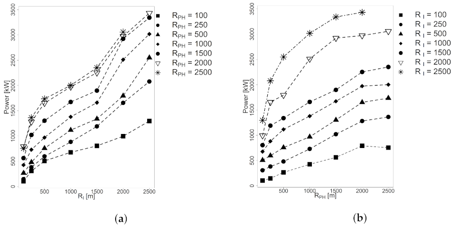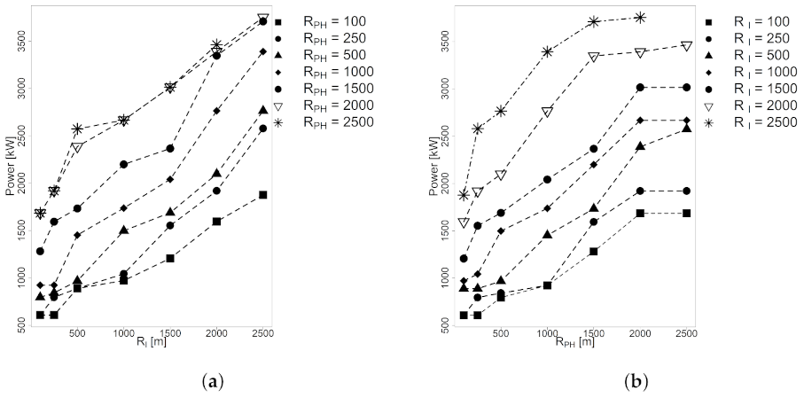Figure 11a plots the mean HP against the $R_I$ by fixing the $R_{PH}$ for different values. It shows a linear increment of the power as the $R_I$ length increases. Moreover, when $R_I$ takes values from 1500 to 2000 m, there is a significant increment in power for $R_{PH}$ values higher than 1000 m. The lines $R_{PH}=2000$ m and $R_{PH}=2500$ m show no significant difference for any $R_I$ value. On the other hand, Figure 11b plots mean HP against the $R_{PH}$ by fixing the $R_I$ for different values. There was an asymptotic trend for $R_{PH}$ values higher than 1500 observed for all $R_I$ values. This suggested $R_{PH}$ values within the range $(1000,1500)$ m behave as a threshold for this parameter, as no significant gains in power were obtained when increasing. The lines $R_I=2000$ m and $R_I=2500$ m show no significant difference for low $R_{PH}$ values.

Table 6. Maximum HP[kW] values.

${\mathit{R}}_{\mathit{PH}}$/${\mathit{R}}_{\mathit{I}}$	100	250	500	1000	1500	2000	2500
100	608.2	608.2	889.3	971.7	1206.1	1595.2	1875.6
250	608.2	795.6	889.3	1042.6	1552.6	1919.6	2577.5
500	795.3	842.1	968.7	1497.7	1688.6	2098.3	2764.6
1000	923.1	923.2	1452.3	1736.9	2041.1	2764.6	3390.2
1500	1280.9	1593.2	1733.4	2198.9	2365.8	3346.2	3707.9
2000	1684.8	1920.0	2386.9	2666.7	3013.9	3390.2	3751.9
2500	1684.8	1920.0	2573.1	2666.7	3013.9	3462.0	NA

indicates the maximum hydro-power for each run. Maximum HP values range from 608 to 3752 kW for the $(100,100)$ m and $(2000,2500)$ m cases, respectively. One could see that this case represented the topmost hydro-power condition, whereas the previous case includes a representative selection of the maxima HP (e.g., 0.01% of the entire raster database). A multiple linear regression model with form $P\sim R_{PH}+R_I$ was adjusted to explained the variability of the maximum hydro-power as a function of $R_{PH}$ and $R_I$. The $R^2$ value was equal to 0.950, which means HP depends linearly on the penstock’s and the headrace’s length. The predictor’s values were 0.714 and 0.823 for $R_{PH}$ and $R_I$, respectively (

Table 7. Linear Regression Model for the maximum HP$\left[kW\right]$ values.

	Estimate	Std. Error	t-Stat	p-Value
(Intercept)	225.4	65.1	3.46	0.0012
$R_{PH}$	0.714	0.036	19.66	0.0000
$R_I$	0.823	0.036	22.66	0.0000

). Although both variables had a significant effect on the maximum HP, headrace’s length $R_I$ had a slightly stronger effect ($p=0.0000$). Once again, the interception term played an important effect on the maximum HP when considering a complete hydro-power generation system. However, it would be meaningless to consider its effect on HP by itself.

Figure 12a shows a linear increment of the hydro-power as $R_I$ increases, and a significant increment when increasing from 1500 to 2000 m for $R_{PH}$ values greater than 1000 m. Once again, the lines corresponding to $R_{PH}=2000$ m and $R_{PH}=2500$ had no significant difference for any $R_I$ value. Additionally, for small $R_I$ values within the range $(100,500)$ m some hydro-power lines for different $R_{PH}$ values intercept each other, that is the case of $(100,500)$ m and $(250,500)$ m. There is no guarantee that by increasing $R_{PH}$ or $R_I$ by a relatively small amount, HP value will increase. This is because the $R_{PH}$ and $R_I$ values stand for the maximum permissible penstock’s and headrace’s length, respectively, but in general, the values for both lengths are lower than permissible ones.

On the other hand, Figure 12b plots maximum HP against $R_{PH}$ for different $R_I$ values. No significant increments were observed for $R_{PH}$ greater than 2000 m for all $R_I$ values. There are also cases, where where hydro-power lines intercept, or closely intercept each other. That is the case of $(2500,2000)$ m and $(2500,1500)$ m. Nevertheless, compared with Figure 12a there are fewer cases since the increment on $R_I$ has a stronger increment on the HP.

Results indicated that according the MSA the headrace’s length, $R_I$, plays an important role on HP assessment and has to be taken into account to generate a more effective hydro-power generation system. However, general studies for hydro-power assessment models mainly focus on the penstock and ignore the headrace contribution in their models [17,22,53].

3.6. Considerations

Although the raster representation associates a hydro-power potential to every position, it does not mean that all sites can be used at the same time, as there could be interference between potential RoR projects. In fact, each cell of the hydro-power map contains additional information such as the powerhouse locations, the intake, the surge tank, and the headrace’s and penstock’s route, the flow discharge as well as the gross head. Therefore, when one selects a location for potential use, not only consider that single location but the complete facilities and a segment of the river, which restricts, in consequence, the selection of other potential locations. Additionally to these considerations, working with a raster representation carries advantages for further data processing and analysis. In fact, implementations such as turbine selection or MCDM analysis becomes a straightforward task [28,54]. For instance, Figure 13 presents a simple scheme of 5 non-overlapping projects by considering the $R_{PH}=1500$ m and $R_I=2000$ m. The extent was divided in five equally sized horizontal rectangles from east to west. As a result of the approach used in this study, the highest hydro-power values were 492.61, 1355.98, 1408.47, 2000.90, and 3346.18 kW for sites located from top to bottom of the image or downstream direction. The highest potential location among all the trials is shown in black. More complex optimization procedures could be implemented [22,55] as the MSA procedure was designed for further applications and research. That being said, the MSA methodology can be improved or extended without compromising it. An important improvement would be modeling more complex routes for the headrace and the pentsock by incorporating variables such as land use, watershed geomorphology, head losses, and economic costs. It could also be possible to integrate the different scenarios for the different parameters $R_{PH}$ and $R_I$, all in a single raster, in order to provide enough information, and make it open and accessible for the community.

4. Conclusions

The present work developed the MSA methodology devoted to obtain hydro-power potential maps distributed on a rectangular grid for a run of river scheme. The study area was the Huazuntlan River Watershed at the Tuxtlas Mountains, Veracruz, Mexico. The proposed method calculates the hydro-power on each location of the map where the position of the surge tank is established. Then, the position of the powerhouse and the intake are determined in the respective order by using the topographic and environmental factors, along with the SWAT model to obtain the watershed hydrologic response.

Hydro-power maps, were generated by controlling the penstock’s and headrace’s maximum permissible lengths $(R_{PH}$,$R_I)$. The regression model showed the parameter $R_I$ had the major effect on the hydro-power estimation, followed by $R_{PH}$ and, lastly, the interaction effect with a fair contribution. In a more realistic condition, where hydraulic losses are considered, the impact of $R_I$ would be even greater than $R_{PH}$ on the hydro-power generation. The selection of $R_{PH}=$ 1500 m and $R_I=2000$ m yield an $HP=3350$ kW. This scenario behaves as a threshold condition since no significant gains were obtained after increasing either penstock’s or headrace’s maximum lengths.

Overall, the maps presented a non-uniform hydro-power distribution with possible potential sites located at downstream, middle, and headwaters area of the watershed. Moderate hydro-power values are mostly at the junction of the river’s main stem and tributaries and other downstream areas. This makes the MSA procedure suitable for a sequence of RoR project along the different sites of the watershed.

The SWAT model used here provided an effective tool to estimate streamflow conditions for the different annual seasons in the study. The model shows an overall efficiency of 0.67, which is considered a good performance for various hydrological models (i.e., $0.65$ < NSE < $0.75$). However, the MSA method does not limit the use of other hydrological models and is flexible to higher time increments.

Although the MSA method assumed penstock’s and headrace’s routes as straight lines, and only gross hydro-power was calculated with no consideration of losses and ecological flows, the base methodology can be easily enriched. For instance, the straight-line assumption of the headrace and the penstock could be relaxed, and the model could incorporate more variables such as land use, watershed geomorphology, head losses, and economic costs. Additionally, improvements can include the hydrological modeling temporal and spatial resolution, and the implementation of MCDM analysis.

The central idea of MSA the developed methodology is relatively simple to apply, and, therefore, replicable. This approach involves elementary geoprocesses, such as searching extreme values in raster maps variables, intersecting different geometries, calculating distances, among others. However, these basic calculations can take seconds to minutes, translating into long computation times for large study areas. For this, one needs high-performance computing (HPC) equipment or reduce the number of pixels by choosing smaller areas or with lower resolution and performing the calculations in parallel. Furthermore, the results found through this method will be sensitive to how it is modeled. Namely, the MSA is sensitive to define the headrace and the penstock routes, the criteria for the location of the turbines and the intake, and at the same time as the hydrological model used.

References

1. Kosa, P.; Kulworawanichpong, T.; Srivoramas, R.; Chinkulkijniwat, A.; Horpibulsuk, S.; Teaumroong, N. The potential micro-hydropower projects in Nakhon Ratchasima province, Thailand. Renew. Energy 2011, 36, 1133–1137. [Google Scholar] [CrossRef]
2. Okot, D.K. Review of small hydropower technology. Renew. Sustain. Energy Rev. 2013, 26, 515–520. [Google Scholar] [CrossRef]
3. Rojanamon, P.; Chaisomphob, T.; Bureekul, T. Application of geographical information system to site selection of small run-of-river hydropower project by considering engineering/economic/environmental criteria and social impact. Renew. Sustain. Energy Rev. 2009, 13, 2336–2348. [Google Scholar] [CrossRef]
4. EVE. Ente Vasco de la Energía (EVE). Available online: https://www.eve.eus/Conoce-la-Energia/Multimedia/Infografias/La-energia-minihidraulica?lang=es-es/ (accessed on 4 February 2021).
5. Zaidi, A.Z.; Khan, M. Identifying high potential locations for run-of-the-river hydroelectric power plants using GIS and digital elevation models. Renew. Sustain. Energy Rev. 2018, 89, 106–116. [Google Scholar] [CrossRef]
6. Tahri, M.; Hakdaoui, M.; Maanan, M. The evaluation of solar farm locations applying Geographic Information System and Multi-Criteria Decision-Making methods: Case study in southern Morocco. Renew. Sustain. Energy Rev. 2015, 51, 1354–1362. [Google Scholar] [CrossRef]
7. Firozjaei, M.K.; Nematollahi, O.; Mijani, N.; Shorabeh, S.N.; Firozjaei, H.K.; Toomanian, A. An integrated GIS-based Ordered Weighted Averaging analysis for solar energy evaluation in Iran: Current conditions and future planning. Renew. Energy 2019, 136, 1130–1146. [Google Scholar] [CrossRef]
8. Mancini, F.; Nastasi, B. Solar energy data analytics: PV deployment and land use. Energies 2020, 13, 417. [Google Scholar] [CrossRef] [Green Version]
9. Noorollahi, Y.; Yousefi, H.; Mohammadi, M. Multi-criteria decision support system for wind farm site selection using GIS. Sustain. Energy Technol. Assess. 2016, 13, 38–50. [Google Scholar] [CrossRef]
10. Mahdy, M.; Bahaj, A.S. Multi criteria decision analysis for offshore wind energy potential in Egypt. Renew. Energy 2018, 13, 278–289. [Google Scholar] [CrossRef]
11. Spyridonidou, S.; Sismani, G.; Loukogeorgaki, E.; Vagiona, D.G.; Ulanovsky, H.; Madar, D. Sustainable Spatial Energy Planning of Large-Scale Wind and PV Farms in Israel: A Collaborative and Participatory Planning Approach. Energies 2021, 3, 551. [Google Scholar] [CrossRef]
12. Natarajan, K.; Latva-Käyrä, P.; Zyadin, A.; Pelkonen, P. New methodological approach for biomass resource assessment in India using GIS application and land use/land cover (LULC) maps. Renew. Sustain. Energy Rev. 2016, 63, 256–268. [Google Scholar] [CrossRef]
13. Jeong, J.S.; Ramírez-Gómez, Á. A multicriteria GIS-based assessment to optimize biomass facility sites with parallel environment—A case study in Spain. Energies 2017, 10, 2095. [Google Scholar] [CrossRef] [Green Version]
14. Zyadin, A.; Natarajan, K.; Latva-Käyrä, P.; Igliński, B.; Iglińska, A.; Trishkin, M.; Pelkonen, P.; Pappinen, A. Estimation of surplus biomass potential in southern and central Poland using GIS applications. Renew. Sustain. Energy Rev. 2018, 89, 204–215. [Google Scholar] [CrossRef]
15. Sánchez-Lozano, J.M.; Teruel-Solano, J.; Soto-Elvira, P.L.; García-Cascales, M.S. Geographical Information Systems (GIS) and Multi-Criteria Decision Making (MCDM) methods for the evaluation of solar farms locations: Case study in south-eastern Spain. Renew. Sustain. Energy Rev. 2013, 24, 544–556. [Google Scholar] [CrossRef]
16. Larentis, D.G.; Collischonn, W.; Olivera, F.; Tucci, C.E. Gis-based procedures for hydropower potential spotting. Energy 2010, 35, 4237–4243. [Google Scholar] [CrossRef]
17. Moiz, A.; Kawasaki, A.; Koike, T.; Shrestha, M. A systematic decision support tool for robust hydropower site selection in poorly gauged basins. Appl. Energy 2018, 224, 309–321. [Google Scholar] [CrossRef]
18. Kusre, B.C.; Baruah, D.C.; Bordoloi, P.K.; Patra, S.C. Assessment of hydropower potential using GIS and hydrological modeling technique in Kopili River basin in Assam (India). Appl. Energy 2010, 224, 298–309. [Google Scholar] [CrossRef]
19. Cuya, D.G.P.; Brandimarte, L.; Popescu, I.; Alterach, J.; Peviani, M. A GIS-based assessment of maximum potential hydropower production in La Plata basin under global changes. Renew. Energy 2013, 50, 103–114. [Google Scholar] [CrossRef]
20. Fujii, M.; Tanabe, S.; Yamada, M.; Mishima, T.; Sawadate, T.; Ohsawa, S. Assessment of the potential for developing mini/micro hydropower: A case study in Beppu City, Japan. J. Hydrol. Reg. Stud. 2017, 11, 107–116. [Google Scholar] [CrossRef] [Green Version]
21. Bayazıt, Y.; Bakış, R.; Koç, C. An investigation of small scale hydropower plants using the geographic information system. Renew. Sustain. Energy Rev. 2017, 67, 289–294. [Google Scholar] [CrossRef]
22. Ibrahim, M.; Imam, Y.; Ghanem, A. Optimal Planning and Design of Run-of-river Hydroelectric Power Projects. Renew. Energy 2019, 141, 858–873. [Google Scholar] [CrossRef]
23. Abdelhady, H.U.; Imam, Y.E.; Shawwash, Z.; Ghanem, A. Parallelized Bi-level optimization model with continuous search domain for selection of run-of-river hydropower projects. Renew. Energy 2021, 167, 116–131. [Google Scholar] [CrossRef]
24. Yi, C.S.; Lee, J.H.; Shim, M.P. Site location analysis for small hydropower using geo-spatial information system. Renew. Energy 2010, 35, 852–861. [Google Scholar] [CrossRef]
25. Zapata-Sierra, A.J.; Manzano-Agugliaro, F. Proposed methodology for evaluation of small hydropower sustainability in a Mediterranean climate. J. Clean. Prod. 2019, 214, 717–729. [Google Scholar] [CrossRef]
26. Sammartano, V.; Liuzzo, L.; Freni, G. Identification of potential locations for run-of-river hydropower plants using a GIS-based procedure. Energies 2019, 12, 3446. [Google Scholar] [CrossRef] [Green Version]
27. Wegner, N.; Mercante, E.; de Souza Mendes, I.; Ganascini, D.; Correa, M.M.; Maggi, M.F.; Boas, M.A.V.; Wrublack, S.C.; Siqueira, J.A.C. Hydro energy potential considering environmental variables and water availability in Paraná Hydrographic Basin 3. J. Hydrol. 2020, 580, 124–183. [Google Scholar] [CrossRef]
28. Williamson, S.J.; Stark, B.H.; Booker, J.D. Low head pico hydro turbine selection using a multi-criteria analysis. Renew. Energy 2014, 61, 43–50. [Google Scholar] [CrossRef]
29. R Core Team. R: A Language and Environment for Statistical Computing; R Foundation for Statistical Computing: Vienna, Austria, 2020. [Google Scholar]
30. Arnold, J.G.; Moriasi, D.N.; Gassman, P.W.; Abbaspour, K.C.; White, M.J.; Srinivasan, R.; Santhi, C.; Harmel, R.D.; Van Griensven, A.; Van Liew, M.W.; et al. SWAT: Model use, calibration, and validation. Trans. ASABE 2012, 55, 1491–1508. [Google Scholar] [CrossRef]
31. Arnold, J.G.; Srinivasan, R.; Muttiah, R.S.; Williams, J.R. Large area hydrologic modeling and assessment part I: Model development 1. J. Am. Water Resour. Assoc. 1998, 34, 73–89. [Google Scholar] [CrossRef]
32. Gassman, P.W.; Reyes, M.R.; Green, C.H.; Arnold, J.G. The soil and water assessment tool: Historical development, applications, and future research directions. Trans. ASABE 2007, 50, 1211–1250. [Google Scholar] [CrossRef] [Green Version]
33. Saha, S.; Moorthi, S.; Wu, X.; Wang, J.; Nadiga, S.; Tripp, P.; Behringer, D.; Hou, Y.T.; Chuang, H.Y.; Iredell, M. The NCEP climate forecast system version 2. J. Clim. 2014, 27, 2185–2208. [Google Scholar] [CrossRef]
34. Jarvis, A.; Reuter, H.I.; Nelson, A.; Guevara, E. Hole-Filled SRTM for the Globe Version 4, Available from the CGIAR-CSI SRTM 90m Database. 2008. Available online: https://www.researchgate.net/publication/225091464_Hole-filled_SRTM_for_the_globe_version_3_from_the_CGIAR-CSI_SRTM_90m_database (accessed on 19 May 2021).
35. Livneh, B.; Bohn, T.J.; Pierce, D.W.; Munoz-Arriola, F.; Nijssen, B.; Vose, R.; Cayan, D.R.; Brekke, L. A spatially comprehensive, hydrometeorological data set for Mexico, the US, and Southern Canada 1950–2013. Sci. Data 2015, 2, 1–12. [Google Scholar] [CrossRef]
36. FAO; IIASA; ISRIC; ISSCAS. JRC: Harmonized World Soil Database (Version 1.2); FAO: Rome, Italy; IIASA: Laxenburg, Austria, 2012. [Google Scholar]
37. CONAGUA. Banco Nacional de Datos de Aguas Superficiales. Gerencia de Aguas Superficiales e Ingenieria de Rios, Comision Nacional del Agua, Mexico. 2017. Available online: https://app.conagua.gob.mx/bandas/ (accessed on 16 September 2020).
38. Abbaspour, K.C.; Vaghefi, S.A.; Yang, H.; Srinivasan, R. Global soil, landuse, evapotranspiration, historical and future weather databases for SWAT Application. Sci. Data 2019, 6, 1–11. [Google Scholar] [CrossRef] [Green Version]
39. Abbaspour, K.C.; Yang, J.; Reichert, P.; Vejdani, M.; Haghighat, S.; Srinivasan, R. SWAT-CUP, SWAT Calibration and Uncertainty Programs; Eawag-Swiss Federal Institute of Aquatic Science and Technology: Duebendorf, Switzerland, 2011; p. 93. [Google Scholar]
40. Abbaspour, K.C.; Johnson, C.A.; Van Genuchten, M.T. Estimating uncertain flow and transport parameters using a sequential uncertainty fitting procedure. Vadose Zone J. 2004, 3, 1340–1352. [Google Scholar] [CrossRef]
41. Abbaspour, K.C.; Yang, J.; Maximov, I.; Siber, R.; Bogner, K.; Mieleitner, J.; Zobrist, J.; Srinivasan, R. Modelling hydrology and water quality in the pre-alpine/alpine Thur watershed using SWAT. J. Hydrol. 2007, 333, 413–430. [Google Scholar] [CrossRef]
42. Abbaspour, K.C.; Yang, J.; Maximov, I.; Siber, R.; Bogner, K.; Mieleitner, J.; Zobrist, J. Calibration and uncertainty issues of a hydrological model (SWAT) applied to West Africa. Adv. Geosci. 2006, 9, 137–143. [Google Scholar]
43. Abbaspour, K.C.; Rouholahnejad, E.; Vaghefi, S.; Srinivasan, R.; Yang, H.; Kløve, B. A continental-scale hydrology and water quality model for Europe: Calibration and uncertainty of a high-resolution large-scale SWAT model. J. Hydrol. 2015, 524, 733–752. [Google Scholar] [CrossRef] [Green Version]
44. Moriasi, D.N.; Arnold, J.G.; Van Liew, M.W.; Bingner, R.L.; Harmel, R.D.; Veith, T.L. Model evaluation guidelines for systematic quantification of accuracy in watershed simulations. Trans. ASABE 2007, 50, 885–900. [Google Scholar] [CrossRef]
45. Loukas, A.; Quick, M.C. Hydrologic behaviour of a mountainous watershed. Can. J. Civ. Eng. 1993, 20. [Google Scholar] [CrossRef]
46. Jang, W.S.; Engel, B.; Ryu, J. Efficient flow calibration method for accurate estimation of base-flow using a watershed scale hydrological model (SWAT). Ecol. Eng. 2018, 125, 50–67. [Google Scholar] [CrossRef]
47. Tanaka, T.; Yasuhara, M.; Sakai, H.; Marui, A. The Hachioji experimental basin study—storm runoff processes and the mechanism of its generation. J. Hydrol. 1998, 102, 139–164. [Google Scholar] [CrossRef]
48. Mapes, K.L.; Pricope, N.G. Evaluating SWAT model performance for runoff, percolation, and sediment loss estimation in low-gradient watersheds of the Atlantic coastal plain. Hydrology 2020, 7, 21. [Google Scholar] [CrossRef] [Green Version]
49. Nie, W.; Yuan, Y.; Kepner, W.; Nash, M.S.; Jackson, M.; Erickson, C. Assessing impacts of Landuse and Landcover changes on hydrology for the upper San Pedro watershed. J. Hydrol. 2011, 407, 105–114. [Google Scholar] [CrossRef]
50. King, K.W.; Arnold, J.G.; Bingner, R.L. Comparison of Green-Ampt and curve number methods on Goodwin Creek watershed using SWAT. Trans. ASABE 1999, 42, 919. [Google Scholar] [CrossRef]
51. Sturm, T.W. Open Channel Hydraulics; McGraw-Hill: New York, NY, USA, 2001; pp. 115–118. [Google Scholar]
52. Duan, W.; He, B.; Takara, K.; Luo, P.; Nover, D.; Hu, M. Impacts of climate change on the hydro-climatology of the upper Ishikari river basin, Japan. Environ. Earth Sci. 2017, 76, 1–16. [Google Scholar] [CrossRef]
53. Trelles-Jasso, A. Evaluation of Small Hydro Power Potential in Three River Basins of Mexico; Mexican Institute of Water Technology (IMTA): Jiutepec, Mexico, 2009. [Google Scholar]
54. Otuagoma, S.O. Turbine Selection Criteria for Small Hydropower Development–The River Ethiope Experience. Int. J. Eng. Res. Technol. 2016, 2, 34–40. [Google Scholar]
55. Yildiz, V.; Vrugt, J.A. A toolbox for the optimal design of run-of-river hydropower plants. J. Hydrol. 2019, 111, 134–152. [Google Scholar] [CrossRef] [Green Version]
Figure 1. Run of River Scheme: (1) Diversion Weir, (2) Intake, (3) Headrace, (4) Surge Tank, (5) Penstock, (6) Powerhouse, (7) Tail Race [4].
Energies 14 03095 g001
Figure 2. Run of River scheme includes the intake, the surge tank and the powerhouse.
Energies 14 03095 g002
Figure 3. Powerhouse site selection process. (a) Slope Criteria (b) Obstacles Criteria (c) Maximum gross head. Maximum permissible penstock’s length for example is set to RPH = 2000 m.
Energies 14 03095 g003
Figure 4. Intake site selection process. (a) Stream criteria (b) Slope criteria (c) Obstacles criteria. Maximum permissible headrace’s length for example is set to RI = 3000 m.
Energies 14 03095 g004
Figure 5. Mesh sweeping approach (MSA) methodology flow diagram.
Energies 14 03095 g005
Figure 6. Huazuntlan River Watershed: left: digital elevation model; right: land use distribution. Units in meters.
Energies 14 03095 g006
Figure 7. Huazuntlan River Watershed hydrologic response. Top: monthly precipitation; Bottom: observed streamflow (circles) and simulate streamflow (solid line).
Energies 14 03095 g007
Figure 8. Hydropower maps for fixed maximum headrace’s length R I = 2000 m.
Energies 14 03095 g008
Figure 9. Hydropower maps for fixed maximum penstock’s length R P H = 2000 m.
Energies 14 03095 g009
Figure 10. Mean HP for the 243 maximum values.
Energies 14 03095 g010
Figure 11. Power as function of RI and RPH for mean of 243 maximum values. (a) Fixed RPH value (b) Fixed RI value.
Energies 14 03095 g011
Figure 12. Power as function of RI and RPH for maximum HP values. (a) Fixed RPH value (b) Fixed RI value.
Energies 14 03095 g012
Figure 13. Hydropower map for R P H = 1500 m and R I = 2000 m, presenting 5 non-overlapping projects.
Energies 14 03095 g013