Impact of Chemistry–Turbulence Interaction Modeling Approach on the CFD Simulations of Entrained Flow Coal Gasification

Abstract

This paper examines the impact of different chemistry–turbulence interaction approaches on the accuracy of simulations of coal gasification in entrained flow reactors. Infinitely fast chemistry is compared with the eddy dissipation concept considering the influence of turbulence on chemical reactions. Additionally, ideal plug flow reactor study and perfectly stirred reactor study are carried out to estimate the accuracy of chosen simplified chemical kinetic schemes in comparison with two detailed mechanisms. The most accurate global approach and the detailed one are further implemented in the computational fluid dynamics (CFD) code. Special attention is paid to the water–gas shift reaction, which is found to have the key impact on the final gas composition. Three different reactors are examined: a pilot-scale Mitsubishi Heavy Industries reactor, a laboratory-scale reactor at Brigham Young University and a Conoco-Philips E-gas reactor. The aim of this research was to assess the impact of gas phase reaction model accuracy on simulations of the entrained flow gasification process. The investigation covers the following issues: impact of the choice of gas phase kinetic reactions mechanism as well as influence of the turbulence–chemistry interaction model. The advanced turbulence–chemistry models with the complex kinetic mechanisms showed the best agreement with the experimental data.

1. Introduction

Gasification is a way of treating carbon-based feedstock to enhance its quality and value [1]. Solid fuels with low calorific value can be successfully converted into a high-quality fuel to be further used in various industry sectors [2]. The process consists in the thermochemical conversion of a carbon-based solid fuel within different mediums (O₂, H₂O, CO₂, and air), resulting in a combustible gas product consisting mostly of CO and H₂, which is a synthesis gas.

Gasification consists of such key stages as drying, devolatilization, partial oxidation/combustion, and gasification/reduction, whereby it is a very complicated process involving many overlapping reactions in both gas and solid phases, depending on the process parameters, such as temperature, pressure or fuel properties.

The reactive flow as well as gas phase kinetic reactions have a significant impact on the final composition of the syngas. The ability to properly simulate these processes can have a significant impact on the reactor and process design through considering temperature as well residence time of the reactants.

Therefore, in order to achieve high process efficiency in various operating conditions, proper optimization needs to be performed. Unfortunately, the use of experimental techniques for this purpose can be very challenging or even inviable, especially in the case of large-scale reactors. Computational fluid dynamics (CFD) has gained significant attention recently [3,4,5,6,7,8]. CFD modeling tools incorporate specific algorithms to describe such processes as moisture evaporation, devolatilization or char conversion. CFD has proved to be an efficient and convenient method for optimizing, designing and retrofitting reactors.

Recently, Mularski et al. [9] carried out a comprehensive review of the latest trends in the CFD modeling of entrained flow coal gasification. The authors concluded that while there was abundant literature on devolatilization and char conversion phenomena, there was scarce information concerning the impact of the gas phase on entrained flow coal gasification. Unlike in conventional combustion, where infinitely fast chemistry is generally assumed, in the case of gasification there is an extended reacting flow region with lower temperatures where chemical reaction rates are comparable to turbulent mixing rates. Therefore, the interaction between the turbulent effects and the reaction chemistry needs to be accurately described.

Park et al. [10] assessed the direct influence of turbulence–chemistry interaction (TCI) models (the eddy dissipation model and the finite-rate/eddy dissipation model) on the gasification process. They found the impact of gas phase reactions to be negligible when the Damköhler (Da) number was greater than 1. In such conditions the mixing rate was far a more dominant factor than the chemical reactions.

Vascellari et al. [11] examined the impact of the turbulence–chemical interaction in the gas phase on moderate or intense low-oxygen dilution (MILD) coal combustion. The eddy dissipation concept with the detailed GRI-Mech mechanism proved to be the most accurate gas phase modeling combination.

Modliński and Hardy [12] studied different gas phase reaction mechanisms in pulverized coal combustion (PCC). The mechanisms were found to have a substantial effect on gas composition and temperature distribution.

Wang et al. [13] optimized global reaction mechanisms under MILD combustion in a plug flow reactor and in a hot co-flow combustion system in CFD. The study showed a huge impact of kinetics in the examined conditions.

The main objectives of this research were (1) to compare two fundamental gas phase modeling approaches the eddy dissipation model (infinitely fast chemistry assumption) and the eddy dissipation concept (taking into consideration chemical kinetics), (2) to compare different gas phase global combustion mechanisms with two detailed mechanisms—GRI-Mech [14] and CRECK [15,16] in gasification conditions in plug flow and perfectly stirred reactor computations and to implement the most accurate one into CFD, (3) to carry out a CFD analysis of the gas phase combustion mechanisms and turbulence–chemistry interaction approaches and a validation study for the three different gasification reactors:

• a 0.5 tons/day laboratory-scale, one-stage reactor at Brigham Young University [17];
• a 200 tons/day, pilot-scale, two-stage Mitsubishi Heavy Industries reactor [18];
• a 2400 tons/day, two-stage Conoco-Philips E-gas reactor [19];

and (4) to carry out a detailed analysis of the impact of the water–gas shift reaction on the final gas composition.

The novelty of this paper consists in examining the impact of different chemical reaction mechanisms and turbulence–chemistry interaction approaches strictly in gasification under different operating reactor conditions on gas composition and temperature distribution.

2. Entrained Flow Gasification Mathematical Models

The commercial CFD software ANSYS Fluent [20] was applied to investigate entrained flow coal gasification. The Reynolds averaged Navier–Stokes (RANS) equations are solved using the finite-volume discretization approach. The semi-implicit method for pressure linked equations (SIMPLE) [21] algorithm is used for pressure–velocity coupling. Second-order schemes are applied for spatial discretization.

The Eulerian approach is used to model the gas phase. The Lagrangian formulation is used to calculate discrete phase trajectories, whereas the coupling between the phases is introduced through the particle sources of the Eulerian gas phase equations [22]. Simulations are run for the following processes inside the reactor: turbulent flow, moisture evaporation, devolatilization, gas phase, char conversion, radiative transport and particle transport. In the particle transport model, the mass flow of coal parcels is represented by a specific number of trajectories which stand for a much larger number of actual particles. A summary of the models applied to the reactors is presented in

Table 1. Summary of applied modeling approaches.

Models	BYU Gasifier	MHI Gasifier	E-Gas Gasifier
Devolatilization:	Chemical percolation devolatilization model (CPD) [26,27,28] Functional-group, depolymerization, vaporization, cross-linking model (FG-DVC) [29]	Single-step first-order reaction model (SFOR) [30,31,32,33] Functional-group, depolymerization, vaporization, cross-linking model (FG-DVC)	Competing two-step reaction model (C2SM) [32] Functional-group, depolymerization, vaporization, cross-linking model (FG-DVC)
Gas phase:	Global reaction approach with finite-rate/eddy dissipation model Global reaction approach with eddy dissipation concept Detailed GRI-Mech mechanism with eddy dissipation concept
Char conversion:	Multiple surface reaction model [25]
Turbulence:	Realizable k-ε model [23]
Radiation:	Discrete ordinate method [20]
Gas absorption coefficient:	Weighted sum of gray gas model [20]
Pressure-velocity coupling	Semi-implicit method for pressure linked equations (SIMPLE) [21]

. Turbulence is modelled with the realizable k-ε approach [23]. The turbulent particle dispersion is considered with a stochastic tracking model [24]. Radiation is modelled with the discrete ordinate method [20]. Char conversion is modelled with the CFD-built-in implicit approach [20,25]—the multiple surface reaction model. The weighted-sum of gray gas (WSGG) model [20] is used to calculate the gas absorption coefficient. The devolatilization and gas phase modeling approaches are presented in separate sub-sections.

Devolatilization

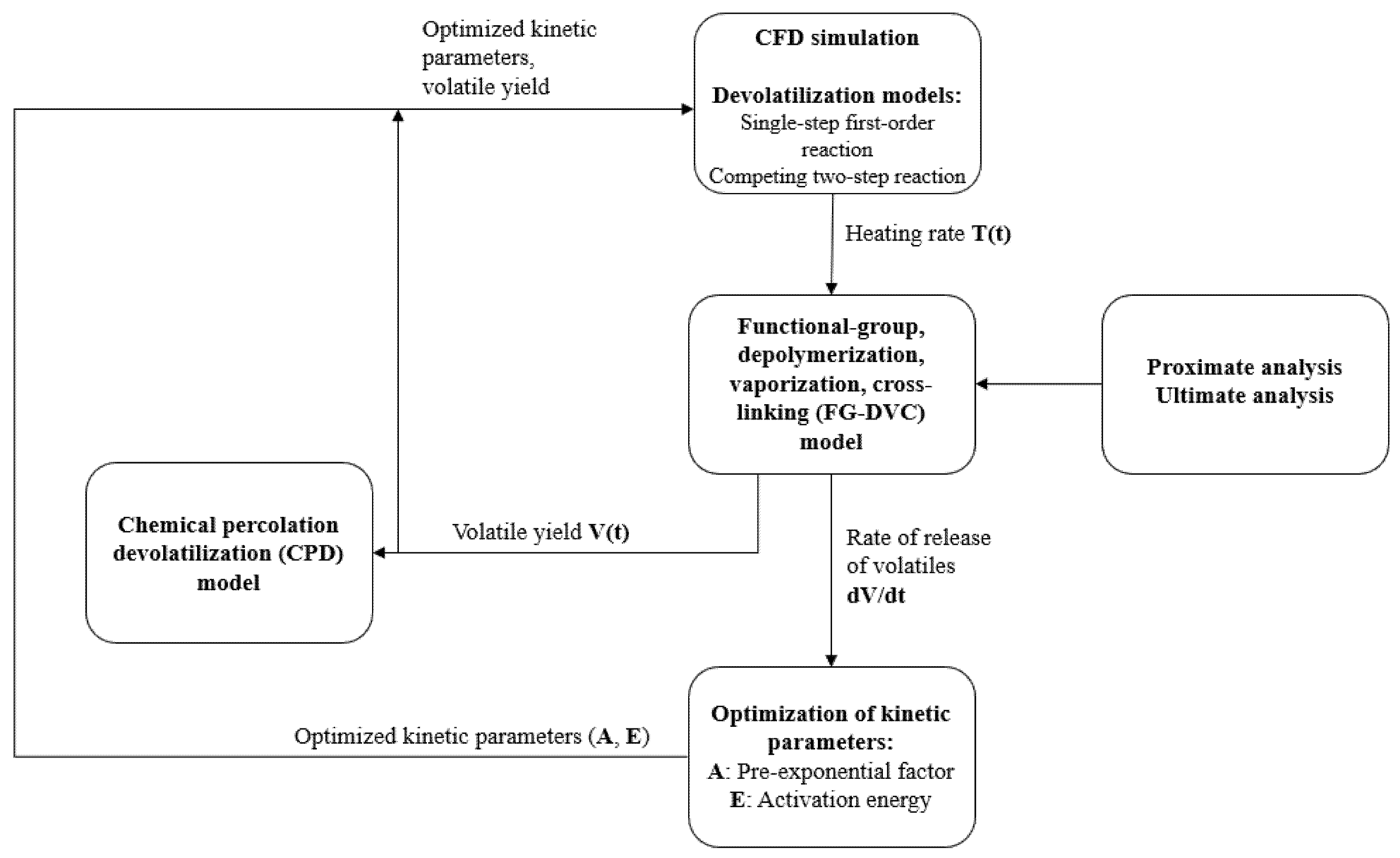
Devolatilization is modelled for each of the reactors according to the Mularski and Modliński optimization procedure [34]. The main benefit of this approach is that it considers the effect of operating conditions (heating rate and fuel properties) on the volatile matter release [35]. The optimization process (Figure 1) yields kinetic parameters (the activation energy and pre-exponential factor) for single-step first-order reaction model (SFOR) and competing two-step reaction model (C2SM), based on functional-group, depolymerization, vaporization, cross-linking model (FG-DVC) results, through the minimization of the objective function. FG-DVC is used independently of CFD, as a stand-alone model. Moreover, it estimates the volatile yield which is then incorporated into CFD. The reason why the three different devolatilization models are used (chemical percolation devolatilization model (CPD), SFOR, C2SM—Table 1) lies in the complexity of the particular reactors. The Mitsubishi Heavy Industries (MHI) reactor required the longest simulation time while the Brigham Young University (BYU) gasifier required the lowest computational cost. The global empirical models (SFOR, C2SM) allowed us to reduce the computational effort. It should be noted that the CFD-embedded CPD model used in the BYU reactor supplies only the volatiles release rate. Therefore, the final volatile yield for CPD is obtained using the FG-DVC approach. The input parameters for CPD are estimated applying the Genetti et al.’s correlation [36], which was found to provide satisfactory results in the literature considering combustion/gasification aspects [11,37,38,39].

The volatile matter evolved during devolatilization consists of tar, light gases, H₂O, CO, and CO₂. The tar molecule was assumed to be a C_xH_yO_z molecule with C₇ as the main component [40,41]. Light gases are treated as a C_mH_n molecule. It was also assumed that the volatiles are produced as a single compound which instantaneously breaks up into products. The final volatile composition has the following form:

$$\mathrm{Volatiles}\to {\mathrm{a}}_1{\mathrm{C}}_{\mathrm{x}}{\mathrm{H}}_{\mathrm{y}}{\mathrm{O}}_{\mathrm{z}}{+\mathrm{a}}_2{\mathrm{C}}_{\mathrm{m}}{\mathrm{H}}_{\mathrm{n}}{+\mathrm{a}}_3{\mathrm{CO}+\mathrm{a}}_4{\mathrm{H}}_2{\mathrm{O}+\mathrm{a}}_5{\mathrm{CO}}_2$$

(1)

where the ${\mathrm{a}}_{\mathrm{i}},\mathrm{x},\mathrm{y},\mathrm{z}$ coefficients are calculated from the FG-DVC results and the fundamental atom conservation equations. Description of the models and the applied parameters can be found in the Supplementary data.

3. Models for Reactive Flow Simulations of Chemical Reactions and Their Interaction with Turbulent Flow

The current study is based on the gas phase modelling approaches under conditions typical for the gasification process and its impact on the entrained flow reactor simulation results. In most practical real-life reactors, the flow is turbulent. Turbulence itself is currently not fully understood on the fundamental level. The turbulence–kinetics interaction needs to be modelled since the chemical source term is non-linear and cannot be easily calculated from Reynolds Averaged Navier–Stokes equation transported quantities.

As regards the non-premixed reactive turbulent flows, chemical reaction of the species, the local time-dependent mixing and heat transfer determine the processes that occur in the gas phase during the gasification process. The issue of key importance in the gas phase reaction modeling is the calculation of source terms in species transport equations. They are expressed as the average values of non-linear rates of a reaction. The simplest approach is to consider infinitely fast chemistry which stems from the observation that during high-temperature combustion most of the produced species rapidly reach chemical equilibrium. One can conclude that the mixing process of large eddies where the time scale is equal to k/ε controls the actual rate at which chemical reactions occur [42]. No kinetic information is required.

One of the most common infinitely fast assumption based models is the eddy dissipation model (EDM) [43]. The latest review of the CFD modeling of coal gasification [9] indicates that this approach is most widely used owing to its relatively simple form, robustness and numerical stability. Unfortunately, it lacks a direct interaction between turbulence and kinetics. This approach cannot accurately determine the reaction rates for multi-step reaction mechanisms and reversible reactions. The reason is that multi-step mechanisms are based on reaction rates occurring on various time scales, while in the eddy dissipation model every reaction has the same turbulent rate [42]. In the case of gasification the above mentioned assumptions might be oversimplified since there is an extended region with reacting flow with lower temperatures where chemical reaction rates are comparable to turbulent mixing rates. For example, CO oxidizes rapidly at high temperatures with oxygen presence, but does not oxidize so well at lower temperatures or less intensive mixing atmosphere. Such conditions are common in entrained flow gasifiers. Additionally, at high temperatures the dissociation reactions dominate. In such cases it is necessary to apply more detailed and complex approaches, which usually require the adoption of a finite-rate chemistry. The second approach used to model the influence of turbulence on chemical reactions is the eddy dissipation concept (EDC) [44]. EDC enables to account for detailed kinetics of reactions. In this model the total space is subdivided into the surrounding fluid and fine structures. Small-scale structures can be considered as a part of the control volume, where Kolmogorov-sized eddies containing combustion species are situated so closely, that mixing occurs on the molecular level [45]. Reactions of components that are reactive in nature are considered to take place only in such spaces which are locally treated as perfectly stirred (PSR) reactors, where the residence time is defined as

$${\mathsf{\tau }}^{\ast }=0.41\cdot \sqrt{\frac{\mathrm{v}}{\mathsf{ϵ}}}$$

(2)

where $\mathrm{v}$ is the kinematic viscosity, $\mathsf{ϵ}$ denotes turbulent kinetic energy dissipation rate. These parameters are calculated from turbulence model. Mass fraction occupied by fine structures is modeled as

$${\mathsf{\gamma }}^{\ast }={\left(2.13\cdot {\left(\frac{\mathrm{v}\mathsf{ϵ}}{{\mathrm{k}}^2}\right)}^{0.25}\right)}^2$$

(3)

The reaction rates of each species are calculated on a mass balance for the fine-structure reactor. Denoting quantities of fine structures with asterisk, the i species conservation equation can be expressed as follows [46]:

$$\frac{{\mathsf{\rho }}^{\ast }}{{\mathsf{\tau }}^{\ast }\left(1-{\mathsf{\gamma }}^{\ast }\right)}\left({\mathrm{m}}_{\mathrm{i}}^{\ast }-\overline{{\mathrm{m}}_{\mathrm{i}}}\right){=\mathrm{M}}_{\mathrm{i}}\cdot {\mathsf{\omega }}_{\mathrm{i}}^{\ast }$$

(4)

where $\overline{{\mathrm{m}}_{\mathrm{i}}}$ is the average mass fraction of the species i, ${\mathrm{M}}_{\mathrm{i}}$ is the molecular weight of the species i, ${\mathsf{\omega }}_{\mathrm{i}}^{\ast }$ is the chemical reaction rate calculated from Arrhenius equation. The mean net mass transfer rate of species i between the surrounding fluid and the fine structures can be described as

$${\mathrm{R}}_{\mathrm{i}}=\frac{{\overline{\mathrm{p}}\mathsf{\gamma }}^{\ast }}{{\mathsf{\tau }}^{\ast }\left({1-\mathsf{\gamma }}^{\ast }\right)}\left({\mathrm{m}}_{\mathrm{i}}^{\ast }-\overline{{\mathrm{m}}_{\mathrm{i}}}\right)$$

(5)

The EDC approach is applied in the CFD model and the non-linear system of equations in each control volume for the fine-structure reactor are solved which enables to determine the source term ${\mathrm{R}}_{\mathrm{i}}$ in transport equation of species i.

Modeling reactive flows that are turbulent in nature are computationally expensive. The cost increases with the number of chemical species involved in kinetic mechanism. The detailed kinetic mechanisms are adopted for combustion systems mostly with simple geometries and fuels that are characterized with the small number of species. For efficient computations the chemical kinetics mechanisms incorporated in the CFD simulations needs to be as small as possible. Devolatilization products of solid fuels consist of hydrocarbons for which a comprehensive mechanism is not available. For this reason, simplified kinetic reaction mechanisms were developed. The global mechanisms demonstrated in

Table 2. Examined global reaction mechanisms.

Reaction:	A (s-m-kmol)	Tb	Ea (J/kmol)
Mechanism 1
H2 + 0.5O2 → H2O	6.8 × 1015	0	1.67 × 108
CH4 + 0.5O2 → CO + 2H2	0.44 × 1012	0	1.2552 × 108
CH4 + H2O → CO + 3H2	0.30 × 109	0	1.2552 × 108
CO + H2O = CO2 + H2	0.275 × 1010	0	8.368 × 107
CO + 0.5O2 → CO2	2.24 × 1012	0	1.67 × 108
Mechanism 2
H2 + 0.5O2 → H2O	0.1 × 107	0	8.368 × 107
CH4 + 0.5O2 → CO + 2H2	0.44 × 1012	0	1.2552 × 108
CH4 + H2O → CO + 3H2	0.30 × 109	0	1.2552 × 108
CO + H2O = CO2 + H2	0.275 × 1010	0	8.368 × 107
Mechanism 3
H2 + 0.5O2 → H2O	1.00 × 107	0	8.368 × 106
CO + 0.5O2 → CO2	5.42 × 109	0	1.2552 × 108
CH4 + 1.5O2 → CO + 2H2O	7.28 × 109	0.5	1.67 × 108
Mechanism 4
CH4 + 0.5O2 → CO + 2H2	3.80 × 107	0	5.5463 × 107
CH4 + 1.5O2 → CO + 2H2O	2.33 × 1011	0.5	1.67 × 108
CO + 0.5O2 → CO2	1.30 × 1011	0	1.2552 × 108
Surface reactions for each Mechanism
C(s) + 0.5O2 → CO	5.09 × 108	0	1.79 × 104
C(s) + CO2 → 2CO	6.35 × 109	0	3.87 × 104
C(s) + H2O → CO + H2	1.90 × 107	0	3.51 × 104

are the most convenient and hence considered in this paper.

Mechanism 1 and Mechanism 2 are based on [47], but Mechanism 1 additionally incorporates the reaction of CO oxidation to CO₂ [48]. Mechanism 1 was often employed in gasification modeling. Mechanism 3 works under the assumption of a water–gas shift equilibrium. Mechanism 4 is mainly based on the one described in [49]. All of the examined approaches consider CH₄ to represent the reactions of hydrocarbons and tar

4. Ideal Plug Flow Reactor Study

Reduced mechanisms are mostly applied to decrease the computational effort. Their application is usually associated with accuracy loss, thus making the simulations unreliable. An effective solution is to compare global mechanisms with either experimental measurements or validated complex kinetic mechanisms. In the present paper the global hydrocarbon combustion mechanisms were compared with the detailed CRECK mechanism (1999 elementary chemical reactions, 115 species) [15,16] and with the detailed GRI-Mech 3.0 mechanism (325 elementary chemical reactions, 53 species) [14].

The objective of this section is to characterize the behavior of global reaction mechanisms under high-temperature gasification conditions. An investigation was carried out to indicate which global mechanism has the highest accuracy. The chosen detailed mechanisms were validated in various conditions. It must be mentioned that the validation range of GRI-Mech for pressure is up to 10 atm, whereas the validation range of CRECK is up to 100 atm. An additional comparison of these two approaches is made for pressures above 10 atm. This validation was necessary since GRI-Mech can be implemented into CFD model, while CRECK is simply too large to be used in 3-D reactive flow simulations due to computational effort.

The analysis provided almost identical results of GRI-Mech and CRECK for all examined conditions—Section 4. Owing to the fact that GRI-Mech is less computationally expensive, it will further serve as a reference data. As a result, we will assume that the global mechanism from Table 2 which results will be closest to GRI-Mech 3.0 brings the highest level of confidence.

The calculations have been performed with an in-house plug flow approach. GSL (GNU Scientific Library) libraries were used to solve the system of stiff differential equations. The main assumption of a plug flow reactor model is that the fluid is perfectly mixed in the direction perpendicular to the axis and that axial diffusive transport is negligible—Figure 2. Thus, the species continuity equation for the steady, constant cross-sectional plug flow is described as

$${\mathsf{\rho }\mathrm{u}}_{\mathrm{z}}\frac{{\mathrm{dY}}_{\mathrm{k}}}{\mathrm{dz}}{=\mathrm{R}}_{\mathrm{A}}$$

(6)

where $\mathsf{\rho }$ is density, ${\mathrm{u}}_{\mathrm{z}}$ is velocity in z direction, ${\mathrm{Y}}_{\mathrm{k}}$ is mass fraction of species k, $\mathrm{dz}$ is differential thickness of fluid plug, and ${\mathrm{R}}_{\mathrm{A}}$ is reaction rate.

Table 3. Input parameters for plug flow reactor (PFR).

Fuel Mixture, Mole Fraction	Oxidizer Mixture, Mole Fraction	Equivalence Ratio	Initial Gas Temperature
C(s)—0.677	H2O—0.22	2.2	800 K
CH4—0.284	N2—0.10
CO—0.039	O2—0.68

presents the input parameters for plug flow reactor (PFR).

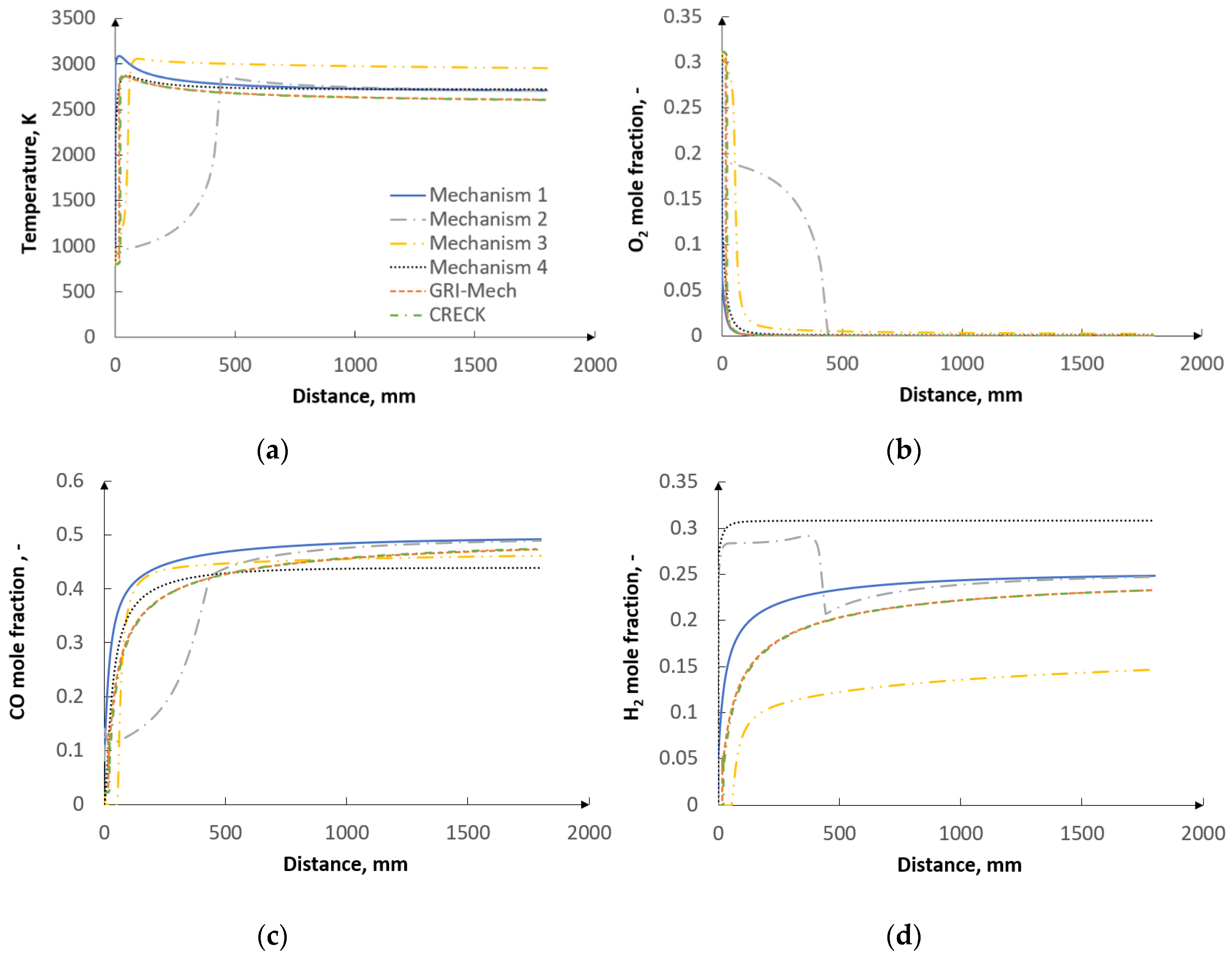
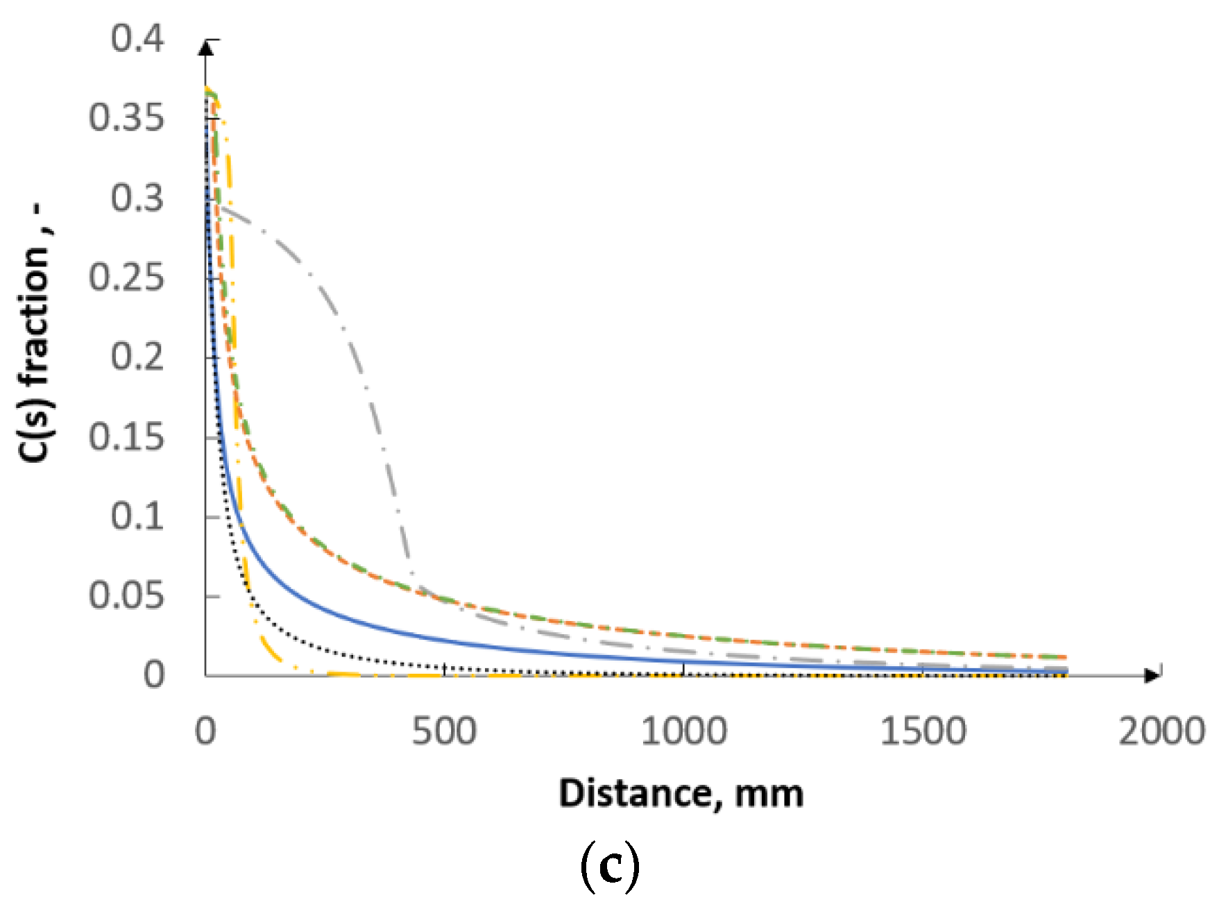
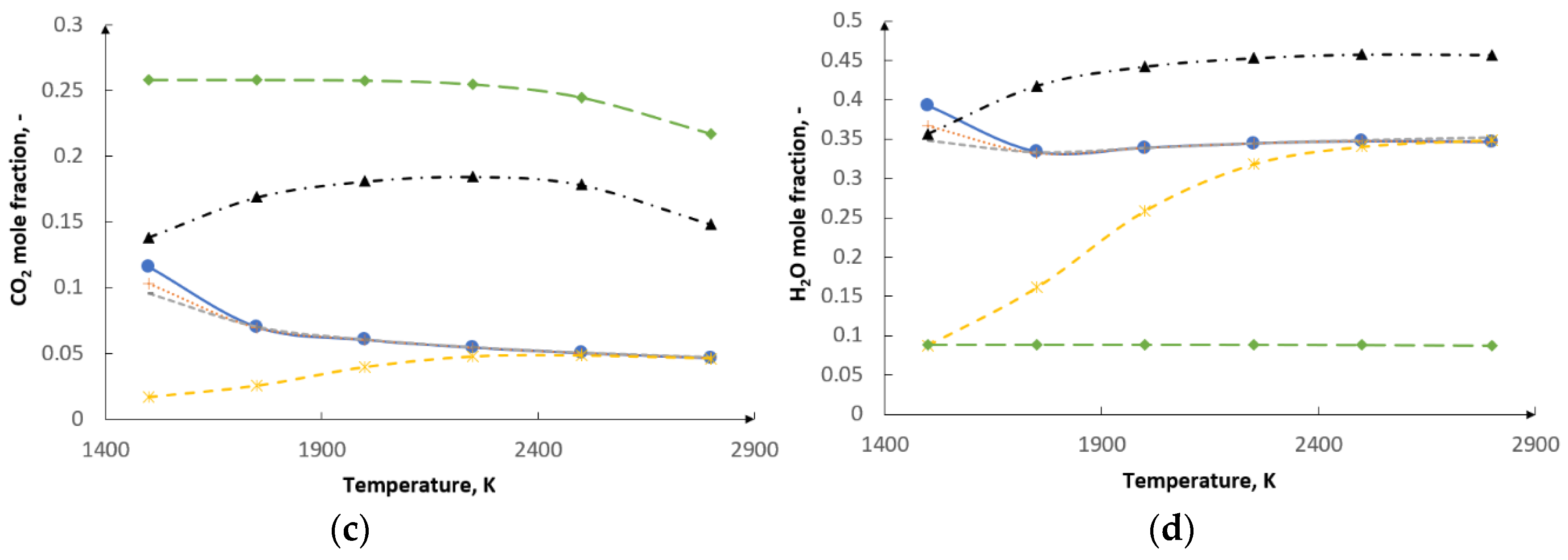
Figure 3a shows the temperature distribution in the PFR. One can notice that only Mechanisms 1 and 4 show close agreement with the GRI-Mech approach. Figure 3b–d show the O₂, CO, and H₂ mole fraction distributions. In this case, Mechanism 1 also reproduces the results with the highest accuracy with regard to GRI-Mech. Mechanism 2 exhibits the worst accuracy. As regards Figure 4, which depicts the CO₂, H₂O, and C(s) mole fraction distributions, Mechanism 1 also shows the best agreement with GRI-Mech, whereas Mechanism 2 reproduces the results with the worst accuracy. On the basis of these figures one can draw the conclusion that Mechanism 2 is the only examined mechanism which does not consider the oxidation reaction of CO ($\mathrm{CO}+{0.5\mathrm{O}}_2\to {\mathrm{CO}}_2$). The lack of this reaction substantially impacts the results. Moreover, for each distribution (Figure 3 and Figure 4) the results from Mechanisms 1 and 2 begin to converge after the distance of 500 mm. One can conclude that the impact of the CO oxidation reaction is most significant within the distance of 0–500 mm. With respect to GRI-Mech, Mechanisms 3 and 4 show poor agreement as well. It is evident that these approaches do not consider the water–gas shift reaction. The results from the CFD analysis (Section 7) confirm the great importance of this reaction in the accurate prediction of the gasification process. Therefore, one can ultimately conclude that, as regards the global reaction mechanisms, the $\mathrm{CO}+{0.5\mathrm{O}}_2\to {\mathrm{CO}}_2$ reaction and the ${\mathrm{CO}+\mathrm{H}}_2\mathrm{O}\to {\mathrm{CO}}_2{+\mathrm{H}}_2$ reaction have a substantial impact on the gas phase in gasification. Figure 4c shows the consumption of C(s) in the reactor. The strong impact of the gas phase reactions on the char consumption rate is apparent.

Judging by the overall accuracy, based on the error analysis, it is evident that Mechanism 1 shows the closest agreement with GRI-Mech and CRECK.

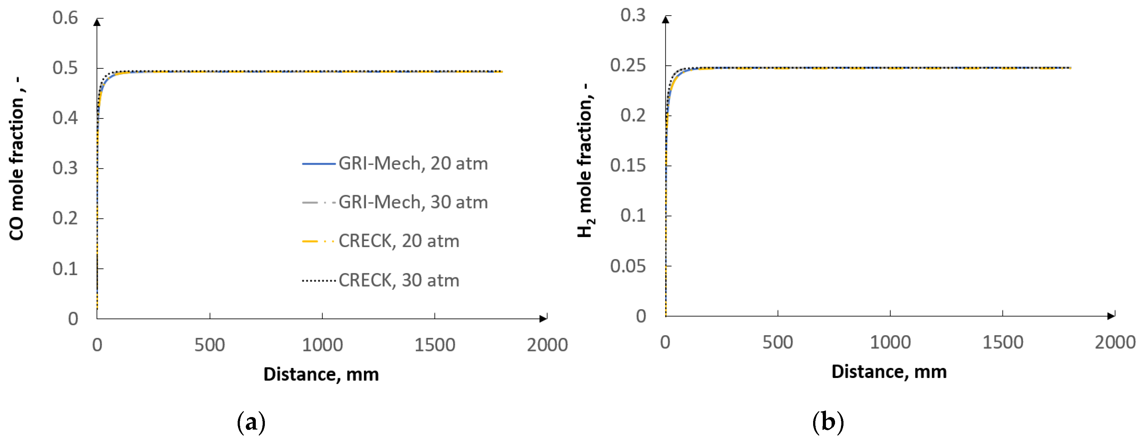
Figure 5 presents the exemplary results of GRI-Mech and CRECK for two pressures that are outside of the optimization range of GRI-Mech. An excellent agreement can be noticed proving that GRI-Mech can be surely utilized in high-pressure conditions. Section 5 analyzes the performance of global approaches in a perfectly stirred reactor study.

5. Ideal Perfectly Stirred Reactor Study

Perfectly stirred reactor study is the second part of ideal reactors study where global mechanisms from Table 2 are compared with detailed mechanisms in terms of the accuracy in temperature distribution or molar fraction distribution of the main syngas components.

The basic assumption of perfectly stirred reactor model is that the perfect mixing (homogeneity) is achieved inside the control volume—Figure 6.

Mass conservation for an arbitrary species i may be written as

$${\mathrm{R}}_{\mathrm{i}}{\mathrm{M}}_{\mathrm{i}}={\dot{\mathrm{m}}}_{\mathrm{i},\mathrm{out}}-{\dot{\mathrm{m}}}_{\mathrm{i},\mathrm{in}}$$

(7)

where ${\mathrm{R}}_{\mathrm{i}}$ is the net production rate of the ith species and ${\mathrm{M}}_{\mathrm{i}}$ is the molecular weight.

Table 4. Input parameters for perfectly stirred reactors (PSR).

Fuel Mixture, Mole Fraction	Oxidizer Mixture, Mole Fraction	Equivalence Ratio	Gas Temperatures	Pressure
C(s)—0.284	H2O—0.22	2.2	1500 K, 1750 K, 2000 K, 2250 K, 2500 K, 2800 K	20 atm
CH4—0.677	N2—0.10
CO—0.039	O2—0.68

presents the input parameters for PSR.

The analysis is conducted for six temperatures—1500 K, 1750 K, 2000 K, 2250 K, 2500 K, and 2800 K. Judging by Figure 7, one can notice an extremely close agreement of GRI-Mech, CRECK, and global Mechanism 1 for five out of six temperatures. For 1500 K there is a slight disagreement between these mechanisms. Mechanisms 3 and 4 depict the worst accuracy with respect to the detailed mechanisms. Mechanism 2 provides relatively close agreement for temperatures higher than 2000 K. Considering the plug flow reactor study and the perfectly stirred reactor study, in both examined cases Mechanism 1 exhibited the highest agreement with the detailed mechanisms. On this basis, Mechanism 1 will be further investigated as the main global approach in the CFD study. Based on the flow regime, plug flow reactor relates to the BYU gasifier, whereas perfectly stirred reactor relates to the MHI and E-gas gasifiers.

6. Reactors. Computational Domain

(a)

BYU reactor

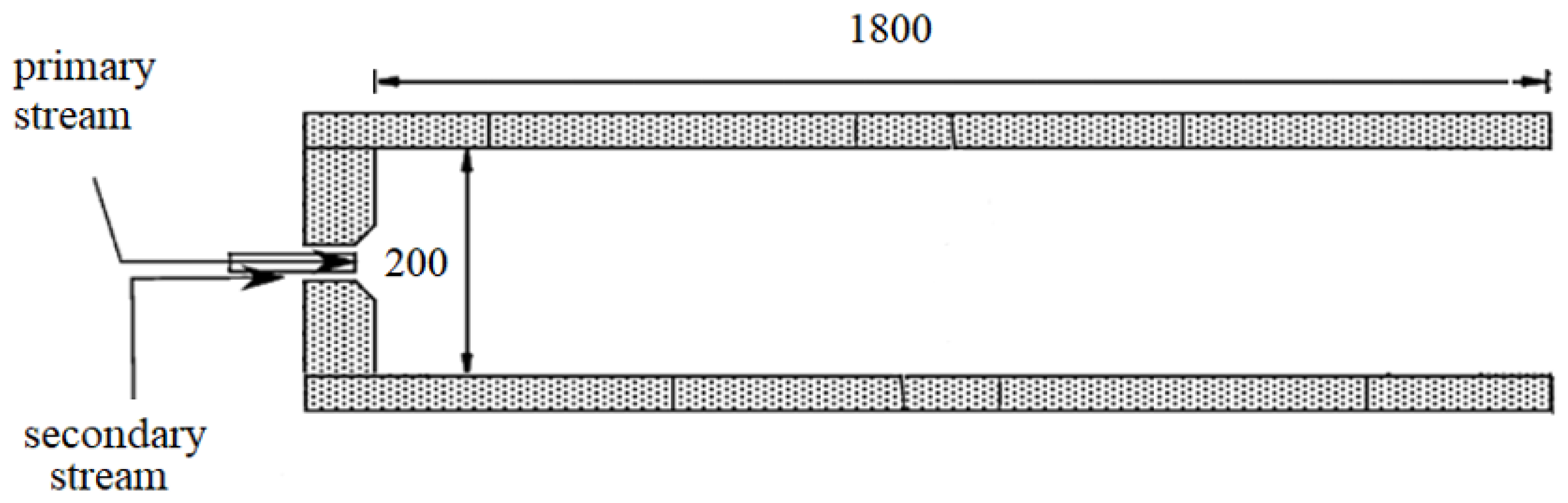
The BYU reactor is an oxygen-blown, one-stage entrained flow reactor with atmospheric pressure with a non-swirling flow (Figure 8). It has a diameter of 20 cm and is 1.8 m long. Bituminous pulverized coal from Utah was used in the investigations. The ultimate and proximate analysis are presented in

Table 5. Proximate and ultimate analyses of coals for three reactors.

Proximate Analysis, as Received
Utah Bit. Coal, % BYU Reactor		TH Coal, % MHI Reactor	Illinois Coal, % E-Gas Reactor
Volatile matter	45.6	46.8	35.0
Fixed carbon	43.7	35.8	44.2
Ash	8.3	12.1	9.7
Moisture	2.4	5.3	11.1
Ultimate analysis, % dry-ash-free
C	77.6	77.6	80.5
H	6.56	6.5	5.7
N	1.42	1.78	1.6
S	0.55	0.22	3.5

.

Coal was supplied in the primary stream with a gas consisting of O₂, Ar, and H₂O. The secondary stream contained only H₂O. The mass flow rates with molar fractions are presented in

Table 6. Mass flow rates of coal and gas with molar composition for BYU reactor.

1st Stage, kg/h	26.24
O2	0.85
Ar	0.126
H2O	0.024
2nd stage, kg/h	6.62
H2O	1
Utah bituminous coal, kg/h	23.88

. The particle size followed the Rosin–Rammler distribution.

$${\mathrm{Y}}_{\mathrm{d}}{=\mathrm{e}}^{-{\left(\frac{\mathrm{d}}{\overline{\mathrm{d}}}\right)}^{\mathrm{n}}}$$

(8)

The parameters applied in this study were as follows. The minimum, mean, and maximum diameters were equal to 1, 36, and 80 μm, respectively. The spread parameter was equal to 1.033. The kinetic parameters of the heterogeneous and homogeneous reactions were taken from the literature and are presented in

Table 7. Kinetic parameters for surface reactions and gas–phase reactions (global reaction approach).

Reactions:	Kinetic Parameters: A—kg/s Pa, E—J/kmol
	BYU Reactor	MHI Reactor	E-Gas Reactor
Surface reactions:
$\mathrm{C}\left(\mathrm{s}\right)+{0.5\mathrm{O}}_2\to \mathrm{CO}$	$\mathrm{A}=0.005$ $\mathrm{E}={7.4\times 10}^7$ [37]	$\mathrm{A}=0.052$ $\mathrm{E}={6.1\times 10}^7$ [51]	$\mathrm{A}=0.052$ $\mathrm{E}={6.1\times 10}^7$ [51]
$\mathrm{C}\left(\mathrm{s}\right){+\mathrm{CO}}_2\to 2\mathrm{CO}$	$\mathrm{A}=0.0635$ $\mathrm{E}={1.62\times 10}^8$ [37]	$\mathrm{A}=0.0732$ $\mathrm{E}={1.125\times 10}^8$ [51]	$\mathrm{A}=0.0732$ $\mathrm{E}={1.125\times 10}^8$ [51]
$\mathrm{C}\left(\mathrm{s}\right){+\mathrm{H}}_2\mathrm{O}\to {\mathrm{CO}+\mathrm{H}}_2$	$\mathrm{A}=0.0019$ $\mathrm{E}={1.47\times 10}^8$ [37]	$\mathrm{A}=0.0782$ $\mathrm{E}={1.15\times 10}^8$ [51]	$\mathrm{A}=0.0782$ $\mathrm{E}={1.15\times 10}^8$ [51]
Gas phase reactions:
${\mathrm{C}}_{\mathrm{x}}{\mathrm{H}}_{\mathrm{y}}{\mathrm{O}}_{\mathrm{z}}+\frac{\mathrm{x}-\mathrm{z}}{2}{\mathrm{O}}_2\to \mathrm{xCO}+\frac{\mathrm{y}}{2}{\mathrm{H}}_2$	$\mathrm{A}={4.4\times 10}^{11}$ $\mathrm{E}={1.25\times 10}^8$ [18]	$\mathrm{A}={4.4\times 10}^{11}$ $\mathrm{E}={1.25\times 10}^8$ [18]	$\mathrm{A}={4.4\times 10}^{11}$ $\mathrm{E}={1.25\times 10}^8$ [18]
${\mathrm{C}}_{\mathrm{x}}{\mathrm{H}}_{\mathrm{y}}{\mathrm{O}}_{\mathrm{z}}+\left(\mathrm{x}-\mathrm{z}\right){\mathrm{H}}_2\mathrm{O}\to \mathrm{xCO}+\left(\frac{\mathrm{y}}{2}+\mathrm{x}-\mathrm{z}\right){\mathrm{H}}_2$	${\mathrm{A}=3\times 10}^8$ $\mathrm{E}={1.25\times 10}^8$ [18]	${\mathrm{A}=3\times 10}^8$ $\mathrm{E}={1.25\times 10}^8$ [18]	${\mathrm{A}=3\times 10}^8$ $\mathrm{E}={1.25\times 10}^8$ [18]
${\mathrm{C}}_{\mathrm{m}}{\mathrm{H}}_{\mathrm{n}}+\frac{\mathrm{m}}{2}{\mathrm{O}}_2\to \mathrm{mCO}+\frac{\mathrm{n}}{2}{\mathrm{H}}_2$	$\mathrm{A}={4.4\times 10}^{11}$ $\mathrm{E}={1.25\times 10}^8$ [18]	$\mathrm{A}={4.4\times 10}^{11}$ $\mathrm{E}={1.25\times 10}^8$ [18]	$\mathrm{A}={4.4\times 10}^{11}$ $\mathrm{E}={1.25\times 10}^8$ [18]
${\mathrm{C}}_{\mathrm{m}}{\mathrm{H}}_{\mathrm{n}}{+\mathrm{H}}_2\mathrm{O}\to \mathrm{mCO}+\left(\frac{\mathrm{n}}{2}+1\right){\mathrm{H}}_2$	${\mathrm{A}=3\times 10}^8$ [18]	${\mathrm{A}=3\times 10}^8$ $\mathrm{E}={1.25\times 10}^8$ [18]	${\mathrm{A}=3\times 10}^8$ $\mathrm{E}={1.25\times 10}^8$ [18]
${\mathrm{CO}+\mathrm{H}}_2\mathrm{O}\to {\mathrm{CO}}_2{+\mathrm{H}}_2$	$\mathrm{A}=2.75$ [46] $\mathrm{E}={8.38\times 10}^7$ [47]	$\mathrm{A}={2.75\times 10}^9$ $\mathrm{E}={8.38\times 10}^7$ [47]	$\mathrm{A}=2.75$ [46] $\mathrm{E}={8.38\times 10}^7$ [47]
$\mathrm{CO}+{0.5\mathrm{O}}_2\to {\mathrm{CO}}_2$	$\mathrm{A}={2.24\times 10}^{12}$ $\mathrm{E}={1.67\times 10}^8$ [48]	$\mathrm{A}={2.24\times 10}^{12}$ $\mathrm{E}={1.67\times 10}^8$ [48]	$\mathrm{A}={2.24\times 10}^{12}$ $\mathrm{E}={1.67\times 10}^8$ [48]
${\mathrm{H}}_2+{0.5\mathrm{O}}_2\to {\mathrm{H}}_2\mathrm{O}$	$\mathrm{A}={6.8\times 10}^{15}$ $\mathrm{E}={1.67\times 10}^8$ [18]	$\mathrm{A}={6.8\times 10}^{15}$ $\mathrm{E}={1.67\times 10}^8$ [18]	$\mathrm{A}={6.8\times 10}^{15}$ $\mathrm{E}={1.67\times 10}^8$ [18]

. The reactors geometry was discretized applying a 2D axisymmetric grid consisting of approximately 100,000 rectangular cells. A grid independence study was carried out. The exemplary results are presented in the Supplementary data. The numerical simulation was validated against the experimental data of Smith et al. [17].

(b)

MHI reactor

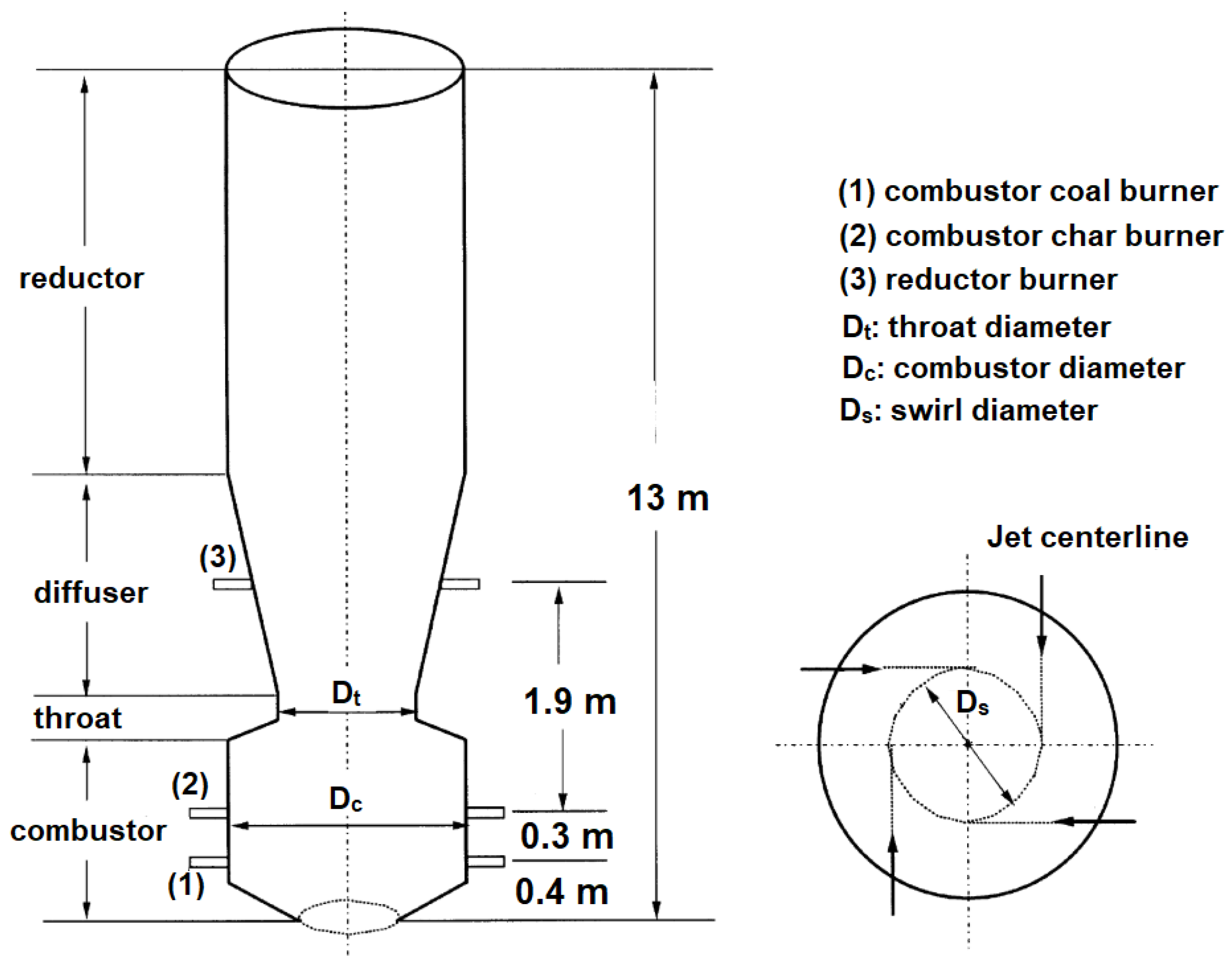
The MHI reactor is a 200 tons/day, two-stage, air-blown, and pressurized Mitsubishi entrained flow gasifier with a swirling flow (Figure 9). The reactor is 13 m long. It has three stages of dry-feed injectors. Two of them are located in the combustion region and the third one is in the reductor. Bituminous pulverized coal from Taiheiyo (TH) was used in the investigations. Its proximate and ultimate analyses are shown in Table 5.

Coal was injected with air in the 1st stage. Recycled char was injected through the second-stage injectors in the combustion region. The third-stage injectors were supplied with coal and air. The mass flow rates are presented in

Table 8. Mass flow rates of coal and gas for MHI reactor.

Mass Flow Rates of Coal in Three-Stage Injectors, kg/s
1st stage—coal	0.472
2nd stage—char	1.112
3rd stage—coal	1.832
Mass Flow Rates of Air, kg/s
1st stage	4.708
2nd stage	4.708
3rd stage	1.832

. The particle size followed the Rosin–Rammler distribution. The minimum, mean and maximum diameters were 4, 25, and 150 μm, respectively. The spread parameter was equal to 0.74. The kinetic parameters for the coal gasification reactions were taken from the literature—Table 7. The geometry of the reactor was discretized using a 3D planar grid consisting of approximately 530,000 elements. A grid independence study was carried out. The numerical model was validated against the experimental data of Chen et al. [51] and Watanabe et al. [52].

(c)

Conoco-Philips E-gas reactor

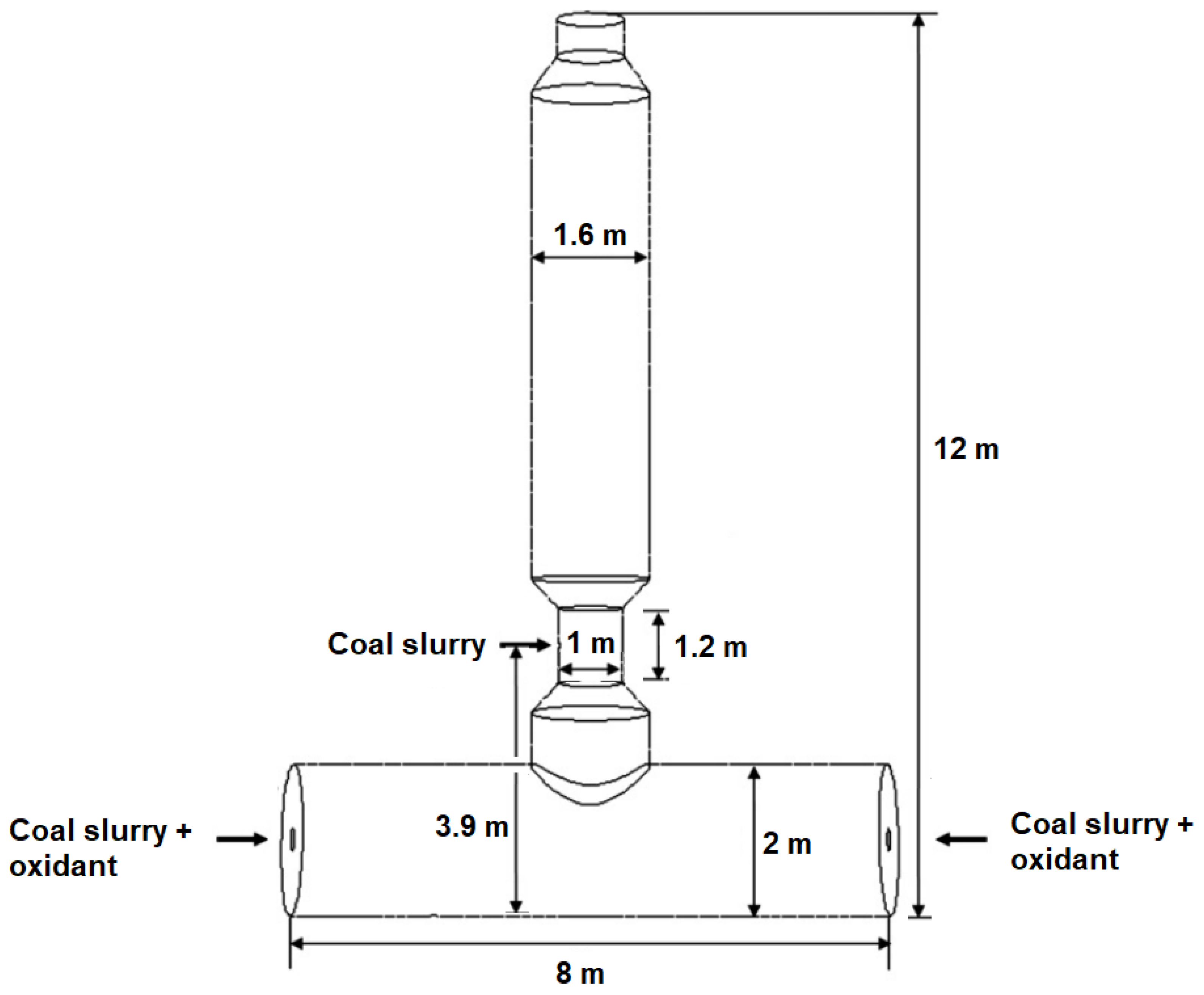
The Conoco-Philips E-gas reactor is a 2400 tons/day, two-stage, oxygen-blown, and pressurized entrained flow gasifier (Figure 10). It is 12 meters long. It has two stages of feed injectors. One of them is located in the combustor region and the second one in the throat. The combustor consists of an 8 m long horizontal cylinder with a diameter of 2 m. The first-stage injectors are located at each end of the combustor tube. Pulverized coal from Illinois was used in the investigations. Its proximate and ultimate analyses are shown in Table 5.

Coal–water slurry, oxygen and a small amount of nitrogen were injected in the first stage. In the second stage only coal–water slurry was injected. The mass flow rates are presented in

Table 9. Mass flow rates of coal and oxidant for E-gas reactor.

Mass Flow Rates of Coal in Three-Stage Injectors, kg/s
1st stage—coal	21.7
1st stage—water	9.3
2nd stage—coal	6.1
2nd stage—water	2.6
Mass Flow Rates of Oxidant, kg/s
1st stage (0.95 O2, 0.05 N2)	22.9
2nd stage	0

. The particle size was uniform and equal to 100 µm. The kinetic parameters are presented in Table 7. The geometry of the reactor was discretized using a 3D planar grid consisting of approximately 360,000 elements. A grid independence study was carried out. The numerical model was validated against the data of Shi et al. [19] and Labbafan et al. [53].

It was assumed that the reaction kinetics of C_xH_yO_z and C_mH_n with O₂ and H₂O were similar to those of light hydrocarbon molecules, such as CH₄ [18]. The choice is justified because these reaction rates do not vary greatly [47,48]. It is also apparent that the reaction kinetics of the gas phase is almost identical for the three examined reactors. The further discussion regarding the water–gas shift (WGS) reaction and its direct impact on the gasification process is presented in Section 7.4.

7. CFD Results

The results for each of the reactors are presented for the three cases:

• the global reaction approach with the finite-rate/eddy dissipation model (Global, laminar finite-rate/eddy dissipation model (F-R/EDM)),
• the global reaction approach with the eddy dissipation concept (Global, EDC),
• the detailed GRI-Mech mechanism with the eddy dissipation concept (GRI-Mech, EDC).

The global reaction approach is the extended Mechanism 1 (Section 4 and Section 5). The fourth case: the GRI-Mech mechanism with the finite-rate/eddy dissipation model (GRI-Mech, F-R/EDM) is not considered. GRI-Mech is a radical-reaction approach with reversible reactions which the finite-rate/eddy dissipation model cannot handle.

7.1. BYU Gasifier

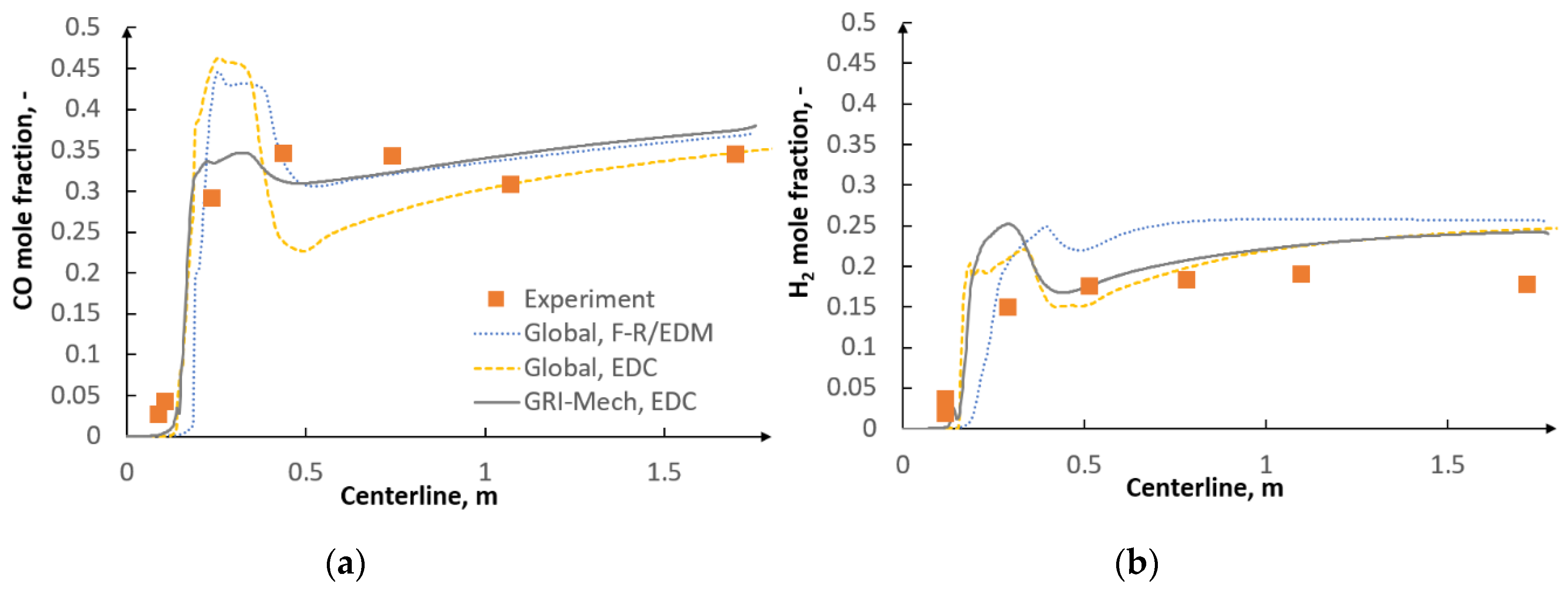
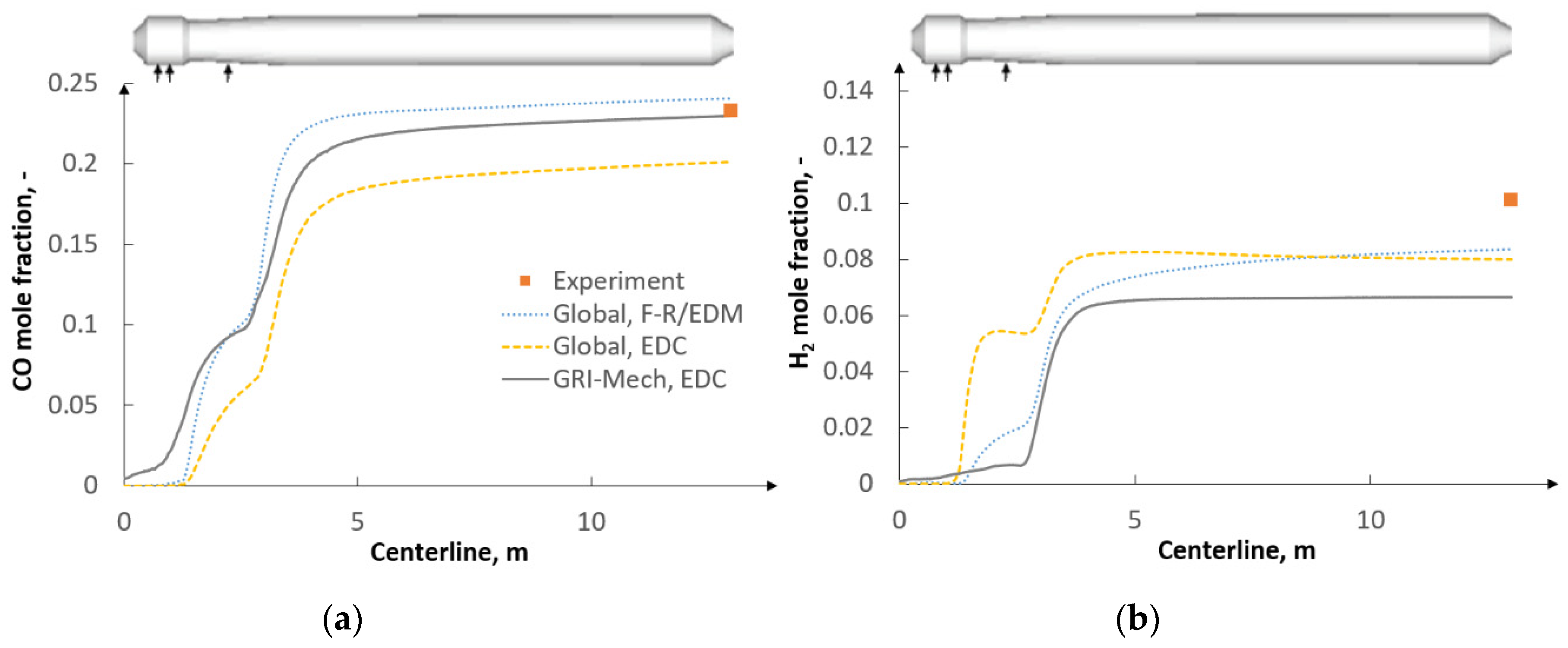
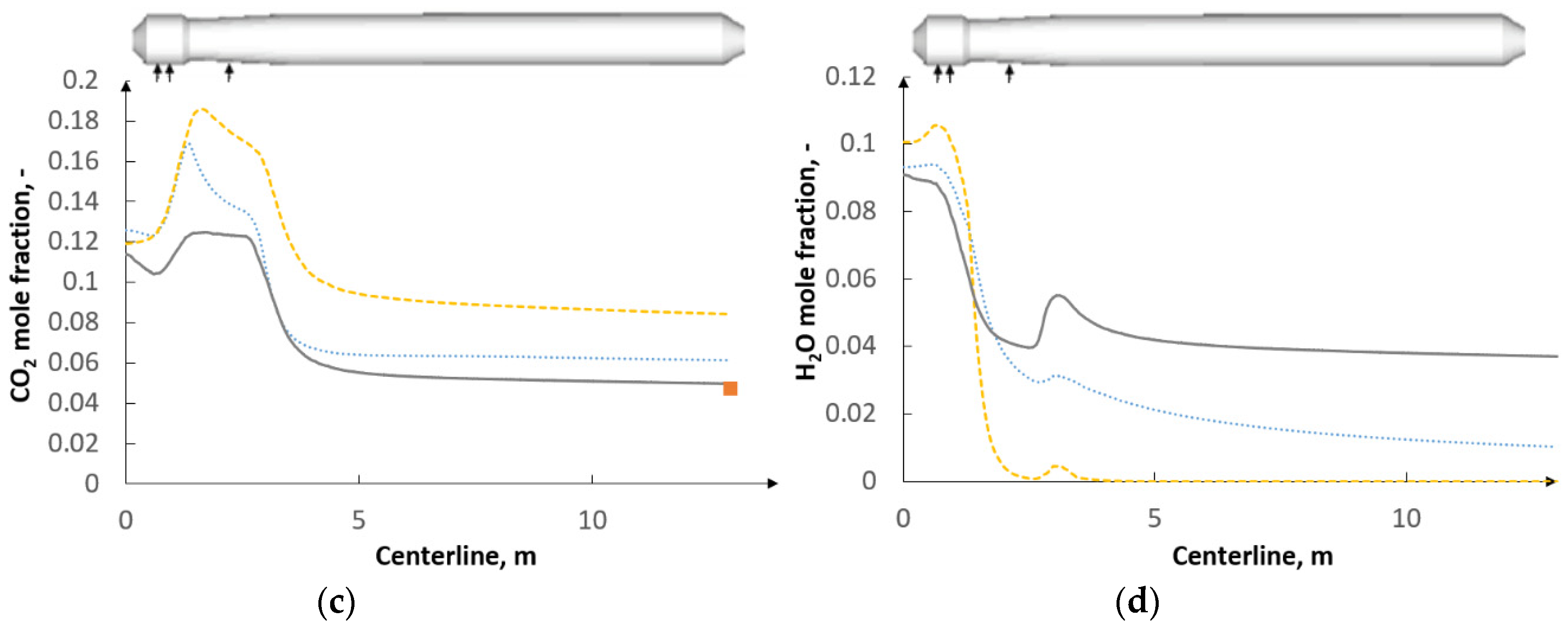
Figure 11 presents the molar fraction distribution of the main gas components (CO, H₂, CO₂ and H₂O) along the centerline inside the reactor. A strong impact of the examined gas phase modeling approaches on the gas composition inside the reactor, especially in the flame region, is visible. (Global, EDC) and (GRI-Mech, EDC) show closer agreement with each other than (Global, F-R/EDM) with (Global, EDC). This indicates that the turbulence–chemistry interaction has a greater impact on the gas composition than the reaction mechanisms. Considering the accuracy of the analyzed approaches, the GRI-Mech mechanism with the eddy dissipation concept yields the most accurate results with regard to the experimental data. (Global, F-R/EDM) predicts a strong peak in the CO yield in the flame region. On the other hand, the CO₂ and H₂O yields in the flame region estimated by (Global, F-R/EDM) are strongly underpredicted.

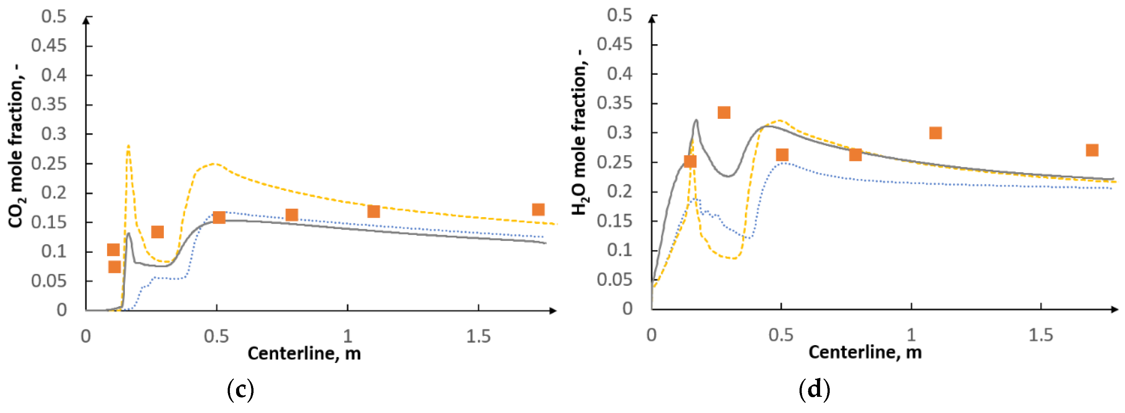
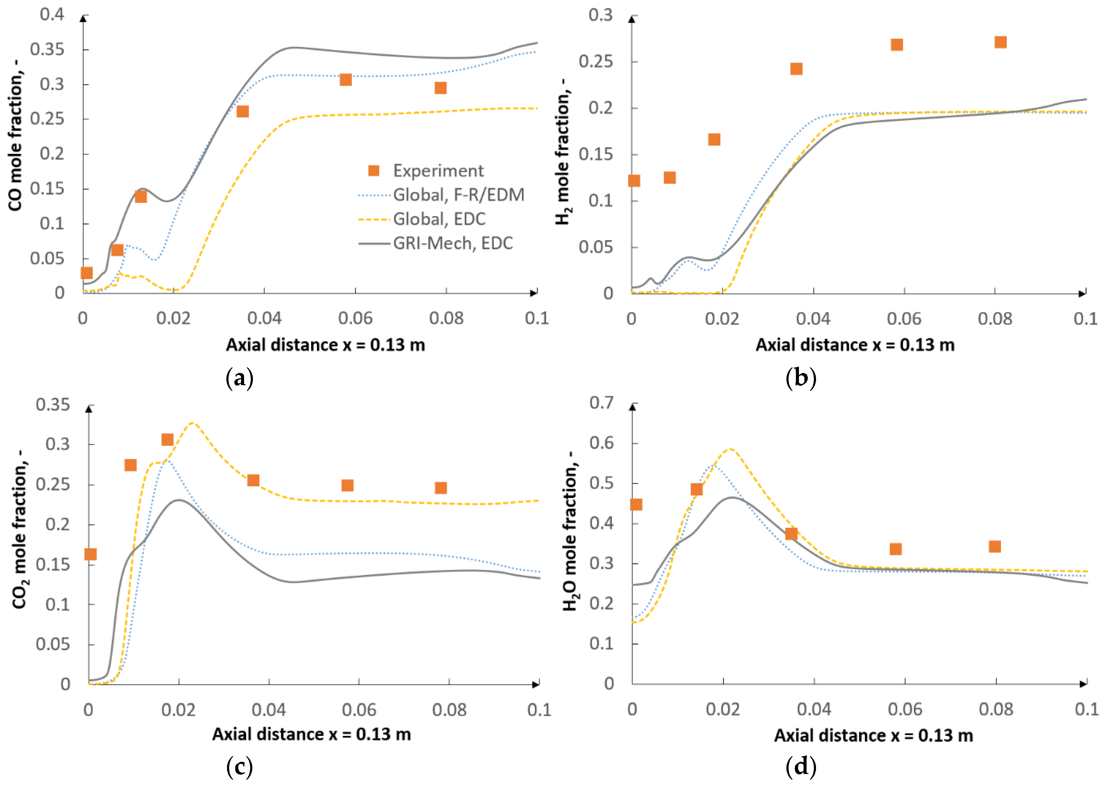
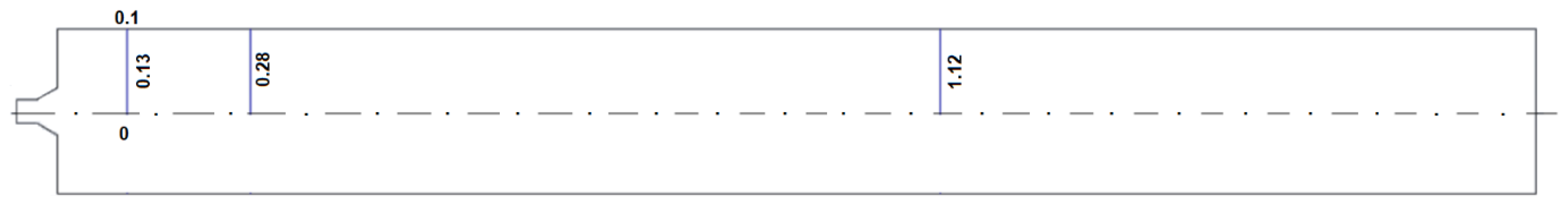
Figure 12, Figure 13 and Figure 14 depict the gas concentration for the radial traverses x = 0.13 m, x = 0.28 m and x = 1.12 m, respectively. The traverses are shown in Figure 15. The value of 0 in Figure 12, Figure 13 and Figure 14 in the horizontal ordinate indicates that the concentration is measured along the centerline. The value of 0.1 means that the concentration is measured close to the reactor wall.

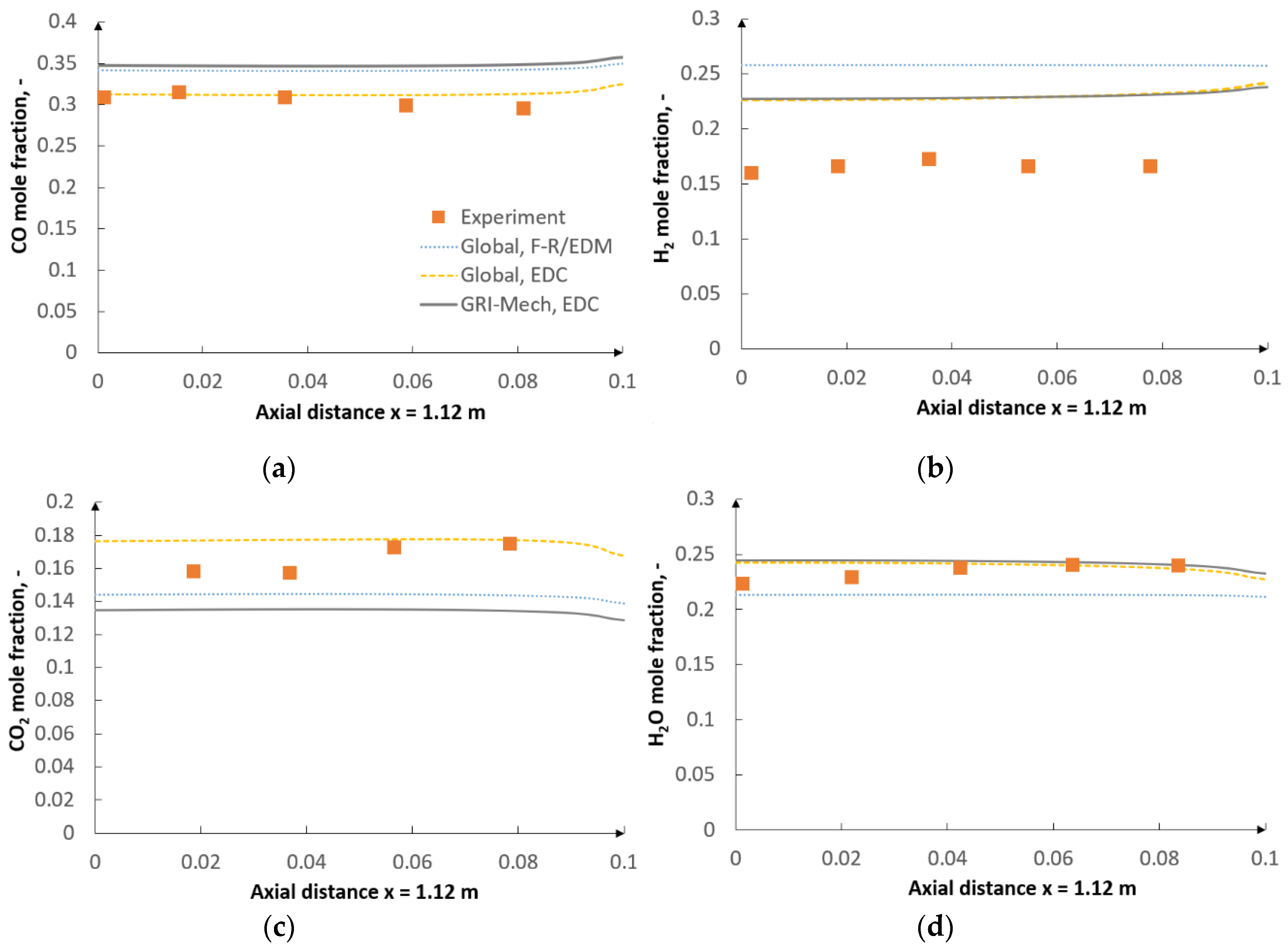
The models show great variations, especially for x = 0.13 m and x = 0.28 m in the flame region. (Global, EDC) and (GRI-Mech, EDC) yielded more accurate results than (Global, F-R/EDM). The recirculation zone was relatively well predicted, especially for CO and CO₂.

7.2. MHI Gasifier

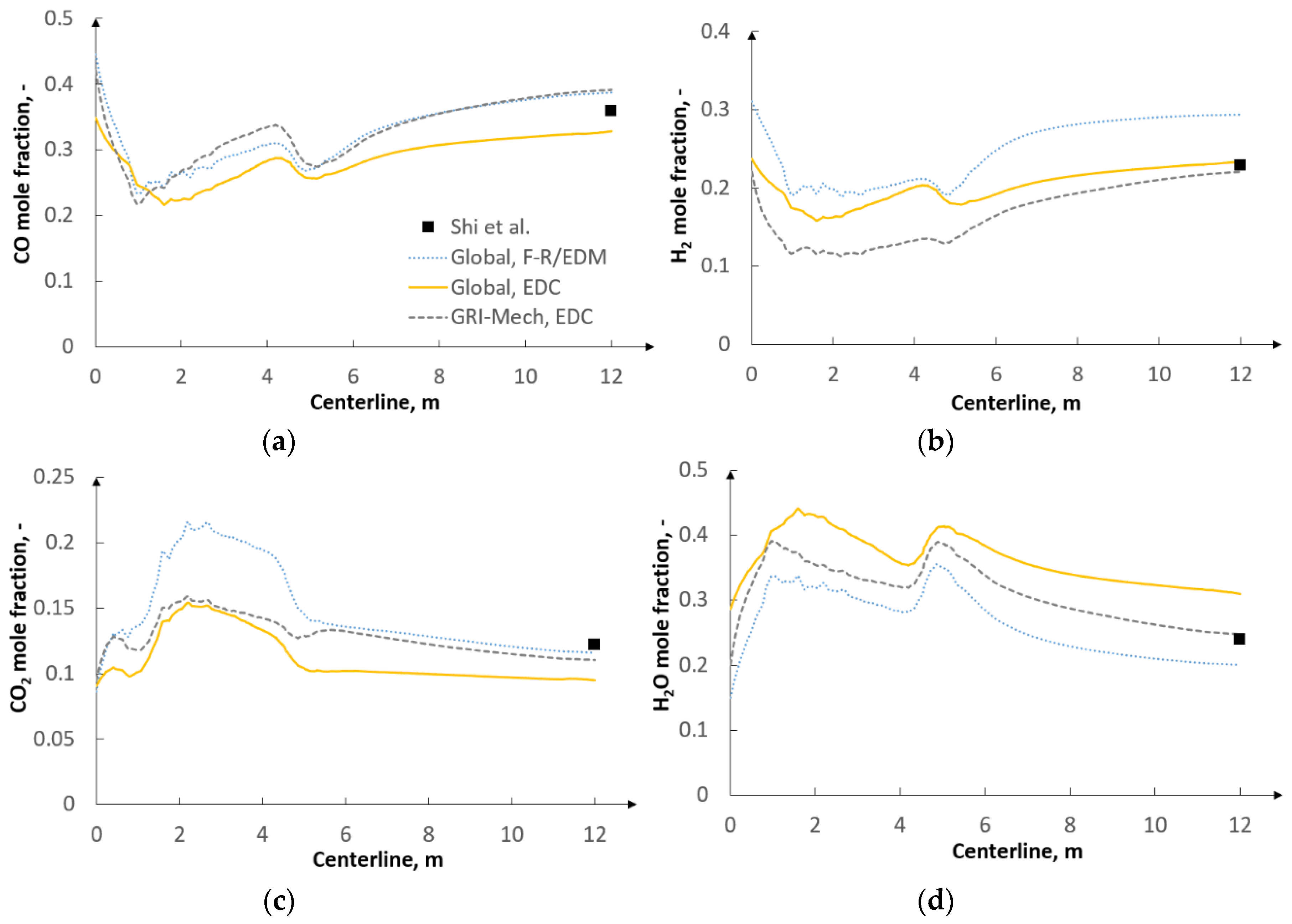
Figure 16 shows the mole fraction distribution of the main gas components in the MHI reactor. One can see a considerable increase in CO and H₂ concentration in the second stage of the reactor where endothermic gasification reactions prevail. On the other hand, the CO₂ and H₂O content gradually decreases as CO₂ and H₂O react with char to form CO and H₂. The GRI-Mech mechanism with the eddy dissipation concept turned out to be the most accurate approach when estimating CO and CO₂ concentration with respect to the outlet experimental data. However, the H₂ concentration was underpredicted by GRI-Mech. Its concentration was properly reproduced by the (Global, EDC) approach.

As regards H₂O concentration, no outlet experimental data points were available. (GRI-Mech, EDC) predicts H₂O molar concentration at the reactor outlet to be at 4–5%. (Global, F-R/EDM) and (Global, EDC) do not predict any amount of H₂O. This effect was attributed to the kinetics of the water–gas shift (WGS) reaction. In the case of the MHI gasifier, a very high reaction rate had to be assumed for the global reaction approach in order to match the experimental data (Table 9). This results in the consumption of all the H₂O. GRI-Mech, on the other hand, does not incorporate this reaction directly because the gas phase is modelled via radical reactions. Figure 16 also shows, as in the case of the BYU reactor, a relatively strong impact of the applied gas phase modeling approaches on gas composition. Both the eddy dissipation concept and the finite-rate/eddy dissipation model yield similar results for CO and H₂O concentrations along the centerline. In the case of CO₂ concentration, a substantial difference can be observed in the combustor region, where the eddy dissipation concept predicts a much higher concentration. Unfortunately, no experimental measurements in the combustor were available to confront the data. The most significant difference was noticed for H₂ concentration.

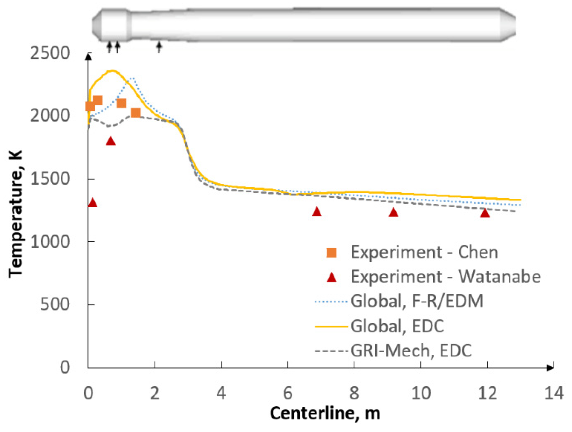
Figure 17 shows the temperature distribution along the centerline of the reactor. One can notice a substantial difference between the examined approaches in the combustor region. GRI-Mech yielded the most accurate results, predicting also lower temperatures than the global reaction approaches. A lower temperature predicted by GRI-Mech, in comparison with the other numerical approaches, indicates a lower CO₂ concentration in the combustor (Figure 16).

7.3. E-Gas Gasifier

Figure 18 shows the gas composition along the centerline for the E-gas reactor. As in the MHI reactor, an increase in CO and H₂ gas content can be noticed in the second stage of the E-gas reactor due to gasification reactions with CO₂ and H₂O. As a result, the CO₂ and H₂O content in the second stage gradually decreases. The CO₂ content is the highest in the combustor due to the relatively high O₂ concentration where the complete oxidation of C(s) with O₂ occurs. GRI-Mech with EDC is found to yield the most accurate results with regard to the outlet data obtained in [19]. The global reaction approach with the finite-rate/eddy dissipation model reproduces the results with the worst accuracy. Figure 19 shows the temperature distribution along the centerline of the reactor. One can notice that the GRI-Mech mechanism predicts lower temperatures in the combustor. The same is observed for the MHI reactor. The results confirm a substantial influence of the gas phase modeling approaches on gas composition and temperature distribution.

7.4. Water–Gas Shift Reaction

As regards the global reaction approach, the water–gas shift (WGS) reaction was observed to have a significant influence on the final gas composition. According to the literature review [52,54,55,56,57,58,59,60,61], the kinetic parameters for this reaction originate from the Jones–Lindstedt approach [47]. However, some authors modified the pre-exponential factor from this reaction [18,56,62,63,64] in order to match the experimental data. The reason lies in the fact that the rate from the Jones–Lindstedt mechanism was obtained under catalytic conditions which, in many cases, turned out to be too fast for gasification. The present study analyzes the behavior of the WGS reaction in three different gasification conditions. For the BYU gasifier, where the maximum flame temperature reached 2800 K, the kinetic parameters had to be very low to match the experimental data. The pre-exponential factor was assumed to be equal to 2.75. This value was taken from the study of Lu and Wang [62]. As regards the MHI reactor, where the maximum flame temperature was below 2400 K, the pre-exponential factor was assumed to be equal to 2.75 × 10⁹ and was taken from [63]. In the case of the E-gas gasifier, the flame temperature was observed to be above 3000 K and the pre-exponential factor was also assumed to be equal to 2.75 (

Table 10. Kinetic parameters of water–gas shift (WGS) reaction.

Reactor	MHI	BYU	E-Gas
Oxidant	air	O2	O2
Maximum flame temperature	$<2400 \mathrm{K}$	$<2800 \mathrm{K}$	$>3000 \mathrm{K}$
Kinetic parameters of WGS reaction A—kg/s Pa, E—kJ/mol	$\mathrm{A}={2.75\times 10}^9$ $\mathrm{E}=83.8$	$\mathrm{A}=2.75$ $\mathrm{E}=83.8$	$\mathrm{A}=2.75$ $\mathrm{E}=83.88$

). This observation confirms a very important feature of the WGS reaction, i.e., decreasing conversion with increasing temperature. However, such a wide range of pre-exponential factors (from 2.75 to 2.75 × 10⁹) makes it necessary to properly optimize this reaction rate prior to any numerical simulation.

Figure 20 shows the final gas composition for the (Global, F-R/EDM) approach at the BYU and E-gas reactor outlets for two pre-exponential factors (A = 2.75 and A = 2.75 × 10⁹) of the WGS reaction. One can notice a substantial difference in the gas composition at the reactor outlet, which confirms a strong dependence of this reaction on the operating conditions inside the gasifier. The pre-exponential factor value used for the MHI reactor (A = 2.75 × 10⁹) failed to correctly reproduce the outlet results for the BYU and E-gas gasifiers. The necessity of the proper optimization of the WGS rate can be overcome by directly implementing the GRI-Mech mechanism which was found to be the most accurate approach for each of the reactors. This is because GRI-Mech does not directly account for the WGS reaction as it is a radical–reaction approach.

8. Conclusions

In this paper a plug flow reactor study, a perfectly stirred reactor study and a CFD analysis were carried out to investigate the impact of chemical reaction mechanisms and turbulence–chemistry interaction approaches on coal gasification in entrained flow reactors with the aim of understanding which mechanisms are more accurate and suitable for gasification. The conclusions are as follows:

• Among the studied global reaction mechanisms in ideal PFR and PSR reactors, Mechanism 1 exhibited the highest agreement with regard to the detailed GRI-Mech and CRECK mechanisms.
• An excellent agreement between the detailed GRI-Mech and CRECK mechanisms could be noticed in the PFR and PSR reactors. Additionally, GRI-Mech was found to yield accurate results for pressure conditions outside of its validation range based on the comparison with CRECK.
• As regards the CFD study, the examined reaction mechanisms and turbulence–chemistry interaction approaches were found to have a significant impact on gas composition and temperature distribution inside the studied gasifiers.
• The detailed GRI-Mech mechanism with the eddy dissipation concept yielded the most accurate results with regard to the experimental data. The global reaction approach with the finite-rate/eddy dissipation model reproduced the results with the worst accuracy, even though it was found to be the approach most widely used in the literature.
• GRI-Mech was found to predict lower temperatures and especially CO₂ and H₂ concentrations in the flame region than the global reaction mechanism.
• Higher disagreement between the detailed and the global reaction mechanism approach was more remarkable in the CFD study than in the ideal reactor studies (PFR and PSR).
• From among the gas phase reactions, the water–gas shift (WGS) reaction and the CO oxidation reaction were found to significantly depend on the operating conditions inside the reactors.

References

- Zaini, I.N.; Gomez-Rueda, Y.; García López, C.; Ratnasari, D.K.; Helsen, L.; Pretz, T.; Jönsson, P.G.; Yang, W. Production of H2-rich syngas from excavated landfill waste through steam co-gasification with biochar. Energy 2020, 207, 118208. [Google Scholar] [CrossRef]
- Held, J. Gasification–Status and Technology; Rapport SGC 240; Swedish Gas Technology Centre: Malmö, Sweden, 2012; pp. 1–48. [Google Scholar]
- Li, J.; Paul, M.C.; Younger, P.L.; Watson, I.; Hossain, M.; Welch, S. Combustion Modelling of Pulverized Biomass Particles at High Temperatures. Phys. Procedia 2015, 66, 273–276. [Google Scholar] [CrossRef] [Green Version]
- Klimanek, A.; Adamczyk, W.; Katelbach-Woźniak, A.; Węcel, G.; Szlęk, A. Towards a hybrid Eulerian-Lagrangian CFD modeling of coal gasification in a circulating fluidized bed reactor. Fuel 2015, 152, 131–137. [Google Scholar] [CrossRef]
- Drikakis, D.; Frank, M.; Tabor, G. Multiscale computational fluid dynamics. Energies 2019, 12, 3272. [Google Scholar] [CrossRef] [Green Version]
- Shamooni, A.; Cuoci, A.; Faravelli, T.; Sadiki, A. Prediction of combustion and heat release rates in non-premixed syngas jet flames using finite-rate scale similarity based combustion models. Energies 2018, 11, 2464. [Google Scholar] [CrossRef] [Green Version]
- Della Torre, A.; Montenegro, G.; Onorati, A.; Khadilkar, S.; Icarelli, R. Multi-Scale CFD Modeling of Plate Heat Exchangers Including Offset-Strip Fins and Dimple-Type Turbulators for Automotive Applications. Energies 2019, 12, 2965. [Google Scholar] [CrossRef] [Green Version]
- Mahmoud, R.; Jangi, M.; Fiorina, B.; Pfitzner, M.; Sadiki, A. Numerical investigation of an oxyfuelnon-premixed combustion using a hybrid eulerian stochastic field/flamelet progress variable approach: Effects of H2/CO2 Enrichment and Reynolds Number. Energies 2018, 11, 3158. [Google Scholar] [CrossRef] [Green Version]
- Mularski, J.; Pawlak-Kruczek, H.; Modlinski, N. A review of recent studies of the CFD modelling of coal gasification in entrained flow gasifiers, covering devolatilization, gas-phase reactions, surface reactions, models and kinetics. Fuel 2020, 271, 1–36. [Google Scholar] [CrossRef]
- Park, S.S.; Jeong, H.J.; Hwang, J. 3-D CFD modeling for parametric study in a 300-MWe one-stage oxygen-blown entrained-bed coal gasifier. Energies 2015, 8, 4216–4236. [Google Scholar] [CrossRef] [Green Version]
- Vascellari, M.; Cau, G. Influence of turbulence-chemical interaction on CFD pulverized coal MILD combustion modeling. Fuel 2012, 101, 90–101. [Google Scholar] [CrossRef]
- Modlinski, N.; Hardy, T. Development of high-temperature corrosion risk monitoring system in pulverized coal boilers based on reducing conditions identification and CFD simulations. Appl. Energy 2017, 204, 1124–1137. [Google Scholar] [CrossRef]
- Wang, L.; Liu, Z.; Chen, S.; Zheng, C. Comparison of different global combustion mechanisms under hot and diluted oxidation conditions. Combust. Sci. Technol. 2012, 184, 259–276. [Google Scholar] [CrossRef]
- Smith, G.; Golden, D.; Frenklach, M.; Moriarty, N.; Eiteneer, B.; Goldenberg, M.; Bowman, C.; Hanson, R.; Song, S.; Gardiner, W.; et al. GRI-Mech 3. Available online: http://combustion.berkeley.edu/gri-mech/version30/text30.html (accessed on 14 October 2018).
- Ranzi, E.; Cavallotti, C.; Cuoci, A.; Frassoldati, A.; Pelucchi, M.; Faravelli, T. New reaction classes in the kinetic modeling of low temperature oxidation of n-alkanes. Combust. Flame 2015, 162, 1679–1691. [Google Scholar] [CrossRef]
- Ranzi, E.; Frassoldati, A.; Stagni, A.; Pelucchi, M.; Cuoci, A.; Faravelli, T. CRECK Modeling. Available online: http://creckmodeling.chem.polimi.it/menu-kinetics/menu-kinetics-detailed-mechanisms/107-category-kinetic-mechanisms/399-mechanisms-1911-c1-c3-ht (accessed on 28 November 2020).
- Brown, B.W.; Smoot, L.D.; Smith, P.J.; Hedman, P.O. Measurement and prediction of entrained-flow gasification processes. AIChE J. 1988, 34, 435–446. [Google Scholar] [CrossRef]
- Kumar, M.; Ghoniem, A.F. Multiphysics Simulations of Entrained Flow Gasification. Part II;: Constructing and Validating the Overall Model. Energy Fuels 2012, 26, 464–479. [Google Scholar] [CrossRef]
- Shi, S.-P.; Zitney, S.E.; Shahnam, M.; Syamlal, M.; Rogers, W.A. Modelling coal gasification with CFD and discrete phase method. J. Energy Inst. 2006, 79, 217–221. [Google Scholar] [CrossRef]
- Ansys Fluent User Guide. Available online:https://www.sharcnet.ca/Software/Ansys/18.2.2/en-us/help/ai_sinfo/flu_intro.html (accessed on 9 March 2019).
- Patankar, S.; Spalding, D. A calculation procedure for heat, mass and momentum transfer in three-dimensional parabolic flows. Int. J. Heat Mass Transf. 1972, 15, 1787–1806. [Google Scholar] [CrossRef]
- Crowe, C.; Sharma, M.P.; Stosk, D.E. The Particle-source-in Cell (PSI-CELL) Model for Gas-droplet Flows. J. Fluids Eng. 1977, 99, 325–332. [Google Scholar] [CrossRef]
- Shih, T.-H.; Liou, W.W.; Shabbir, A.; Yang, Z.; Zhu, J. A new k-ϵ eddy viscosity model for high reynolds number turbulent flows. Comput. Fluids 1995, 24, 227–238. [Google Scholar] [CrossRef]
- Dukowicz, J.K. A particle-fluid numerical model for liquid sprays. J. Comput. Phys. 1980, 35, 229–253. [Google Scholar] [CrossRef]
- Smith, I.W. The combustion rates of coal chars: A review. Symp. Combust. 1982, 19, 1045–1065. [Google Scholar] [CrossRef]
- Grant, D.M.; Pugmire, R.J.; Fletcher, T.H.; Kerstein, A.R. Chemical Model of Coal Devolatilization Using Percolation Lattice Statistics. Energy Fuels 1989, 3, 175–186. [Google Scholar] [CrossRef]
- Fletcher, T.H.; Kerstein, A.R.; Pugmire, R.J.; Grant, D.M. Chemical percolation model for devolatilization. 2. Temperature and heating rate effects on product yields. Energy Fuels 1990, 4, 54–60. [Google Scholar] [CrossRef]
- Scott, S.A.; Dennis, J.S.; Davidson, J.F.; Hayhurst, A.N. An algorithm for determining the kinetics of devolatilisation of complex solid fuels from thermogravimetric experiments. Chem. Eng. Sci. 2006, 61, 2339–2348. [Google Scholar] [CrossRef]
- Solomon, P.R.; Hamblen, D.G.; Carangelo, R.M.; Serio, M.A.; Deshpande, G.V. General Model of Coal Devolatilization. ACS Div. Fuel Chem. Prepr. 1987, 32, 83–98. [Google Scholar] [CrossRef]
- Badzioch, S.; Hawksley, P. Kinetics of thermal decomposition of pulverized coal particles. Ind. Eng. Chem. Process Des. Dev. 1970, 9, 521–530. [Google Scholar] [CrossRef]
- Anthony, D.B.; Howard, J.B.; Hottel, H.C.; Meissner, H.P. Rapid devolatilization of pulverized coal. Symp. Combust. 1975, 15, 1303–1317. [Google Scholar] [CrossRef]
- Kobayashi, H.; Howard, J.B.; Sarofim, A.F. Coal devolatilization at high temperatures. Symp. Combust. 1977, 16, 411–425. [Google Scholar] [CrossRef]
- Solomon, P.R.; Colket, M.B. Coal devolatilization. Symp. Combust. 1979, 17, 131–143. [Google Scholar] [CrossRef]
- Mularski, J.; Modliński, N. Entrained flow coal gasification process simulation with the emphasis on empirical devolatilization models optimization procedure. Appl. Therm. Eng. 2020, 175, 1–14. [Google Scholar] [CrossRef]
- Czajka, K.M.; Modliński, N.; Kisiela-Czajka, A.M.; Naidoo, R.; Peta, S.; Nyangwa, B. Volatile matter release from coal at different heating rates –experimental study and kinetic modelling. J. Anal. Appl. Pyrolysis 2019, 139, 282–290. [Google Scholar] [CrossRef]
- Genetti, D. Fletcher Development and application of a correlation of13C NMR chemical structural analyses of coal based on elemental composition and volatile matter content. Energy Fuels 1999, 13, 60–68. [Google Scholar] [CrossRef]
- Vascellari, M.; Arora, R.; Hasse, C. Simulation of entrained flow gasification with advanced coal conversion submodels. Part 1: Pyrolysis. Fuel 2013, 113, 654–669. [Google Scholar] [CrossRef]
- Richter, A.; Vascellari, M.; Nikrityuk, P.A.; Hasse, C. Detailed analysis of reacting particles in an entrained-flow gasifier. Fuel Process. Technol. 2016, 144, 95–108. [Google Scholar] [CrossRef]
- Perrone, D.; Castiglione, T.; Klimanek, A.; Morrone, P.; Amelio, M. Numerical simulations on Oxy-MILD combustion of pulverized coal in an industrial boiler. Fuel Process. Technol. 2018, 181, 361–374. [Google Scholar] [CrossRef]
- Zhang, Z.; Lu, B.; Zhao, Z.; Zhang, L.; Chen, Y.; Li, S.; Luo, C.; Zheng, C. CFD modeling on char surface reaction behavior of pulverized coal MILD-oxy combustion: Effects of oxygen and steam. Fuel Process. Technol. 2020, 204, 106405. [Google Scholar] [CrossRef]
- Lu, M.; Xiong, Z.; Li, J.; Li, X.; Fang, K.; Li, T. Catalytic steam reforming of toluene as model tar compound using Ni/coal fly ash catalyst. Asia-Pac. J. Chem. Eng. 2020, 15, e2529. [Google Scholar] [CrossRef]
- Chen, L.; Yong, S.Z.; Ghoniem, A.F. Oxy-fuel combustion of pulverized coal: Characterization, fundamentals, stabilization and CFD modeling. Prog. Energy Combust. Sci. 2012, 38, 156–214. [Google Scholar] [CrossRef]
- Magnussen, B.F.; Hjertager, B.H. On mathematical modeling of turbulent combustion with special emphasis on soot formation and combustion. Symp. Combust. 1977, 16, 719–729. [Google Scholar] [CrossRef]
- Magnussen, B.F. On the Structure of Turbulence and a Generalized Eddy Dissipation Concept for Chemical Reaction in Turbulent Flow. In Proceedings of the 19th Aerospace Sciences Meeting, St. Louis, MO, USA, 12–15 January 1981. [Google Scholar] [CrossRef]
- Wu, Y.; Smith, P.J.; Zhang, J.; Thornock, J.N.; Yue, G. Effects of turbulent mixing and controlling mechanisms in an entrained flow coal gasifier. Energy Fuels 2010, 24, 1170–1175. [Google Scholar] [CrossRef]
- Ruckert, F.U.; Sabel, T.; Schnell, K.; Hein, R.G.; Risio, B. Comparison of different global reaction mechanisms for coal-fired utility boilers. Prog. Comput. Fluid Dyn. 2003, 3. [Google Scholar] [CrossRef]
- Jones, W.P.; Lindstedt, R.P. Global reaction schemes for hydrocarbon combustion. Combust. Flame 1988, 73, 233–249. [Google Scholar] [CrossRef]
- Dryer, F.L.; Westbrook, C.K. Simplified Reaction Mechanisms for the Oxidation of Hydrocarbon Fuels in Flames. Combust. Sci. Technol. 1981, 27, 31–43. [Google Scholar]
- Hautman, D.J.; Dryer, F.L.; Schug, K.P.; Glassman, I. A multiple-step overall kinetic mechanism for the oxidation of hydrocarbons. Combust. Sci. Technol. 1981, 25, 219–235. [Google Scholar] [CrossRef]
- Allaire, D.L. A Physics-Based Emissions Model for Aircraft Gas Turbine Combustors. Ph.D. Thesis, Massachusetts Institute of Technology, Cambridge, MA, USA, 2006. [Google Scholar]
- Chen, C.; Horio, M.; Kojima, T. Numerical simulation of entrained flow coal gasifiers. Part I: Modeling of coal gasification in an entrained flow gasifier. Fuel 2000, 55, 3861–3874. [Google Scholar] [CrossRef]
- Watanabe, H.; Otaka, M. Numerical simulation of coal gasification in entrained flow coal gasifier. Fuel 2006, 85, 1935–1943. [Google Scholar] [CrossRef]
- Labbafan, A.; Ghassemi, H. Numerical modeling of an E-Gas entrained flow gasifier to characterize a high-ash coal gasification. Energy Convers. Manag. 2016, 112, 337–349. [Google Scholar] [CrossRef]
- Ajilkumar, A.; Sundararajan, T.; Shet, U.S.P. Numerical modeling of a steam-assisted tubular coal gasifier. Int. J. Therm. Sci. 2009, 48, 308–321. [Google Scholar] [CrossRef]
- Wang, L.; Jia, Y.J.; Kumar, S.; Li, R.; Mahar, R.B.; Ali, M.; Unar, I.N.; Sultan, U.; Memon, K. Numerical analysis on the influential factors of coal gasification performance in two-stage entrained flow gasifier. Appl. Therm. Eng. 2017, 112, 1601–1611. [Google Scholar] [CrossRef]
- Luan, Y.T.; Chyou, Y.P.; Wang, T. Numerical analysis of gasification performance via finite-rate model in a cross-type two-stage gasifier. Int. J. Heat Mass Transf. 2013, 57, 558–566. [Google Scholar] [CrossRef]
- Khan, J.; Wang, T. Implementation of a Demoisturization and Devolatilization Model in Multi-Phase Simulation of a Hybrid Entrained-Flow and Fluidized Bed Mild Gasifier. Int. J. Clean Coal Energy 2013, 02, 35–53. [Google Scholar] [CrossRef]
- Lee, H.; Choi, S.; Paek, M. A simple process modelling for a dry-feeding entrained bed coal gasifier. Proc. Inst. Mech. Eng. Part A J. Power Energy 2011, 225, 74–84. [Google Scholar] [CrossRef]
- Chui, E.H.; Majeski, A.J.; Lu, D.Y.; Hughes, R.; Gao, H.; McCalden, D.J.; Anthony, E.J. Simulation of entrained flow coal gasification. Energy Procedia 2009, 1, 503–509. [Google Scholar] [CrossRef] [Green Version]
- Abani, N.; Ghoniem, A.F. Large eddy simulations of coal gasification in an entrained flow gasifier. Fuel 2013, 104, 664–680. [Google Scholar] [CrossRef]
- Halama, S.; Spliethoff, H. Numerical simulation of entrained flow gasification: Reaction kinetics and char structure evolution. Fuel Process. Technol. 2015, 138, 314–324. [Google Scholar] [CrossRef]
- Lu, X.; Wang, T. Water-gas shift modeling in coal gasification in an entrained-flow gasifier—Part 2: Gasification application. Fuel 2013, 108, 620–628. [Google Scholar] [CrossRef]
- Kumar, M.; Zhang, C.; Monaghan, R.F.D.; Singer, S.L.; Ghoniem, A.F. Asme CFD Simulation of Entrained Flow Gasification with Improved Devolatilization and Char Consumption Submodels. In Proceedings of the ASME 2009 International Mechanical Engineering Congress and Exposition, Lake Buena Vista, FL, USA, 13–19 November 2009; Volume 3, pp. 383–395. [Google Scholar]
- Silaen, A.; Wang, T. Effect of turbulence and devolatilization models on coal gasification simulation in an entrained-flow gasifier. Int. J. Heat Mass Transf. 2010, 53, 2074–2091. [Google Scholar] [CrossRef]
Figure 1.
Optimization procedure for devolatilization models.
Figure 2.
Sketch map of plug flow reactor.
Figure 3.
Distributions in PFR for each mechanism (Table 2): (a) temperature distribution, (b) O2 mole fraction, (c) CO mole fraction and (d) H2 mole fraction.
Figure 4.
Distributions in PFR for each mechanism (Table 2): (a) CO2 mole fraction, (b) H2O mole fraction, and (c) C(s) mole fraction.
Figure 5.
Distributions in PFR for GRI-Mech and CRECK: (a) CO mole fraction, (b) H2 mole fraction.
Figure 6.
Sketch map of perfectly stirred reactor [50].
Figure 7.
Distributions in PSR for global and detailed mechanisms: (a) CO mole fraction, (b) H2 mole fraction, (c) CO2 mole fraction, and (d) H2O mole fraction.
Figure 8.
Brigham Young University (BYU) reactor [17].
Figure 9.
Mitsubishi Heavy Industries (MHI) reactor [18].
Figure 11.
Distributions along centerline for three gas phase modeling approaches—BYU reactor: (a) CO mole fraction, (b) H2 mole fraction, (c) CO2 mole fraction and (d) H2O mole fraction.
Figure 12.
Distributions along axial distance x = 0.13 m for three gas phase modeling approaches—BYU reactor: (a) CO mole fraction, (b) H2 mole fraction, (c) CO2 mole fraction, and (d) H2O mole fraction.
Figure 13.
Distributions along axial distance x = 0.28 m for three gas phase modeling approaches—BYU reactor: (a) CO mole fraction, (b) H2 mole fraction, (c) CO2 mole fraction and (d) H2O mole fraction.
Figure 14.
Distributions along axial distance x = 1.12 m for three gas phase modeling approaches—BYU reactor: (a) CO mole fraction, (b) H2 mole fraction, (c) CO2 mole fraction and (d) H2O mole fraction.
Figure 15.
Three radial traverses: x = 0.13 m, x = 0.28 m, x = 1.12 m in BYU reactor.
Figure 16.
Distributions along centerline for three gas phase modeling approaches—MHI reactor: (a) CO mole fraction, (b) H2 mole fraction, (c) CO2 mole fraction, and (d) H2O mole fraction.
Figure 17.
Temperature distribution along centerline for three gas phase modeling approaches—MHI reactor.
Figure 18.
Distributions along centerline for three gas phase modeling approaches—E-gas reactor: (a) CO mole fraction, (b) H2 mole fraction, (c) CO2 mole fraction, and (d) H2O mole fraction.
Figure 19.
Temperature distribution along centerline for three gas phase modeling approaches—E-gas reactor.
Figure 20.
Outlet syngas composition: (a) BYU reactor and (b) E-gas reactor.