Integrating Bidirectionally Chargeable Electric Vehicles into the Electricity Markets


1
Forschungsgesellschaft für Energiewirtschaft mbH (FfE), 80995 Munich, Germany
2
Department of Electrical and Computer Engineering, Technical University of Munich (TUM), Arcisstraße 21, 80333 München, Germany
*
Author to whom correspondence should be addressed.
Energies 2020, 13(21), 5812; https://doi.org/10.3390/en13215812
Submission received: 31 August 2020
/
Revised: 28 October 2020
/
Accepted: 3 November 2020
/
Published: 6 November 2020
(This article belongs to the Special Issue Prospects for Electric Mobility: Systemic, Economic and Environmental Issues)
Abstract
:Replacing traditional internal combustion engine vehicles with electric vehicles (EVs) proves to be challenging for the transport sector, particularly due to the higher initial investment. As EVs could be more profitable by participating in the electricity markets, the aim of this paper is to investigate revenue potentials when marketing bidirectionally chargeable electric vehicles in the spot market. To simulate a realistic marketing behavior of electric vehicles, a mixed integer linear, rolling horizon optimization model is formulated considering real trading times in the day-ahead and intraday market. Results suggest that revenue potentials are strongly dependent on the EV pool, the user behavior and the regulatory framework. Modeled potential revenues of EVs of current average size marketed with 2019 German day-ahead prices are found to be at around 200 €/EV/a, which is comparable to other findings in literature, and go up to 500 €/EV/a for consecutive trading in German day-ahead and intraday markets. For future EVs with larger batteries and higher efficiencies, potential revenues for current market prices can reach up to 1300 €/EV/a. This study finds that revenues differ widely for different European countries and future perspectives. The identified revenues give EV owners a clear incentive to participate in vehicle-to-grid use cases, thereby increasing much needed flexibility for the energy system of the future.
1. Introduction
The energy system transformation entails structural changes in all sectors. While the electricity supply sector in Germany has already been subjected to massive adjustments due to the expansion of renewable energies, the final energy sectors of private households, industry, transport, as well as small and medium enterprises have been very slow to switch to more climate-friendly technologies.
Emissions from the transport sector in Germany even increased since 1990 [1] and will, therefore, be unable to contribute to achieving the climate targets for 2020. Switching to electric vehicles (EVs) is one possible solution for lowering emissions. When comparing the carbon footprint of an EV to an internal combustion engine vehicle (ICEV), both the production of the battery as well as tailpipe emissions of the EV depend on the underlying energy system [2]. Due to a targeted reduction of CO2-emission of the European energy sector by up to 95% [3], at least operational emissions of EVs resulting mainly from charging electricity will decrease. Consequently, EVs are promising for lowering CO2-emissions.
However, due to higher initial investment costs compared to ICEVs, the integration of EVs proves to be challenging. Investment in EVs could become more profitable by participating in the electricity markets by smart or bidirectional charging. In this respect, the “Bidirectional Charge Management” (BCM) project, which was launched in May 2019, focuses on the analysis of revenue potentials of bidirectionally chargeable EVs in the different electricity markets [4]. The main region of our investigations is Germany since it is the largest electricity market in Europe that is characterized by a heterogenic generation portfolio of renewable energy sources as well as conventional power plants [5]. Due to the German energy transition, volatility in electricity generation will continue to increase thereby enhancing the potential benefits of bidirectional chargeable EVs. German spot markets include the day-ahead market (auction at 12 noon one day before delivery), the intraday auction (at 3 pm one day before delivery) and the continuous intraday trading (starting at 3 pm one day before delivery) [6]. In addition, the results compare revenue potentials of bidirectionally chargeable EVs in 28 European countries, where findings of the parameter analysis can be generalized to other regions.
The BCM project defined 13 different use cases for bidirectional charging management separated into the three revenue creation groups: “Vehicle-to-Grid” (V2G), “Vehicle-to-Business” (V2B) and “Vehicle-to-Home” (V2H) [4]. Two use cases of the V2G use cases group are examined in this paper, which refer to arbitrage trading in the day-ahead market and the intraday market. Since bidirectionally chargeable EVs that participate in the spot markets increase the flexibility of the markets and energy system, these two use cases can have an impact on a cost-effective integration of renewable energies while providing revenues to the EV owners. The aim of this paper is to show these revenue potentials for the marketing of EVs in an aggregated pool in the spot markets at the same time ensuring faster integration of e-mobility into the energy system of the future.
Several scientific publications have discussed the revenue potentials by participation of EVs in the spot markets [7]. Using smart (but unidirectional) charging, an aggregator can considerably reduce the costs of charging electric vehicles [8,9]. Such costs can be further reduced and revenues can be generated by bidirectional charging according to [10]. The studies mentioned above are limited to marketing in the day-ahead and reserve market. Rominger et al. [11] point out revenues for intraday trading, but only restricted on flexibilities with constant availability such as stationery storage. Schmidt et al. [12] consider prices in the day-ahead market and the intraday auction for EV charging, but is limited to a smart charging process without discharging to the grid. We are thus extending existing research with a more detailed representation of bidirectionally chargeable EVs participating in the spot markets by considering day-ahead and intraday trading in a rolling optimization with a limited time horizon. Another limitation of most studies mentioned is the focus on revenues of EVs by a fixed EV parameterization. As revenue potentials of bidirectionally chargeable EVs are strongly dependent on many influencing parameters, this paper points out how a variation of user parameters like the minimum safety state of charge (SoC), minimum SoCs at departure, plug-in probabilities and location of charging infrastructure change revenue potentials.
Peterson et al. deal with profits of bidirectionally chargeable EVs using arbitrage trading in three different US local markets [13]. Pelzer et al. find out that revenue potentials of bidirectionally chargeable EVs in the US and Singapore markets are highly dependent on spatial and temporal resolution of market prices [14]. These studies regard battery degradation costs, but are limited to an EV participation in only one electricity market and modeling without consideration of user behavior parameters.
Furthermore, several studies investigate the effects of V2G on the electricity markets. The participation of bidirectional vehicles in the spot market has a smoothing effect on electricity prices. In times of surplus feed-in by renewable energies, V2G is able to reduce price drops resulting in higher market values of renewable energies [15]. Rodríguez et al. [16] show a flattening impact of V2G applications on the demand curve that results in a higher load factor. These findings showing promising effects on the energy system are expanded by our study to determine whether the vehicle owner can also benefit by participating in the electricity market. Since the regulatory framework is of significant importance for the evaluation of revenues, the influence of additional charges on purchased energy is pointed out.
2. Methods
To determine V2G revenue potentials, we developed an aggregated storage optimization model that covers the use cases of arbitrage trading in the spot markets. The holistic implementation of all V2G use cases facilitates the applicability and avoids building several parallel models.
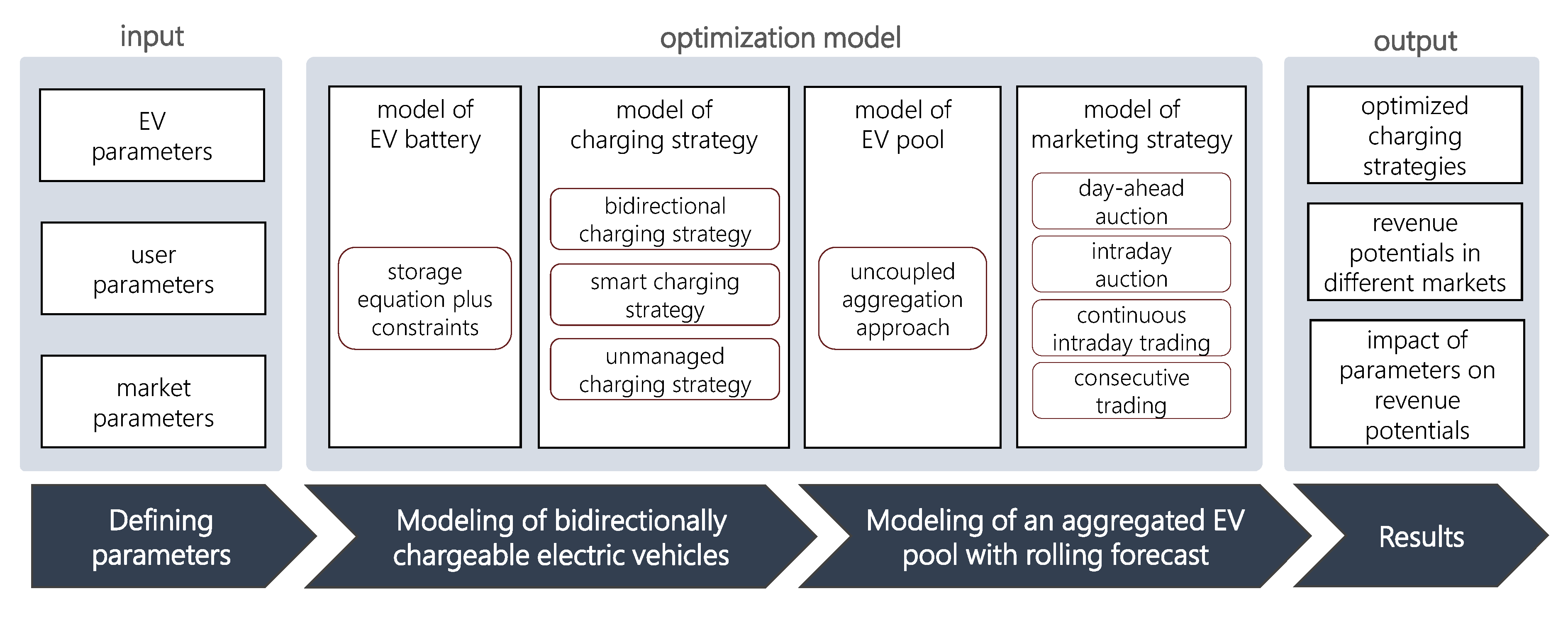
A simplified representation of the modeling process is displayed in Figure 1, where the model consists of four different parts. Based on a model of the EV’s battery, optimized charging strategies can be developed for different scenarios depending on charging and discharging restrictions. An uncoupled aggregated EV pool can be modeled to participate in different markets, where marketing strategies are optimized with a rolling forecast of market prices. The optimized strategy depends on electricity prices of the respective energy markets and is based on historical and simulated future market prices. In addition to bidirectionally chargeable EVs, two reference scenarios are considered that cover smart, unidirectionally chargeable EVs and simple, directly chargeable EVs. The entire model is implemented in Matlab, where a CPLEX solver (optimization software package) is used for optimization.
2.1. Modeling of Bidirectionally Chargeable Electric Vehicles
Modeling a bidirectionally chargeable EV consists mainly of a model of the electric battery of the vehicle similar to stationary electricity storage. The EV battery is modeled by the storage equation displayed below, which relates the state of charge (SoC) of the battery to the different amounts of electricity charged into or discharged out of the battery:
here, t stands for the modeled point in time, is the difference between two points in time and represents efficiency, which differs for the charging and discharging process. is the charging power and the discharging power at the modeled time t. The variables are considered on the alternating current side of the charging station and thus correspond to the amounts of energy traded in the market. is the sum of purchases and sales already made at the modeled time t. Accordingly, and represent the power which can be purchased or sold in the market to counteract transactions that have already taken place (countertrading). For example, purchased energy in the day-ahead market could be sold in the intraday markets resulting in a countertrade is the power, that can be used to rapidly charge the vehicle if necessary and is the EV’s energy consumption by driving at time t. The limit values of all time-dependent variables are explained in the following section. Table A1 in the Appendix A provides an overview of all these variables and their limit values.
2.1.1. State of Charge
represents the battery’s storage level at the point in time prior to the modeled point in time. The change in capacity of the battery storage corresponds to the difference from to . Due to the limited storage capacity of the electric vehicle and user requirements for a minimum storage level, the variable can assume a limited range of values.
The maximum storage level of the battery storage is limited by . If a value of 100% is set for this parameter, the entire storage capacity is available for the charging process. The minimum value varies depending on the vehicle’s location status, which is known for each point in time. Equation (2) summarizes the values that can assume:
If the vehicle is connected to the electric grid, equals . The storage level must not fall below this value or must load onto it as quickly as possible. If the vehicle is connected to a charging station and is at the point of departure, assumes the value . Before departure, the charging strategy is thus optimized in a manner such that the SoC at the time of departure at least corresponds to . If the vehicle is not connected to the electric grid, the value results in the minimum SoC.
To ensure that lies between the minimum and maximum possible storage level, Equation (3) is implemented:
where C describes the storage capacity of the electric vehicle and stands for additional, theoretical electric power to be charged. is incorporated to meet the storage level restriction in Equation (2) at any time. The possibility that the value of the storage level is below exists even if the EV is connected to the electric grid. This might occur if the storage level is lower than the minimum SoC when the vehicle arrives at a charging station or if it is not possible to charge to the minimum SoC before departure because the vehicle has not been connected for long enough. In the case that the minimum storage level cannot be reached with the charging strategy, takes on a value greater than 0 to simulate a hypothetical charging process. The variable thus can be interpreted as penalty costs that arise from the driving behavior of a user who disregards the requirements for a minimal SoC. By introducing (t), the model can optimize all driving profiles regardless of driving behavior or consumption, so that a selection of unsuitable driving profiles does not have to be made in advance. (t) is not taken into account in the storage equation and does not change the actual storage level.
2.1.2. Charging/ Discharging Power and Already Traded Energy
In the storage Equation (1), and describe the purchase and sale of power and determine the change in storage capacity for each time step. Due to the limited power of any EV charging station, the variables are limited to the maximum charging and discharging power and and to the minimum charging and discharging power and . If the vehicle is connected to a charging station, the EV battery can be charged with or discharged with . If the vehicle is not connected to the electric grid, both maximum and minimum charging and discharging power become 0.
The boolean variables and describe the state of the battery during charging and discharging processes. If a charging process takes place, is true. Analogously, the variable becomes true during discharging. Due to the fact that it is not possible to purchase and feed electricity into the electric grid at the same time, only one of the boolean variables can assume the value 1 (= true) at the modeled point in time Equation (4). A simultaneous purchase and sale in the market is, therefore, excluded.
The resulting constraints regarding these variables are shown in Equations (5) and (6):
There is a possibility that the storage capacity of the electric vehicle has already been marketed through previous trading on the electricity markets, for example through consecutive trading on different spot markets. Such traded power must be taken into account in subsequent storage optimizations. In Equations (5) and (6), and correspond to already made purchases or sales at the modeled time t. These amounts of electricity reduce the maximum charging or discharging power in such a way that only the capacity that has not yet been traded can be marketed. can be defined as the difference between and Equation (7) and is included in the storage Equation (1).
2.1.3. Countertrades
Electricity spot markets in Germany include consecutive day-ahead and intraday trading resulting in the opportunity to countertrade day-ahead purchases or sells in the intraday market. The model not only accounts for already marketed storage capacities, it also includes the possibility of compensation transactions (countertrades) that compensate for the previous trade in the opposite direction. In this regard, the variable corresponds to a buyback (counter purchase), the variable to a sellback (counter sale) of already traded storage capacities. The volume of a countertrade can at most assume the previously inversely traded amount of energy. Countertrades do not describe a physical loading or unloading process. The resulting constraints are shown in Equations (8) and (9):
Similar to the charging and discharging processes, the boolean variables and describe the state of countertrades. If a counter-purchase takes place at time t (), the EV battery cannot be discharged at the same time. Conversely, no charging process can be conducted during a counter-sale (). Equations (10) and (11) show these constraints:
2.1.4. Electricity Consumption and Fast Charging
The battery of a vehicle has an electric energy consumption at the modeled time t, which is considered in the storage equation. Due to the foresight of the driving profiles (explained in Section 2.4), EV consumption is known at all times. Each driving phase of the vehicle results in a capacity reduction.
Depending on the user’s driving behavior, it might occur that the electricity consumption of an EV is so high at one point in time that the current storage level is not sufficient to meet the energy demand, for example if the EV has not been connected to a charging station for too long. In this case, the fast charging power is utilized to comply with the restrictions of and to avoid a supposed negative storage level. The employment of the fast charging process is accompanied by an increase in storage capacity. represents the charging power at a public charging station rather than at a bidirectional charging station. The vehicle user is thus given the opportunity to charge the vehicle on the road.
2.2. Formulation of Optimization Model
The developed model of a bidirectionally chargeable EVs allows for the implementation of different optimized charging and discharging strategies, which differ in particular in the structure of the objective function. For the assessment of the use cases of arbitrage trading on the day-ahead market as well as on the intraday market, three different charging strategies are implemented: a strategy for bidirectional charging, a strategy for smart charging, and a strategy for unmanaged charging.
First, the bidirectional charging strategy, which allows for charging and discharging of the EV, is restricted to the storage equation and its aforementioned constraints. The objective of this charging strategy is to charge at minimum costs while discharging at maximum revenue. To do so, the objective function of the optimization model aims at minimizing all costs considered:
where T corresponds to the number of time steps of the optimization. Depending on the respective market, traded energy quantities per time step as well as corresponding market prices are considered. In this regard, is the price at which electricity is bought and is the price at which electricity is sold, where both prices can include respective transaction costs and possibly additional electricity price components. Charged power corresponds to a purchase transaction and is associated with costs as is each counter purchase of power. In contrast, discharged power and counter sales are traded with corresponding revenues, which is why and are subtracted.
Fast charging power and supplement power are also included in the objective function. Both fast charging costs and penalty costs are fixed to be a relatively high value, so that only the minimum necessary power is charged to meet the requirements for minimum storage level. As should only be utilized to the extent that a negative SoC is avoided, should be selected sufficiently larger than . Thus, the following condition must also be fulfilled to guarantee a functioning bidirectional charging strategy:
Second, the smart charging strategy is implemented as a reference scenario to simulate already existing smart charging stations. The objective is to minimize electricity purchase costs by intelligent charging of the EV. Since discharging the EV battery is impossible in this scenario, Equation (14) is implemented. By eliminating the discharge power, the objective function already defined via Equation (12) for the bidirectional charging strategy can also be used for the smart charging strategy.
Third, the unmanaged charging strategy accounts for today’s most commonly installed simple charging stations as a second reference scenario, where the EV battery is charged as soon as the vehicle is connected without an optimized charging control. As with the smart charging strategy, discharging is not possible Equation (14). The aim of the unmanaged charging strategy is, therefore, to maximize the storage level that is equal to minimizing the negative value of at all times. The battery is accordingly charged at maximum charging power until the battery’s storage level corresponds to or until the EV leaves the location. In addition, as for the previously explained strategies, fast charging costs and penalty costs for an insufficient SoC with regard to the location-based limit values are included. The resulting objective function is expressed as follows:
2.3. Optimization with Limited Forecast in Consecutive Spot Markets
To investigate the influence of different characteristics and requirements of the considered markets on revenue potentials of bidirectional charging, optimized trading strategies based on price forecasts are simulated by a rolling optimization model, where realistic trading behavior results from a limited foresight of market prices.
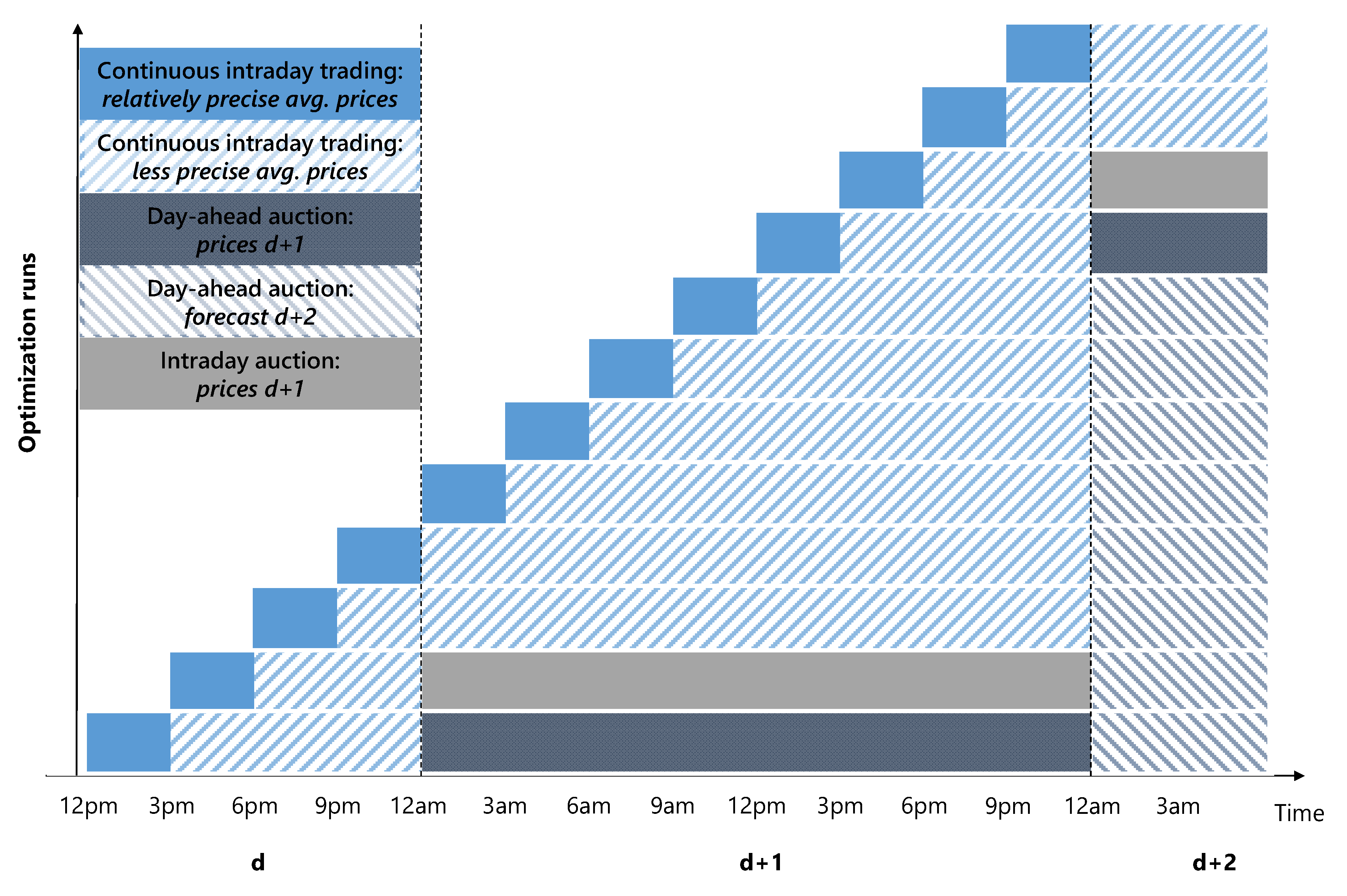
Acting in the market under uncertainty is modeled in the same manner as described in [17], where each day is divided into 8 time slices of three hours each. The model regards real trading times in the spot markets. Figure 2 illustrates the methodical procedure of consecutive trading in the day-ahead and intraday markets with rolling price forecast horizons, where each horizontal bar displays the prices known in the respective optimization run of three hours. At 12 noon of day , for instance, a market participant sees averaged continuous intraday prices of the following 12 quarter-hourly products. At the same time, less precise quarter-hourly prices of the continuous intraday are assumed for the interval from 3 pm to midnight. For day , day-ahead market prices are known and for a forecast of the day-ahead market prices is presented. The participant’s trading decision, which is the optimized marketing strategy, is based on this limited foresight.
As described by the example, foresight of market prices varies for the individual markets. Since the auction on the day-ahead market takes place daily at 12 noon for the respective following day , precise prices forecasts for are known shortly before 12 noon on day . To prevent unrealistic trading behavior at the end of day , such as discharging all batteries to maximize revenues, estimated prices for day are included in the forecast horizon, where prices are also presented at 12 noon of day . The forecast period can be one or more days representing a worse or better foresight and is evaluated in Appendix B. The length of the optimization time steps for day-ahead trading is 1 h.
For the intraday auction, precise price forecasts of day are known shortly before 3 pm of day , since the auction takes place at 3 pm. The length of the optimization time steps is 0.25 h.
Following the intraday auction, continuous intraday trading starts at 4 pm with quarter-hourly products, which defines the length of the optimization time steps. Here, a first forecast horizon of relatively precise prices is set to three hours covering the following 12 quarter-hourly products, where prices are based on trading transactions of these three hours. For the period following the three-hour time window, all continuous intraday transactions of this interval are used to calculate a second forecast price, thereby reflecting the uncertainty of market prices.
Hence, optimization runs before noon include market price information of the remaining day and the following day . The optimization runs from 12 noon on the trading day also include day . The total revenue of the marketed EV battery corresponds to the summed costs and revenues of all traded products (filled areas). The cross-hatched areas in Figure 2 are not regarded as revenues, since these are only price forecasts serving as reference points for the trading strategy.
If consecutive trading takes place in several markets, storage capacities already marketed must be taken into account in subsequent optimization runs and can be countertraded as described before. The storage level at the end of real continuous intraday trading (filled blue area) of each optimization run determines the actual charging and discharging behavior of the vehicle. This storage level is applied as the starting value for the subsequent optimization run.
2.4. Input Data and Parameterization of Electric Vehicle (EV) Pool Scenarios
In the model, parameters related to the EV are the battery’s storage capacity , charging and discharging power , and different efficiency parameters. To investigate the range of revenue potentials in detail, three different sets of EV parameters are implemented: First, a currently common-sized EV is modeled (EV1), comparable to a 2018 BMW i3 [18] and a 2018 Renault Zoe [19], using realistic values regarding storage capacity, charging and discharging power and efficiencies. Second, a relatively large EV and a highly efficient charging station are defined representing a future EV (EV2). Third, a set of ambitious, yet plausible future values is selected to model maximum revenue potentials (EV3). These parameter sets were discussed and agreed upon within the research project BCM. Table 1 summarizes the chosen parameter values for the three sets of EV models.
All losses and efficiencies considered in the model are based on discussions and on the consultation with experts from the BCM project. Other studies assume roundtrip efficiencies that are similar to EV1 [13] or slightly lower [14]. Constant values are set for the efficiencies in order to allow for a linear optimization problem, which results in much faster optimization times and thus enables many more optimization runs, i.e., more results. In real operation, however, efficiencies follow a declining, non-linear course for decreasing charging power. Hence, resulting revenue potentials of the presented model overestimate real revenues of bidirectional charging.
The user parameters result from characteristics, requirements and behavior of the vehicle user. In contrast to a large-scale stationary storage system, the battery of an EV is not continuously connected to the grid. The availability of an EV battery for V2G use cases largely depends on the individual driving profile of the user, the location of an appropriate charging station and the probability that the user has connected the vehicle to this charging station.
As a detailed representation of the driving behavior of the user, vehicle-specific driving profiles describe the EV’s whereabouts as well as its energy consumption while driving in a chronological sequence. Based on data regarding household and route information as well as individual user logbooks from the “Mobility in Germany 2017” study [20] and a methodology first developed in the MOS 2030 [21] project, annual driving profiles of various EVs are created that are available as Supplementary Materials (see Section 6). Each profile meets the following standards:
- A change of location is always accompanied by a driving phase.
- During each driving phase, the EV has discrete consumption, which leads to a reduction of the storage level.
- The EV can be located and connected either at the place of residence, the place of work or the public space
The temporal resolution of the driving profiles is quarter-hourly intervals. For each profile, the energy consumption is calculated based on information regarding driving speed, outside temperature and vehicle type.
The basic data is additionally used to cluster these driving profiles into user groups to further analyze the influence of user behavior on revenue potentials resulting in a set of commuter groups which display typical commuter behavior, and a set of non-commuter groups with homogeneous behavior different to commuter behavior. The commuter set consists of 12 commuter groups. These are defined by the time of arrival of the vehicle at the place of work and the distance traveled from the place of residence to the place of work. The non-commuter set is made up of three user groups, which are determined by age and number of persons in a household. The number of created commuter and non-commuter profiles per group reflects the real distribution within the German vehicle fleet [22]. Since revenue potentials are strongly related to driving behavior, these two different pools of driving profiles are defined as input for the model:
- a commuter pool consisting of representatives of all 12 commuter groups;
- a non-commuter pool consisting of representatives of all 3 non-commuter groups.
Table 2 summarizes the characteristics of the two pools of driving profiles including the probability of the EVs’ whereabouts, which is the averaged probability of the EV’s location at any given point in time. The sum of probability of all three locations apart from the driving phase is 94.5% for the commuter pool and 96.8% for the non-commuter pool, which represents the theoretical availability for bidirectional charging management if an appropriate charging station is installed at their location. To analyze the influence of possible charging station locations on revenue potentials of the discussed V2G use cases, the charging point location parameter can be flexibly selected in the model for each individual EV, where the distinguished three locations can be individually defined as available for bidirectional charging or not available.
The probability of each individual EV user to plug the vehicle into an available bidirectional charging station upon arrival determines the plug-in probability, where the expected value of a normally distributed probability is defined as a parameter. A higher plug-in probability results in a greater availability of the EV for V2G use cases. The parameter can be set flexibly to any value between 0% and 100%. As users will most likely be rewarded in some way for plugging in their EV, the plug-in probability is expected to be very high, up to a 100% certainty.
The parameter states the minimum storage level not to be undercut when the EV is connected to the electric grid, which guarantees a certain safety range in the event of an unscheduled departure. This parameter can be set flexibly to meet the requirements of users. The storage level that must be reached at the time of a scheduled departure, , should be adjustable by the user according to his/her preferences in a real implementation. In the model, the parameter can be set between 0% and 100%.
The charging and discharging behavior model is determined in particular by the time series of market prices. For the use cases of arbitrage trading, actual price time series of day-ahead and intraday markets from 2019 are used to represent price forecasts of a maximum of two and a half days [23,24]. For trading in the day-ahead and the intraday markets, corresponding auction prices of 2019 are used. Regarding the continuous intraday market, real prices are bilaterally determined for each transaction, where buy and sell orders are constantly matched. Thus, two representative forecast prices are determined. For the relatively precise forecast of the next three hours after modeling time t, ID3 is calculated, which is the volume-weighted quarter-hourly price of all transactions in the market for the last three hours, where market liquidity is sufficient to determine a representative market price. For the more uncertain time beyond three hours after modeling time, IDAvg is used, which is the volume-weighted quarter-hourly price of all transactions for this forecasted time horizon.
The regulatory framework for bidirectional charging applications is not yet fully defined to the point that simulated revenue potentials might determine what kind of regulatory incentive or obstacle enables or respectively prevents the considered V2G use cases. A market design with a reduction of different electricity price components such as grid fees and taxes would decrease the marginal costs of the EV accordingly and thus lead to an increased discharging behavior. To incorporate this highly important role of the market design in the model, various values are assigned to the additional charges on purchased energy parameter and resulting differences in revenues are assessed. The applied additional charges on purchased energy range from 0 €/MWh, which corresponds to a complete exemption from all additional electricity price components, to 234 €/MWh, which reflects the amount of all electricity price components for households in Germany in 2019, excluding electricity purchase prices [25].
3. Results
For the following investigations, user and EV parameters that are introduced in Section 2.4 are combined to form six EV pool scenarios (EV1, EV2, EV3 each for commuters and non-commuters). Displayed revenues of bidirectional or smart charging EVs always refer to the difference of these revenues to revenues of the unmanaged charging scenario. As long as there is no presentation explicitly showing single profile revenues, displayed revenues always refer to mean revenues of the considered EV pool scenario. User, modeling and regulatory parameters are set to the values shown in Table 3. The process of determining suitable parameters is further discussed in Section 3.3 as well as Appendix B and Appendix C.
3.1. Revenue Potentials for Vehicle-to-Grid (V2G) Use Cases
All resulting datasets in Section 3.1, individual revenue potentials depending on EV pool scenario, and driving profiles, have been made freely available (see Section 6). The following analysis shows average revenue potentials and thus represents an aggregated extract of the provided result data.
3.1.1. Revenue Potential in the German Spot Market
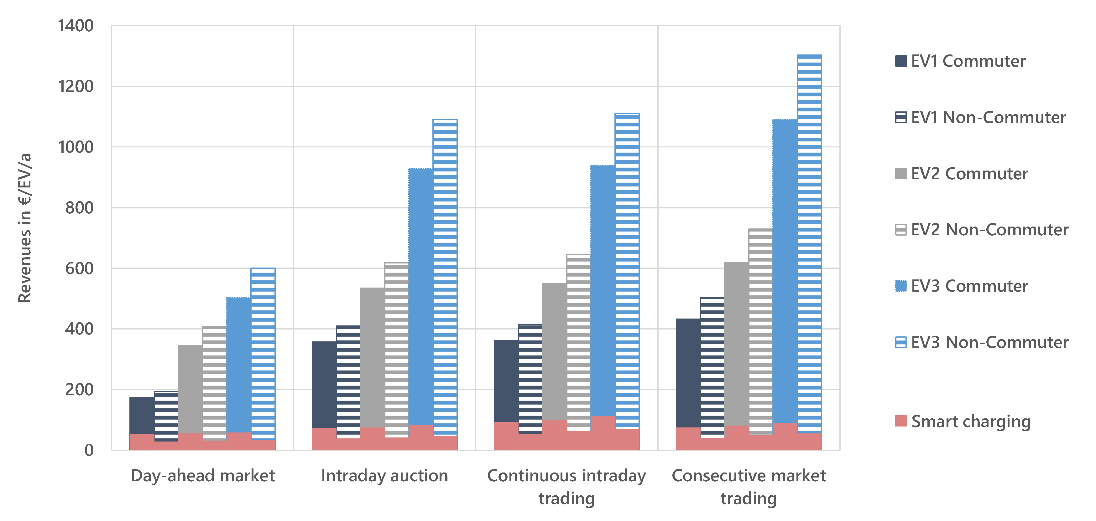
The German spot market is divided into the day-ahead auction with hourly products, the intraday auction with quarter-hourly products, and the continuous intraday trading offering quarter-hourly and hourly products. Figure 3 shows the revenue potentials for the EV pool scenarios considered in the different markets with a separate participation in the markets compared to consecutive marketing. In comparison, the revenue potential of smart charging is shown in red bars. For commuters, smart charging is more attractive than for non-commuters because of the higher annual driving and thus the higher need for charging. However, for both commuters and non-commuters arbitrage trading with bidirectional charging leads to much higher revenues compared to smart charging. Revenues of non-commuters are slightly higher than revenues of commuters due to the higher availability at the place of residence.
For trading in the day-ahead market, revenues range from almost 200 €/EV/a (EV1) to 600 €/EV/a (EV3). Quarter-hourly intraday trading leads to higher revenues due to the higher volatility in prices. Consecutive trading in the day-ahead market, the intraday auction and continuous intraday trading results in best-case revenues of 400 €/EV/a (EV1) to 1300 €/EV/a (EV3). Comparing the EV1 to EV2 pool, the 2.6 times higher capacity of EV2 implicates higher flexibility for charging and discharging times. Therefore, revenues of EV2 are 200 €/EV/a higher than the revenues of EV1. EV3 almost doubles the revenues of EV2 due to doubled charging and discharging power. The increase of charging and discharging power is, thus, even more relevant for revenue potentials than the increase of battery capacity.
3.1.2. Revenue Potential in European Markets
Since the energy systems change to a volatile and renewable production in most European countries, flexibility will be needed to cover the demand at any particular time. Therefore, bidirectionally chargeable EVs are a possible flexibility option in all European countries. To quantify revenue potentials in European countries other than Germany, we use entso-e data (European Network of Transmission System Operators for Electricity) of electricity day-ahead prices for 2019 as an input for the developed optimization model [24].
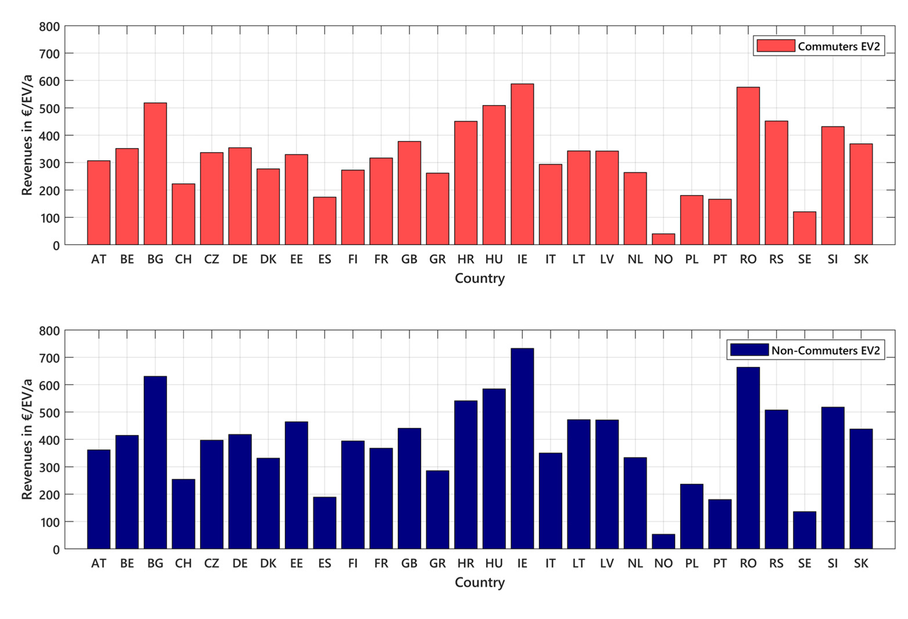
Figure 4 shows the resulting revenues for bidirectionally chargeable EVs compared to unmanaged charging for 28 European countries for commuters and non-commuters. Revenues are the highest in Ireland, Romania, Bulgaria and Hungary. These countries had scarcity prices of more than 100 €/MWh during approximately 200 h to go along with a high standard deviation of electricity prices in 2019, giving bidirectionally chargeable EVs an opportunity to use arbitrage trading more profitably. On the other hand, the revenues are the lowest for Norway and Sweden. High capacities of hydropower and some nuclear power plants in Sweden characterize the energy system in those countries [26] with almost constant marginal costs, resulting in barely volatile electricity prices.
In other countries, like Germany, Austria and France, bidirectionally chargeable EVs generate medium revenues in arbitrage trading. These energy systems are more heterogenic with some volatile renewable production as well as gas-fired, coal-fired or nuclear electricity production. Revenues in this group of countries are still varying. For example, nuclear power plants with almost constant marginal costs dominate electricity production in France [27] resulting in narrow price spreads. As another example, Austria’s energy system shows high capacities of pump storage facilities [26] resulting in flattened electricity prices. These structural characteristics lead to slightly lower revenues for bidirectionally chargeable EVs for the year 2019. On the other hand, Germany has a heterogenic production portfolio of volatile wind and solar generation as well as conventional power plants with widely varying marginal costs. Price spreads and the resulting revenues for bidirectionally chargeable EVs are thus higher there.
The structure of the energy system is consequently crucial for revenue potentials for bidirectionally chargeable EVs. In European countries, structural characteristics of electricity production differ a lot. In regard to energy transition in Europe accompanied by a shift to different volatile renewable production technologies, revenue potentials could vary even more in the future. For this reason, future revenue potentials in Germany are quantified and discussed in the following section.
3.1.3. Revenue Potential for Future Day-Ahead Market Prices
In addition to an assessment of current revenue potentials, future revenue potentials are also important for an investment in a bidirectionally chargeable EV and corresponding EV supply equipment (EVSE). For an estimation of the changed revenues, price time series for future years from the DYNAMIS project are used [28] (see Section 6). The DYNAMIS project performs a dynamic and intersectoral evaluation of measures for the cost-efficient decarbonization of the energy system. The multi-energy system model ISAaR (Integrated simulation model for unit dispatch and expansion with regionalization) determines the design of the future energy system in a model-based way to be able to evaluate the measures [29].
Based on the multi-stage, exploratory assessment of measures and packages of measures, a climate protection scenario has been developed that aims to reduce greenhouse gas emissions by 95% by 2050. This scenario is characterized on the supply side by a cost-optimized provision of energy sources and on the application side takes into account the technology- and sector-specific boundary conditions and restrictions. The expansion of renewable energies is the most important measure. Green fuels (including all solid, liquid and gaseous fuels produced from biomass, renewable electricity or a combination of both) will increasingly be used from 2040 onwards in applications that can only be electrified at considerable expense. Domestic power-to-x technologies increase the available flexibility in the electricity system due to the good storage capacity of green fuels. Bidirectionally chargeable electric vehicles are not yet modeled in this scenario path and, therefore, their effects on the energy system could not be investigated there either.
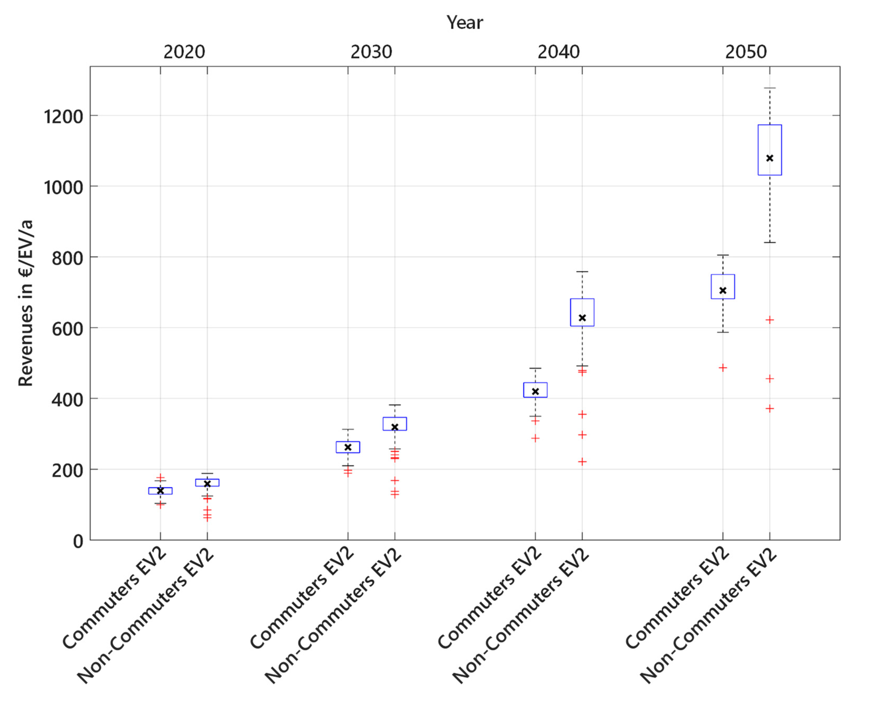
One output of the model are hourly marginal costs representing day-ahead electricity prices for the years 2020 to 2050. The mean annual day-ahead price and its daily standard deviation are shown in Table 4. It can be seen that the level and in particular the standard deviation of the electricity price increases sharply. This is mainly due to the severely changed energy system that includes high capacities of renewable energies resulting in production surpluses. This results in increasing times with electricity prices of 0 €/MWh. On the other hand, rising fuel and carbon prices many times lead to very high electricity prices due to the unavoidable use of power plants with expensive marginal costs.
The hourly price time series are transferred as input into the optimization model for bidirectionally chargeable EVs to estimate future revenue potentials in the day-ahead market. Figure 5 shows the revenues from 2020 to 2050 as a box plot. The black cross shows the mean revenues for the EVs considered. The top and bottom edges of the blue boxes indicate the 25th and 75th percentiles. The whiskers show the lowest and highest revenues, excluding outliers. Outliers that represent values that are 1.5 times bigger than the interquartile range are illustrated as red plus signs. Comparing the revenues of 2020 to those pointed out in Section 3.1.1 for 2019, mean revenues for the modeled prices are much lower than the mean revenues for the empirical data. Modeled electricity prices of energy system models often tend to be less volatile than real prices [30]. Consequently, lower price spreads lead to lower revenues.
Regarding modeled electricity prices for future years, mean revenues of bidirectionally chargeable EVs compared to unmanaged charging EVs increase by a factor of 5 to 6. This is mainly due to the future structural change of production units to renewable volatile production in combination with high carbon and fuel prices leading to many low electricity prices around 0 €/MWh and many high electricity prices. Bidirectionally chargeable EVs can harvest the resulting high price spreads to generate revenues. Another interesting aspect is the range of revenues within a user group that increases considerably in future years, showing higher uncertainty of revenue potentials. For non-commuters in particular, there is a heterogenic distribution of revenues.
The results for future electricity prices show a much higher revenue potential than for current electricity prices. Regarding these results, one has to keep in mind that there are many uncertainties about the design of the future energy system and the resulting electricity prices. Furthermore, bidirectionally chargeable EVs will have a retroactive effect on electricity prices, reducing price spreads and revenue potentials. Nevertheless, the use case of arbitrage trading for bidirectional EVs will most certainly get more attractive in future years.
3.2. Effect of V2G Use Cases on Full Cycles and Operating Hours
3.2.1. Effect of Unrestricted Trading in the Electricity Markets
The V2G use case of arbitrage trading leads to higher usage of the battery of the EVs and relevant supplying equipment as well as information and communication technology. Relevant parameters that show the additional charge of EVs are full battery cycles and total operating hours. High yearly full cycles and operating hours in particular mean a faster ageing of the battery. For the revenue modeling in Section 3.1, we deliberately applied no restrictions on cycles or operation hours. In the BCM project, a separate model will be used for evaluation of the impact of V2G use cases on EV components.
Table 5 shows the impact of the EV operation in Section 3.1.1 on the EV parameter full cycles, revenues per full cycle and operating hours. For arbitrage trading, a strong increase in full cycles by 100–500 full cycles/a and in operating hours by 1500–5000 h/a is determined. Revenues per full cycle are around 1 to 3 €/full cycle for arbitrage trading.
If one sets the highlighted parameter values in relation to currently warrantied lifetime values of lithium-ion batteries (e.g., 5000 to 6000 full cycles for residential storage systems [31,32] and a typical 10,000 operating hours in automotive applications [33]), it becomes clear that strong, relevant, additional loads of the battery arise for the use cases of arbitrage trading. These additional loads are significant, yet the use cases can still become economic without overloading the battery. Since large battery systems (as in EV2 and EV3) do not have many full cycles from driving, an alternative usage of the battery is a logical addition.
3.2.2. Effect of Restricted Trading in the Electricity Markets
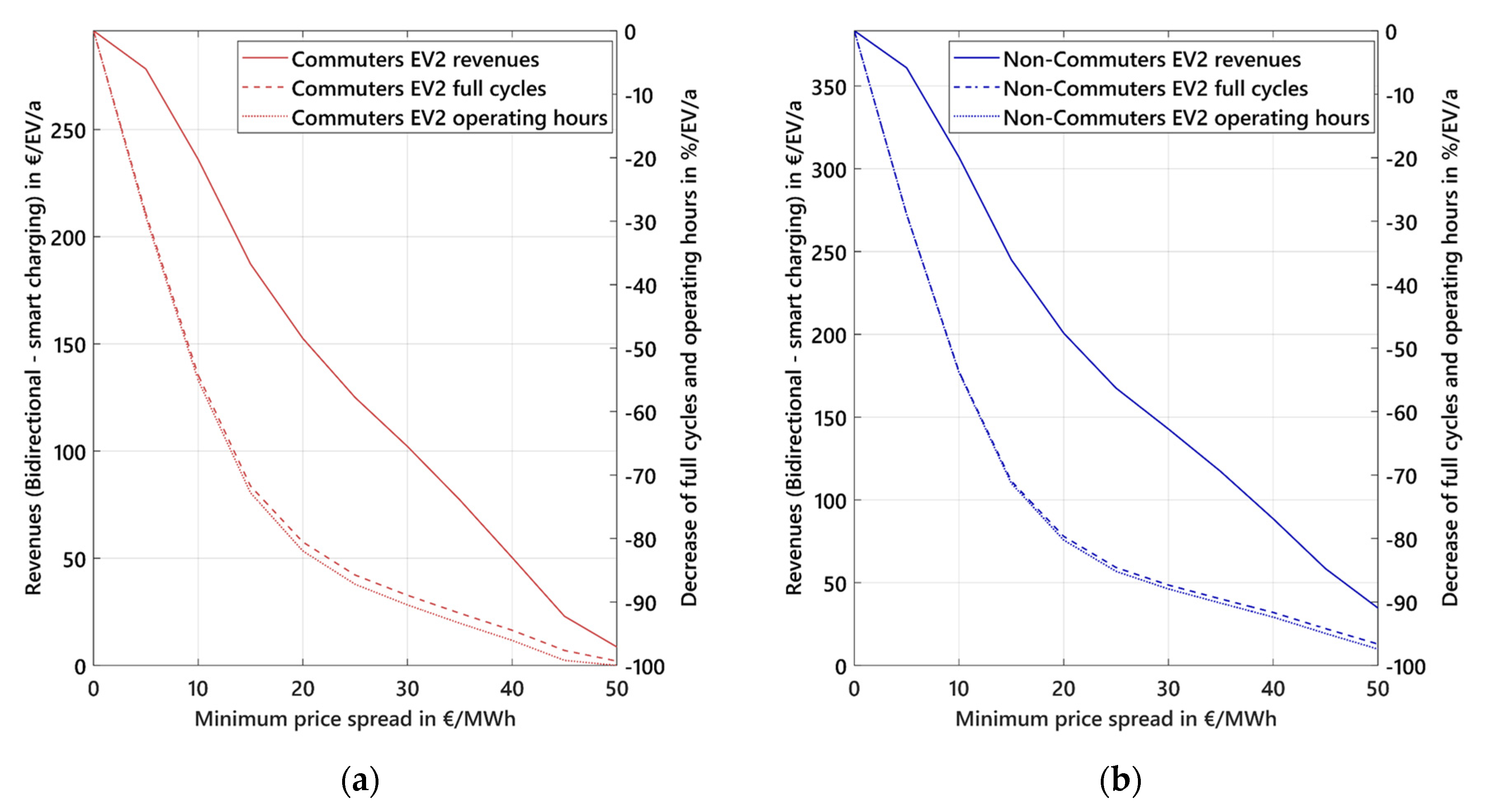
Since modeled full cycles and operating hours in the previous section could critically decrease the lifetime of the EV’s battery and power electronics, a minimum spread of electricity prices as a limit value for arbitrage trading could lower the EV’s operation while still generating high profits. The minimum spread refers to the spread of sold to purchased energy. Consequently, the selling price for these simulations has to be lowered by the minimum, modeled price spread divided by the roundtrip efficiency.
Figure 6 illustrates the effect of a minimum price spread of 0 to 50 €/MWh on full cycles and operating hours compared to revenues of EV2. Revenues refer to the difference of revenues of bidirectionally chargeable EVs to the revenues of smart charging EVs to show only the added benefit by bidirectional charging. The decrease of full cycles and operating hours is displayed in percentage referring to the simulation with no minimum price spread. The maximum decrease of full cycles and operating hours arises when increasing the minimum price spread from 0 to 5 €/MWh, whereas revenues do not decrease significantly for this change. For a minimum price spread of 10 €/MWh, additional full cycles for bidirectional charging of EV2 decrease by more than 50% to 95 full cycles per year for commuters and to 125 full cycles per year for non-commuters. For the same restriction, additional operating hours for bidirectional charging of EV2 also decrease by more than 50% to 1800 operating hours per year for commuters and to 2400 operating hours per year for non-commuters. For a minimum price spread of 10 €/MWh, revenues for both commuters and non-commuters decrease by only 20% to 240 €/EV/a and to 310 €/EV/a, respectively. By applying higher minimum price spreads, full cycles and operating hours further decrease and both the revenue per full cycle rate and revenue per operating hour rate increase. Full data for full cycles and operating hours of all EV scenarios is attached in Appendix D.
As a result, applying a minimum price spread is an effective method of limiting full cycles and operating hours while maintaining adequate profits. Even though revenues are generally decreased, this approach leads to an increase of the revenue per full cycle rate and revenue per operating hour rate and might thus represent a practicable approach for a future operation of bidirectionally chargeable EVs.
3.3. Analysis of User Parameters and Regulatory Framework on Revenue Potentials of V2G Use Cases
The revenues of bidirectional charging are determined by a multitude of input parameters. We use German day-ahead prices in 2019 (Section 3.3.1 and Section 3.3.2) as well as German intraday auction prices in 2019 (Section 3.3.2) to show the influence of user and regulatory parameters on the revenue potentials of bidirectionally chargeable EVs.
3.3.1. Influence of User Parameters
Minimum SoC at Departure
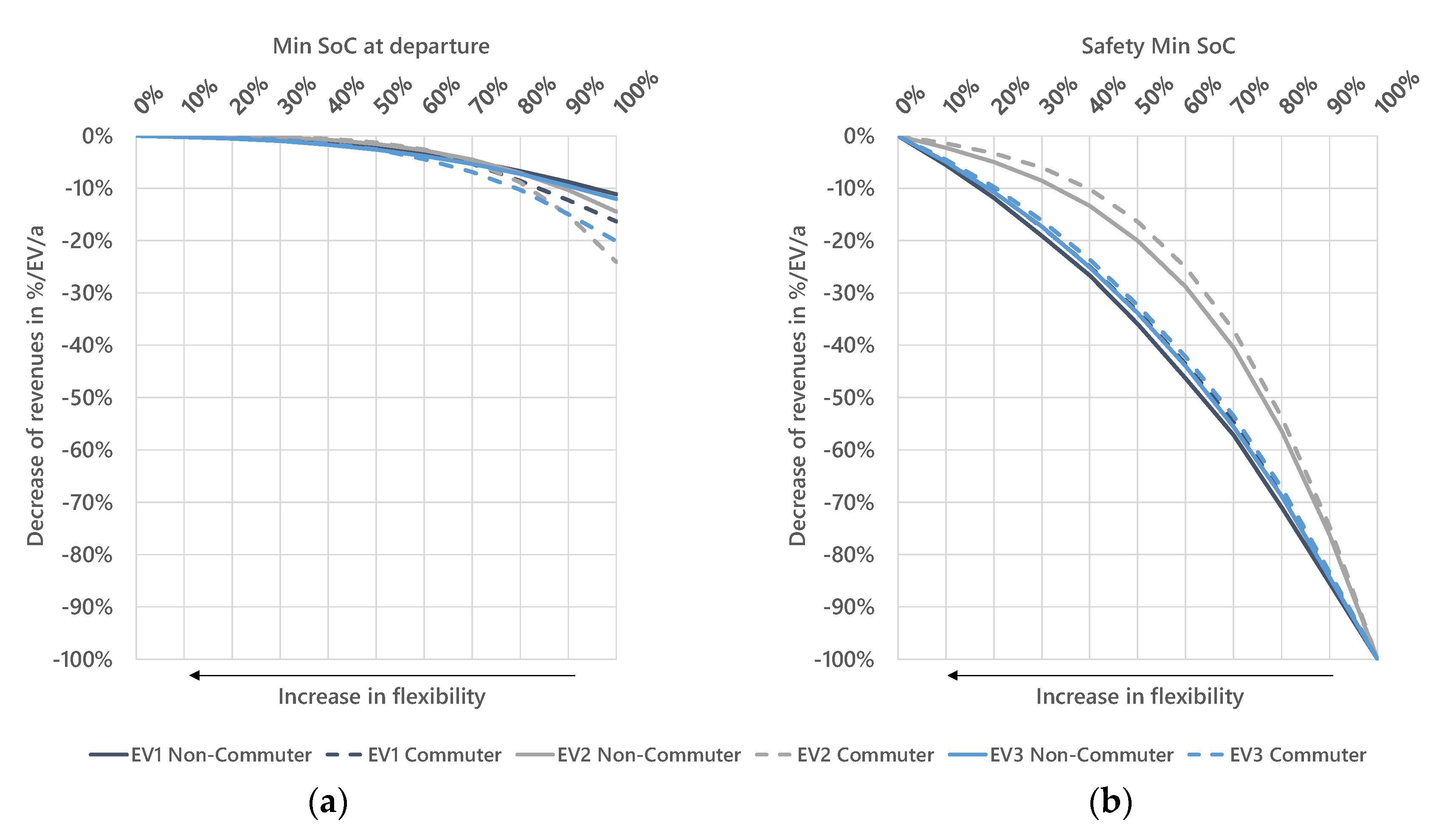
The user parameter describes the minimum battery storage level that has to be reached at a scheduled departure. Considering this restriction, a higher minimum SoC at departure leads to a reduction of flexibility regarding the bidirectional charging strategy due to the smaller range between and in which the storage level can vary. This reduces the extent to which profitable price spreads and thus a revenue-maximizing discharge behavior can be used. The effects of different parameterization of on the revenue potential in the day-ahead market are shown for the six different EV pool scenarios in Figure 7a. Potential revenues with of 10% to 100% are compared to a reference of no minimum SoC at departure ().
All scenarios show an exponential decrease in revenues with an increasing . If flexibility is gradually increased starting from a of 100% up to a of 0%, the impact on revenues is highest at the first adjustment from 100% to 90%. This is because with this first increase in flexibility, the highest electricity prices present at the considered time can be used to discharge at great profit. As low prices are used for charging, a great specific profit can be made. As flexibility is further increased due to a lower minimum SoC on departure, lower spot prices are also increasingly used for discharging. The price spread between charging and discharging decreases, which means that specific profits are reduced and revenues change less. Consequently, if an EV user can define the parameter himself, he/she should choose the lowest possible minimum SoC on departure to maximize revenues. In particular, users should avoid selecting an unnecessarily high . For investigations in this paper, a realistic minimum SoC of 70% at departure is assumed after consultation with the project BCM.
Minimum Safety SoC
The user parameter describes the minimum battery storage level that an EV always should have when connected in order to guarantee a drive to the hospital or other relevant short-distance routes at any time. If an EV arrives at a charging station with a lower SoC than , it will start charging immediately until it reaches the minimum parameterized SoC. A higher minimum safety SoC alike a higher minimum SoC at departure leads to a reduction of flexibility, since the useable capacity for marketing in the spot markets of decreases as the minimum safety SoC is increased. To quantify the impact of a minimum safety SoC, revenues with varied parameterization of are compared in Figure 7b showing the relative decrease of revenues compared to a reference with no safety SoC.
There is an exponential decrease of revenues for all EV pool scenarios depending on the minimum safety SoC. EV1 and EV3 have similar functions, while EV2 has a much smaller gradient for low safety SoCs and a steeper gradient for higher safety SoCs. This is due to the large battery capacity of EV2 and the fact, that the capacity of the charging/discharging power ratio (E/P) is much higher for EV2 at around 9, compared to the ratios of EV1 and EV3 at 3.5 and 4.5, respectively. A large battery capacity of the EV in combination with a fixed SoC on departure makes it less likely that the vehicle comes back with a low SoC on arrival and thus it is less limited by a low safety SoC than an EV with a low capacity. A low E/P ratio, on the other hand, means that EV batteries can be charged and discharged quickly with a great cycle depth, which is limited even with a low safety SOC. EV2 rarely gets these low SoCs, so a low safety SoC has little effect.
Consequently, users with EVs that have a low E/P ratio should care more about a parameterization of a very low safety SoC than users that own an EV with a higher E/P ratio. In the investigations in this paper, a minimum safety SoC of 30% for EV1 representing the status quo for BMW electric vehicles and a lower safety SoC of 20% for EV2 and EV3 representing future electric vehicles are assumed.
Plug-in Probability
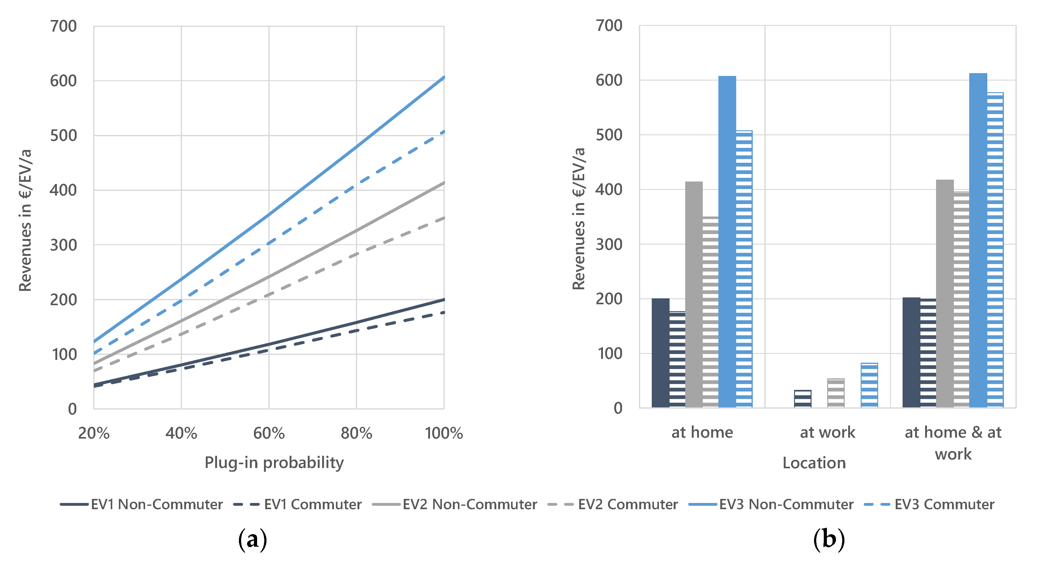
An EV user has the possibility to connect his vehicle to a charging station upon arrival at a location where a charging station is available. The probability that the user connects his vehicle to the charging station is called plug-in probability. There are several factors influencing plug-in probability. First, there is the incentive for a user to plug in his/her EV. Most importantly, the user is motivated to charge his EV for the next driving phase, where the desire could be to charge the EV directly or the possibility of smart or bidirectional charging. Since the incentives for EVs using bidirectional charging have hardly been investigated yet, there are no data on the plug-in probability of those EVs. Therefore, Figure 8a shows the influence of a changed plug-in probability on revenue potentials.
In all EV pool scenarios, there is a positive, approximately linear relationship between the plug-in probability and the revenues. If the EV is connected to a bidirectional charging station more frequently, a discharge process that maximizes revenues can be carried out more often. The gradient of the curves differs in the various scenarios. The increase in revenues in this investigation varies between 2 € for EV1 and 5 € to 6 € for EV3 with a 1% increase in the plug-in probability. Hence, for bidirectionally chargeable EVs participating in the spot markets, a higher plug-in probability means equally higher revenues. For investigations in this paper, a plug-in probability of 100% is assumed under the assumption that using bidirectional charging for arbitrage trading is profitable and users are incentivized to plug-in their EVs.
Charging Point Location
A bidirectional charging management system can only be operated if a bidirectional charging station is available at the EV’s location. In accordance with the driving profiles from Section 2.4, possible locations for the EV are the place of residence, the place of work and the public space. An extensive expansion of bidirectional charging stations in public spaces is unlikely since the main reason for using public charging stations is the fast charging of the EV. Further analysis, therefore, concentrates on charging points at the place of residence and the place of work.
Figure 8b shows the revenue potentials of bidirectionally chargeable EVs depending on the charging point location. Comparing mean revenues at the place of residence and the place of work, there is a much higher incentive even for commuters to use bidirectional charging at the place of residence for the use case of arbitrage trading. This is due to the shorter period of time spent at the place of work while restrictions for minimum safety and departure SoC still have to be regarded. EVs can be discharged profitably less frequently than at the place of residence. In the non-commuter pool, 55% of the driving profiles are never located at a place of work, which is why an evaluation is not appropriate for these vehicle pools. If charging points are located both at the place of residence and at the place of work, revenues are slightly higher than if a charging point is only available at the place of residence. Compared to total revenues, the increase is quite low.
Consequently, the revenue potential of bidirectional charging at the place of work as opposed to the place of residence is low. Bidirectional charging should, therefore, be prioritized for EV users who are ready to install a bidirectional charging station at the place of residence. In the investigations within the framework of this paper, a charging station located at or near the place of residence is assumed.
3.3.2. Impact of Regulatory Framework on Revenue Potentials
Bidirectionally chargeable EVs are a new technology whose regulatory framework conditions have not yet been developed at the European Union (EU) level [34]. An essential question is whether bidirectionally chargeable EVs are classified as storage devices and, consequently, what additional charges they have to pay for charged electricity that is discharged later.
In Germany, the wholesale market price of electricity accounts for just around 15% (around 40 to 50 €/MWh) of the price of electricity for households. The other 85% (around 260 €/MWh) of the price is accounted for by additional charges such as the EEG surcharge (surcharge of electricity for remuneration of renewables) and grid fees as well as distribution [25]. Pumped storage facilities on the other hand are exempted from most of the EEG surcharge, grid fees and other levies, so that only additional charges of around 18 €/MWh have to be paid on electricity purchases [35], which can lead to a profitable arbitrage trading for storage facilities. As most of the exemptions refer to electricity purchases, storage losses are included [36].
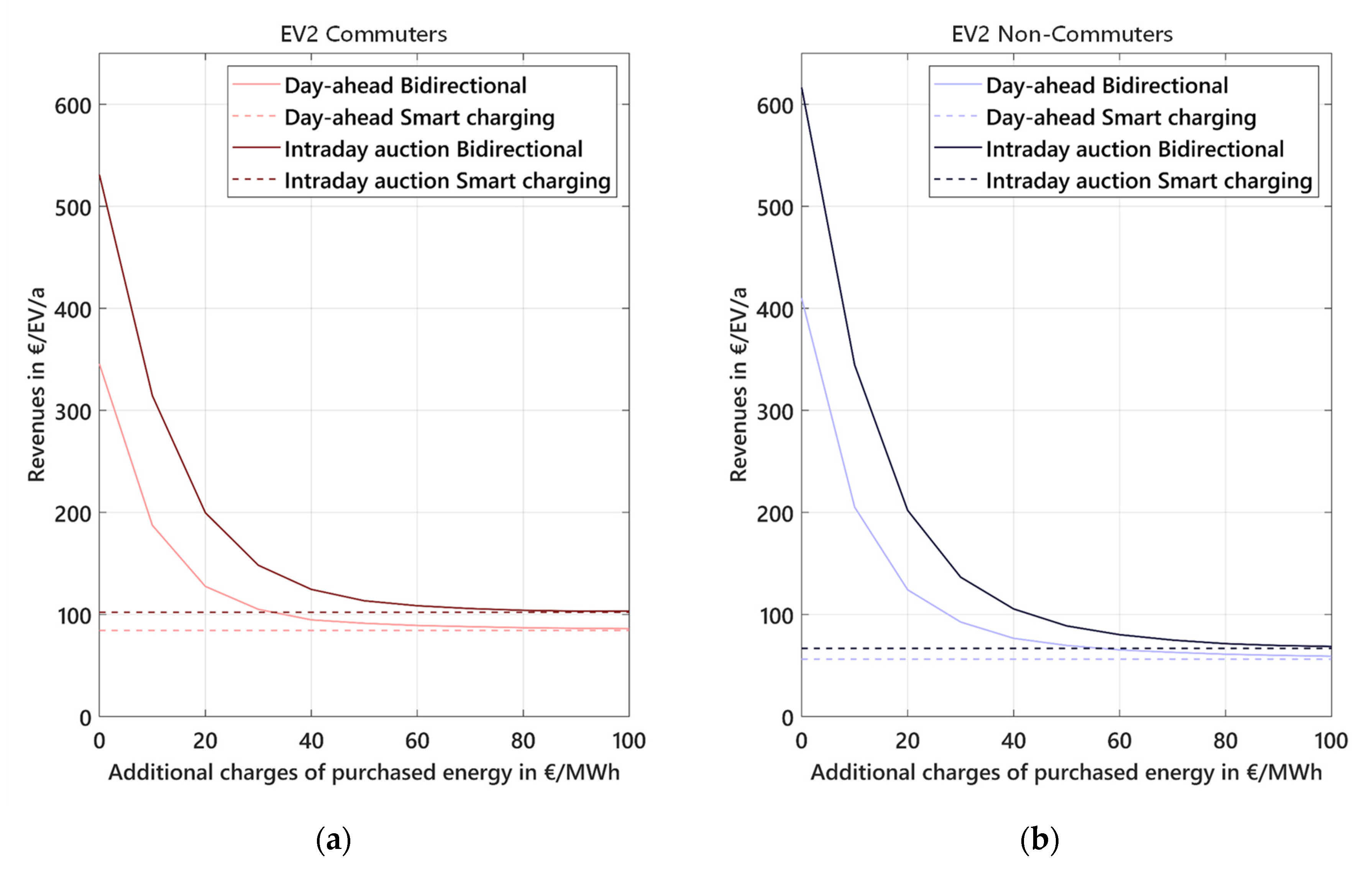
For the use case of arbitrage trading, Figure 9 shows the influence of additional charges for purchased energy in the day-ahead or intraday market on revenue potentials of bidirectionally chargeable EVs for commuters and non-commuters. The solid lines represent revenues of bidirectionally chargeable EVs compared to unmanaged charging EVs and the dashed lines show revenues of smart charging EVs compared to the unmanaged charging ones. The diagram makes clear that possible revenues are strongly dependent on the regulatory framework. Starting from mean revenues with no additional charges at around 550 to 600 €/MWh for intraday auction trading, the revenues decrease by over 40% for additional charges of only 10 €/MWh. Non-commuters have an even sharper decrease since the starting revenues are a bit higher and the minimum revenues representing smart charging are lower. Revenue potential of smart charging is higher because of the increased annual driving the associated increase in the annual charging demand. If a bidirectionally chargeable EV is regulatory-equal to a pumped storage facility with additional charges of 18 €/MWh on purchased electricity, mean revenue of non-commuters will decrease by over 60%, and commuters will have less than 50% revenue. For additional charges of more than 50 €/MWh, the added revenue of bidirectionally chargeable EVs compared to smart charging EVs is less than 20 €/EV/a.
Consequently, the future regulatory framework will decide if there is a chance for profitable arbitrage trading for bidirectional EVs. In investigations in this paper, additional costs are set to zero €/MWh to show the potential revenues for bidirectionally chargeable EVs.
4. Discussion
Bidirectionally chargeable EVs can use arbitrage trading to generate revenues for a potential improvement of their economic efficiency. Section 3.1 pointed out that revenues differ widely depending not only on the EV pool scenarios but also on the considered markets and the years under review. For an evaluation based on empirical prices of 2019 in Germany, revenues by bidirectional arbitrage trading range from 200 to 1300 €/EV/a depending on EV pool and market participation. Profits on other European day-ahead markets compared to the German day-ahead market vary between +70% and –90% and are, therefore, highly dependent on the structure of the considered energy system. For future electricity prices, there is high revenue potential for bidirectionally chargeable EVs, which is pointed out by revenues for arbitrage trading in 2050 up to six times as high as the revenue potentials determined for 2020.
Most V2G related studies in literature refer to profits in reserve markets [37,38,39]. However, some studies deal with V2G profits of arbitrage trading. Peterson et al. point out revenues of 140 to 250 US$/EV/a (120 to 210 €/EV/a) for 16 kWh EV batteries in local markets in three US cities [13]. Pelzer et al. determine 60 to 300 US$/EV/a (50 to 250 €/EV/a) depending on spatial and temporal variation in US and Singapore markets under consideration of battery degradation costs [14]. These revenues have a similar level as our calculated EV1 revenues for day-ahead trading in Germany in 2019. We do not consider battery degradation costs but show the maximization of revenues by consecutive trading in day-ahead and intraday markets and the crucial influence of user parameters and regulatory framework on revenue potentials.
Concerning analyzed user parameters, our results confirm those of Szinai et al., who found that smart charging value at residential locations is much higher than at work or public locations [40]. In addition, we found this to also be true for bidirectionally chargeable EVs. Geske et al. indicate that the minimum range and range anxiety are the most important determinants for users participating in V2G use cases [41]. In this regard, we show the quantitative effect of the parameters ‘minimum SOC at departure’ and ‘safety minimum SOC’ on the revenue potentials of bidirectionally chargeable EVs, thereby addressing the minimum range and range anxiety. Increasing these parameters leads to an exponential decrease of revenues depending on the EV type. Hence, a tradeoff exists between the users’ range anxiety and potential revenues.
With regard to the indicated high future revenues for arbitrage trading, one has to consider the retroactive effects that bidirectional EVs participating in the considered markets will have on market prices. As for arbitrage trading, where EVs charge when spot prices are low and discharge when spot prices are high, a flattening impact on spot prices is foreseeable. From a spot market perspective, offers of electric energy increase during times of high spot prices, and the demand for electricity increases during times of low prices, leading to higher prices when prices are low and lower prices when prices are high. These retroactive effects will lower revenue potentials if significant quantities of bidirectionally chargeable EVs participate in the markets. For quantitative evaluation of these retroactive effects, an energy system model is needed that models the supply and demand curves and thus can model price changes attributable to bidirectionally chargeable EVs. This additional research will be addressed by the BCM project in a following publication.
For an assessment of the impact of bidirectionally chargeable EVs in the markets, Table 6 shows the market volumes of considered and relevant markets and fitting EV quantities with 10 kW bidirectional charging station that would cover the market completely. Regarding the table and considering Germany’s aim of 10 million EVs by 2030, the probable retroactive effect in the markets can be derived. If a significant quantity of those EVs will have a bidirectional charging station and use V2G, there will be a high impact on prices in the intraday auction, and the quarter-hourly and the hourly continuous intraday trading market. A lower retroactive effect will occur for day-ahead prices in the German spot market.
Besides restrictions of market volumes, Section 3.2 points out the effect of V2G use cases on full cycles and operating hours of the EV’s battery storage. For the use case of arbitrage trading, there is a high increase in battery usage resulting in an accelerated ageing of the battery. Although warranties for the full cycle lifetime of battery systems increase, the additional charge on the battery will reduce the use case’s economic efficiency. However, in Section 3.2.2, we point out that both full cycles and operating hours can be decreased significantly, while revenues are still high by implementing a minimum price spread for arbitrage trading. In the BCM project, a detailed battery-ageing model is used for evaluating the impact of V2G on the battery and power electronics of the EV.
Another important restriction is the regulatory framework. Section 3.3.2 has shown the immense effect of additional charges on the profitability of the use case of arbitrage trading. It will be decisive if bidirectionally chargeable EVs are regulatory classified as a storage and if so, which additional charges will arise.
Regarding model limitations, constant values are set for the efficiencies of charging and discharging in order to achieve much faster optimization times. For arbitrage trading, charging and discharging processes usually use the highest possible power as price signals express either purchasing, selling or doing nothing. In a following publication in the BCM project, revenues of vehicle-to-home (V2H) use cases are compared by using constant and non-constant efficiencies, in which it is pointed out that modeling a non-constant efficiency for V2H use cases is necessary.
For the use case of arbitrage trading, we model revenues without perfect foresight for a rolling horizon of two to three days. The implemented market prices are real and not forecasted prices, which are used for real trading. On the other hand, it can be assumed that price forecasts over- and underestimated actual market prices to the same extent and on an average alignment with real market prices resulting in a realistic modeling of revenues for bidirectionally chargeable EVs.
Finally, for the evaluation of the economy of V2G use cases, additional costs have to be considered. The main additional hardware costs result from a bidirectional charging station. Currently, the cost for the only bidirectional charging station soon available in the German market is around 6000 € [43]. Medium-term cost projections in the project BCM for a bidirectional charging station is around 2000 €. In regard to the current stage of the BCM project, cost projections for additional hardware and operating costs are not defined, and the economic efficiency of the use cases can, therefore, not yet be evaluated.
5. Conclusions
Based on the developed aggregated storage optimization model, revenues of bidirectionally chargeable EVs have been calculated for the V2G use case arbitrage trading. As a detailed description of optimization constraints and input data are provided, readers are able to reconstruct the indicated revenues of bidirectionally chargeable EVs. The major findings of this research are:
- We developed a rolling optimization model that regards real trading times of European spot markets and allows countertrading in consecutive traded markets while considering user behavior parameters leading to a realistic representation of revenue potentials of bidirectionally chargeable EVs using arbitrage trading.
- Revenues of bidirectionally chargeable EVs are dependent on user parameters. An increase of the safety minimum SoC at the place of residence or the minimum SoC at departure leads to an exponential decrease of revenues for bidirectionally chargeable EVs.
- For a participation of bidirectionally chargeable EVs in the German spot markets in 2019, potential revenues range from 200 to 1300 €/EV/a depending on the modeled EV pool scenario under the assumption of no additional charges for purchased electricity.
- Revenues of currently available EV models participating in the day-ahead market are comparable to findings of other literature, while our research shows a significant increase in revenues for consecutive trading in all spot markets.
- The regulatory framework concerning additional charges of purchased energy is the most decisive parameter for the potential revenues of bidirectionally chargeable EVs.
- Considering additional charges amounting for example to the payments of a pumped storage facility for bidirectionally chargeable EVs results in a decrease of revenues by 50% to 60%. Thus, if V2G arbitrage trading is supposed to give flexibility to the future energy system, the market regulator will have to exempt bidirectionally chargeable EVs from the major part of additional charges.
- Unrestricted arbitrage trading of bidirectionally chargeable EVs results in a sharp increase of full cycles and operating hours by 200 to 600 full cycles/a, respectively, by 2000 to 6000 h/a resulting in much faster battery degradation. Restricted arbitrage trading with a minimum price spread can lower this additional load for EV and EVSE. For a minimum price spread of 10 €/MWh, operating hours and full cycles decrease by 50% while revenues only decrease by 20%.
- Revenues of bidirectionally chargeable EVs differ widely depending on the electricity production structure of the energy system. European day-ahead market revenues for EV2 in 2019 range from 50 €/EV/a in Norway to 700 €/EV/a in Ireland. Modeled potential future revenues are 2 times higher in 2030 and 5 to 6 times higher in 2050 than modeled revenues in 2020.
In general, potentially high revenue opportunities are identified for bidirectionally chargeable EVs in the electricity markets. Thus, participating in V2G use cases could promote electric mobility and, thereby, provide the flexibility needed for the energy system of the future. For future profitable usage of V2G use cases, the design of the regulatory framework and battery lifetime are decisive. For further investigations, especially retroactive effects of bidirectionally chargeable EVs on market prices and resulting decrease of revenue opportunities is of interest.
6. Data Availability
The driving profile data are available in Supplementary Materials ‘input and results data\driving profiles’. The modelled future electricity prices are available in ‘https://openenergy-platform.org/dataedit/view/scenario/ffe_dynamis_emission_factors_marginal_cost’.
In Section 3.1 which analyzed revenue potentials of individual EVs for German spot market prices, European day-ahead market prices and future day-ahead market prices are available in Supplementary Materials ‘input and results data\revenues_Section_3_1’.
Supplementary Materials
The following are available online at https://www.mdpi.com/1996-1073/13/21/5812/s1, Driving Profiles data: 50 commuter and 75 non-commuter driving profiles including quarter-hourly resolved time series for location and consumption of individual EVs: http://opendata.ffe.de/dynamis-emission-factors, Revenues Section 3.1: Individual user revenues depending on driving profiles as additional data for shown aggregated revenues in Section 3.1.
Author Contributions
Conceptualization, T.K.; Data curation, T.K.; Formal analysis, T.K. and P.D.; Investigation, T.K.; Methodology, T.K. and P.D.; Software, T.K.; Validation, T.K.; Visualization, T.K.; Writing—original draft, T.K. and P.D.; Writing—review & editing, T.K., P.D. and S.v.R. All authors have read and agreed to the published version of the manuscript.
Funding
The described work is conducted within the project BCM by Forschungsgesellschaft für Energiewirtschaft mbH and funded by Bundesminsterium für Wirtschaft und Energie (BMWi) under the funding code 01MV18004C.
Conflicts of Interest
The authors declare no conflict of interest. The funders had no role in the design of the study; in the collection, analyses, or interpretation of data; in the writing of the manuscript; or in the decision to publish the results.
Appendix A

Table A1.
List of time-dependent variables of the storage equation and their respective limit values.
Table A1.
List of time-dependent variables of the storage equation and their respective limit values.
| Time-Dependent Variables | Minimum Value | Maximum Value | |
|---|---|---|---|
| State of charge | |||
| Charging power | |||
| Discharging power | |||
| Discharging boolean | 0 | 1 | |
| Charging boolean | 0 | 1 | |
| Counter purchase power | 0 | ||
| Counter sale power | 0 | ||
| Counter purchase boolean | 0 | 1 | |
| Counter sale boolean | 0 | 1 | |
| Supplementary power | 0 | ∞ | |
| Fast charging power | 0 | ∞ | |
Appendix B
Influence of Forecast Period
For modeling realistic revenues of bidirectionally chargeable EVs, a rolling, limited time horizon is implemented. The selected limited time horizon is important for two reasons. Firstly, market prices are perfectly forecasted, which leads to a perfect EV charging strategy for the considered time horizon. As an example, if there are very low prices 10 days ahead of the starting point, the EV may shift its charging in the future. In reality, the low prices may depend on renewable energies that cannot be forecast 10 days in advance accurately. Secondly, EV driving behavior is perfectly forecast. In reality, regular driving (e.g., commuting to work) can be predicted most of the time, whereas more spontaneous driving (e.g., for free time activities) is much more uncertain. In this regard, it is hard to declare a realistic horizon for forecasting in the model.
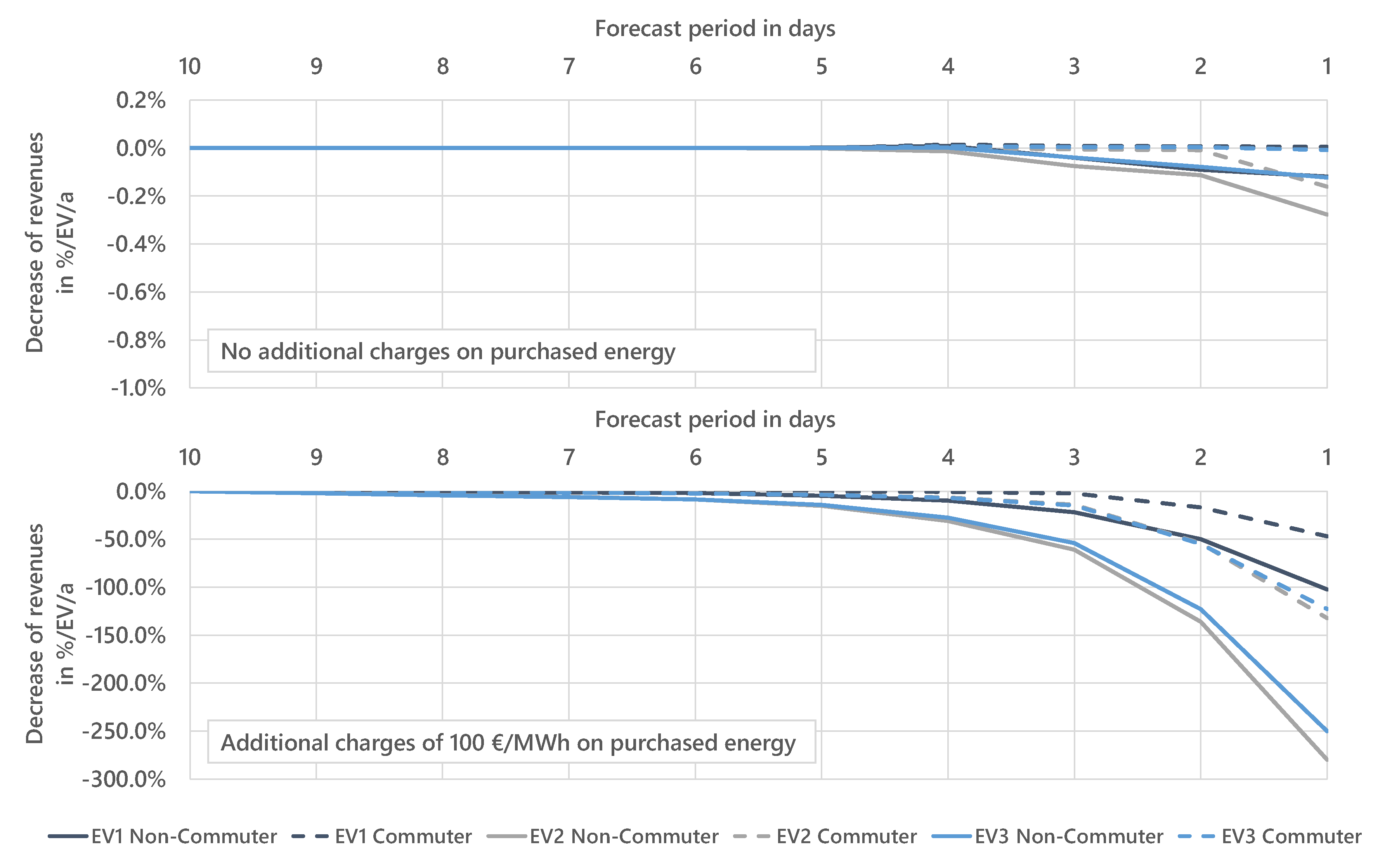
The upper diagram in Figure A1 illustrates the effect of an adapted forecasting period on revenue potentials of bidirectionally chargeable EVs with no additional charges on purchased energy. Starting from a forecast horizon of ten days going down to four days, there is no change in revenues. A shorter forecast period results in slightly decreased revenues, but the impact of the forecast period on revenues is very low. This is mainly due to daily characteristics of the electricity price. Price spreads are used to charge with low prices and discharge with high prices with just a slight dependence on future departures or future electricity prices. Depending on the regulatory framework, additional charges can arise for purchased energy. The bottom diagram shows the effect of a varied forecast horizon on the revenues with additional charges of 100 €/MWh on purchased energy. There is huge decrease of revenues even resulting in negative revenues for short forecast periods, since EVs often do not know a future departure and consequently discharge although the future charging price is much higher. Only for forecast periods of 7 days and longer are revenues relatively stable compared to a horizon of 10 days.
The forecast horizon is mainly applied to prevent unrealistic future trading after the optimized period that is remunerated. For simulations with no additional charges, the rolling optimization is still necessary as it allows consideration of real sequential market trading. Consequently, for investigations in this paper a short forecast period of one day is defined. For an evaluation of the regulatory framework in Section 3.3.2, a longer forecast period of seven days is applied to prevent unrealistic discharging although charging prices are higher.
Figure A1.
Influence of forecasting horizon on revenue potentials of bidirectionally chargeable EVs for the use cases of arbitrage trading with no additional charges (top) and additional charges of 100 €/MWh (bottom) on purchased energy.
Figure A1.
Influence of forecasting horizon on revenue potentials of bidirectionally chargeable EVs for the use cases of arbitrage trading with no additional charges (top) and additional charges of 100 €/MWh (bottom) on purchased energy.

Appendix C
Determination of a Realistic Pool Size
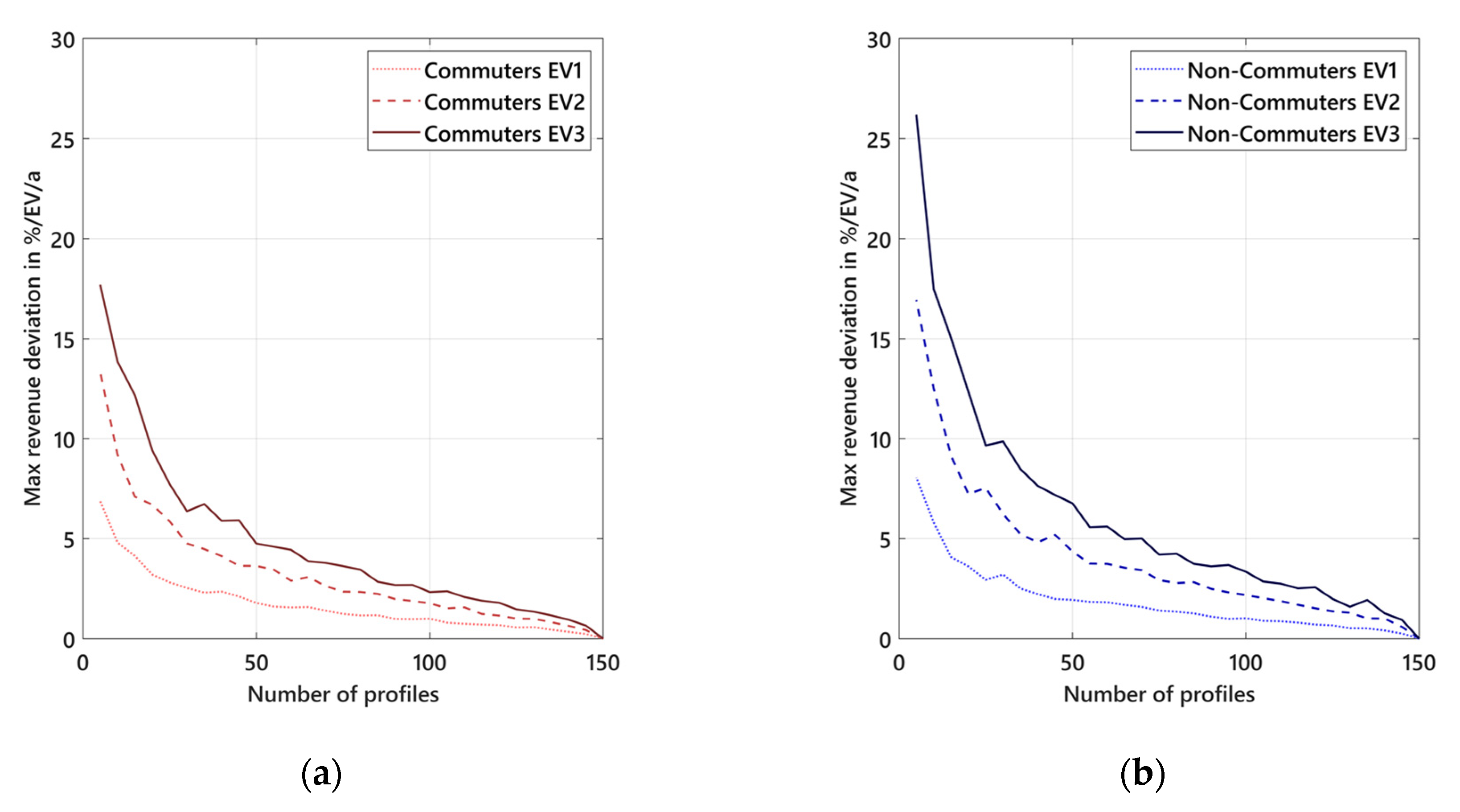
The modeling of a realistic vehicle pool is characterized by the EV pool size. The revenue potential of bidirectional charging of a single vehicle depends strongly on the individual driving profile of the user. In order to show a meaningful average revenue potential for different EV pool groups, a relevant number of vehicles must be determined for the model calculations. As computational time is linearly dependent on the number of profiles considered, a trade-off has to be faced. The aim of the investigations is to identify a pool size at which the addition of further vehicles has a low influence on revenues compared to the higher computational time. For all evaluated EV pool scenarios, the revenue potential on the German day-ahead market in 2019 was investigated for different pool sizes. For 5 to 150 profiles, a random drawing of 50,000 profile groups leads to a statistically significant analysis. Figure A2 shows the maximum revenue deviation for different numbers of profiles compared to the best case of 150 profiles. The maximum number of individual profiles is 150 in order to limit computational time. If all 150 profiles are drawn, there will be no revenue deviation to the best case of 150 profiles.
Figure A2.
Maximum revenue deviation for a varying number of profiles compared to the best case of 150 profiles for a drawing of 50,000 EV profile groups for commuters (a) and non-commuters (b).
Figure A2.
Maximum revenue deviation for a varying number of profiles compared to the best case of 150 profiles for a drawing of 50,000 EV profile groups for commuters (a) and non-commuters (b).

The more vehicles that are modeled, the less is the maximum revenue deviation. A relevant pool size for the EV pool scenarios can be determined by the revenue difference falling below a defined threshold value. A maximum deviation of less than 5% per vehicle per year is assumed to be sufficiently accurate while limiting computational time. This results in a relevant pool size of 50 vehicles for a commuter EV pool. A representative non-commuter EV pool needs a number of 75 vehicles. Revenues of non-commuters are more heterogenic than revenues of commuters because commuters have a more regular driving profile during weekdays.
Appendix D
Table A2.
Revenues, full cycles and operating hours for all EV scenarios (difference of bidirectional charging to smart charging) with restricted minimum price spread.
Table A2.
Revenues, full cycles and operating hours for all EV scenarios (difference of bidirectional charging to smart charging) with restricted minimum price spread.
| EV1—Commuter | ||||||
|---|---|---|---|---|---|---|
| Minimum Price spread in €/MWh | Revenues in €/EV/a | Full Cycles per Year | Operating Hours per Year | Average Price Spread in €/MWh | Revenue/ Full Cycle in €/Full Cycle | Revenue/ Operating Hour in €/Operating Hour |
| 0 | 125.1 | 231.0 | 1898 | 14.2 | 0.54 | 0.07 |
| 5 | 117.7 | 166.7 | 1363 | 18.6 | 0.71 | 0.09 |
| 10 | 97.8 | 102.9 | 841 | 25.0 | 0.95 | 0.12 |
| 15 | 75.5 | 60.4 | 494 | 32.9 | 1.25 | 0.15 |
| 20 | 59.7 | 38.7 | 319 | 40.6 | 1.54 | 0.19 |
| 25 | 46.2 | 25.6 | 210 | 47.4 | 1.80 | 0.22 |
| 30 | 37.1 | 18.6 | 153 | 52.6 | 2.00 | 0.24 |
| 35 | 27.7 | 13.1 | 109 | 55.7 | 2.12 | 0.25 |
| 40 | 17.2 | 8.0 | 67 | 56.8 | 2.16 | 0.26 |
| 45 | 6.6 | 2.8 | 24 | 62.9 | 2.39 | 0.27 |
| 50 | 2.7 | 0.9 | 7 | 77.2 | 2.93 | 0.35 |
| EV1—Non-Commuter | ||||||
| Minimum Price Spread in €/MWh | Revenues in €/EV/a | Full Cycles per Year | Operating Hours per Year | Average Price Spread in €/MWh | Revenue/ Full Cycle in €/Full Cycle | Revenue/ Operating Hour in €/Operating Hour |
| 0 | 173.3 | 324.2 | 2737 | 14.1 | 0.53 | 0.06 |
| 5 | 162.5 | 226.7 | 1911 | 18.9 | 0.72 | 0.08 |
| 10 | 135.6 | 139.5 | 1173 | 25.6 | 0.97 | 0.12 |
| 15 | 107.1 | 85.0 | 712 | 33.2 | 1.26 | 0.15 |
| 20 | 86.1 | 56.1 | 472 | 40.4 | 1.54 | 0.18 |
| 25 | 68.7 | 38.8 | 327 | 46.6 | 1.77 | 0.21 |
| 30 | 56.5 | 29.0 | 245 | 51.3 | 1.95 | 0.23 |
| 35 | 44.2 | 22.1 | 189 | 52.7 | 2.00 | 0.23 |
| 40 | 33.7 | 16.5 | 140 | 53.9 | 2.05 | 0.24 |
| 45 | 19.9 | 10.1 | 87 | 51.9 | 1.97 | 0.23 |
| 50 | 10.8 | 5.5 | 48 | 51.4 | 1.95 | 0.23 |
| EV2—Commuter | ||||||
| Minimum Price Spread in €/MWh | Revenues in €/EV/a | Full Cycles per Year | Operating Hours per Year | Average Price Spread in €/MWh | Revenue/ Full Cycle in €/Full Cycle | Revenue/ Operating Hour in €/Operating Hour |
| 0 | 296.1 | 211.4 | 3963 | 14.0 | 1.40 | 0.07 |
| 5 | 278.2 | 150.5 | 2819 | 18.5 | 1.85 | 0.10 |
| 10 | 236.1 | 96.8 | 1815 | 24.4 | 2.44 | 0.13 |
| 15 | 187.3 | 59.9 | 1123 | 31.3 | 3.13 | 0.17 |
| 20 | 152.5 | 41.3 | 766 | 37.0 | 3.70 | 0.20 |
| 25 | 125.0 | 30.3 | 561 | 41.3 | 4.13 | 0.22 |
| 30 | 102.1 | 23.5 | 434 | 43.4 | 4.34 | 0.24 |
| 35 | 77.2 | 17.5 | 322 | 44.0 | 4.40 | 0.24 |
| 40 | 50.3 | 11.9 | 216 | 42.3 | 4.23 | 0.23 |
| 45 | 22.9 | 5.2 | 93 | 44.3 | 4.43 | 0.25 |
| 50 | 8.6 | 1.6 | 30 | 52.9 | 5.29 | 0.29 |
| EV2—Non-Commuter | ||||||
| Minimum Price Spread in €/MWh | Revenues in €/EV/a | Full Cycles per Year | Operating Hours per Year | Average Price Spread in €/MWh | Revenue/ Full Cycle in €/Full Cycle | Revenue/ Operating Hour in €/Operating Hour |
| 0 | 383.4 | 270.7 | 5113 | 14.2 | 1.42 | 0.07 |
| 5 | 361.0 | 192.5 | 3645 | 18.8 | 1.88 | 0.10 |
| 10 | 307.0 | 125.4 | 2383 | 24.5 | 2.45 | 0.13 |
| 15 | 245.0 | 78.7 | 1498 | 31.1 | 3.11 | 0.16 |
| 20 | 200.7 | 55.2 | 1045 | 36.4 | 3.64 | 0.19 |
| 25 | 167.5 | 41.9 | 795 | 40.0 | 4.00 | 0.21 |
| 30 | 142.8 | 34.5 | 654 | 41.5 | 4.15 | 0.22 |
| 35 | 117.1 | 28.5 | 541 | 41.0 | 4.10 | 0.22 |
| 40 | 88.6 | 22.8 | 429 | 38.9 | 3.89 | 0.21 |
| 45 | 58.5 | 15.9 | 299 | 36.8 | 3.68 | 0.20 |
| 50 | 34.7 | 9.3 | 174 | 37.3 | 3.73 | 0.20 |
| EV3—Commuter | ||||||
| Minimum Price Spread in €/MWh | Revenues in €/EV/a | Full Cycles per Year | Operating Hours per Year | Average Price Spread in €/MWh | Revenue/ Full Cycle in €/Full Cycle | Revenue/ Operating Hour in €/Operating Hour |
| 0 | 451.2 | 301.4 | 2994 | 15.0 | 1.50 | 0.15 |
| 5 | 430.6 | 227.5 | 2243 | 18.9 | 1.89 | 0.19 |
| 10 | 369.2 | 151.5 | 1487 | 24.4 | 2.44 | 0.25 |
| 15 | 290.4 | 92.4 | 898 | 31.4 | 3.14 | 0.32 |
| 20 | 231.8 | 60.6 | 582 | 38.3 | 3.83 | 0.40 |
| 25 | 187.6 | 42.6 | 402 | 44.0 | 4.40 | 0.47 |
| 30 | 152.0 | 31.9 | 297 | 47.7 | 4.77 | 0.51 |
| 35 | 123.6 | 24.5 | 227 | 50.4 | 5.04 | 0.54 |
| 40 | 85.1 | 17.1 | 156 | 49.8 | 4.98 | 0.55 |
| 45 | 41.7 | 8.5 | 75 | 49.2 | 4.92 | 0.55 |
| 50 | 16.7 | 2.8 | 25 | 59.1 | 5.91 | 0.66 |
| EV3—Non-Commuter | ||||||
| Minimum Price Spread in €/MWh | Revenues in €/EV/a | Full Cycles per Year | Operating Hours per Year | Average Price Spread in €/MWh | Revenue/ Full Cycle in €/Full Cycle | Revenue/ Operating Hour in €/Operating Hour |
| 0 | 574.6 | 397.5 | 3979 | 14.5 | 1.45 | 0.14 |
| 5 | 545.8 | 291.1 | 2913 | 18.8 | 1.88 | 0.19 |
| 10 | 466.9 | 191.4 | 1916 | 24.4 | 2.44 | 0.24 |
| 15 | 370.3 | 118.3 | 1188 | 31.3 | 3.13 | 0.31 |
| 20 | 298.4 | 79.2 | 795 | 37.7 | 3.77 | 0.38 |
| 25 | 243.9 | 56.8 | 568 | 42.9 | 4.29 | 0.43 |
| 30 | 202.6 | 44.2 | 444 | 45.9 | 4.59 | 0.46 |
| 35 | 171.8 | 36.2 | 365 | 47.5 | 4.75 | 0.47 |
| 40 | 132.8 | 28.4 | 287 | 46.7 | 4.67 | 0.46 |
| 45 | 92.3 | 20.7 | 211 | 44.6 | 4.46 | 0.44 |
| 50 | 56.0 | 12.7 | 128 | 44.1 | 4.41 | 0.44 |
References
- BMU. Klimaschutz in Zahlen—Fakten, Trends und Impulse deutscher Klimapolitik; BMU: Berlin, Germany, 2018.
- Fattler, S.; Regett, A. Environmental Impact of Electric Vehicles: Influence of Intelligent Charging Strategies. In Grid Integration of Electric Mobility 2019; Forschungsstelle für Energiewirtschafte e.V: München, Germany, 2019. [Google Scholar]
- European Comission. A Clean Planet for All –A European Strategic Long-Term Vision for A Prosperous, Modern, Competitive and Climate Neutral Economy; European Commission: Brussels, Belgium, 2018. [Google Scholar]
- Hinterstocker, M.; Ostermann, A.; Muller, M.; Dossow, P.; von Roon, S.; Kern, T.; Pellinger, C. Bidirectional Charging Management—Field Trial and Measurement Concept for Assessment of Novel Charging Strategies; Forschungsstelle für Energiewirtschaft e.V.: München, Germany, 2019. [Google Scholar]
- Pham, T. Do German renewable energy resources affect prices and mitigate market power in the French electricity market? Appl. Econ. 2019, 51, 1–14. [Google Scholar] [CrossRef]
- EPEX SPOT SE. Trading on EPEX SPOT; EPEX SPOT SE: Paris, France, 2019. [Google Scholar]
- Illing, B.; Warweg, O. Analysis of international approaches to integrate electric vehicles into energy market. In Proceedings of the 12th International Conference on the European Energy Market (EEM), Lisbon, Portugal, 19–22 May 2015. [Google Scholar]
- Shafiullah, M.; Al-Awami, A.T. Maximizing the profit of a load aggregator by optimal scheduling of day ahead load with EVs. In Proceedings of the 2015 IEEE International Conference on Industrial Technology (ICIT), Seville, Spain, 17–19 March 2015. [Google Scholar]
- Illing, B.; Warweg, O. Achievable revenues for electric vehicles according to current and future energy market conditions. In Proceedings of the 13th International Conference on the European Energy Market (EEM), Porto, Portugal, 6–9 June 2016. [Google Scholar]
- Bessa, R.J.; Matos, M.A.; Soares, F.J.; Lopes, J.A.P. Optimized Bidding of a EV Aggregation Agent in the Electricity Market. IEEE Trans. Smart Grid 2011, 3, 443–452. [Google Scholar] [CrossRef]
- Rominger, J.; Losch, M.; Steuer, S.; Koper, K.; Schmeck, H. Analysis of the German Continuous Intraday Market and the Revenue Potential for Flexibility Options; IEEE: Piscataway, NJ, USA, 2019. [Google Scholar]
- Schmidt, R.; Schnittmann, E.; Meese, J.; Dahlmann, B.; Zdrallek, M.; Armoneit, T. Revenue-Optimized Marketing of Electric Vehicles’ Flexibility Options; IEEE: Piscataway, NJ, USA, 2019. [Google Scholar]
- Peterson, S.B.; Whitacre, J.; Apt, J. The Economics of Using Plug-In Hybrid Electric Vehicle Battery Packs for Grid Storage; RELX Group: London, UK, 2009. [Google Scholar]
- Pelzer, D.; Ciechanowicz, D.; Knoll, A. Energy arbitrage through smart scheduling of battery energy storage considering battery degradation and electricity price forecasts. In Proceedings of the IEEE Innovative Smart Grid Technologies Asia (ISGT-Asia), Melbroune, Australia, 28 November–1 December 2016. [Google Scholar]
- Hanemann, P.; Bruckner, T. Effects of electric vehicles on the spot market price. Energy 2018, 162, 255–266. [Google Scholar] [CrossRef]
- Rodriguez, C.D.B.; Segura, J.A.J.; Ruiz, M.C.C.; Estevez, G.A.J.; Araya, P.A.M. Evaluating the Impact of a V2G Scheme on the Demand Curve; IEEE: Piscataway, NJ, USA, 2019. [Google Scholar]
- Kern, T.; Hintersrocker, M.; von Roon, S. Rückwirkungen von Batterie-Vermarktungsoptionen auf den Strommarkt. In Proceedings of the 11 Internationale Energiewirtschaftstagung an der TU Wien (IEWT 2019), Vienna, Austria, 13–15 February 2019. [Google Scholar]
- Technical Specifications BMW i3 (120 Ah). Available online: https://www.press.bmwgroup.com/global/article/attachment/T0284828EN/415571 (accessed on 7 October 2020).
- New Renault Zoe 2017. Available online: https://www.renault.com.au/sites/default/files/pdf/brochure/ZOE-Brochure-Desktop_0.pdf (accessed on 7 October 2020).
- infas Institut für angewandte Sozialwissenschaft GmbH. Mobilität in Deutschland 2017–Datensatz; infas Institut für angewandte Sozialwissenschaft GmbH: Bonn, Germany, 2019. [Google Scholar]
- Pellinger, C.; Schmid, T. Merit Order der Energiespeicherung im Jahr 2030—Hauptbericht; Forschungsstelle für Energiewirtschaft e.V. (FfE): München, Germany, 2016. [Google Scholar]
- Fattler, S.; Böing, F.; Pellinger, C. Ladesteuerung von Elektrofahrzeugen und deren Einfluss auf betriebsbedingte Emissionen. In Proceedings of the IEWT 2017, 10 Internationale Energiewirtschaftstagung Wien, Vienna, Austria, 15–17 February 2017. [Google Scholar]
- Power Market Data. Available online: https://www.epexspot.com/en/market-data/ (accessed on 26 August 2020).
- Day-Ahead Prices. Available online: https://transparency.entsoe.eu/transmission-domain/r2/dayAheadPrices/show (accessed on 31 August 2020).
- BDEW. BDEW-Strompreisbestandteile Januar 2020—Haushalte und Industrie; BDEW Bundesverband der Energie-und Wasserwirtschaft e.V.: Berlin, Germany, 2020. [Google Scholar]
- Platts. WEPP Database (Europe); Platts: Washington, DC, USA, 2018. [Google Scholar]
- International Energy Agency. Energy Policies of IEA Countries France 2016 Review; International Energy Agency: Paris, France, 2017. [Google Scholar]
- FfE. Hourly CO2 Emission Factors and Marginal Costs of Energy Carriers in Future Multi-Energy Systems (Germany); Forschungsstelle für Energiewirtschaft e. V. (FfE): München, Germany, 2019; Available online: http://opendata.ffe.de/dataset/dynamis-emission-factors/ (accessed on 28 August 2020).
- Böing, F.; Regett, A. Hourly CO2 Emission Factors and Marginal Costs of Energy Carriers in Future Multi-Energy Systems. Energies 2019, 12, 2260. [Google Scholar] [CrossRef] [Green Version]
- Beran, P.; Pape, C.; Weber, C. Modelling German Electricity Wholesale Spot Prices with a Parsimonious Fundamental Model—Validation and Application; House of Energy Markets and Finance: Duisburg-Essen, Germany, 2018. [Google Scholar]
- BYD Company Limited. Battery Box 2.5. Available online: https://www.climaverd.com/sites/default/files/2019-06/ft_sb_byd_b-box_2.5-10.0_b-plus_2.5_en.pdf (accessed on 27 August 2020).
- BMZ Energy Storage Systems. Maximum Performance for Your Independence. Available online: https://bmz-group.com/images/PDF-Downloads/Broschuere-ESS_EN_with_ESSX.pdf (accessed on 27 August 2020).
- Ma, K.; Yang, Y.; Wang, H.; Blaabjerg, F. Design for Reliability of Power Electronics in Renewable Energy Systems. In Use, Operation and Maintenance of Renewable Energy Systems; Sanz-Bobi, M.A., Ed.; Springer: Basel, Switerzland, 2014. [Google Scholar]
- EASE. Energy Storage: A Key Enabler for the Decarbonisation of the Transport Sector; EASE—European Association for Storage of Energy: Brussels, Belgium, 2019. [Google Scholar]
- Conrad, J.; Pellinger, C.; Hinterstocker, M. Gutachten zur Rentabilität von Pumpspeicherkraftwerken; Forschungsstelle für Energiewirtschaft e.V. (FfE): München, Germany, 2014. [Google Scholar]
- Bundesnetzagentur für Elektrizität, Gas, Telekommunikation, Post und Eisenbahnen. Regelungen zu Stromspeichern im deutschen Strommarkt; Bundesnetzagentur für Elektrizität, Gas, Telekommunikation, Post und Eisenbahnen: Bonn, Germany, 2020.
- Sandelic, M.; Stroe, D.-I.; Iov, F. Battery Storage-Based Frequency Containment Reserves in Large Wind Penetrated Scenarios: A Practical Approach to Sizing. Energies 2018, 11, 3065. [Google Scholar] [CrossRef] [Green Version]
- Ciechanowicz, D.; Knoll, A.; Osswald, P.; Pelzer, D. Towards a Business Case for Vehicle-to-Grid—Maximizing Profits in Ancillary Service Markets; Springer: Singapore, 2015. [Google Scholar]
- Clairand, J.M. Participation of electric vehicle aggregators in ancillary services considering users’ preferences. Sustainability 2020, 12, 8. [Google Scholar] [CrossRef] [Green Version]
- Szinai, J.K.; Sheppard, C.J.; Abhyankar, N.; Gopal, A.R. Reduced grid operating costs and renewable energy curtailment with electric vehicle charge management. Energy Policy 2020, 136, 111051. [Google Scholar] [CrossRef]
- Geske, J.; Schumann, D. Willing to participate in vehicle-to-grid (V2G)? Why not! Energy Policy 2018, 120, 392–401. [Google Scholar] [CrossRef]
- BDEW. Energy Market Germany 2020; Bundesverband der Energie- und Wasserwirtschaft (BDEW): Berlin, Germany, 2020. [Google Scholar]
- Besserladen. Wallbox Quasar—Bidirektionale Ladestation. Available online: https://besserladen.de/produkt/wallbox-quasar-bidirektionale-ladestation/ (accessed on 28 August 2020).
Figure 1.
Schematic representation of the developed optimization model for Vehicle-to-Grid (V2G) use cases of bidirectional charging.
Figure 1.
Schematic representation of the developed optimization model for Vehicle-to-Grid (V2G) use cases of bidirectional charging.

Figure 2.
Schematic representation of the optimization steps with limited foresight of market prices.
Figure 2.
Schematic representation of the optimization steps with limited foresight of market prices.

Figure 3.
Revenues for bidirectionally chargeable and smart charging EVs participating in different spot markets in Germany.
Figure 3.
Revenues for bidirectionally chargeable and smart charging EVs participating in different spot markets in Germany.

Figure 4.
Revenues for bidirectionally chargeable EVs in different European day-ahead markets for market prices of 2019.
Figure 4.
Revenues for bidirectionally chargeable EVs in different European day-ahead markets for market prices of 2019.

Figure 5.
Revenues of bidirectionally chargeable EVs compared in accordance with future hourly day-ahead market prices.
Figure 5.
Revenues of bidirectionally chargeable EVs compared in accordance with future hourly day-ahead market prices.

Figure 6.
Effect of restricted minimum price spread on revenues, full cycles and operating hours of EV2 for commuters (a) and non-commuters (b).
Figure 6.
Effect of restricted minimum price spread on revenues, full cycles and operating hours of EV2 for commuters (a) and non-commuters (b).

Figure 7.
(a) Influence of a minimum SoC at departure on revenue potentials of bidirectionally chargeable EVs using arbitrage trading; (b) influence of a minimum SoC at the place of residence on revenue potentials of bidirectionally chargeable EVs using arbitrage trading.
Figure 7.
(a) Influence of a minimum SoC at departure on revenue potentials of bidirectionally chargeable EVs using arbitrage trading; (b) influence of a minimum SoC at the place of residence on revenue potentials of bidirectionally chargeable EVs using arbitrage trading.

Figure 8.
(a) Influence of plug-in probability on revenue potentials of bidirectionally chargeable EVs using arbitrage trading; (b) influence of charging point location on revenue potentials of bidirectionally chargeable EVs using arbitrage trading.
Figure 8.
(a) Influence of plug-in probability on revenue potentials of bidirectionally chargeable EVs using arbitrage trading; (b) influence of charging point location on revenue potentials of bidirectionally chargeable EVs using arbitrage trading.

Figure 9.
Influence of additional charges for purchased energy on revenue potentials of bidirectionally chargeable EVs compared to revenues of smart charging in the day-ahead market and intraday auction for commuters (a) and non-commuters (b).
Figure 9.
Influence of additional charges for purchased energy on revenue potentials of bidirectionally chargeable EVs compared to revenues of smart charging in the day-ahead market and intraday auction for commuters (a) and non-commuters (b).

Table 1.
List of relevant electric vehicle (EV) parameters and chosen set of parameter values.
| Parameter | EV1 | EV2 | EV 3 | |
|---|---|---|---|---|
| Storage capacity | 38 kWh | 100 kWh | 100 kWh | |
| Charging power | 11 kW | 11 kW | 22 kW | |
| Discharging power | 10 kW | 11 kW | 22 kW | |
| Charging efficiency (AC-DC) | 92.5% | 94.5% | 95.0% | |
| Discharging efficiency (DC-AC) | 92.0% | 94.5% | 95.0% | |
| Roundtrip efficiency (AC-AC) | 85.1% | 89.3% | 90.3% | |
Table 2.
Characteristics of user pools.
| Pools of Driving Profiles | Probability of Whereabouts | Averaged Consumption (kWh/100 km) | Averaged Driving Distance (km/a) | |||
|---|---|---|---|---|---|---|
| Place of Residence | Place of Work | Public Space | Driving Phase | |||
| Commuter Pool | 68.8% | 22.1% | 3.6% | 5.5% | 17.4 | 13,600 |
| Non-commuter Pool | 87.5% | 1.4% | 7.9% | 3.2% | 17.4 | 8300 |
Table 3.
Fixed user, modeling and regulatory parameters for the investigation of revenue potentials.
Table 3.
Fixed user, modeling and regulatory parameters for the investigation of revenue potentials.
| Parameter | Value | Type | Further Discussion of Parameters’ Influence on Revenue Potentials |
|---|---|---|---|
| Minimum SoC at departure | 70% | User | Section 3.3.1 |
| Minimum safety SoC | 20% (EV1 and EV2) 30% (EV3) | User | Section 3.3.1 |
| Plug-in probability | 100% | User | Section 3.3.1 |
| Charging point location | At place of residence | User | Section 3.3.1 |
| Additional charges of purchased energy | 0 €/MWh | Regulatory | Section 3.3.2 |
| Forecast period | 1 day | Model | Appendix B |
| EV pool size | Commuter: 50 Non-commuter: 75 | Model | Appendix C |
Table 4.
Modeled mean day-ahead prices and standard deviation of day-ahead prices for the years 2020 to 2050 in Germany [28] compared to empirical prices in 2019 [23].
| Year | 2020 (Modeled) | 2030 (Modeled) | 2040 (Modeled) | 2050 (Modeled) | 2019 (Real Prices) |
|---|---|---|---|---|---|
| Mean day-ahead price in €/MWh | 46.3 | 61.2 | 63.8 | 80.4 | 37.7 |
| Daily standard deviation of day-ahead price in €/MWh | 5.0 | 8.7 | 15.8 | 25.9 | 9.0 |
Table 5.
Impact of V2G use cases on EV’s full cycles, revenues per full cycle and operating hours.
| Market Modeling | Affected EV Parameter | Commuters | Non-Commuters | ||||
|---|---|---|---|---|---|---|---|
| EV1 | EV2 | EV3 | EV1 | EV2 | EV3 | ||
| Reference Unmanaged charge | Full cycles | 60 | 25 | 25 | 35 | 15 | 15 |
| Operating Hours | 400 | 400 | 340 | 250 | 250 | 190 | |
| Arbitrage: Day-ahead market | Full cycles | 230 | 210 | 300 | 320 | 270 | 400 |
| Revenues/Full cycle | 0.8 | 1.7 | 1.7 | 0.6 | 1.5 | 1.5 | |
| Operating Hours | 1860 | 3900 | 2920 | 2710 | 5070 | 3930 | |
| Arbitrage: Intraday auction | Full cycles | 490 | 270 | 490 | 640 | 340 | 630 |
| Revenues/Full cycle | 0.7 | 2.0 | 1.9 | 0.7 | 1.9 | 1.7 | |
| Operating Hours | 3760 | 4880 | 4660 | 4890 | 6180 | 5970 | |
| Arbitrage: Continuous intraday trading | Full cycles | 450 | 250 | 470 | 590 | 320 | 600 |
| Revenues/Full cycle | 0.8 | 2.2 | 2.0 | 0.7 | 2.0 | 1.9 | |
| Operating Hours | 3450 | 4670 | 4450 | 4490 | 5950 | 5680 | |
| Arbitrage: Consecutive trading | Full cycles | 440 | 240 | 450 | 570 | 300 | 570 |
| Revenues/Full cycle | 1.0 | 2.6 | 2.5 | 0.9 | 2.4 | 2.3 | |
| Operating Hours | 3280 | 4350 | 4110 | 4340 | 5590 | 5310 | |
Table 6.
Average market volumes and fitting EV quantities for complete covering of considered and relevant German markets.
Table 6.
Average market volumes and fitting EV quantities for complete covering of considered and relevant German markets.
| Market | Average Market Volume in Germany 2019 | EVs with 10 kW Charging Station to Completely Cover the Market |
|---|---|---|
| Day-ahead market | 26,000 MW (EPEX Spot) 1 58,000 MW (German demand) 2 | 2.6 mil (EPEX Spot) 5.8 mil (German demand) |
| Quarter hourly intraday auction | 800 MW 1 | 80,000 |
| Hourly continuous intraday trading | 4500 MW 1 | 450,000 |
| Quarter hourly continuous intraday trading | 800 MW 1 | 80,000 |
Publisher’s Note: MDPI stays neutral with regard to jurisdictional claims in published maps and institutional affiliations. |
© 2020 by the authors. Licensee MDPI, Basel, Switzerland. This article is an open access article distributed under the terms and conditions of the Creative Commons Attribution (CC BY) license (http://creativecommons.org/licenses/by/4.0/).
Share and Cite
MDPI and ACS Style
Kern, T.; Dossow, P.; von Roon, S. Integrating Bidirectionally Chargeable Electric Vehicles into the Electricity Markets. Energies 2020, 13, 5812. https://doi.org/10.3390/en13215812
AMA Style
Kern T, Dossow P, von Roon S. Integrating Bidirectionally Chargeable Electric Vehicles into the Electricity Markets. Energies. 2020; 13(21):5812. https://doi.org/10.3390/en13215812
Chicago/Turabian StyleKern, Timo, Patrick Dossow, and Serafin von Roon. 2020. "Integrating Bidirectionally Chargeable Electric Vehicles into the Electricity Markets" Energies 13, no. 21: 5812. https://doi.org/10.3390/en13215812
Note that from the first issue of 2016, this journal uses article numbers instead of page numbers. See further details here.