The Environmental Kuznets Curve and the Energy Mix: A Structural Estimation


Department of Economics, University of Malaga, 29013 Malaga, Spain
Energies 2020, 13(10), 2641; https://doi.org/10.3390/en13102641
Submission received: 19 April 2020
/
Revised: 13 May 2020
/
Accepted: 21 May 2020
/
Published: 22 May 2020
(This article belongs to the Section B: Energy and Environment)
Abstract
:The Environmental Kuznets Curve (EKC) hypothesis establishes the existence of an inverted U-shaped relationship between income and environmental deterioration. This paper studies the relationship between the energy mix and pollutant emissions and uses an environmental dynamic general equilibrium model to carry out a structural estimation of the EKC hypothesis. The model considers a three-input production function, including energy. Energy is a composite of fossil fuels and renewable energy sources. The flow of pollutant emissions depends on fossil fuels’ consumption, which accumulates in a pollution stock, resulting in a negative externality that adversely impacts aggregate productivity. Simulations of the model support the existence of a steady-state EKC relationship between Gross Domestic Product (GDP) and the stock of pollution, where the negative slope side of the curve is very flat. We find that (i) the EKC hypothesis is only fulfilled when the elasticity of substitution between fossil fuel and renewable energy is high enough; (ii) the higher the elasticity of the productivity to the stock of pollution, the lower the optimal stock of pollution as a function of output; and (iii) emissions efficiency has a positive impact on the environment in the short-run, but negative in the long-run.
1. Introduction
The relationship between economic growth and environmental protection remains central for sustainable development, where environmental problems generated by economic activity can be an impediment for future sustainable economic growth. It is widely accepted that a direct relationship can be established between sustainable economic growth and the protection of the environment, as the two are key elements of what we call sustainable development. The United Nations report of the World Commission on Environment and Development [1], entitled “Our Common Future”, defined sustainable development as “the development that meets the needs of the present without compromising the ability of future generations to meet their own needs.” Therefore, sustainable development implies an intertemporal constraint that should not only involve economic growth and social development today, but it must also involve an environment compatible with economic growth and social development in the future. However, the relationship between economic growth and the environment is rather complex. Environmental quality does not only affect social welfare, but also productivity [2]. In this context, environmental conservation arises as a fundamental factor to achieve the ultimate goal of sustainable economic growth. From an economic point of view, environmental quality is an additional state variable of the economy, depending on investment decisions and environmental protection policies taken in the past. As a result, long-run economic growth cannot be in conflict with social cohesion and environmental preservation, but is mutually reinforced [3].
A key element for studying the relationship between economic growth and the environment is the so-called Environmental Kuznets Curve (EKC) hypothesis. The EKC hypothesis was initially developed by Grossman and Krueger [4,5] as an application of the original Kuznets curve [6], which established an inverted U-shaped relationship between inequality and economic development. In a similar way, the Environmental Kuznets Curve (EKC) hypothesis establishes the existence of an inverted U-shaped relationship between pollution and economic development. This hypothesis states that pollution increases for low income economies and then decreases as income increases, that is there is a positive relationship between output and environmental deterioration for the initial stages of economic development, but the relationship turns out to be negative for high levels of economic development. This implies that the stock of pollutants decreases once a threshold income level is reached. Two important questions related to the EKC hypothesis need to be answered. The first one is the validity of the EKC hypothesis itself. The second question is if the EKC exists, on which side of the curve does each particular country or the entire world lie? For low income countries, we should expect that they are in the positive slope side of the curve. However, it could be the case that for high income countries, the maximum could have been reached, and they are located on the negative slope of the EKC. If the EKC hypothesis is true, then we can assert that economic growth is also sustainable as it would lead to environment quality improvements. In this context, economic growth would not be in conflict with environmental protection, but the driving force for environmental sustainability. A huge empirical literature, initiated by [4,5], has tried to answer these questions, but the results are mixed, depending on the pollutant, the countries, and the sample period. However, damages to the environment are not only a local problem, as some, for example, greenhouse gas emissions, have a global effect on climate change.
This paper contributes to the literature by studying the relationship between production activities and the environment in an Environment-Dynamic General Equilibrium (E-DGE) theoretical framework with renewable and non-renewable energy sources. The literature has proposed several mechanisms to explain the EKC hypothesis, including sectorial reallocation toward less energy-intensive production, abatement technology, environmental quality policies, and energy efficiency technological progress [7,8,9,10,11]. However, the EKC is not easily derived, as a decline in the stock of pollution can only result when the flow of emitted pollution is lower than the natural or artificial decay of the stock of pollution. Here, we focus on a mechanism based on changes in the energy mix, and on their impact on carbon emissions. Although energy intensity declines, additional output implies the use of more energy. Therefore, the relationship between energy consumption and pollutant emissions is fundamental. Gill et al. [12] analyzed the implications for renewable energy for the EKC hypothesis, since energy is the most important determinant of the pollution, suggesting that government policies should tax fossil fuels and subsidize renewables. In a similar vein, we consider two energy sources: fossil fuels (coal, oil, and gas) and renewable energy (hydroelectric power, geothermal, solar, wind, and biomass). Carbon emissions per energy unit are very heterogeneous depending on the particular energy mix. Carbon emissions from coal are large compared to those from oil, and greenhouse gas emissions from renewable energies are zero. Therefore, an important factor determining the negative impact of energy consumption and production activities on the environment is the energy mix. In particular, we focus on the substitutability of “dirty” energy with “clean” energy as the underlying mechanism supporting an EKC. The model considers a three-input production function: physical capital, labor, and energy. Energy used in the production function is a composite of fossil fuels and renewable energy. Fossil fuels represent a “dirty” energy, and CO emissions depend on the quantity of fossil fuels used in the final energy mix. It is assumed that renewable energy is a “clean” energy and no CO emissions are produced from the quantity of energy used that is sourced from renewables. The stock of CO is an externality negatively affecting final output [2,13]. We assume that the level of income of the economy depends on the level of Total Factor Productivity (TFP). The model is solved for a centralized economy and simulated for a range of values for TFP, resulting in a series of steady-state values for income and environmental damage.
The most important finding of the paper is that simulations of the model support the existence of a steady-state EKC relationship between GDP and the stock of pollution. This result is obtained even if no technological advance related to energy efficiency and abatement and environmental quality policies occurs. Instead, the EKC relationship arises from the optimal response of the economy by changing the energy mix as the negative externality, when more pollutants are emitted, increases. The mechanism operates as follows. The accumulation of pollutants reduces the aggregate productivity of the economy, increasing the shadow price of pollution, hence increasing the total cost of using “dirty” energy sources. This process changes the relative price of the two types of energy sources, including emissions costs, and causes the “dirty” energy source to be substituted with “clean” energy sources, as more energy is needed in the production sector to increase output. When the level of economic development is low, as measured by GDP, the rise in output is accompanied by a rise in emissions and accumulated pollutants. This represents the positive slope of the EKC where the cost of the pollution externality is relatively small compared to the gain from increasing output, and where welfare maximization implies more energy is used for production, resulting in an increasing stock of pollutants. By contrast, as output increases, the cost of the pollutant externality, measured in terms of forgone output, starts to increase, increasing the relative price of the “dirty” energy and reducing the level of emissions. In our model economy, emissions are not a by-product of output, as is standard in the literature [13,14,15,16,17], but they depend on the energy mix. Changes in the energy mix towards the use of cleaner energy allow output to increase by reducing the level of emissions. The second important result we find is that the EKC is very asymmetric, where the negative slope side of the EKC is very flat, resulting in a very slow reduction in environmental deterioration once the threshold level is reached as GDP continues to increase.
Estimated EKC depends on the benchmark calibration of the model. We carry out a systematic exploration of the parameter space and find that the EKC varies dramatically as a function of the three main parameters: the elasticity of substitution between fossil fuels and renewable energy, the pollution damage parameter to aggregate productivity, and the emissions efficiency parameter. We find that the EKC hypothesis is only met when the elasticity of substitution between fossil fuels and renewable energy is sufficiently high. Second, the pollution damage parameter affects the optimal stock of pollution for each level of income, but an EKC is obtained for the whole range of values. Finally, we obtain that emissions efficiency has a negative effect on the EKC in the long-run. This counterintuitive result is explained by the impact of emissions efficiency on the substitution between fossil fuels and renewable energies. As emissions efficiency increases, the level of emissions per fossil fuel unit is lower, resulting in a less environmental damage, which disincentives the substitution of “dirty” with “cleaner” energy, resulting in a positive relationship between income and environmental damage. Emissions regulation policies have a positive effect on the environment in the short-run, but negative in the long-run.
The rest of the paper is structured as follows. Section 2 briefly reviews the literature. Section 3 presents an environmental-DGE model where energy is needed for production and two types of energy: one that produces pollutants and the other clean energy. Section 4 calibrates the model. Section 5 computes the steady-state of the model for different levels of aggregate productivity to estimate the steady-state relationship between output and the stock of pollution. Section 6 carries out a sensibility analysis. Finally, Section 7 presents some conclusions.
2. The Environmental Kuznets Curve: A Brief Literature Review
The Environmental Kuznets Curve (EKC) has attracted great attention from both academics and policy-makers, mainly because of its powerful implications for sustainable development. The EKC hypothesis can be interpreted as an optimistic view of the relationship between economic development and the environment in the long-run. The EKC hypothesis establishes the existence of an inverted U-shaped relationship between economic development (income) and environmental deterioration. This hypothesis implies that the elasticity of emissions with respect to output is initially positive for low levels of output, but after some threshold level of output, the emissions output elasticity turns out to be negative; and further increases in output are positive for environment quality. Therefore, economic growth is not only a factor negatively affecting the environment, but also the solution to the negative externalities on the environment caused by economic activity once a certain level of economic development has been reached.
Empirical applications of the EKC began with the contributions of Grossman and Krueger [4,5]. Grossmand and Krueger [4] presented evidence in favor of the EKC hypothesis in a study about the potential environmental effects of NAFTA (North American Free Trade Agreement). They estimated a reduced-form relationship between income and the number of pollutants, including SO (sulfur dioxide), black soot, and SPM (Suspended Particles) and found a non-linear relationship between pollutants and GDP. Grossman and Krueger [5] estimated the EKC for four environmental indicators: urban air pollution, oxygen regime in river basins, fecal contamination of river basins, and contamination of river basins by heavy metal. Again, they estimated an initial positive relationship between output and environmental deterioration and a subsequent phase in which the relationship was negative, with an environmental improvement once a certain level of income was reached.
Following the initial work by Grossman and Krueger [4], the empirical literature estimating the EKC has grown exponentially. These works try to estimate a non-linear relationship between a variety of pollutants and per capita GDP. Usually, the regression model to be estimated includes GDP, the square of GDP, and also the cube of GDP, for a panel of countries. However, empirical results are mixed, depending on the pollutants, the sample of countries, and the sample period. Shafik and Bandyopadhyay [18] also empirically supported the EKC hypothesis, extending previous analysis to 10 environmental indicators. They obtained estimations of the EKC for most of the environmental indicators, except for municipal waste and carbon emissions. Holtz-Eakin and Selden [19], Selden and Song [20], and Panayotou [21] also obtained evidence in favor of the EKC hypothesis for SO, NO, SPM, and deforestation. Similar results were found in [22]. Selden and Song [20] estimated the EKC relationship for four environmental indicators: SO, SO, SPM and CO (carbon monoxide). Initial estimations concentrated on income as the only explanatory variable for environmental indicators. More recent studies included a large set of additional variables as controls for the income-environment relationship. For instance, Panayotou [23] studied the role of population density and the rate of growth as additional control variables to explain the income-environment relationship, for the case of SO. However, there exist a number of papers that cast doubts about the validity of the EKC hypothesis, especially when pollutants are global rather than local. Özokcu and Özdemir [24] studied the relationship between carbon dioxide and income using a cubic functional form, not supporting the EKC hypothesis, and suggesting that environmental degradation cannot be solved automatically by economic growth. Importantly, Dogan and Seker [25] studied the relationship between real income and renewable and non-renewable energy and found support for the EKC hypothesis for the top renewable energy countries. For reviews of the literature, see, for instance, [26,27,28,29].
On the other hand, a number of papers have studied the EKC hypothesis from a theoretical perspective. López [8] developed a model in which the relationship between income and environmental quality depended on the properties of technology and preferences. In this theoretical framework, the relationship between the environment and economic growth depends on the elasticity of substitution between pollution and the production inputs. John and Pecchenino [7] developed an Overlapping Generation Model (OLG) to study the relationship between economic growth and environmental quality. Their model produced an EKC relationship between both variables as it was assumed that environmental quality affected utility and that agents could allocate resources for investing in environmental quality (cleaner production technologies or better maintenance technologies). In this theoretical framework, there exists a trade-off between consumption of goods and services and environmental quality. Jones and Manuelli [9] also developed a model in which environmental quality affected utility in an OLG theoretical framework, where the relationship between economic growth and the environment depended on the decision-making institutions that determined pollution regulation. Stokey [10] used an endogenous growth model, with a constant return to scale technology for capital and pollution in the utility function that generated an inverted U-shaped relationship between per capita income and environmental quality. Andreoni and Levinson [30] developed a static model in which the EKC arose from the existence of increasing returns to scale in abatement technology. Tahvonen and Salo [11] studied the transitions between nonrenewable and renewable energy depending on the development stage of an economy. They obtained the existence of an inverted U-shaped relationship between the use of fossil fuels and output per capita, as they assumed that the accumulation of physical capital lowered the cost of renewable energy at the same time that the cost of extracting fossil fuel was increasing. In general, as pointed out by Stern [31], it is relatively easy to develop models that generate the EKC income-environmental quality relationship. However, most of the existing Dynamic Stochastic General Equilibrium (DSGE) models for the environment assume that pollution is a by-product of output, excluding the possibility of the EKC hypothesis [13,15,16,28]. Brock and Taylor [32] argued that EKC was one of the most important empirical findings in environmental and ecological economics directly related to economic growth models. Once standard growth models, such as the Solow model, incorporate technological progress in abatement, the EKC is a necessary by-product of the convergence to a sustainable growth path. For a revision of the theoretical literature supporting the EKC hypothesis, see [33].
In summary, the empirical literature shows evidence in favor of the EKC hypothesis for some pollutants, but not for others. Additionally, as expected, empirical evidence depends on the countries considered, where results from developed countries are very different when developing countries are also included in the sample. Whereas empirical evidence is important for assessing the validity of the EKC hypothesis, these analyses do not explain the factor driving the relationship between economic development and the environment in the long-run. Similar mixed results are derived from environmental-economic models. Some theoretical analyses tend to produce the EKC relationship, as in general, it is assumed that pollution negatively affects both welfare and productivity. In this context, there exists a long-run trade-off between output and environmental quality. This trade-off is more costly as income increases, provoking the inverted U-shaped relationship between income and environmental deterioration. However, the EKC hypothesis is absent from most environmental-DSGE models, where the stock of pollution is positively related to output.
3. The Model
In this section, we develop an Environmental-Dynamic General Equilibrium (E-DGE) model with a three-input production function: physical capital, labor, and energy. We considered two types of energy: fossil fuels and renewable energy. We assumed that for production, some energy source must be used as an additional input to capital and labor, and that the use of fossil fuels produces pollution. Renewable energy is a clean energy as it does not produce emissions. The stock of pollution is a negative externality that will negatively affect aggregate productivity.
3.1. Households
The economy is populated by an infinitely-lived representative agent who maximizes the expected value of her/his lifetime utility. Households obtain utility from consumption and leisure. The household utility function is defined as:
where is the consumption, is the working hours, is the aversion-risk parameter, is the Frisch elasticity of labor supply, and is a parameter representing willingness to work. We consider a centralized economy. The budget constraint is defined as:
where is investment in physical capital, is final output (total income), is the quantity of fossil fuel, is renewable energy, is the price of fossil fuels, and is the price of renewable energy. The two energy prices are assumed to be exogenous.
In the literature, we found two alternative ways to introduce the negative externality produced by pollution. The first is the introduction of this externality in the aggregate production function. This was the case, for instance, in Heutel [13] and Golosov et al. [34]. It was assumed that pollution damages the environment, and hence production, by reducing productivity. Pollution was considered as a stock variable that accumulates with the emission of pollutants (for example, carbon dioxide (CO)). Therefore, atmospheric CO concentration has a negative economic impact by reducing final output. The alternative is to consider pollution as negatively affecting the households’ utility function. Examples are John and Pecchenino [7], Jones and Manuelli [9], and Stokey [10], among many others. As pointed out by John and Pecchenino [7], in general, environmental externalities could arise from production or consumption and could affect welfare or productivity. However, the literature considers that this alternative is more appropriate for pollutants that affect health directly and that the stock of pollution is expected to affect the production possibilities of the world economy [2]. Here, we follow Nordhaus [2] and Heutel [13] and only consider a pollution externality in production technology.
Investment accumulates into physical capital. The physical capital stock accumulation equation is defined as:
where is the capital stock and is the depreciation rate of physical capital.
3.2. Pollution
Most of the E-DGE models found in the literature assume that emissions are a function of output. However, this assumption implicitly neglects the possibility of an EKC, as the level of emissions is always increasing with output. In this context, a negative relationship between emissions and output can only be obtained under technological change affecting abatement. A more realistic assumption would be that only certain production activities (e.g., industry) produce emissions, whereas other production activities (e.g., some services) are clean sectors as they do not produce emissions. The model developed here proposes an alternative framework, where emissions are related to the type of energy source used in the final production. That is, pollution is assumed to be generated by the use of a fossil energy source. In particular, we assumed that the damage is proportional to the quantity of fossil energy used.
where represents a proportionality parameter of pollution to the use of fossil fuels. This parameter is determined by emissions efficiency technologies. Emissions accumulate into a stock of pollutants, , given by,
where is the decay rate of the stock of CO, and where the half-life of CO concentration in the atmosphere is defined as . Only when the flow of emissions is lower than the decay in the stock of pollution, , the EKC appears.
3.3. Production Technology
The model considers a three-factor aggregate production function: physical capital, labor, and energy. Energy is a necessary input for production. We assumed the following aggregate production function that exhibits constant returns to scale on all factors, represented by a Cobb– Douglas technology:
where the term represents the cost of the damage from pollutants measured as forgone output and is a parameter governing the elasticity of aggregate productivity with respect to the stock of pollutants. The final output is influenced by a neutral technology component (Total Factor Productivity (TFP)) and by an externality due to emissions. Total factor productivity, , is assumed to be exogenously given.
Energy is an Armington aggregator of fossil fuel and renewable energy:
where is the elasticity of substitution between both types of energies and is a parameter representing the weight of each type of energy in the final energy mix. The model assumes that both types of energy are imperfect substitutes, but some degree of substitution exists between the two energy sources.
3.4. Centralized Equilibrium
The central planner solution is derived by choosing the path for consumption, labor, physical capital, fossil fuels, renewable energy, and stock of pollution, to maximize the sum of the discounted utility subject to resource, technology, and emissions constraints. From the first order conditions for the centralized problem, we obtain the following equilibrium conditions (see Appendix A for details):
3.5. Steady-State
The simulation exercise consisted of computing the steady-states for the model economy for each value of the total factor productivity, which was assumed to be exogenous. The steady-state system contained 10 equations in 10 unknowns (). The steady-state equations are the following:
4. Data and Calibration
This section presents the calibration of the parameters of the model. We calibrated the parameters of the model using data for the U.S. economy. Since the model was composed of macroeconomic parameters and also parameters related to emissions, we used different sources for its calibration. Macroeconomic parameters were calibrated from the real business cycle literature, while energy and emissions parameters were taken from studies related to environment and climate change, mostly from [2,13,34]. For the baseline calibration, we used a TFP value of 1. The discount factor (for annual data) was fixed at 0.97, which meant that in the steady-state, the real interest rate was around 3%, whereas the relative risk aversion parameter was equal to 1.2, values that are standard in the literature. Parameter values for labor supply were selected to replicate the observed fraction of time devoted to working activities of about 0.33 from the Bureau of Labor Statistics (BLS). For the Frisch elasticity of labor supply, , we used a value of 0.72 as proposed by Heathcote et al. [35]. The parameter representing the willingness to work was chosen internally to produce a value for working hours per year of 1600 h, corresponding to a fraction of working hours over total available discretionary time of about 0.33. As is standard in the literature, total available time was calculated by assuming that each day has 16 h (24 h less 8 h for sleeping), a working week of six days, and a total of 50 working weeks per year. This resulted in a total discretionary time of 4800 h per year. Thirty-three percent of 4800 is around 1600 working hours per year. Using these figures, the calibrated value for the parameter representing willingness to work was 15.60.
Production function technological parameters were taken from the EIA (U.S. Energy Information Administration) and BLS. We assumed that the fraction of labor compensation over total income was 0.65. As the production function assumed the existence of constant returns to scale, the sum of the technological parameters for the other two inputs, physical capital and energy, must be 0.35. The technological parameter governing the elasticity of output with respect to energy was obtained from the proportion of energy consumption over GDP and was estimated to be 0.0982. Therefore, the elasticity of output with respect to physical capital was 0.2518.
The parameter representing the proportion of fossil fuels to total energy mix was taken using data from the IEA and was fixed at 0.73, the remaining 27% accounting for renewable “clean” energy. The parameter governing the elasticity of substitution between fossil fuel energy and renewable energy was fixed at 1.5, as the benchmark. Finally, environmental parameters were taken from [2] and calibrated simultaneously to produce a loss of productivity of 1% in the steady-state for the benchmark calibration. The pollution decay rate was fixed at 0.012, as is standard in the literature. This corresponded to a half-life of CO concentration of about 58 years. Heutel [13] estimated an elasticity of emissions with respect to output of 0.696, whereas the productivity loss from pollution was estimated to be 0.27%. We fixed the emission parameter to be 0.1, resulting in a pollution damage parameter of 0.0875. A summary of the calibration of the parameters is presented in Table 1.
5. Results: The Environmental Kuznets Curve
The calibrated model can be simulated to obtain a structural estimation of the EKC. This can be done by computing the steady-state of the economy for a range of values of the Total Factor Productivity (TFP). We solved the steady-state equations of the model for different values of the TFP, resulting in a series of steady-state values for the remaining variables of the model. Then, we could plot the steady-state relationship for the range of values for the stock of pollution as a function of the values for output to obtain a structural estimation of the EKC. In solving for the steady-state, we did not consider any other technological change in the economy, or any assumption about changes in the relative prices of the alternative energy sources.
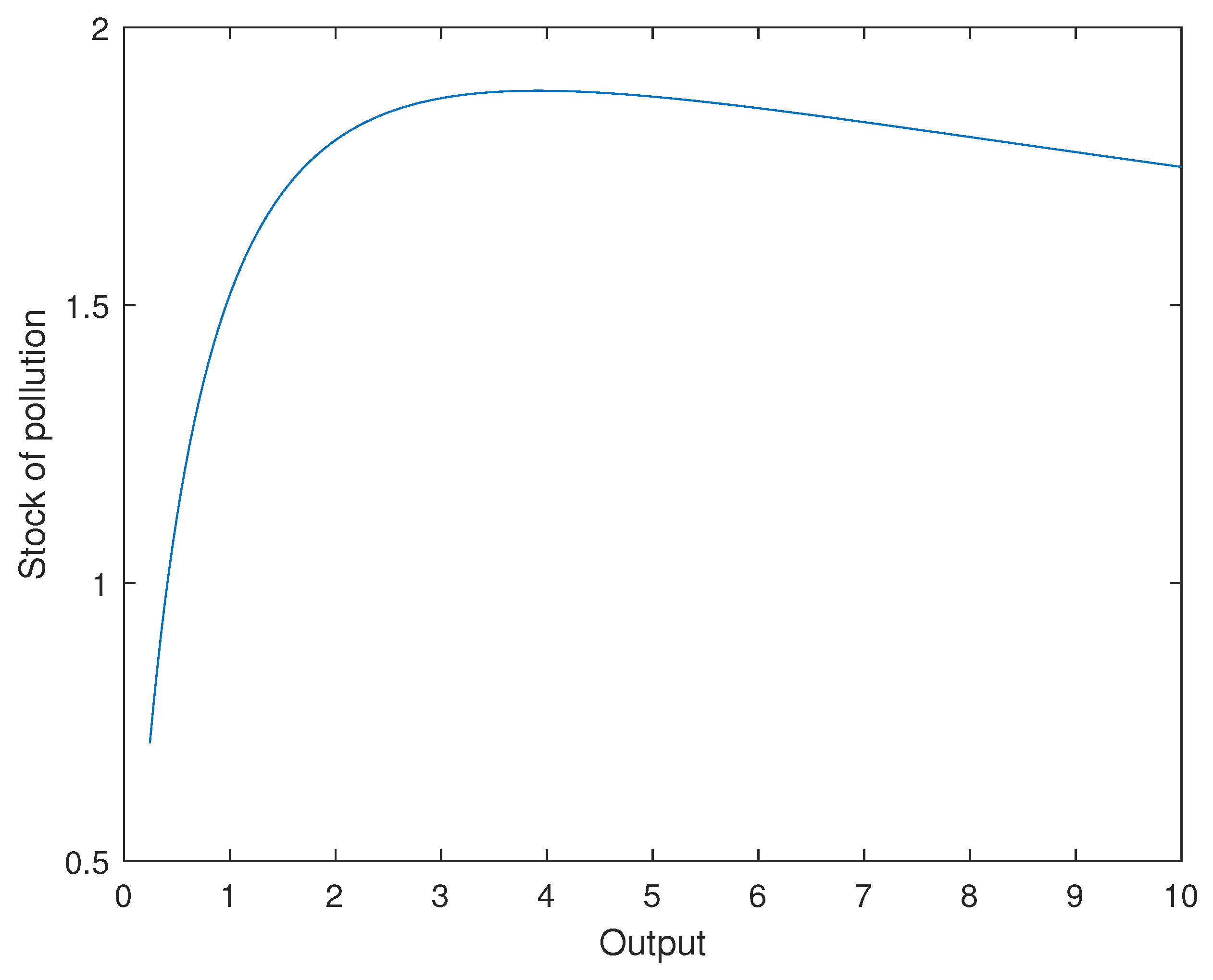
Figure 1 plots the steady-state relationship between output and the stock of pollution from the model simulation, using the benchmark calibration. We can observe that the estimated relationship between pollution and output was an inverted U-shaped curve, as stated by the EKC hypothesis. For low levels of output, the relationship between output and the stock of pollutants was positive. As we increased output, the stock of pollutants reached a maximum, and from that threshold value, the relationship between output and environmental deterioration became negative. For the EKC to exist, it was necessary that once the threshold was reached, the level of emissions was lower than the depreciation of the stock of pollution. In our framework, this was only possible if the fossil fuel consumption (the source of pollution) decreased.
The mechanisms behind this result were the following. Our model economy considered a three-factor production function, including energy, where they were complementary. This implied that to obtain more output, more energy inputs were needed. In the calibration of the model, we assumed a Cobb–Douglas production function, and hence, the elasticity of substitution among factors (physical capital, labor, and energy) was unitary. Therefore, some substitution among input factors was possible during the growth process, but the relationship between output and the quantity of energy (ruling out energy use efficiency technological change) was always positive. However, as aggregate productivity increased, energy intensity (measured as energy consumption per output unit) declined. (We investigated a CES production function where the elasticity of substitution between physical capital and energy was lower than one, but the results did not change.) Second, the model assumed, following Nordhaus [2], that the damage of emissions on productivity increased exponentially. This implied that the pollution externality cost, measured in terms of final output, increased more than proportionally as more energy was needed in the production process. This increased the relative price of “dirty” energy sources with respect to “clean” energy sources. As a consequence, as the stock of pollution increased, there was a substitution process across energy sources, where “dirty” energy sources were changed to “clean” energy sources. This substitution effect made the reduction in emissions compatible with the rise in total energy consumption. Therefore, it was the increase in the price of the fossil fuels energy source relative to the price of the renewable energy source, measured as losses in productivity, that was the underlying mechanism that explained the resulting EKC. These results were consistent with the model of Tahvonen and Salo [11], which supported the EKC hypothesis, but different from most of the existing environmental-economic models [13,15,16,28], in which the EKC did not work.
The simulated EKC produced by the model showed an interesting property. The EKC was not symmetric, as was generally assumed in the empirical literature when estimating a reduced-form equation between an environment indicator and income (level and square). Instead, the slope of the curve was different when the maximum was reached. The model simulated relationship increased rapidly during the first state of economic development, but once the stock of pollutants reached its maximum, the negative slope was very flat, indicating that the negative elasticity of pollutants to output was very small. This implied that once the stock of pollutants reached its maximum, the reduction in the stock of pollutants was a slow process as the level of output was increasing. Of course, technological progress related to the energy use efficiency or to the level of emissions per energy unit could accelerate the reduction in the stock of pollutants. Other technological advances, such as artificial Carbon dioxide Capture and Removal (CCR) technologies could increase the negative elasticity between pollution and output. However, our finding was meaningful as it demonstrated that the EKC could be produced just by neutral technological change, as an optimal reaction of the economy by changing the energy mix when the damage to productivity started to be large enough.
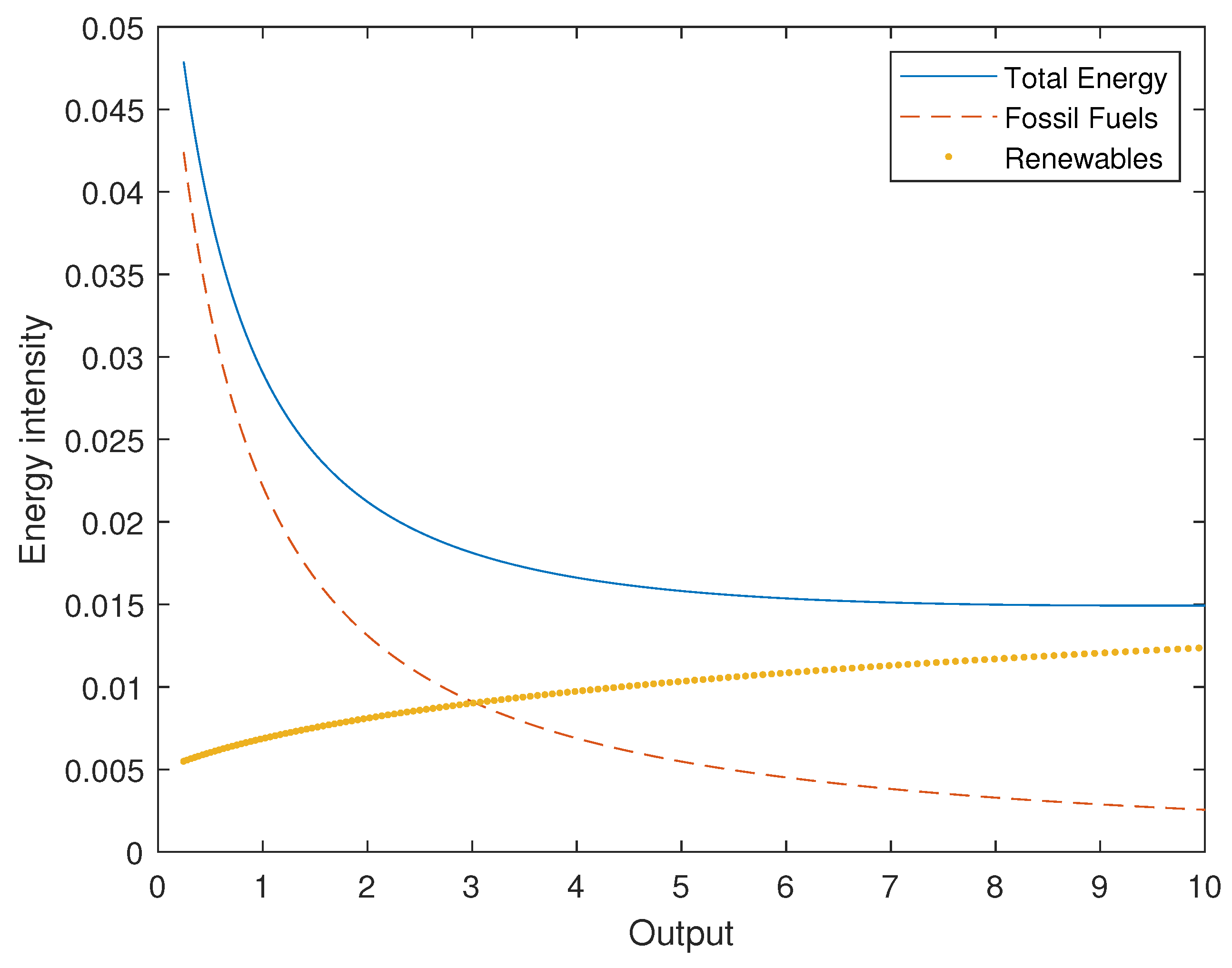
Figure 2 plots the steady-state values for energy intensity. Total energy intensity declined as output increased, a result consistent with the empirical evidence, indicating that the growth rate of output was higher than the growth rate of energy consumption, as a fraction of output growth was explained by aggregate productivity improvements. Energy intensity from the two alternative energy sources showed a different pattern. Whereas fossil fuel energy intensity reduced, renewable energy intensity increased. This result was derived from the changes in the energy mix. As output increased, fossil fuel consumption declined, whereas consumption of renewable energy increased, resulting in different changes in energy intensity depending on the energy source. However, the increase in renewable energy intensity was not problematic as this was a “clean” energy with no negative impact on the environment.
6. Sensitivity Analysis and Discussion
The structural estimation of the EKC presented above was a benchmark estimation conditional on the particular parameterization of the model, presented in Table 1. Therefore, it was necessary to carry out a sensitivity analysis to evaluate how the benchmark EKC estimation responded to changes in the parameters. Here, we carried out this sensitivity analysis for a range of values of the relevant parameters affecting the steady-state relationship between final output and the stock of pollution: the elasticity of substitution between fossil fuels and renewable energy, the elasticity of aggregate productivity with respect to the stock of pollution, and the emissions efficiency parameter.
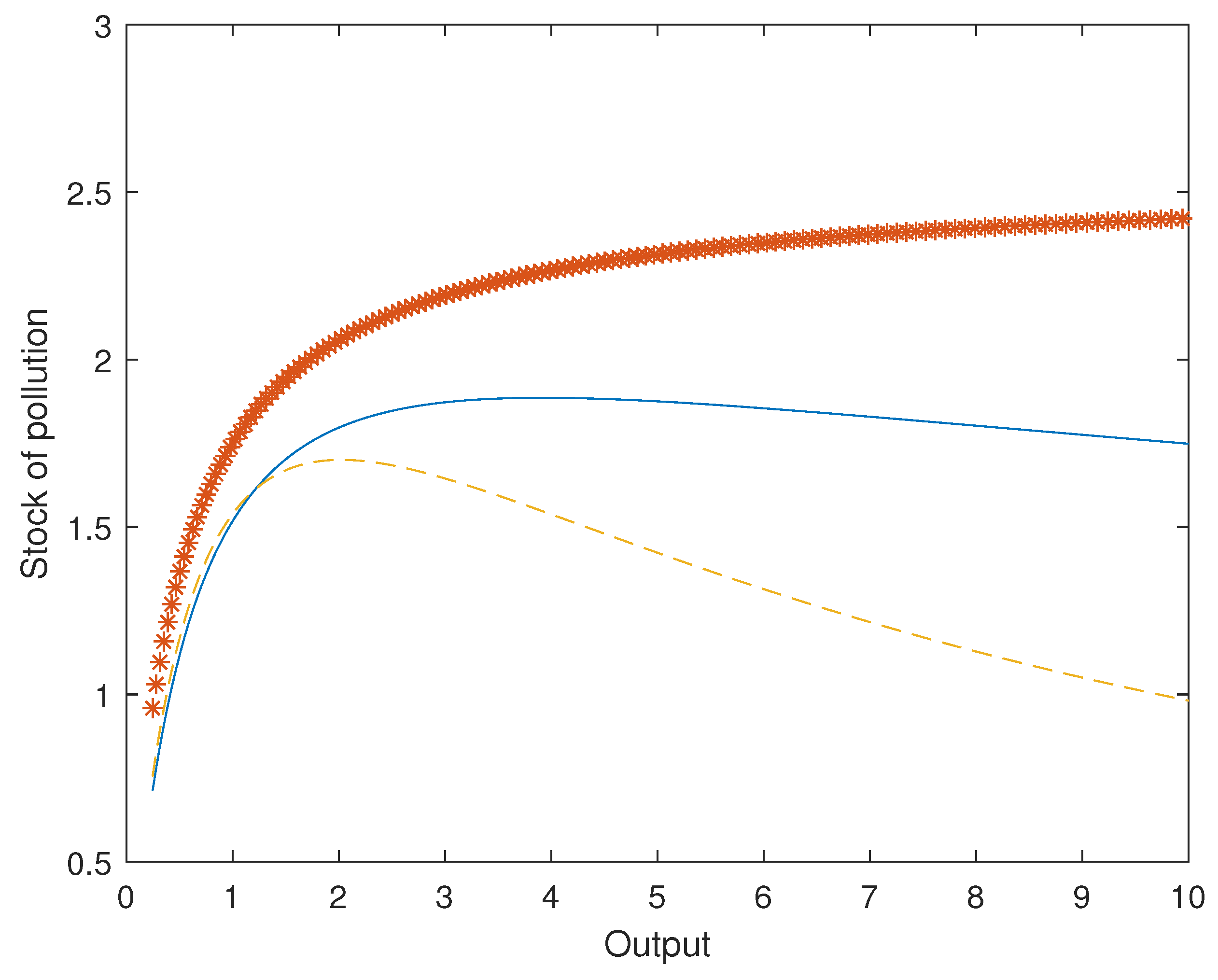
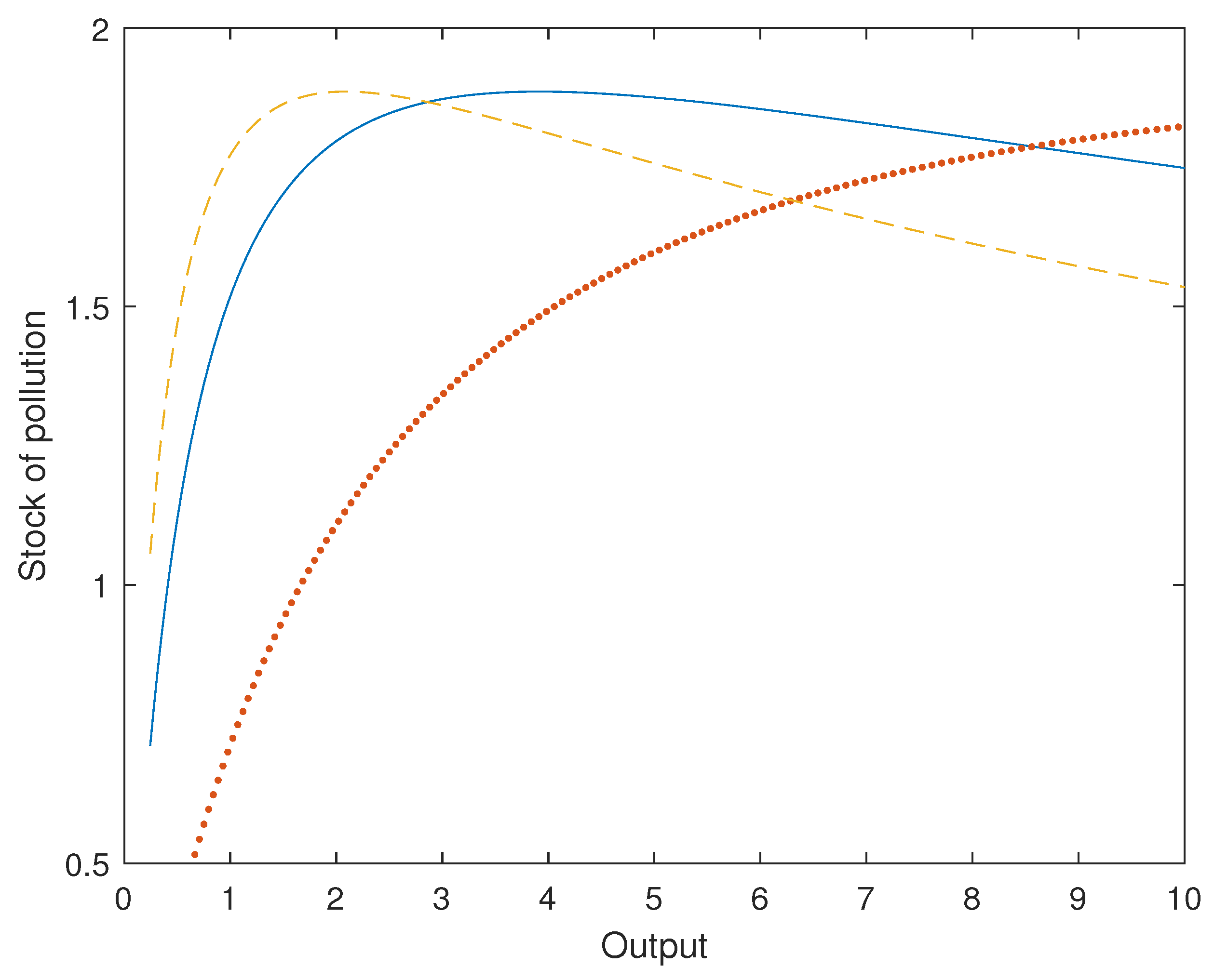
First, we studied how the output-environment deterioration relationship responded to alternative values for the elasticity of substitution between fossil fuels and renewable energy. The underlying mechanism driving the output-environment deterioration relationship was energy mix changes. Changes in the energy mix depended on the degree of substitutability between the alternative energy sources. Therefore, we expected that the value of the elasticity of substitution between fossil fuel and renewable energy was a key parameter in the estimation of the EKC. Figure 3 plots the simulated EKC depending on the value of the elasticity of substitution between fossil fuels and renewable energy. We simulated the model for three cases: a unitary elasticity of substitution, , the benchmark case where the elasticity of substitution was 1.5, and a third case where the elasticity of substitution was 2. Results showed that the steady-state output-environment relationship was very sensitive to this parameter. Furthermore, for the first case of a unitary elasticity of substitution, the EKC hypothesis was not supported, resulting in a relationship between output and the stock of pollution that was always positive, indicating that substitution of “dirty” with “clean” energy was slow compared to output growth. In this case, as output increased, the use of fossil fuel reduced, but not at a rate high enough to affect the stock of pollution negatively. The EKC appeared when the elasticity of substitution between both energy sources was above one. As the elasticity of substitution increased above one, the substitution of fossil fuel by renewable energy accelerated, resulting in a significant reduction in emissions and in the stock of pollution. Interestingly, the threshold value where the stock of pollution reached a maximum was also affected by the elasticity of substitution. The higher the elasticity of substitution between energy sources, the lower the threshold output level and the lower the maximum stock of pollution. These results were consistent with the empirical findings by Urban and Nordensvärd [36], who showed that low carbon energy transition in the Nordic countries had been fundamental for the validity of the EKC hypothesis in these economies.
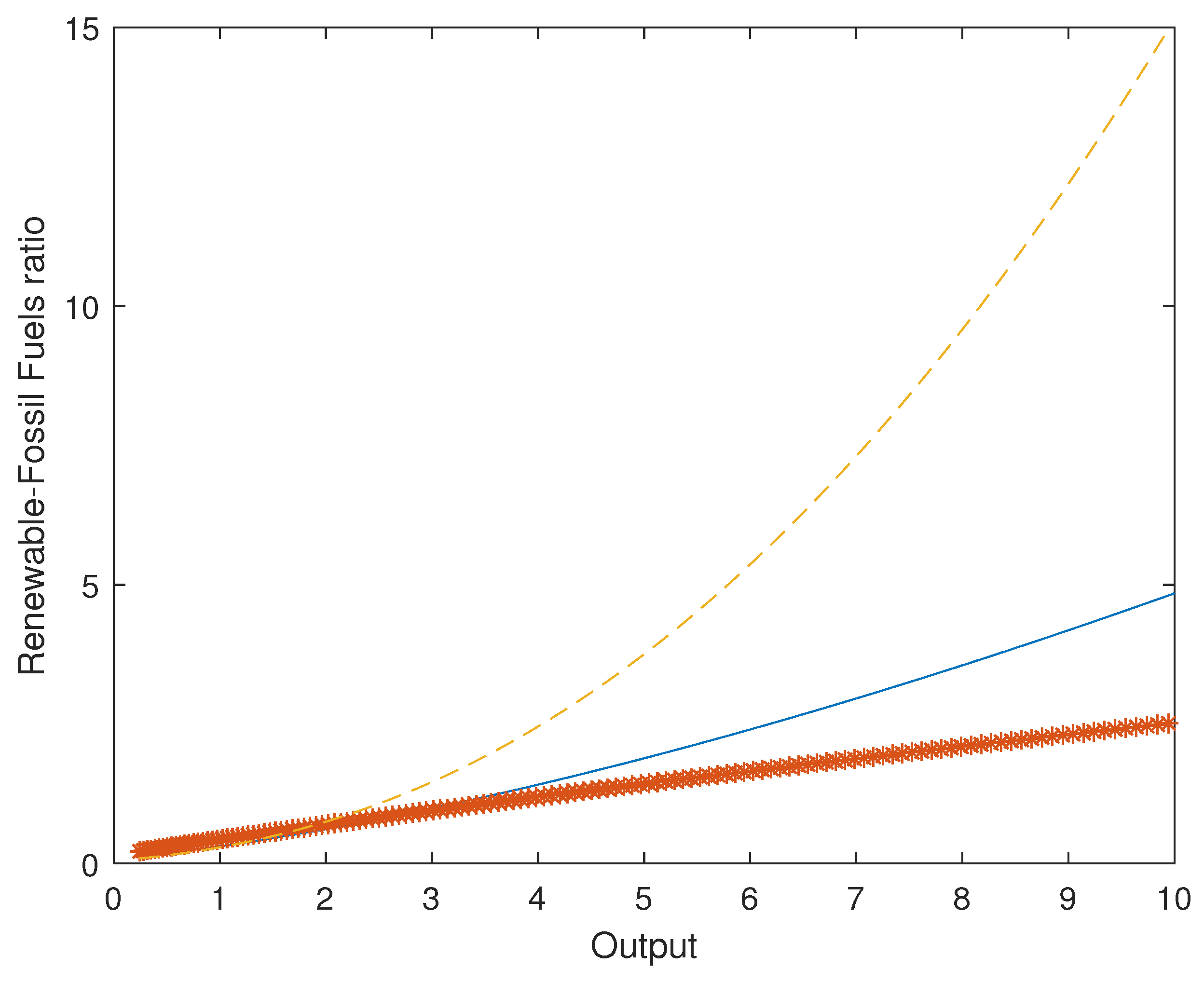
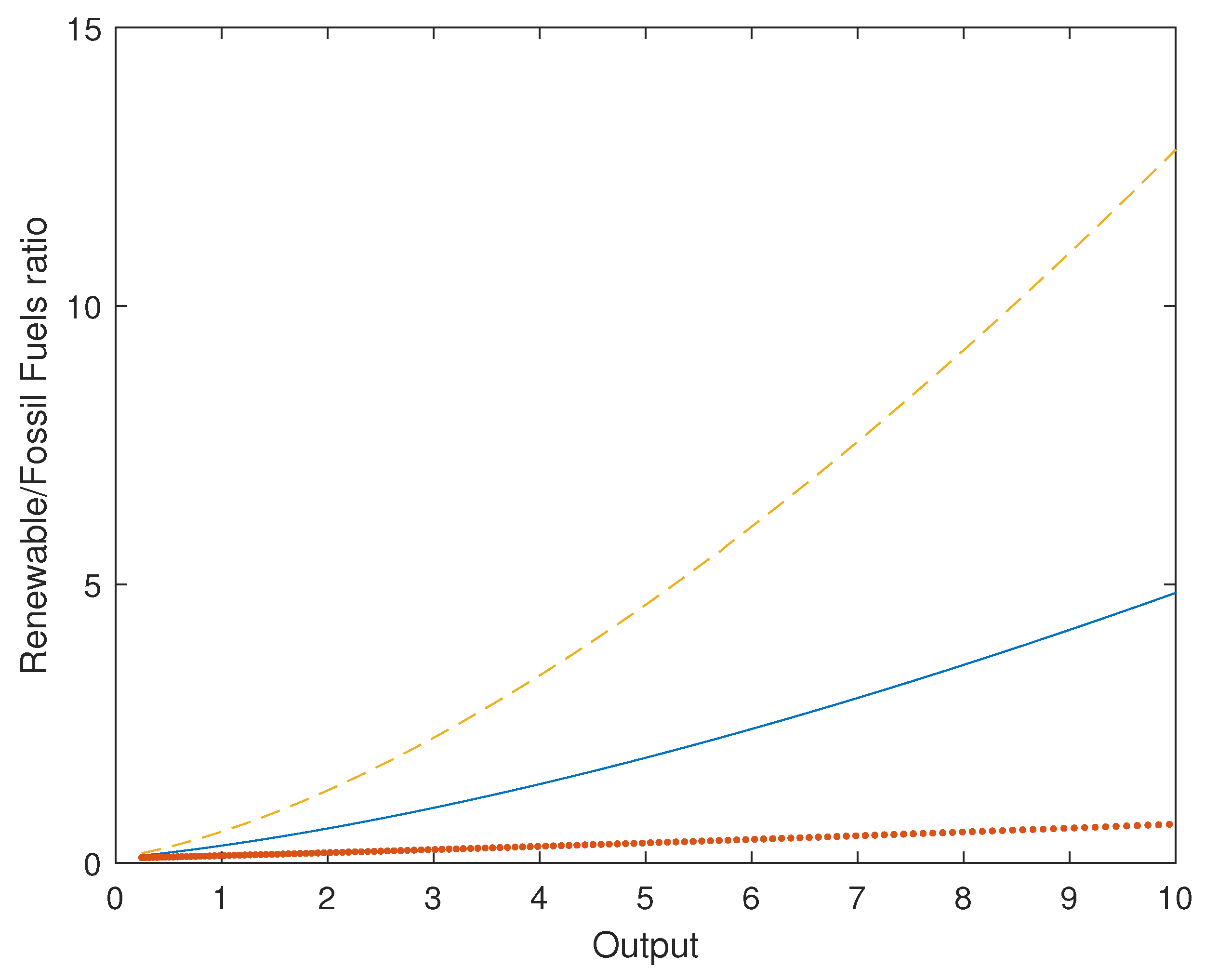
Figure 4 plots the renewable energy-to-fossil fuels ratio for the different values of the elasticity of substitution. When the elasticity of substitution was low (i.e., unitary), the renewable-fossil fuel ratio increased slowly as output increased. However, this ratio increased at an exponential rate as the elasticity of substitution was high. These results indicated that for an EKC to exist, the elasticity of substitution between “dirty” and “clean” energies must be large enough. This result highlighted the importance of energy mix policies and investment directed policies toward renewable energy as fundamental instruments to reduce environmental damages. Stern [37] carried out a meta-study of 47 studies of inter-fuel substitution, resulting in an average elasticity of 0.95. By contrast, Golosov et al. [34] used a much higher elasticity of two.
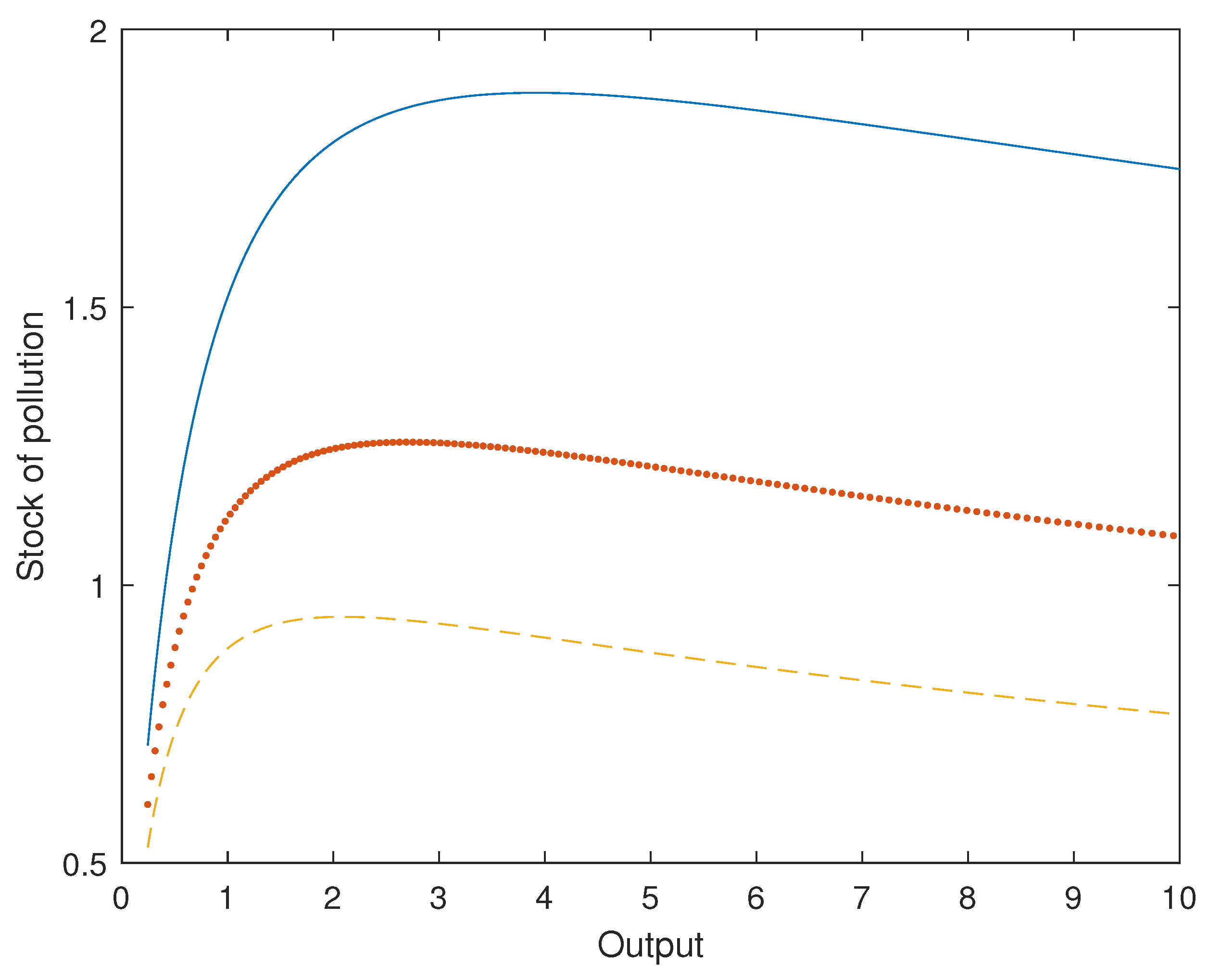
A second parameter affecting the estimation of the EKC is the pollution damage parameter to productivity. This parameter determines the negative impact of the stock of pollution on aggregate productivity. In the model, the negative impact of the stock of pollution on aggregate productivity was assumed to be an exponential function, following Özokcu and Özdemir [24]. The parameter measures the losses in aggregate productivity as a function of the stock of pollution, representing how harmful pollution is for the quality of the environment. In principle, we could expect that the lower this parameter, the better for the economy and the environment. However, we also expected that as this parameter was higher, the substitution of “dirty” energy with “clean” energy would be fostered, having a positive impact on the environment. This could be counterintuitive, as it implied that the greater the damage to the economy per unit of pollution, the better for the environment. Figure 5 plots the simulated EKC for different values of the pollution damage parameter (the benchmark case , 0.15, and 0.2). We observed that independently of the value of this parameter, an EKC was obtained. On the other hand, the maximum for the stock of pollution and the threshold output value differed depending on this parameter. As the damage parameter increased, both the threshold output value and the maximum stock of pollution declined. Furthermore, the accumulation of pollution was lower as the damage parameter increased. Therefore, paradoxically, a high damage parameter was better for the environment.
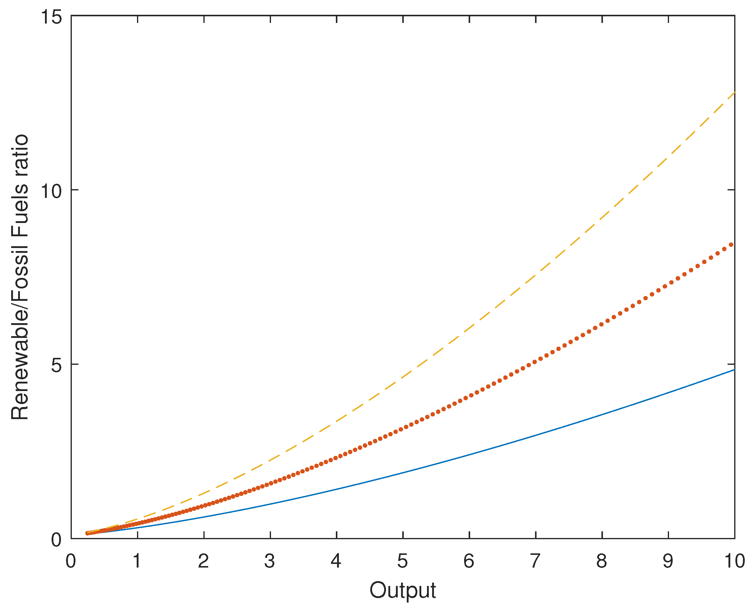
Figure 6 plots the ratio between renewable energy and fossil fuel depending on the damage parameter, which explained the EKCs in the above figure. The lower the damage parameter, the lower the substitution of “dirty” energy with “clean” energy, which explained an EKC with a very high stock of pollution. The damage parameter is key for determining the social cost of fossil fuel. A higher damage parameter increases the relative price of fossil fuel with respect to renewable energy, which incentives the substitution of the former with the latter energy source. This reduces emissions for any income level, reducing the pollution accumulation process.
Finally, we studied the sensitivity of the EKC to the parameter representing the level of emissions per fossil fuel unit. This is an emissions efficiency parameter that can be regulated by environmental policies establishing limits to emissions. Figure 7 and Figure 8 plot the EKC and the renewable fossil fuels ratio for different values of the parameter reflecting the level of emissions per unit of fossil fuel consumed. We found that increasing emission efficiency had a positive effect on the environment for low levels of income, but not for high incomes, as this parameter did not change the accumulation process of pollution, but its timing. Indeed, as we increased the level of emissions efficiency, the negative slope side of the EKC disappeared, resulting in a positive relationship between environmental deterioration and output, for the range of income values in the simulations. Damage to the environment per unit of fossil fuel consumed was lower when emissions efficiency was higher, but this simply delayed the accumulation of pollution.
The most important result was that the maximum stock of pollution was always the same independently of the emissions parameter, but the threshold output value differed. As emissions efficiency increased, the threshold output value also increased. However, the timing changed. When emissions efficiency was high, the accumulation of pollutants was low as output increased. This was because emissions per unit of fossil fuel energy were also very low and little substitution between fossil fuel and renewable energy was produced. However, when emissions efficiency was lower, this accelerated the accumulation of pollutants, as more emissions per unit of fossil fuel were generated. However, this process also accelerated the substitution of “dirty” with “clean” energy, reducing the output for which the stock of pollution reached a maximum.
The variability of the emission parameter across time and countries could explain why the empirical literature had obtained mixing results (see, for instance, [26,27,28,29]) depending on the countries and period samples. The value of this parameter was determined by the combination of different fossil fuels (coal, oil, and gas), where carbon emissions generated by each source were different. Therefore, for the empirical estimation of the EKC was necessary not only to control for the energy mix between non-renewable and renewable energy sources, but also the fraction of each type of fossil fuel.
From the above results, we could derive an important environmental policy recommendation: emissions efficiency policies did not contribute to preserving environmental quality in the long-run, although they were effective in the short-run. This was a counterintuitive result, as authorities have made considerable efforts in implementing policies for increasing emissions efficiency. Examples of these policies are limits to emissions and the promotion of catalytic inverter technologies. These policies are designed to mitigate damage to the environment. However, our analysis revealed that these policies might be ineffective in the long-run. Whereas these policies were effective at reducing environmental damage in the short-run, they disincentivized the substitution of “dirty” energy with “clean” energy, increasing the accumulation of pollution in the long-run. In other words, the accumulation process of pollution did not change as a function of emissions efficiency; this only delayed the process. This is an important issue to be taken into account when designing and implementing emissions reduction policies.
Overall, the results presented in this paper were consistent with the literature that studies the relationship among output, renewable and non-renewable energy consumption, and the environment, and they offered an explanation of the missing results obtained by the empirical literature estimating the ECK hypothesis. A number of empirical works [38,39,40,41,42,43,44] have found a direct impact between renewable energy consumption and the presence of EKC, using different econometric techniques and sample countries. Dogan and Seker [38] studied the role of renewable and non-renewable energy consumption on carbon emissions for the European Union. They showed that the split of energy consumption between renewable and non-renewable energy sources had dramatic consequences on the estimation of the EKC. Their results indicated that renewable energy mitigated carbon emissions and supported the EKC hypothesis, an empirical result consistent with the theoretical analysis in this paper in which the EKC hypothesis depended on the energy transition from non-renewable to renewable energy sources. Jebli et al. [39] and Erdogan et al. [44] carried out a similar analysis for a panel of 25 OECD countries, the two arriving at similar results. Dogan and Ozturk [40] studied the case of the U.S. and found that the ECK hypothesis was not valid for this country, but also estimated that increases in renewable energy consumption mitigated environmental degradation, whereas increases in non-renewable energy consumption contributed to carbon emissions. These results not only applied to developed countries, but similar results were obtained in the case of developing countries, as shown by Danish et al. [41] and Gill et al. [42]. Le et al. [43] considered a sample of 102 countries, including both developed and developing economies, and found that the use of non-renewable energy consumption significantly increased emissions across different income groups of countries, but that the use of renewable energy sources mitigated carbon emissions in developed countries, but not in developing economies. Finally, the energy mix of a particular economy also depends on the sectorial structure, a link that could explain the results found by Le et al. [43]. Lin et al. [45] and Dogan and Iglesi-Lotz [46] highlighted the implications of the economic structure for the presence of an EKC, as the importance of the industry is directly related to the energy mix and, hence, the level of emissions.
7. Conclusions and Policy Implications
Long-run sustainable economic growth and environmental protection are dynamically linked by the existence of an intertemporal constraint resulting from the negative impact of the stock of pollutants on production. A key element of the relationship between economic growth and the environment is the so-called Environmental Kuznets Curve (EKC) hypothesis, which establishes the existence of a U-shaped relationship between income and environmental quality. For low levels of income, economic growth leads to environmental deterioration, whereas for high levels of income, economic growth reduces environmental damages.
The literature has focused on the role of alternative environmental policies to mitigate environmental damage, including abatement policies, taxes, etc., or directed technical change as a key driving force to reduce pollutant emissions. In this paper, we argued that the most effective path to mitigate environmental damage was the introduction of changes in the energy mix to be redirected to the use of cleaner energy sources. To study the relationship between output, the energy mix, and the environment, this paper developed an environmental-DGE model where productivity was negatively affected by the stock of pollutants. The model used a three-factor production function: capital, labor, and energy. Two energy sources were considered: fossil fuels energy and renewable energy. Emissions were generated by the use of fossil fuel in the energy production activity. Model simulations supported the EKC hypothesis. As income increased, initially, the level of emissions increased, reaching a maximum, from which, output reduced the level of emissions. The explanation of this result was the following. As output increased, the pollution externality cost also increased, reducing productivity. This made the use of “dirty” energy more expensive relative to renewable “clean” energy. The increase in the fossil fuels/renewable energy relative price, measured in units of final output, provoked a substitution of “dirty” energy with “clean” energy, resulting in a decrease in the level of emissions. However, simulations of the model revealed that while the positive slope part of the EKC was much steeper, the negative slope part of the EKC was estimated to be very flat. This result meant that once the economy reached the maximum environmental deterioration level, the output-environmental deterioration negative elasticity was very small and little gain in environmental quality was produced as income further increased. This negative elasticity depended on the effects of environmental deterioration on productivity.
Finally, the paper investigated the sensitivity of the estimated EKC to changes in the key parameters determining the steady-state relationship between output and the stock of pollution. First, the EKC hypothesis was only met when the elasticity of substitution between fossil fuel and renewable energy was sufficiently high (higher than one). If the elasticity of substitution between both energy sources was unitary, the EKC did not hold. As the elasticity of substitution increased, the maximum level of pollution declined, and a greater decrease in the stock of pollution was obtained as output increased. Second, the higher the elasticity of productivity to the stock of pollution, the lower the optimal stock of pollution as a function of output. This was a counterintuitive result as worse (more damage to the economy) was better (for the environment). Finally, we studied the impact of emissions efficiency and found that it did not affect the accumulation of pollution, but affected its timing. As emissions efficiency increased, pollution accumulated slowly for any level of income. From this result, we obtained an important policy implication: emissions efficiency policies did not contribute to solving the problem of pollution and only contributed to delaying the problem.
Funding
This research was funded by the Spanish Ministry of Science, Innovation and Universities Grant Number ECO-2016-76818-C3-2-P, Research Project UMA18-FEDERJA-145, and Universidad de Málaga.
Acknowledgments
I thank three anonymous referees for very useful comments and suggestions on an earlier version of this article. Part of this project was carried out while I was visiting the Department of Economics at the Universidad Autónoma de Madrid, the hospitality of which I gratefully acknowledge.
Conflicts of Interest
The author declares no conflict of interest.
Abbreviations
The following abbreviations are used in this manuscript:
| EKC | Environmental Kuznets Curve |
| GPD | Gross Domestic Product |
| DGE | Dynamic General Equilibrium |
| TFP | Total Factor Productivity |
| BLS | Bureau of Labor Statistics |
| EIA | U.S. Energy Information Administration |
| Output | |
| Stock of physical capital | |
| Labor | |
| Energy | |
| Consumption | |
| Investment | |
| Fossil fuel | |
| Renewable energy | |
| Price of fossil fuel | |
| Price of renewable energy | |
| Carbon emissions | |
| Stock of pollution | |
| Total factor productivity | |
| Discount factor | |
| Aversion risk parameter | |
| Willingness to work | |
| The Frisch elasticity | |
| Output-capital elasticity | |
| Output-energy elasticity | |
| Depreciation rate of physical capital | |
| Weight of fossil fuel | |
| Energy substitution parameter | |
| Emissions parameter | |
| Decay rate of the stock of pollutants | |
| Pollution damage parameter |
Appendix A
The central planner maximization problem can be defined using the following Lagrangian auxiliary function:
The first order conditions for the consumer maximization problem are:
From first order conditions, we obtain the following values for the Lagrangian multipliers:
Substituting in first order conditions for the consumer maximization problem, we obtain the equilibrium condition for the working hours:
The optimal consumption path is given by:
The optimal stock of pollution is defined by:
References
- World Commission on Environment and Development. Our Common Future; United Nations: New York, NY, USA, 1987. [Google Scholar]
- Nordhaus, W. A Question of Balance: Weighing the Options on Global Warming Policies; Yale University Press: New Haven, CT, USA, 2008. [Google Scholar]
- Barbier, E.B. The Concept of Sustainable Economic Development. Environ. Conserv. 1987, 14, 101–110. [Google Scholar] [CrossRef]
- Grossman, G.M.; Krueger, G.M. Environmental Impacts of a North American Free Trade Agreement; National Bureau of Economic Research: Cambridge, MA, USA, 1991. [Google Scholar]
- Grossman, G.M.; Krueger, G.M. Economic Growth and the Environment. Q. J. Econ. 1995, 110, 353–377. [Google Scholar] [CrossRef] [Green Version]
- Kuznets, S. Economic Growth and Income Inequality. Am. Econ. Rev. 1955, 45, 1–8. [Google Scholar]
- John, A.; Pecchenino, R. An Overlapping Generations Model of Growth and the Environment. Econ. J. 1994, 104, 1393–1410. [Google Scholar] [CrossRef]
- López, R. The Environment as a Factor of Production: The Effects of Economic Growth and Trade Liberalization. J. Environ. Econ. Manag. 1994, 27, 163–184. [Google Scholar] [CrossRef]
- Jones, L.E.; Manuelli, R.E. Growth and the Effects of Inflation. J. Econ. Dyn. Control. 1995, 19, 1405–1428. [Google Scholar] [CrossRef] [Green Version]
- Stokey, N. Are There Limits to Growth? Int. Econ. Rev. 1998, 39, 1–31. [Google Scholar] [CrossRef]
- Tahvonen, O.; Salo, S. Economic growth and transitions between renewable and nonrenewable energy sources. Eur. Econ. Rev. 2001, 45, 1379–1398. [Google Scholar] [CrossRef]
- Gill, A.R.; Viswanathan, K.K.; Hassan, S. The Environmental Kuznets Curve (EKC) and the environmental problem of the day. Renew. Sustain. Energy Rev. 2018, 81, 1636–1642. [Google Scholar] [CrossRef]
- Heutel, G. How should environmental policy respond to business cycles? Optimal policy under persistent productivity shocks. Rev. Econ. Dyn. 2012, 15, 244–264. [Google Scholar] [CrossRef] [Green Version]
- Fischer, C.; Springborn, M. Emissions targets and the real business cycle: Intensity targets versus caps or taxes. J. Environ. Econ. Manag. 2011, 62, 352–366. [Google Scholar] [CrossRef]
- Angelopoulos, K.; Economides, G.; Philippopoulos, A. What is the best environmental policy? Taxes, permits and rules under economic and environmental uncertainty. In DEOS Working Papers 1014; Athens University of Economics and Business: Athens, Greece, 2010. [Google Scholar]
- Angelopoulos, K.; Economides, G.; Philippopoulos, A. First- and second-best allocations under economic and environmental uncertainty. Int. Tax Public Financ. 2013, 20, 360–380. [Google Scholar] [CrossRef]
- Annicchiarico, B.; Di Dio, F. Environmental policy and macroeconomic dynamics in a new Keynesian model. J. Environ. Econ. Manag. 2015, 69, 1–21. [Google Scholar] [CrossRef] [Green Version]
- Shafik, N.; Bandyopadhyay, S. Economic Growth and Environmental Quality: Time Series and Cross-Country Evidence; World Bank Working Paper WPS 904; World Bank: Washington, DC, USA, 1992. [Google Scholar]
- Holtz-Eakin, D.; Selden, T. Stoking the fires? CO2 emissions and economic growth. J. Public Econ. 1995, 57, 85–101. [Google Scholar] [CrossRef] [Green Version]
- Selden, T.; Song, D. Environmental Quality and Development: Is There a Kuznets Curve for Air Pollution Emissions? J. Environ. Econ. Manag. 1994, 27, 147–162. [Google Scholar] [CrossRef]
- Panayotou, T. Empirical Test and Policy Analysis of Environmental Degradation at Different Stages of Economic Development; Working Paper, ILO; International Labour Organization: Geneva, Switzerland, 1993. [Google Scholar]
- Shafik, N. Economic Development and Environmental Quality: An Econometric Analysis. Oxf. Econ. Pap. 1994, 46, 757–773. [Google Scholar] [CrossRef]
- Panayotou, T. Demystifying the environmental Kuznets curve: Turning a black box into a policy tool. Environ. Dev. Econ. 1997, 2, 465–484. [Google Scholar] [CrossRef] [Green Version]
- Özokcu, S.; Özdemir, Ö. Economic Growth, energy and environmental Kuznets curve. Renew. Sustain. Energy Rev. 2017, 72, 639–647. [Google Scholar] [CrossRef]
- Dogan, E.; Seker, F. The influence of real output, renewable and non-renewable energy, trade and financial development on carbon emission in the top renewable energy countries. Renew. Sustain. Energy Rev. 2016, 60, 1074–1085. [Google Scholar] [CrossRef]
- Stern, D.I. Progress on the environmental Kuznets curve? Environ. Dev. Econ. 1998, 3, 173–196. [Google Scholar] [CrossRef]
- Dinda, S. Environmental Kuznets Curve Hypothesis: A Survey. Ecol Econ 2004, 49, 431–455. [Google Scholar] [CrossRef] [Green Version]
- Kaika, D.; Zervas, E. The Environmental Kuznets Curve (EKC) theory-Part A: Concept, causes and the CO2 emissions case. Energy Policy 2013, 62, 1392–1402. [Google Scholar] [CrossRef]
- Kaika, D.; Zervas, E. The Environmental Kuznets Curve (EKC) theory-Part B: Critical issues. Energy Policy 2013, 62, 1403–1411. [Google Scholar] [CrossRef]
- Andreoni, J.; Levinson, A. The simple analytics of the environmental Kuznets curve. J. Public Econ. 2001, 80, 269–286. [Google Scholar] [CrossRef] [Green Version]
- Stern, D.I. The Environmental Kuznets Curve; Rensselaer Polytechnic Institute: Troy, NY, USA, 2003. [Google Scholar]
- Brock, W.A.; Taylor, M.S. The green Solow model. J. Econ. Growth 2010, 15, 127–153. [Google Scholar] [CrossRef]
- Kijima, M.; Nishide, K.; Ohyama, A. Economic models for the environmental Kuznets curve: A survey. J. Econ. Dyn. Control 2010, 34, 1187–1201. [Google Scholar] [CrossRef]
- Golosov, M.; Hassler, J.; Krusell, P.; Tsyvinski, A. Optimal taxes on fossil fuels in general equilibrium. Econometrica 2014, 82, 41–88. [Google Scholar]
- Heathcote, J.; Storesletten, K.; Violante, G.L. The macroeconomic implications of rising wage inequality in the United States. J. Polit. Econ. 2010, 118, 681–722. [Google Scholar] [CrossRef] [Green Version]
- Urban, F.; Nordensvärd, J. Low Carbon Energy Transitions in the Nordic Countries: Evidence from the Environmental Kuznets Curve. Energies 2018, 11, 2209. [Google Scholar] [CrossRef] [Green Version]
- Stern, D.I. Interfuel substitution: A meta-analysis. J. Econ. Surv. 2012, 26, 307–331. [Google Scholar] [CrossRef] [Green Version]
- Dogan, E.; Seker, F. Determinants of CO2 emissions in the European Union: The role of renewable and non-renewable energy. Renew. Energy 2016, 94, 429–439. [Google Scholar] [CrossRef]
- Jebli, M.B.; Youssef, S.B.; Oztur, I. Testing environmental Kuznets curve hypothesis: The role of renewable and non-renewable energy consumption and trade in OECD countries. Ecol. Indic. 2016, 60, 824–831. [Google Scholar] [CrossRef]
- Dogan, E.; Ozturk, I. The influence of renewable and non-renewable energy consumption and real income on CO2 emissions in the USA: Evidence from structural break tests. Environ. Sci. Pollut. Res. 2017, 24, 10846–10854. [Google Scholar] [CrossRef]
- Zhang, B.; Wang, B.; Wang, Z. Role of renewable energy and non-renewable energy consumption on EKC: Evidence from Pakistan. J. Clean. Prod. 2017, 156, 855–864. [Google Scholar]
- Gill, A.R.; Viswanathan, K.K.; Hassan, S. A test of environmental Kuznets curve (EKC) for carbon emission and potential of renewable energy to reduce green house gases (GHG) in Malaysia. Environ. Dev. Sustain. 2018, 20, 1103–1114. [Google Scholar] [CrossRef]
- Le, T.H.; Chang, Y.; Park, D. Renewable and Nonrenewable Energy Consumption, Economic Growth, and Emissions: International Evidence. Energy J. 2020, 41, 73–92. [Google Scholar] [CrossRef]
- Erdogan, S.; Okumus, I.; Guzel, A.E. Revisiting the Environmental Kuznets Curve hypothesis in OECD countries: The role of renewable, non-renewable energy, and oil prices. Environ. Sci. Pollut. Res. 2020. [Google Scholar] [CrossRef]
- Lin, B.; Omoju, O.E.; Nwakeze, N.M.; Okonkwo, J.U.; Megbowon, E.T. Is the environmental Kuznets curve hypothesis a sound basis for environmental policy in Africa? J. Clean. Prod. 2016, 133, 712–724. [Google Scholar] [CrossRef]
- Dogan, E.; Inglesi-Lotz, R. The impact of economic structure to the environmental Kuznets curve (EKC) hypothesis: Evidence from European countries. Environ. Sci. Pollut. Res. 2020, 27, 12717–12724. [Google Scholar] [CrossRef]
Sample Availability: MatLab codes are available from the author. |
Figure 1.
The environmental Kuznets curve: relationship between output and stock of pollution.

Figure 2.
Energy intensity as a function of output.

Figure 3.
EKC. Change in the elasticity of substitution between fossil fuels and renewable energies. Solid line: benchmark case, . Dashed line: . Starred line: .
Figure 3.
EKC. Change in the elasticity of substitution between fossil fuels and renewable energies. Solid line: benchmark case, . Dashed line: . Starred line: .

Figure 4.
Ratio of renewable-to-fossil fuels. Change in the elasticity of substitution between fossil fuels and renewable energies. Solid line: benchmark case, . Dashed line: . Starred line: .
Figure 4.
Ratio of renewable-to-fossil fuels. Change in the elasticity of substitution between fossil fuels and renewable energies. Solid line: benchmark case, . Dashed line: . Starred line: .

Figure 5.
EKC. Change in the pollution damage parameter. Solid line: benchmark case, . Starred line: . Dashed line: .
Figure 5.
EKC. Change in the pollution damage parameter. Solid line: benchmark case, . Starred line: . Dashed line: .

Figure 6.
Renewable-to-fossil fuel ratio. Change in the pollution damage parameter. Solid line: benchmark case, . Starred line: . Dashed line: .
Figure 6.
Renewable-to-fossil fuel ratio. Change in the pollution damage parameter. Solid line: benchmark case, . Starred line: . Dashed line: .

Figure 7.
EKC. Change in the emissions parameter. Solid line: benchmark case, . Starred line: . Dashed line: .
Figure 7.
EKC. Change in the emissions parameter. Solid line: benchmark case, . Starred line: . Dashed line: .

Figure 8.
Fossil fuel-to-renewable ratio. Change in the emissions parameter. Solid line: benchmark case, . Starred line: . Dashed line: .
Figure 8.
Fossil fuel-to-renewable ratio. Change in the emissions parameter. Solid line: benchmark case, . Starred line: . Dashed line: .


Table 1.
Calibration of the parameters.
| Parameter | Definition | Value | |
|---|---|---|---|
| Preferences | Discount factor | 0.975 | |
| Risk aversion | 1.2 | ||
| Labor weight | 15.60 | ||
| Frisch elasticity parameter | 0.72 | ||
| Technology | Output-capital elasticity | 0.2518 | |
| Output-energy elasticity | 0.0982 | ||
| Physical capital depreciation rate | 0.07 | ||
| Energy | Weight of fossil fuels | 0.73 | |
| Energy substitution | 1.50 | ||
| Environment | Emissions parameter | 0.1 | |
| Pollutant stock decay rate | 0.012 | ||
| Pollution damage parameter | 0.0875 |
© 2020 by the author. Licensee MDPI, Basel, Switzerland. This article is an open access article distributed under the terms and conditions of the Creative Commons Attribution (CC BY) license (http://creativecommons.org/licenses/by/4.0/).
Share and Cite
MDPI and ACS Style
Bongers, A. The Environmental Kuznets Curve and the Energy Mix: A Structural Estimation. Energies 2020, 13, 2641. https://doi.org/10.3390/en13102641
AMA Style
Bongers A. The Environmental Kuznets Curve and the Energy Mix: A Structural Estimation. Energies. 2020; 13(10):2641. https://doi.org/10.3390/en13102641
Chicago/Turabian StyleBongers, Anelí. 2020. "The Environmental Kuznets Curve and the Energy Mix: A Structural Estimation" Energies 13, no. 10: 2641. https://doi.org/10.3390/en13102641
Note that from the first issue of 2016, this journal uses article numbers instead of page numbers. See further details here.