A Fuzzy-SOM Method for Fraud Detection in Power Distribution Networks with High Penetration of Roof-Top Grid-Connected PV


1
Faculty of New Sciences and Technologies, University of Tehran, Tehran 1439957131, Iran
2
School of Electrical and Computer Engineering, University of Tehran, Tehran 1417414418, Iran
*
Author to whom correspondence should be addressed.
Energies 2020, 13(5), 1287; https://doi.org/10.3390/en13051287
Submission received: 2 February 2020
/
Revised: 3 March 2020
/
Accepted: 4 March 2020
/
Published: 10 March 2020
(This article belongs to the Special Issue Integration of Large-Scale Renewable Energy Sources into the Low-Inertia Power Grid)
Abstract
:This study proposes a fuzzy self-organized neural networks (SOM) model for detecting fraud by domestic customers, the major cause of non-technical losses in power distribution networks. Using a bottom-up approach, normal behavior patterns of household loads with and without photovoltaic (PV) sources are determined as normal behavior. Customers suspected of energy theft are distinguished by calculating the anomaly index of each subscriber. The bottom-up method used is validated using measurement data of a real network. The performance of the algorithm in detecting fraud in old electromagnetic meters is evaluated and verified. Types of energy theft methods are introduced in smart meters. The proposed algorithm is tested and evaluated to detect fraud in smart meters also.
1. Introduction
Power grids fall into three main sectors of production, transmission and distribution. A large portion of the power grid losses belongs to distribution networks due to their expansiveness, speed of development and inappropriate operation. In 2018, 10.79% of the electricity delivered to Iran’s national grid was lost in distribution. That is equivalent to a stunning amount of 32 billion kWh [1]. Generally, electrical energy losses are the portion of electricity that is injected into the transmission and distribution grid but is not paid for by end-users. In other words, part of the electricity injected into the transmission and distribution grid, which does not generate any revenue for the electricity providers, is called loss of electricity. Electricity losses consist of two main components, namely “technical losses” and “non-technical losses”. Technical losses occur due to the current passing through the inherent characteristic of electrical resistance of the conductors of the grid. These types of losses are found in transmission and distribution lines, transformers and metering systems. Non-technical losses originate from off-system activities and occur in various forms, including electricity theft, non-payment by subscribers, and errors in recording and calculating energy costs. An important issue facing the problem of losses in electricity distribution networks is the serious challenge of unclear share of technical and non-technical losses in the networks. Calculated technical losses are not reliable because of insufficient information, poor quality of equipment, poor installation quality and low operational quality. Introduction of small-scale generators into the grid, and especially small domestic solar units, as well as wind mini-generators, micro-hydro generators, etc. has increased the complexity of assessing electrical energy losses, especially in the non-technical sector. The conventional rule of detecting non-technical losses in power distribution companies includes field visiting and testing customer meters. The aforementioned methods result in less detection of those subscribers who disrupt their meters at certain times but for the whole metering period. The non-technical losses imposed on the power grid thus account for a significant share of total non-technical losses. In addition, the high number of customers and the need to test all network meters make these methods very costly. In practice, in many cases the high cost of testing equipment, the cost of manpower and the cost of transporting swallows a large portion of the revenue from non-technical loss recovery.
Numerous studies have so far provided useful solutions to detect such fraud. A method for detecting fraud by high-voltage customers is presented in [2,3]. The methods presented in these studies are based on artificial intelligence and data mining and have achieved successful results. Another interesting research work is that of Monedero et al. [4]. The proposed method based on artificial neural networks was used in the Spanish Seville power grid, and the remarkable result was a 50% improvement in the detection of non-technical casualties compared to previous methods. In general, methods for detecting non-technical losses and unauthorized use of the power grid can be divided into three categories: theoretical methods, hardware methods and data analysis methods [5]. Among these, data-analysis-based methods have the highest share, which in practice are preferred over other methods because of the high cost of meter testing or installation of consumption monitoring hardware. Numerous proposed and tested methods have had significant results in monitoring and reducing technical losses, but technological changes such as smart grids techniques and technologies [6], digital meter technology, and the development of domestic energy generation using on-grid rooftop photovoltaic (PV) panels have created complexities in non-technical loss-detection models. Various articles have focused on the detection of non-technical losses and unauthorized use of the network in smart networks [6,7,8,9], but the issue of non-technical losses in networks with large numbers of grid-connected small scale generations has been considered in few research works. The effect of such resources on non-technical losses of distribution grids, has received less attention in the literature. Expanding the use of almost no-cost solar/mini-wind/micro-hydro power (apart from initial investment costs) will generally encourage a minimal use of the costly network energy, but the problem arises when there are similarities between the behavior of subscribers suspected of manipulating meters and subscribers using these small resources. This similarity of consumption behavior makes it difficult to distinguish these two types of subscribers using the methods presented in previous research. This study focuses on rooftop grid-connected solar resources, where the model may be extended to mini-wind and micro-hydro generation using the relevant resource models.
There are also some other small-scale resource technologies such as small parabolic solar collectors which are mostly used for heating and cooking, hence are not included in the study.
The basic goals of this study can be summarized as follows:
- Accelerating detection and control of non-technical losses of distribution networks.
- Controlling the cost of detecting non-technical losses in power distribution companies.
- Providing an efficient model for consumption management.
- Modeling the effect of renewable resource development on customers’ load behavior.
Modeling the non-technical losses of distribution networks in this study is fully consistent with a variety of conventional energy theft methods. The comprehensive model presented is applicable to a wide range of distribution networks, both traditional and modern smart distribution networks, which has received little research attention.
Customers’ energy consumption is measured using modern smart meters in the Iranian power distribution network, but there are still significant numbers of electromagnetic or old digital meters in the network. Due to the differing data resolution available in traditional meters and smart meters, the detection method of non-technical losses of these two types of subscribers is different in some stages. The method presented in this study is based on data-mining models. Since some subscribers who have successfully passed the meter test process may also have attempted energy theft, the consumption data of the verified meters alone cannot provide a precise pattern of customer consumption behavior. We use a bottom-up approach to determine the electrical energy consumption pattern. Electrical load profiles are generated for customers with and without rooftop photovoltaic resources.
The proposed bottom-up model simulates the random behavior of the customers and, thus, the load profile may be different from one customer to another. The effect of rooftop PV on load profile is then. This study considers photovoltaic systems equipped with maximum power point tracking (MPPT). A method based on self-organized neural networks (SOM), is proposed to detect suspected subscribers to fraud and consumption anomalies. The model is then evaluated in a real sample network.
2. Modeling Domestic Load Profile
We need to know the behavior of loads, and in particular, domestic customers in this study. Some studies of power distribution networks such as master planning, loss reduction studies and protection coordination studies use cumulative models of load behavior. A common method of analyzing load behavior is to measure the simultaneous power consumption of a number of customers of a particular category (e.g., domestic, commercial, industrial, etc.) and extend it to other customers of the same category using coincidence factors [10]. The factor decreases as the number of subscribers increases. Examples of coincidence curves are given in different references such as in [11]. The peak demand obtained from these methods is used to design the network and coordinate protection relays, but for applications such as load management and energy theft analysis, a higher resolution of power consumption data is required. The cumulative load behavior curve is the sum of individual customers’ load profiles, and the load profile of each individual customer is the sum of the load behavior of its electrical appliances. The methods used to aggregate the behavior of electrical appliances to reach the customer’s load behavior are called “bottom-up” methods [12,13,14,15]. The bottom-up approach is recognized as one of the most widely used methods that enables the study of consumer behavioral patterns and the effects of load response programs [16]. These can be achieved by examining the behavioral pattern for using home appliances [17] or by using the data of energy bills together with specific questionnaires [18]. The latter method is based on statistical data that can be very accurate in analyzing buildings energy demand [18]. Some studies have used such accurate information on residents and home appliances to model electricity consumption [19,20,21] while others have used methods to extract random models that reduce the need for detailed and accurate statistical information [22,23,24,25,26]. A bottom-up approach has been used to model the energy consumption of a home by considering the level of activity of consumers (either when residents are at home or when they are not) and their behavior pattern in [27]. Another model has been developed for studying electricity and hot water consumption based on consumption time data in [20], where a good accuracy of results compared to actual and measured values is demonstrated. Important features of the bottom-up methods are categorized in [28], the most important of which are:
- It is simple and easy to implement.
- Macroeconomic and social factors can also be included in the model.
- It is very suitable for determining the energy consumption and related parameters.
- It is always capable of developing, computing and newer studies.
- It does not require very detailed information and can be conducted using billing data and questionnaires.
Therefore, the bottom-up approach is a good way to extract the energy consumption curve as it involves the behavior patterns of residents and the use of different appliances [27]. Due to the necessity of knowing the consumption behavior of each individual household, the bottom-up method is used in this study to extract the load profile.
2.1. Typical Domestic Load Profile
Household consumption in cold and hot seasons has a completely different behavior pattern in most areas of Iran. The main reason is the different types of heating and cooling systems. The increase in the share of vapor compression cooling in recent years has led to a significant jump in the country’s peak load during the warm season. In order to better understand the pattern of load behavior, we take a closer look at the load consumed by home subscribers.
Reference [10] classifies home electrical appliances into four categories: brown goods, white goods, minor appliances, and lighting systems. Relatively low consumption electronic equipment such as communication equipment, desktops, scanners, CD/DVD players, TVs, modems etc. belong to the category of brown goods. Basic household necessities are called white appliances. These include kitchenware, laundry and heating and cooling appliances. Minor appliances are the type of electrical equipment that are typically found in any home and are usually portable. Some of these minor appliances include: electric kettle, toaster, juicer, coffee maker, ironing, fan, vacuum cleaner, sewing machine, mobile phones, home digital cameras, radios, mp3 players, tablets, hair dryer, shaver, etc.
Various factors affect the load profile of household subscribers, the most important of which are:
- Temperature in terms of maximum summer temperature and minimum winter temperature.
- Yearly average temperature.
- Economic factors such as the price of all types of energy resources such as electricity, gas, etc., the price of household electrical appliances, the per capita income of the household, and the economic situation of the community.
- Demographic factors such as the number of households and population growth over a given period.
- Welfare level and infrastructure level of houses.
The modeling performed in this study and the measurement results along with the simulation results confirm the significant effect of summer daytime temperature on the load behavior curve.
2.2. Mathematical Modeling of Load Profile
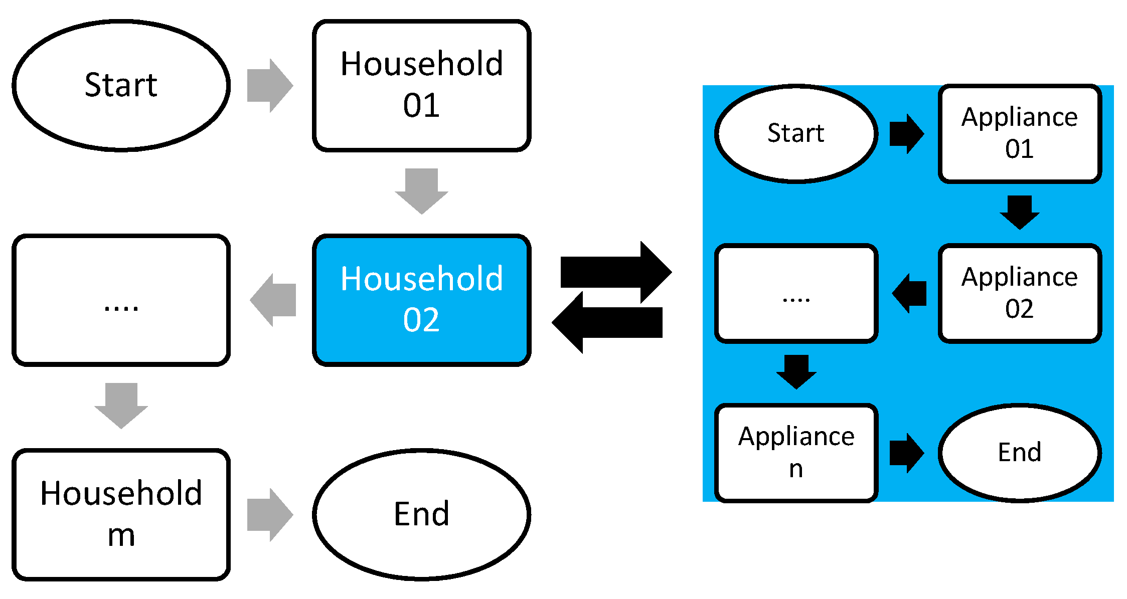
A prominent feature of the bottom-up model is that it can be used to analyze the load behavior of each individual subscriber. Figure 1 illustrates the logic used for modeling. The daily load curve is actually created by repeating two loops. In the first loop, after choosing the type of household, a load curve will be created for each of the equipment in the house. This procedure is repeated in the second loop for all the equipment and the cumulative consumption curve is added to the previous curves to obtain the final household load curve. The appliance list varies from house to house, so a coefficient is defined as the level of saturation that indicates the likelihood of a particular home being equipped with a particular appliance (). In fact, for a large number of homes, this coefficient gives the frequency of a particular home appliance. For example, a saturation level of 0.93 for an appliance in 100 residential homes means that there are 93 units of that special equipment in the 100 homes [13].
Assuming that the equipment list and associated saturation range are known, a mathematical model is needed to construct the energy consumption curve. The basic idea is that if a particular appliance is switched on, the power consumption will be added from the time step of switching on to the whole house until the equipment operation cycle is completed and the equipment is switched off. The daily consumption curve will be calculated from the sum of each individual consumption curve when this process is repeated for all appliances. Depending on the customer’s consumption pattern, a specific appliance can be switched on at any time of the day at various times. This part is actually one of the most important parts of modeling. In this study, a start probability function () is introduced representing the probability of the appliance turning on at each time step. Any electrical appliance has the highest chance of being turned on at certain times of the day. A clear example of this is the lighting lamps that are most likely to be lit in the early hours of the night, but that does not mean that they do not start at other times. For the mathematical definition of this problem, for each appliance, the probability distribution function is defined whose maximum value or values correspond to peak hours of probability of start, and the starting probability at other times follows a normal distribution pattern. takes a value between zero and one. When the appliance is off, the search for the next start begins based on . This is done by generating a random number of probability distributions related to it. When the appliance turns on and completes its duty cycle, the search for the next switch-on time begins. The probability function can be calculated using the following equation [13]:
where is related to three variables, indicates the type of the proposed appliance, is the calculation time step, is the daily time in hours, and is the saturation level of appliance A as previously described. is the probability factor that specifies the activity level of any appliance at any time of the day. The larger the amount, the higher the probability of the appliance being turned on, and vice versa. is the frequency of turning the appliance on, which indicates the average number of times a particular appliance is used per day. is a scaling factor that scales probabilities on the basis of .
Equation (1) applies to all appliances. When an appliance is switched on, its rated power added to the customers’ load profile during the operating cycle, and then the equipment is switched off to begin the search for the next switch on. Standby power of equipment is also considered in this study. For example, refrigerators and TVs consume some power even when they are off, which is included in calculations.
3. Grid-Connected Photovoltaic Source Behavior
Small grid connected PV resources have resulted in a significant behavioral change in the load pattern by contributing to supplying part of the customer’s demand and also providing part of the grid’s required power from their surplus. This has made it necessary to consider the impact of these resources in analyzing the customer’s behavior. In this study, the effect of the performance of small photovoltaic sources on the load profile of households is investigated using mathematical modeling and computer simulation.
There are various approaches to exploiting solar generation [29]. One of the most common approaches is to generate solar energy through MPPT and to exploit the maximum solar radiation power available. When solar power is operated as MPPT, there will be no freedom to participate in frequency control, because there is no capacity to increase production in this case, however, for the small producers in this study, the main objective is to provide the power consumption and utilize the maximum capacity of the installed system. Therefore, this study investigates a photovoltaic system operated under an MPPT strategy in grid-connected mode and the performance of the proposed system in tracking maximum output power under different sunlight conditions and finally its effect on the load profile of home subscribers is considered.
3.1. Modeling of Solar Panels
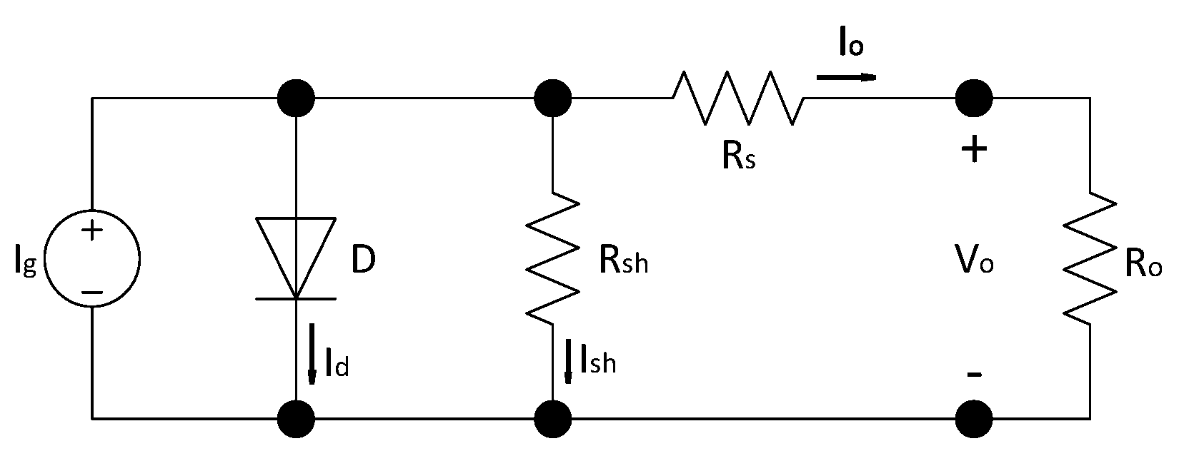
The PV module is a non-linear device that can be considered as a current source as shown in Figure 2 [30,31,32]. Regardless of the internal series resistors, the common current-voltage (I-V) equations of a solar module can be expressed as in Equation (2);
where is the output current of the PV module, is the number of cells in parallel, is the current generated by solar radiation, is the reverse saturation current, is charge of an electron, is the output voltage of PV module, is the ideality factor of the diode, is the Boltzmann’s constant and is the current due to intrinsic shunt resistance of the PV module.
The saturation current of the solar module varies with temperature fluctuations as formulated in Equation (3):
where is the saturation current at reference temperature (), is the band-gap energy, is the short-circuit current temperature coefficient, is the short-circuit current of PV module, is the solar insolation, and is temperature of the PV module in K.
The current through the shunt resistance is calculated as follows:
where Is the number of cells in series, and is the internal shunt resistance of the PV module.
3.2. Maximum Power Point Tracking (MPPT) Modeling
Several algorithms have been proposed for maximum power point tracking. These algorithms can be divided into three general categories [33,34]:
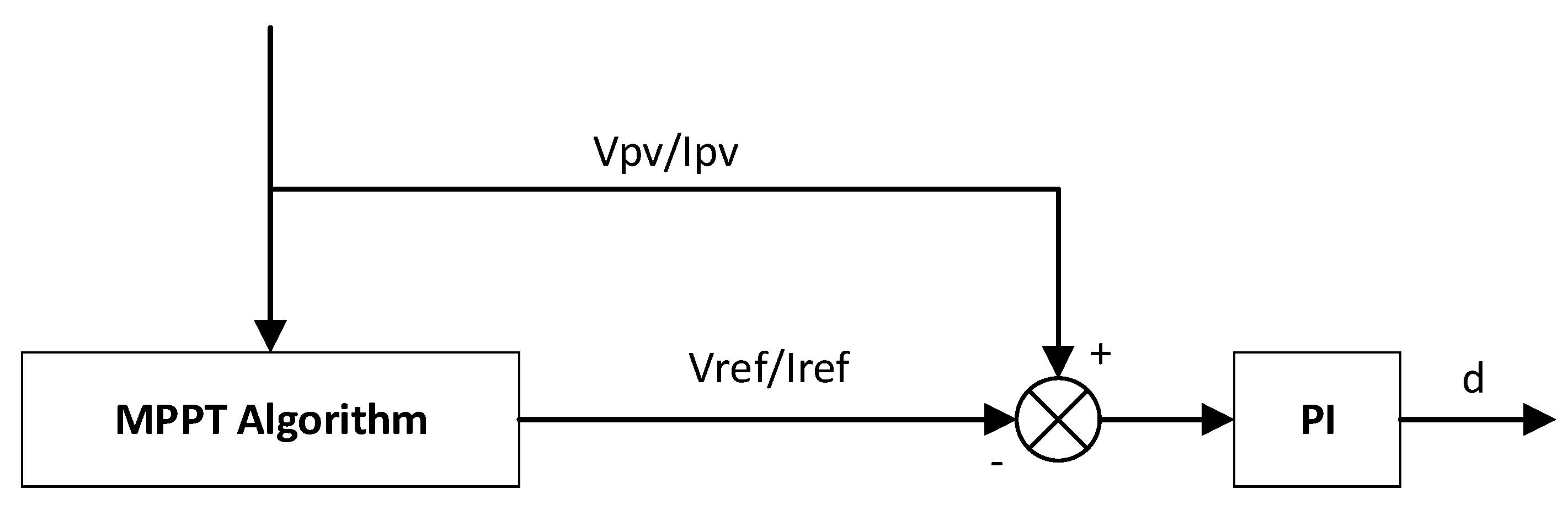
Any of the mentioned algorithms could be adapted for the purpose of this research due to the flexibility of ANN-based model used. The incremental conductance method [38,39] is used to model the maximum power point tracking in this study. The dP/dV must be equal to zero at the maximum power point [44], so:
At any given moment, the MPPT checks the zero-sum requirement of dI/dV and I/V. If the resultant is not zero, the proportional-integral (PI) controller considers the value of the product as error and minimizes it. The value at the output of the PI controller is the amount of change required in the duty cycle. This value is added to the current duty cycle value. For better convergence, the initial value of duty cycle has been set to 0.75 by trial and error. The concept of the proposed controller is shown in Figure 3.
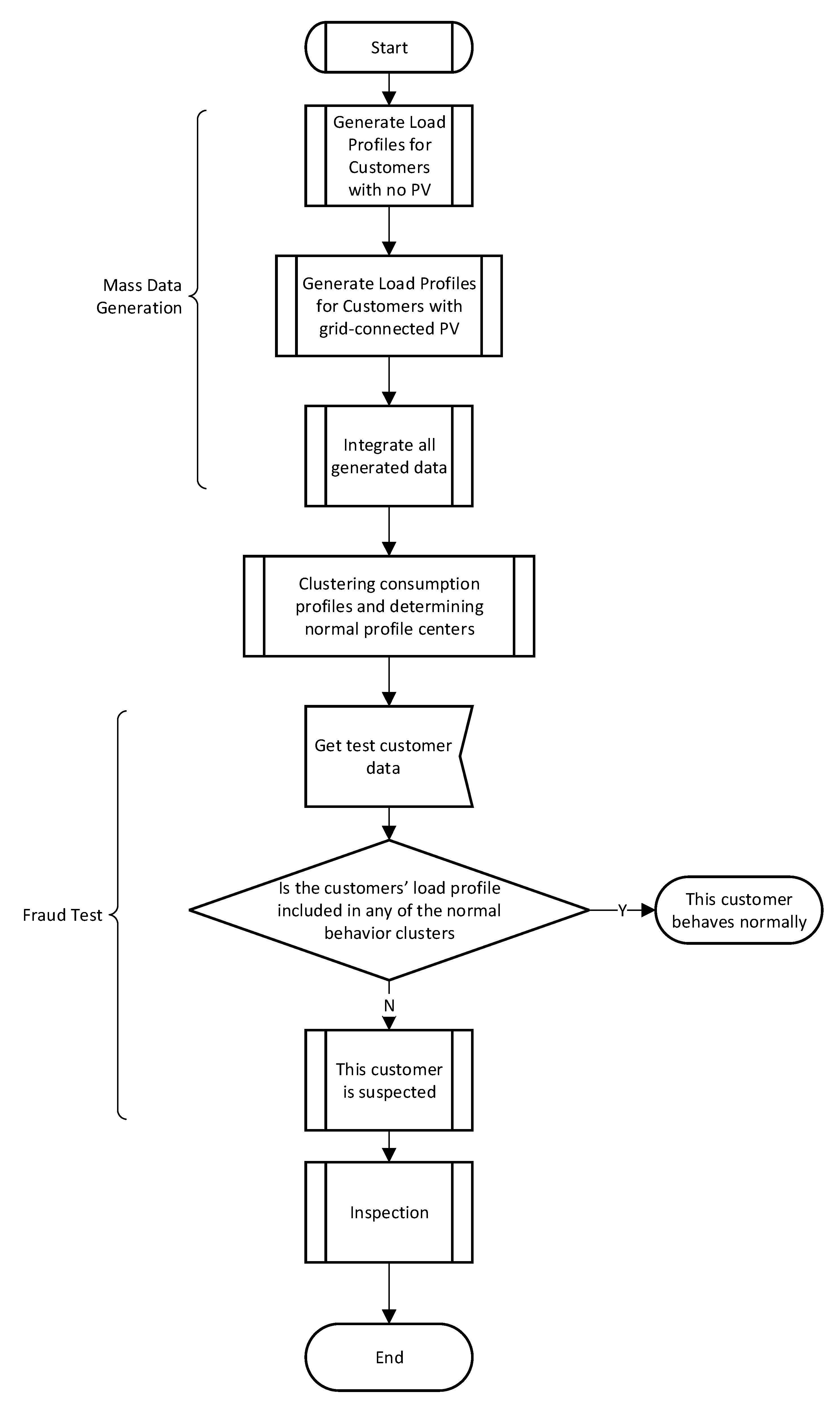
4. Data Mining Methods for Fraud Detection
Detection of anomalies is done using the famous knowledge discovery model. These models are widely used in data-mining research [2,45,46,47]. Given the similarity of energy consumption behavior in small areas with relatively homogeneous distribution and living standards, the use of non-supervised knowledge discovery methods allows data clustering. The SOM method is used for clustering and then detecting anomalies in subscriber consumption profile in this study. Anomalies in the load profile can be the result of a common fraud or a failure in the metering system, which in any case is the non-monetization of the relevant shared energy consumption for distribution companies, equivalent to non-technical losses.
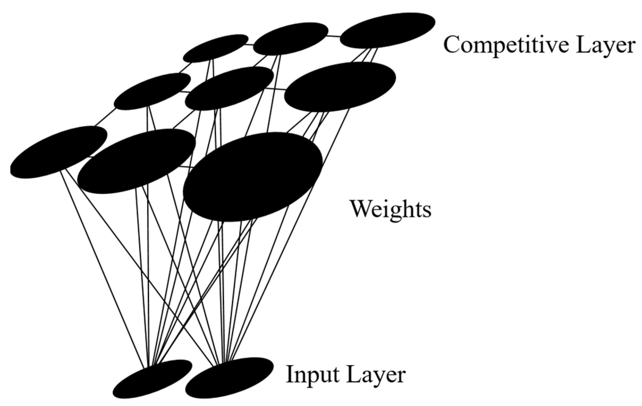
The SOM network uses competitive learning to train and is developed based on specific characteristics of the human brain. The cells in the human brain are organized in different areas so that in different sensory areas they are presented with meaningful computational maps. Self-organized networks are structurally divided into several categories in which we used the Kohonen network in this study. The SOM is an unsupervised neural network composed of neural neurons in a regular, low-dimensional grid structure. Each neuron has an n-dimensional weight vector where n is the dimension of the input vectors. Weight vectors (synapses) attach the input layer to the output layer. This is called the output layer, map or competitive layer. The neurons are connected by a neighborhood function (as shown in Figure 4). Each input vector, by most similarity, activates a neuron in the output layer called the winning cell. The similarity is usually measured by the Euclidean distance between two vectors [48].
where is the ith input vector of the neural network, is the the weight vector which connects the ith input to the jth output, and is the sum of the Euclidean distance between input sample and its associated weight vector to output j called a map unit.
The most important difference between the SOM training algorithm and other vector quantization algorithms is that in addition to the highest matching unit weight (the winner neuron), the weights of the neighboring cells of the winning cell are also updated. Close-up observations in the input space activate two close-up units in the map. The training phase continues until the weight vectors reach steady state and no longer change:
where is the updated weight vector between input cell i and output cell j, is the previous weight vector between input vector and weight vector to output neuron j, and is the neighboring function.
After the training phase, i.e., in the mapping phase, it will be possible to automatically classify each input data vector. In the training phase, auxiliary tags such as shared zip code (specifying geographical area and living standard), main fuse capacity of meter, type of meter (digital or analog), tariff type and meter reading period (time tag) are used. The anomaly detection algorithm in electrical energy consumption is illustrated in Figure 5. The procedure for detecting abnormalities in a customer’s behavior is such that a mass-normal behavioral dataset is generated by simulation. This data is used as the input data of a SOM network for neural network training, and after clustering the bulk data, the centers of each cluster are considered as the normal behavior center. Among the consumption profiles located in each cluster, profiles whose elements have the maximum Euclidean distance to the center of the respective cluster are considered as normal boundary load profiles and customers located outside this boundary are classified as suspected substrates. The Euclidean distance of the suspected subscribers to the anomaly is normalized based on 9 and the normalized distance of any suspected subscriber from the nearest center of the cluster is defined as the “anomaly index”.
The procedure for detecting anomalies in customers’ behavior is such that a mass data of normal behavior is generated by simulation. This data is used as the input data of a SOM network for neural network training, and after clustering the bulk data, the centers of each cluster are considered as the normal behavior centers. The load curve of each customer lies at a specified distance from the centers of the clusters. The distance of each load curve from the center of the corresponding cluster is calculated using Equation (10):
where is the distance of the ith load curve from the center of the jth cluster. t is the time, is the load of the ith customer at time t, is the load of the center of the jth cluster at time t, and is the number of clusters. The membership function of each load curve in any cluster is calculated as below:
where is the membership of any customers to normal behavior.
5. Case Study
5.1. Simulation of the Load Profile of Household Customers
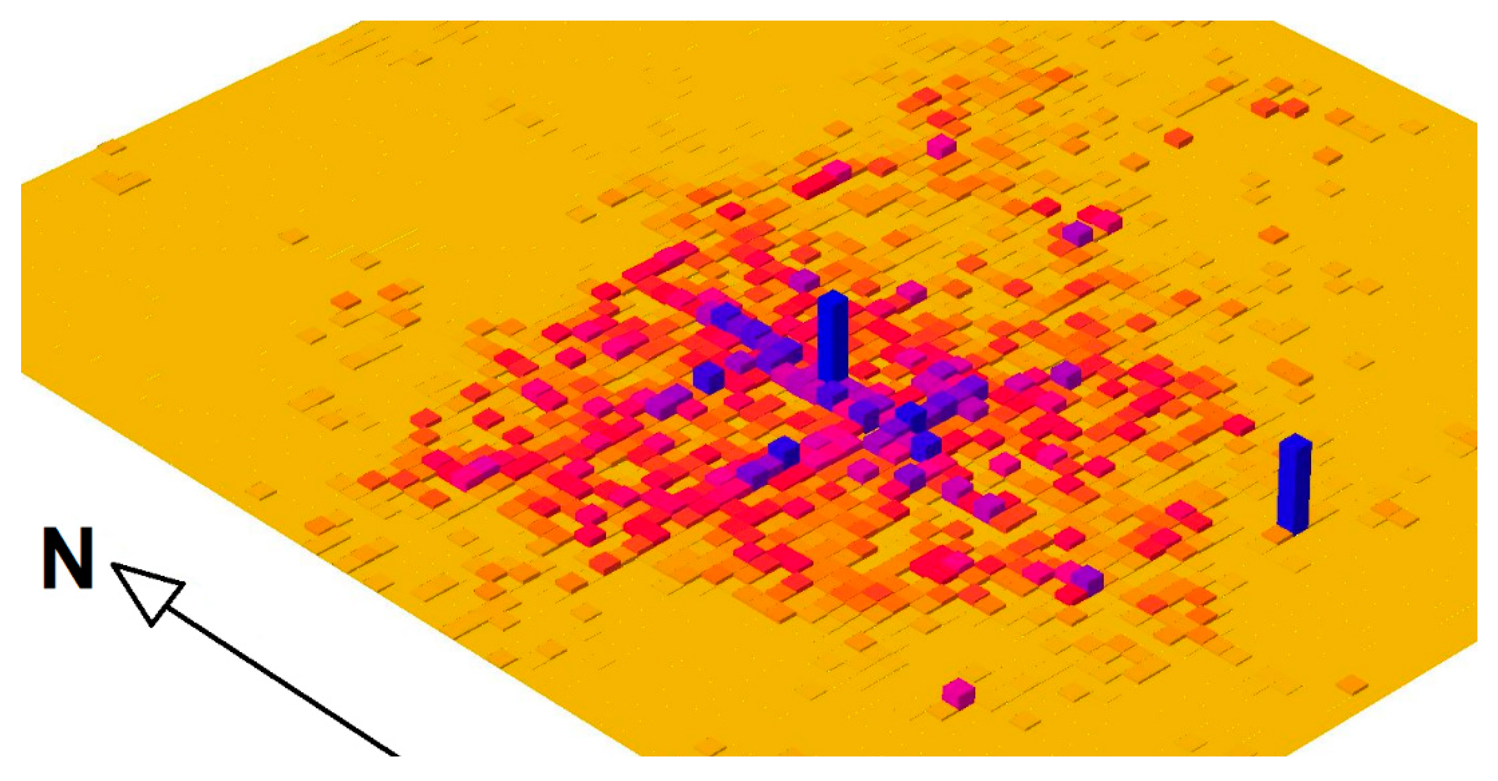
Characteristics of electrical consumer appliances of a total of 76 residential houses were collected using a questionnaire in Golgouah, Mazandaran, Iran. All meters of these customers were tested and evaluated prior to the measurements. All of these subscribers are powered by a 20/0.4 kV-160 kVA pole-mounted substation. A TDL104 data logger was used to measure these customers’ consumption and extract the load behavior curve. In 30 min time intervals, the information of the instantaneous active power, the instantaneous reactive power, the instantaneous voltage and the average consumed energy were measured for a total of 82 customers [49]. The results obtained in the measurement are used to validate the proposed model. In order to obtain homogeneous and analytic information, it has been attempted to perform measurements on feeders with similar welfare levels. For this purpose, a three-dimensional map of the load density of domestic loads was implemented in the geographic information system (GIS) for the city of Galougah (Figure 6) [50]. The specifications of the feeder measured are given in Table 1.
Based on the data obtained from the questionnaires, home appliance brands of the Iranian market and the energy label class of appliances, the list of home appliances used was extracted as described in Table 2. The pattern used in this section is adapted from [13]. Equation (1) is applied to any of the electrical energy-consuming appliances. At the beginning of each computational step, a random number between 0 and 1 is generated and compared with . If is greater than the random number generated, the consumer switches on and remains on until . After that, the process of checking the condition for the next switch-on begins again. If the appliance also has a certain power consumption in standby mode, its standby power is added to the entire power consumption curve as a constant. This holds true for loads such as televisions. The value of is the average time period each appliance stays on [13].
The consumed energy by each home during the one-month period can be calculated using Equation (12). Equation (12) gives the required values for verifying the proposed model in electric power distribution networks with no smart energy metering systems.
where is the standby power of each appliance (W), is the nominal power of each appliance (W), is the number of appliances in each home, and is the the average time period that each appliance stays on.
Mathematical simulation is performed using MATLAB. The simulation is done for one day and is extended to thirty days. The behavior of loads such as refrigerators and cooling systems largely depends on the behavior of homeowners, but the modeling of this problem will be very complex. For simplification, the average single-cycle behavior of these types of equipment is used to simulate. Simulations and measurements are related to the warm season of the year.
Subscriber well-being is another issue that has a profound effect on subscriber behavior. This study uses data from subscribers with approximately equal welfare levels. Baseline information of Table 2 is used for the simulations. This data arrangement, adapted from [13], has been modified to fit the home appliance available in the Iranian market [51]. The table also includes a column called saturation level, which is the ratio of the number of household appliances of each type to the total number of dwellings under study. The switch-on likelihood of each of the appliances listed in Table 2 varies at different times of the day. For example, it is clear that the switch-on probability of the cooling system are highest in the hot hours of the day. Also, lighting loads are more likely to happen at night. Values less than 1 for the start frequency in Table 2 mean that the appliance is switched on once in a few days. For example, the value of 0.22 for the washing machine indicates that this equipment is mostly turned on once every four to five days and does not function daily. is the probability of each equipment turning on at any given time step. In this study, unlike similar studies, the start-on probability distribution function of each device is used instead of using a constant start-on program [52] or using a specified value as the start-up probability of each device on every hour [13,19]. The starting probability distribution function of each appliance is assumed to be normal around the maximum possible start hours. Figure 7 shows the start-on probability density of each of the equipment listed in Table 2. Equipment such as air coolers are more likely to start during hot hours, but in the case of refrigerators, no hours predominate over other hours, as seen.
The simulation using the proposed model generates the behavioral curve of each electrical appliance. The total load curve of each house is obtained by integrating the load behavior curves of the electrical equipment inside it. Figure 8 shows the load behavior of several household customers with different load behavior types. The horizontal axis in the diagrams is calibrated in minutes.
5.2. Model Validation
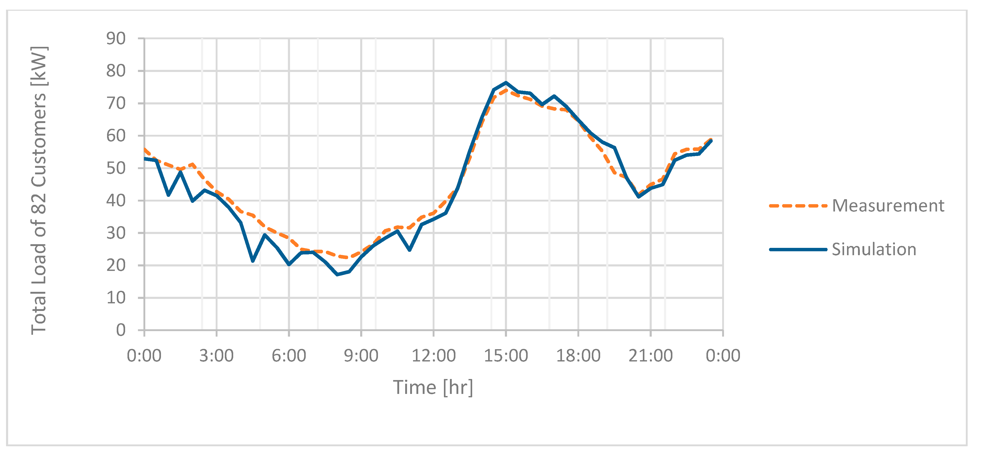
Figure 9 illustrates the comparison between simulation results and measurement results in the sample grid with the specifications given in Table 1 to validate the model. Measurement results belong to the mean days of 16 July to 10 August 2019 [53]. Due to the different behavior of subscribers on holidays and semi-holidays, weekends are omitted on average load behavior calculations. Simulation results are obtained with one-minute accuracy, but they need to be calculated in the form of 30 min sets, since the measurements were made in 30 min intervals.
To calculate the amount of error between the simulation results and the measurement results, the values of normalized root mean square error (), normalized mean absolute error () and relative mean error () are calculated as follows [54]:
where and are the values obtained from the simulation and the measured values respectively. Also represents the number of values to be compared.
The calculated values of , , and are 8.89%, 6.19% and 7.42%, respectively. The average magnitude of the absolute values of simulation errors is 4.69%. The average daily energy consumption measured is 13.51 kWh per customer compared to 13.03 kWh as the average daily energy consumption per customer obtained from the simulation, which shows a difference of approximately 3.5%.
5.3. Simulation of the Effect of Grid-Connected Photovoltaic Resources
It is assumed that 10% of subscribers will use grid-connected photovoltaic panels to supply their required energy and sell their surplus energy to the global grid. Considering the average floor area of homes of the studied town and the on-grid inverter panels and inverters available in the market, the rated power of 1, 1.5 and 2 kW grid PV systems is considered. The characteristics of the simulated modules in this study are described in Table 3. The specifications given in Table 3 are specific to standard temperature conditions (25 °C) and the increase in temperature reduces the efficiency of the photovoltaic module [55,56]. The effect of temperature on the output power of the PV module is modeled by coefficients µIsc and µVoc. The performance factor (PR) depends on a number of factors, including inverter losses, AC and DC cable losses, shadow or cloud output power loss, and reduced efficiency caused by dust and snow on the modules.
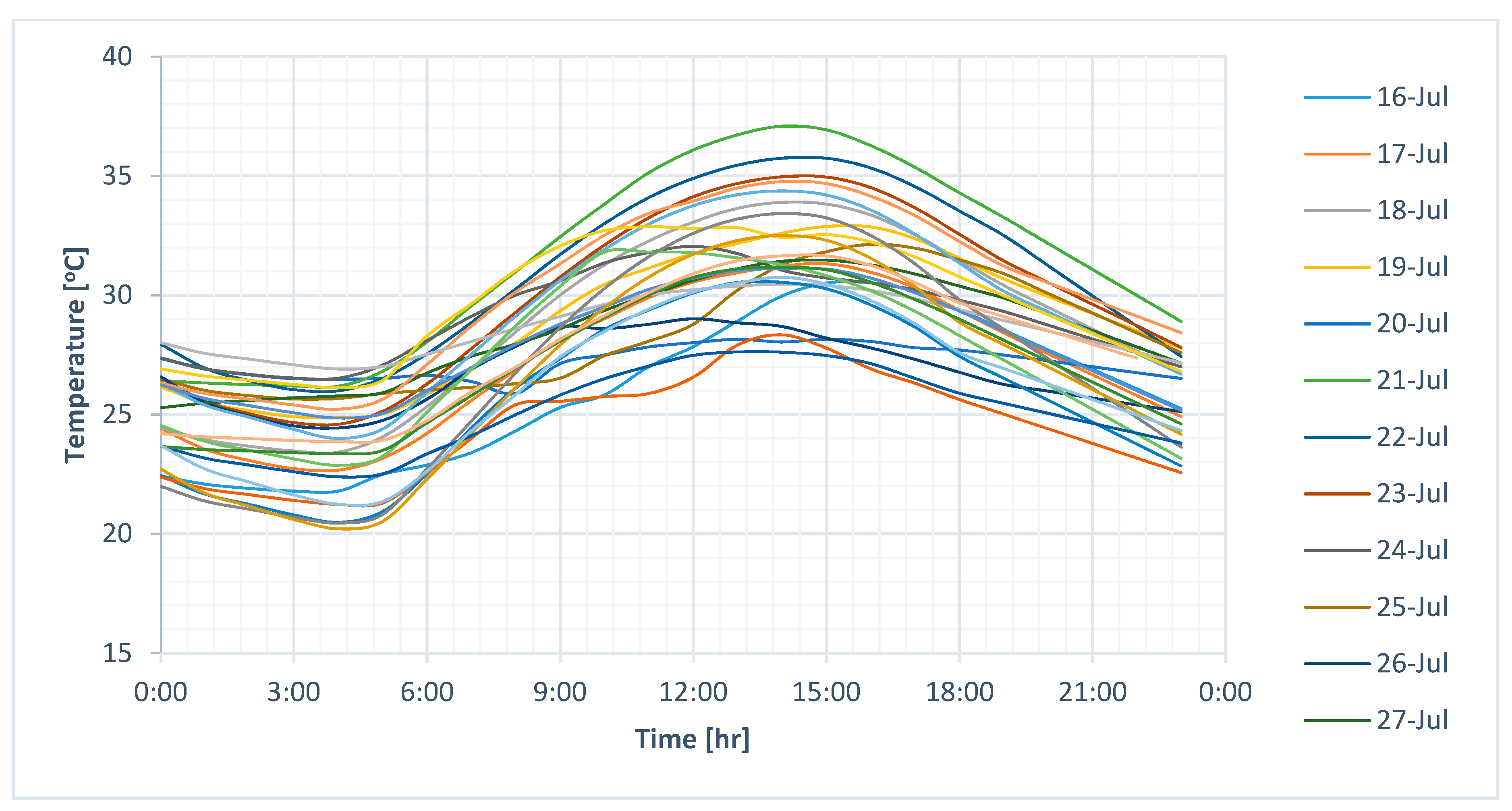
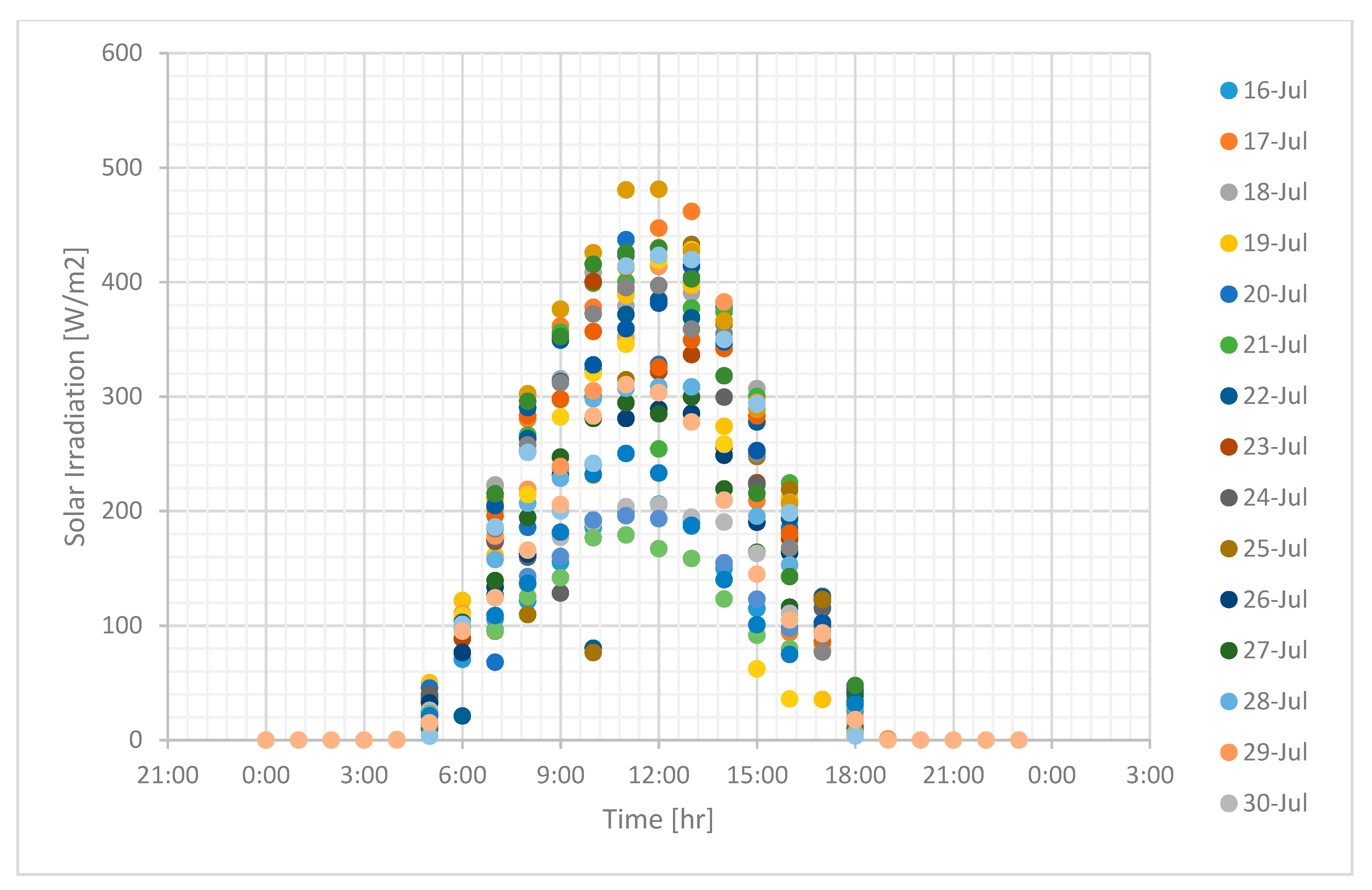
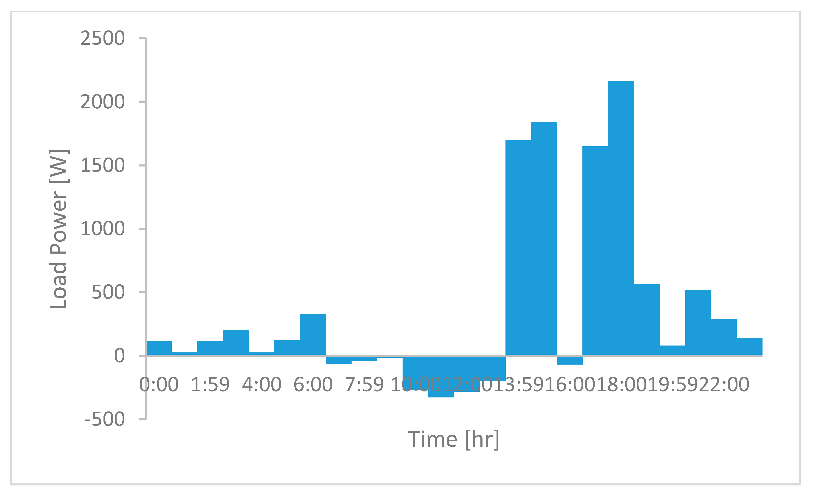
The temperature profile and the amount of solar radiation power are other required data. These data are available with a maximum resolution of 1 h (Figure 10 and Figure 11). As shown in Figure 10, the solar radiation power in the study period is very diffuse and variable. The reason for this is the proximity of the city under study to the Caspian Sea and, as a result, high cloud changes. The effect of these drastic changes is modeled with the help of the performance factor (PR). In this study, the PR value is assumed to follow a normal probability distribution in the range of the numbers given in Table 3. The load profile of a sample customer with a PV module is shown in Figure 12. The photovoltaic panel connected to this particular customer is intended as 1 kW. At certain times, the customer load profile goes negative. This is due to the times when the amount of power generated by the PV exceeds the load consumed and the customer delivers surplus power to the grid.
Customers equipped with a grid-connected PV are connected to the grid in two ways; one is a customer whose photovoltaic panels are connected directly to the grid via the inverter and then the energy meter. All the solar energy generated by these customers is sold to the grid in the retail market. These customers purchase all their needed electricity from the global network. This type of connection is used in cases where the energy generated by the customer is purchased from the customer at a price higher than the energy sales tariffs, in order to encourage the development of renewable energy production. Obviously, these customers fall into the category of subscribers without PV in terms of load behavior analysis. The second category is customers who self-supply by PV power and deliver surplus electricity to the grid. In the analysis performed in this study, these customers, which are connected to the global network by means of bi-directional meters, fall into the clusters of PV-equipped subscribers. In fact, the load profile of these subscribers is the result of subtracting the consumption and the production power.
Iran’s National Smart Metering Program, known as FAMAM, collects the metering data every 15 min. Although simulation results are available with a resolution of one minute, the simulations of the load behavior are appropriately adapted for 15 min intervals.
5.4. Mass Data Generation
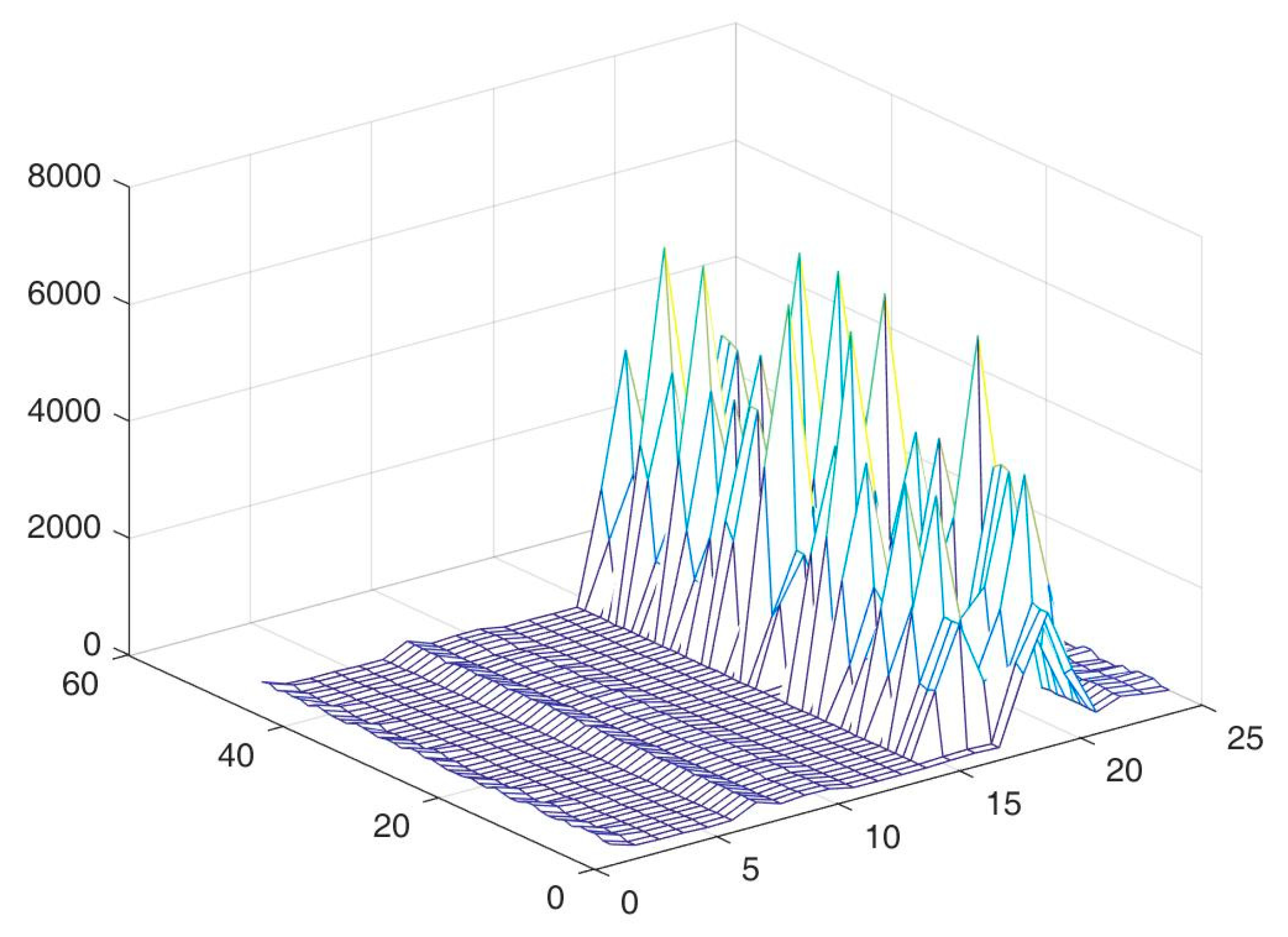
In order to better train the neural network used in the analysis, 5000 load profiles were generated using the proposed models and simulation. Ten percent of these subscribers receive part of their energy from rooftop photovoltaic panels and sell surplus generation power to the grid through the retail market. Using the initial mass data generated from simulation to train the SOM neural network does not lead to an analyzable result. One of the reasons is the high number of elements of the input matrix. Clustering of 15 min load curves has little convergence in addition to the high computational cost. On the other hand, since the curves of the solar radiation are available on an hourly average, virtually a 15 min load curve analysis will not have a significant effect on the accuracy of the simulation. By clustering the mass-produced curves, the load behavior curves of non-PV customers fall into 22 clusters and the PV-connected load profiles fall into 26 clusters with different characteristics as shown in Figure 13.
5.5. Fraud Detection
The anomalies of power distribution networks fall into five categories:
- Malfunctioning meters.
- Customers who bypass the meter at certain hours.
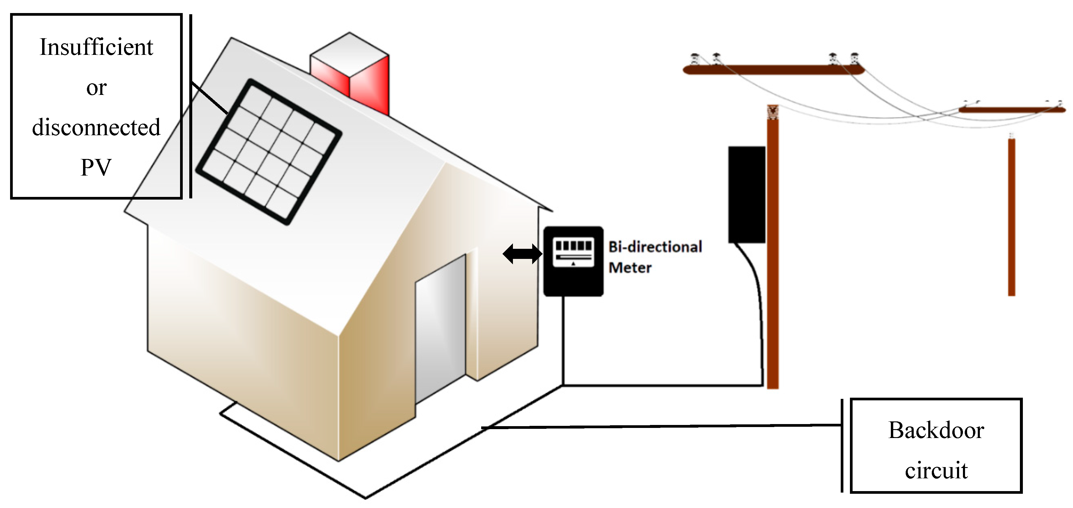
- Customers who consume part of their loads through an unmetered circuit at certain hours of the day (Figure 14).
- Subscribers who disable the meter on some days in each reading period (specific for old electromagnetic meters).
- Customers who receive electricity from the grid across a circuit other than the meter and deliver it to the grid as photovoltaic energy. (This happens in cases where incentives are being made to buy renewable energy at a price higher than the cost of selling electricity to customers) (Figure 15).
Each of these types of anomaly leads to different behavior in the load profile curve and the amount of customers’ energy consumption. For example, the consumption curve of customers who have defective meters, while maintaining approximately the behavioral pattern of normal customers, is higher or lower; or, in the case of customers who use conventional meters that cannot be read online, manipulating the meter on a number of days per meter reading period will reduce the total energy measured.
5.5.1. Early Detection of Abnormalities/Fraud
For customers who use conventional electromagnetic meters, instantaneous data is not available and the only accessible data is the energy consumption for a given period. Ancillary data such as period of consumption, number of days of consumption, and postal area (representing welfare level) are valuable data in this regard. In the city of Galougah’s network, in particular, the customers carefully monitored in these studies use either electromagnetic meters or digital meters not connected to the national smart metering system (FAHAM). The energy consumption data of these customers is available in different periods and years along with the test results of the meters. This information is valuable for evaluating the effectiveness of the present studies.
To analyze anomalies/fraud in this subset of customers, mass energy consumption data is generated at different times with the time tag and used to train the SOM neural network. Then, real network data is used as test data. It is interesting to compare the results of the proposed method with the results of the meter inspection. Of the 82 customers evaluated, 14 were recognized as suspected of malformations. Table 4 shows the comparison of the simulation result and the inspection result for the meters. The algorithm was not successful at detecting 2 of the actual frauds among target customers. This occurred due to similarity of the two customers to less energy-consuming customers. This error may be extinguished by adding some extra labels such welfare level to the ANN-network input data. There is also a mis-detection where a customer with no fraud was detected as suspected. This normally happens for customers with fully different consumption behavior of which load behavior cannot be assigned to any load clusters.
5.5.2. Detection of Fraud in Customers Connected to AMI (Automatic Meter Reading) System
No test data is available for this group of subscribers. Therefore, a deliberate anomaly is imposed on the consumption curve of these customers, to test the performance of the proposed method. Table 5 describes the process and volume of deliberate anomalies created in the consumption data. The results of the fraud detection analysis for smartly metered customers are presented in Table 6.
6. Conclusions
The purpose of this study is to present a method for detecting fraud as the most important non-technical factor in distribution network losses. Distribution networks with high penetration of grid-connected photovoltaic sources have been specifically investigated in this study. Using a bottom-up model, the normal load behavior of customers is generated. Simulation is used to determine the effect of widespread use of grid-connected photovoltaic sources on the load profile of domestic customers.
Load profile curves in the presence of grid-connected photovoltaic units are generated using simulation. Clustering of these curves using a self-organized neural network (SOM) determines normal load behavior patterns. Based on the fuzzy logic model, the Euclidean distance of any load profile to the center of the nearest normal cluster is calculated as the index of anomaly of the corresponding customer. The mechanism for detecting where the non-technical losses occur is different in networks with conventional electromagnetic meters to those in smart grids. A survey conducted to identify customers suspected of energy theft had successful results in both groups. The proposed algorithm has also shown great performance in detecting types of fraud in smart electrical networks, including: bypassing meters at specific hours, supplying part of the energy through an unmetered circuit, and selling non-photovoltaic energy as photovoltaic to the grid.
Author Contributions
Conceptualization, A.K. and A.V.; methodology, A.K. and H.M.; software, A.V.; validation, A.K.; formal analysis, A.K. and A.V.; investigation, A.V.; resources, A.A.; data curation, A.V.; writing—original draft preparation, A.V.; writing—review and editing, A.V., A.K..; visualization, A.V.; supervision, A.K., H.M., and A.A.; project administration, A.K.; All authors have worked on this manuscript together and all authors have read and approved the final manuscript.
Funding
This research received no external funding.
Conflicts of Interest
The authors declare no conflict of interest.
Nomenclatures
| Probability of the appliance turning on at each time step | |
| Indicator of home appliance | |
| Calculation time step | |
| Time in hours | |
| Frequency of appliance turning on in terms of number of times | |
| Scaling factor that scales probabilities on the basis of | |
| PV module output current | |
| Number of cells in parallel | |
| Generated current by solar radiation | |
| Reverse saturation current | |
| Charge of an electron | |
| PV module output voltage | |
| Diode ideality factor | |
| The Boltzmann’s constant | |
| Temperature of the PV module in K | |
| Current due to intrinsic shunt resistance of the PV module | |
| Reference temperature | |
| Saturation current at reference temperature () | |
| The band-gap energy | |
| It | Short-circuit current temperature coefficient |
| Short-circuit current of PV module | |
| Number of cells in series | |
| Internal shunt resistance of the PV module | |
| The ith input vector of neural network | |
| The weight vector which connects the ith input to the jth output | |
| A map unit | |
| The solar insolation | |
| Previous weight vector between input vector and weight vector to output neuron j | |
| Updated weight vector between input cell i and output cell j | |
| Neighboring function | |
| The distance of the ith load curve from the center of the jth cluster | |
| t | Time of the day |
| The load of the ith customer at time t | |
| The load of the center of the jth cluster at time t | |
| The number of clusters | |
| The membership of any customers to normal behavior | |
| Nominal power of each appliance [W] | |
| Standby power of each appliance [W] | |
| Number of appliances in each home | |
| The average time period that each appliance keeps on | |
| Normalized root mean square error | |
| Normalized mean absolute error | |
| Relative mean error | |
| Values obtained from simulation | |
| Values obtained from measurement | |
| Number of values |
References
- TAVANIR. Detailed Statistics on Iran’s Power Distribution Networks in 1396; TAVANIR: Tehran, Iran, 2018; Volume 1. [Google Scholar]
- Cabral, J.; Gontijo, E.M. Fraud detection in electrical energy consumers using rough sets. In Proceedings of the 2004 IEEE International Conference on Systems, Man and Cybernetics, Hague, The Netherlands, 10–13 October 2004; pp. 3625–3629. [Google Scholar]
- Cabral, J.E.; Pinto, J.O.; Pinto, A.M. Fraud detection system for high and low voltage electricity consumers based on data mining. In Proceedings of the 2009 IEEE Power & Energy Society General Meeting, Calgary, AB, Canada, 26–30 July 2009; pp. 1–5. [Google Scholar]
- Monedero, I.; Biscarri, F.; Leon, C.; Biscarri, J.; Millan, R. MIDAS: Detection of Non-Technical Losses in Electrical Consumption Using Neural Networks and Statistical Techniques. Comput. Vis. 2006, 3984, 725–734. [Google Scholar]
- Viegas, J.; Esteves, P.R.; Melicio, R.; Mendes, V.; Vieira, S.M. Solutions for detection of non-technical losses in the electricity grid: A review. Renew. Sustain. Energy Rev. 2017, 80, 1256–1268. [Google Scholar] [CrossRef] [Green Version]
- Han, W.; Xiao, Y. NFD: Non-technical loss fraud detection in smart grid. Comput. Secur. 2017, 65, 187–201. [Google Scholar] [CrossRef] [Green Version]
- Abaide, A.; Canha, L.; Barin, A.; Cassel, G. Assessment of the smart grids applied in reducing the cost of distribution system losses. In Proceedings of the 2010 7th International Conference on the European Energy Market, Madrid, Spain, 23–25 June 2010; Institute of Electrical and Electronics Engineers (IEEE): Piscataway, NJ, USA; pp. 1–6. [Google Scholar]
- Jiang, R.; Lu, R.; Wang, Y.; Luo, J.; Shen, C.; Shen, X. Energy-theft detection issues for advanced metering infrastructure in smart grid. Tsinghua Sci. Technol. 2014, 19, 105–120. [Google Scholar] [CrossRef]
- Mashima, D.; Cárdenas, A.A. Evaluating Electricity Theft Detectors in Smart Grid Networks. In International Workshop on Recent Advances in Intrusion Detection; Springer: Berlin/Heidelberg, Germany, 2012; Volume 7462, pp. 210–229. [Google Scholar]
- Dickert, J.; Schegner, P. Residential load models for network planning purposes. In Proceedings of the 2010 Modern Electric Power Systems, Wroclaw, Poland, 20–22 September 2010; pp. 1–6. [Google Scholar]
- Nickel, D.; Braunstein, H. Distribution transformer loss evaluation: II-load characteristics and system cost parameters. IEEE Trans. Power Appar. Syst. 1981, 2, 798–811. [Google Scholar] [CrossRef]
- Capasso, A.; Grattieri, W.; LaMedica, R.; Prudenzi, A. A bottom-up approach to residential load modeling. IEEE Trans. Power Syst. 1994, 9, 957–964. [Google Scholar] [CrossRef]
- Chuan, L.; Ukil, A. Modeling and validation of electrical load profiling in residential buildings in Singapore. IEEE Trans. Power Syst. 2014, 30, 2800–2809. [Google Scholar] [CrossRef] [Green Version]
- Gao, B.; Liu, X.; Zhu, Z. A bottom-up model for household load profile based on the consumption behavior of residents. Energies 2018, 11, 2112. [Google Scholar] [CrossRef] [Green Version]
- Gruber, J.; Jahromizadeh, S.; Prodanovic, M.; Rakočević, V. Application-oriented modelling of domestic energy demand. Int. J. Electr. Power Energy Syst. 2014, 61, 656–664. [Google Scholar] [CrossRef] [Green Version]
- Gils, H.C. Assessment of the theoretical demand response potential in Europe. Energy 2014, 67, 1–18. [Google Scholar] [CrossRef]
- Munkhammar, J.; Rydén, J.; Widén, J. Characterizing probability density distributions for household electricity load profiles from high-resolution electricity use data. Appl. Energy 2014, 135, 382–390. [Google Scholar] [CrossRef]
- Swan, L.G.; Ugursal, V.I. Modeling of end-use energy consumption in the residential sector: A review of modeling techniques. Renew. Sustain. Energy Rev. 2009, 13, 1819–1835. [Google Scholar] [CrossRef]
- Paatero, J.; Lund, P. A model for generating household electricity load profiles. Int. J. Energy Res. 2006, 30, 273–290. [Google Scholar] [CrossRef] [Green Version]
- Widén, J.; Lundh, M.; Vassileva, I.; Dahlquist, E.; Ellegård, K.; Wäckelgård, E. Constructing load profiles for household electricity and hot water from time-use data—Modelling approach and validation. Energy Build. 2009, 41, 753–768. [Google Scholar] [CrossRef]
- Widén, J.; Munkhammar, J. Evaluating the benefits of a solar home energy management system: Impacts on photovoltaic power production value and grid interaction. In Proceedings of the ECEEE 2013 Summer Study, Presqu’île de Giens, France, 3–8 June 2013. [Google Scholar]
- Widén, J.; Molin, A.; Ellegård, K. Models of domestic occupancy, activities and energy use based on time-use data: Deterministic and stochastic approaches with application to various building-related simulations. J. Build. Perform. Simul. 2012, 5, 27–44. [Google Scholar] [CrossRef]
- Richardson, I.; Thomson, M.; Infield, D. A high-resolution domestic building occupancy model for energy demand simulations. Energy Build. 2008, 40, 1560–1566. [Google Scholar] [CrossRef] [Green Version]
- Richardson, I.; Thomson, M.; Infield, D.; Delahunty, A. Domestic lighting: A high-resolution energy demand model. Energy Build. 2009, 41, 781–789. [Google Scholar] [CrossRef] [Green Version]
- Widén, J.; Nilsson, A.M.; Wäckelgård, E. A combined Markov-chain and bottom-up approach to modelling of domestic lighting demand. Energy Build. 2009, 41, 1001–1012. [Google Scholar] [CrossRef]
- Widén, J.; Wäckelgård, E. A high-resolution stochastic model of domestic activity patterns and electricity demand. Appl. Energy 2010, 87, 1880–1892. [Google Scholar] [CrossRef]
- Richardson, I.; Thomson, M.; Infield, D.; Clifford, C. Domestic electricity use: A high-resolution energy demand model. Energy Build. 2010, 42, 1878–1887. [Google Scholar] [CrossRef] [Green Version]
- Kavgic, M.; Mavrogianni, A.; Mumovic, D.; Summerfield, A.; Stevanovic, Z.; Djurovic-Petrovic, M. A review of bottom-up building stock models for energy consumption in the residential sector. Build. Environ. 2010, 45, 1683–1697. [Google Scholar] [CrossRef]
- Omran, W.A.; Kazerani, M.; Salama, M.M.A. Investigation of methods for reduction of power fluctuations generated from large grid-connected photovoltaic systems. IEEE Trans. Energy Convers. 2010, 26, 318–327. [Google Scholar] [CrossRef]
- Datta, M.; Senjyu, T.; Yona, A.; Funabashi, T.; Kim, C.-H. A frequency-control approach by photovoltaic generator in a PV–diesel hybrid power system. IEEE Trans. Energy Convers. 2010, 26, 559–571. [Google Scholar] [CrossRef]
- Abdolzadeh, M.; Zarei, T. Optical and thermal modeling of a photovoltaic module and experimental evaluation of the modeling performance. Environ. Prog. Sustain. Energy 2016, 36, 277–293. [Google Scholar] [CrossRef]
- Houari, Z.M.; Zohra, Z.F.; Mansour, Z.; Amar, T. Photovoltaic solar array: Modeling and output power optimization. Environ. Prog. Sustain. Energy 2016, 35, 1529–1536. [Google Scholar] [CrossRef]
- Lokesh, T.; Srinivasa, D.; Srinath, M.S. Review on MPPT techniques for solar PV array system. Our Herit. 2020, 68, 7887–7894. [Google Scholar]
- Singh, B.P.; Goyal, S.K.; Siddiqui, S.A. Analysis and Classification of Maximum Power Point Tracking (MPPT) Techniques: A Review. In Lecture Notes in Electrical Engineering; Springer: Berlin/Heidelberg, Germany, 2019; pp. 999–1008. [Google Scholar]
- Mahdi, A.S.; Mahamad, A.K.; Saon, S.; Tuwoso, T.; Elmunsyah, H.; Mudjanarko, S.W. Maximum power point tracking using perturb and observe, fuzzy logic and ANFIS. SN Appl. Sci. 2019, 2, 89. [Google Scholar] [CrossRef] [Green Version]
- Ahmed, J.; Chin, V.J. An improved perturb and observe (P&O) maximum power point tracking (MPPT) algorithm for higher efficiency. Appl. Energy 2015, 150, 97–108. [Google Scholar]
- Sera, D.; Mathe, L.; Kerekes, T.; Spataru, S.; Teodorescu, R. On the Perturb-and-Observe and Incremental Conductance MPPT Methods for PV Systems. IEEE J. Photovolt. 2013, 3, 1070–1078. [Google Scholar] [CrossRef]
- De Brito, M.A.; Sampaio, L.P.; Luigi, G.; Melo, G.A.; Canesin, C.A. Comparative analysis of MPPT techniques for PV applications. In Proceedings of the 2011 International Conference on Clean Electrical Power (ICCEP), Ischia, Italy, 14–16 June 2011; pp. 99–104. [Google Scholar]
- Pourgharibshahi, H.; Abdolzadeh, M.; Fadaeinedjad, R. Verification of computational optimum tilt angles of a photovoltaic module using an experimental photovoltaic system. Environ. Prog. Sustain. Energy 2014, 34, 1156–1165. [Google Scholar] [CrossRef]
- Raj, M.P.; Joshua, A.M. Design, implementation and performance analysis of a LabVIEW based fuzzy logic MPPT controller for stand-alone PV systems. In Proceedings of the 2017 IEEE International Conference on Power, Control, Signals and Instrumentation Engineering (ICPCSI), Chennai, India, 21–22 September 2017; pp. 1012–1017. [Google Scholar]
- Boumaaraf, H.; Talha, A.; Bouhali, O. A three-phase NPC grid-connected inverter for photovoltaic applications using neural network MPPT. Renew. Sustain. Energy Rev. 2015, 49, 1171–1179. [Google Scholar] [CrossRef]
- Ramaprabha, R.; Mathur, B. Genetic algorithm based maximum power point tracking for partially shaded solar photovoltaic array. Int. J. Res. Rev. Inf. Sci. 2012, 2, 161–163. [Google Scholar]
- Ishaque, K.; Chin, V.J.; Amjad, M.; Mekhilef, S. An Improved Particle Swarm Optimization (PSO)–Based MPPT for PV with Reduced Steady-State Oscillation. IEEE Trans. Power Electron. 2012, 27, 3627–3638. [Google Scholar] [CrossRef]
- Atiq, J.; Soori, P.K. Modelling of a grid connected solar PV system using MATLAB/Simulink. Int. J. Simul. Syst. Sci. Technol. 2017, 17, 451–457. [Google Scholar]
- Fayyad, U.; Piatetsky-Shapiro, G.; Smyth, P. From data mining to knowledge discovery in databases. Al Mag. 1996, 17, 37. [Google Scholar]
- Piatetsky-Shapiro, G. Knowledge discovery in real databases: A report on the IJCAI-89 Workshop. Al Mag. 1990, 11, 68. [Google Scholar]
- Cabral, J.E.; Pinto, J.O.P.; Martins, E.M.; Pinto, A.M.A.C. Fraud detection in high voltage electricity consumers using data mining. In Proceedings of the 2008 IEEE/PES Transmission and Distribution Conference and Exposition, Chicago, IL, USA, 21–24 April 2008; Institute of Electrical and Electronics Engineers (IEEE): Piscataway, NJ, USA; pp. 1–5. [Google Scholar]
- Alvarez-Guerra, E.; Molina, A.; Viguri, J.; Alvarez-Guerra, M. A SOM-based methodology for classifying air quality monitoring stations. Environ. Prog. Sustain. Energy 2010, 30, 424–438. [Google Scholar] [CrossRef]
- Orsi Noor Consultant Engineers, O.N.C. Mazandaran Galougah Power Distribution Network Master Planning-Load Modelling. In Engineering; Mazandaran Power Distribution Co.: Amir Mazandarani, Iran, 2017; Volume 01. [Google Scholar]
- Orsi Noor Consultant Engineers, O.N.C. Mazandaran Galougah Power Distribution Network Master Planning-Load Forecasting. In Engineering; Mazandaran Power Distribution Co.: Amir Mazandarani, Iran, 2017; Volume 01. [Google Scholar]
- SATBA. Share of Household Energy Consumption; Eurostat: Brussels, Belgium, 2013. [Google Scholar]
- Laicane, I.; Blumberga, D.; Blumberga, A.; Rosa, M. Evaluation of Household Electricity Savings. Analysis of Household Electricity Demand Profile and User Activities. Energy Procedia 2015, 72, 285–292. [Google Scholar] [CrossRef] [Green Version]
- Engineers, O.N.C. Modern Engineering and Technology Development Studies: Engineering Studies on Development, Modification and Optimization of Mazandaran Power Distribution Networks. In Engineering; Mazandaran Power Distribution Co.: Amir Mazandarani, Iran, 2019; Volume 01. [Google Scholar]
- Kasaeian, A.; Barghamadi, H.; Pourfayaz, F. Performance comparison between the geometry models of multi-channel absorbers in solar volumetric receivers. Renew. Energy 2017, 105, 1–12. [Google Scholar] [CrossRef]
- Poulek, V.; Matuska, T.; Libra, M.; Kachalouski, E.; Sedláček, J. Influence of increased temperature on energy production of roof integrated PV panels. Energy Build. 2018, 166, 418–425. [Google Scholar] [CrossRef]
- Libra, M.; Beránek, V.; Sedláček, J.; Poulek, V.; Tyukhov, I. Roof photovoltaic power plant operation during the solar eclipse. Sol. Energy 2016, 140, 109–112. [Google Scholar] [CrossRef]
Figure 1.
The bottom-up load modeling diagram.

Figure 2.
The equivalent circuit of a photovoltaic (PV) module [30].
Figure 2.
The equivalent circuit of a photovoltaic (PV) module [30].

Figure 3.
Block diagram of maximum power point tracking (MPPT) model.

Figure 4.
The structure of self-organized neural network (SOM) network.

Figure 5.
Flowchart of proposed method for fraud detection in power distribution networks.

Figure 6.
Domestic load density of Galougah [50].
Figure 6.
Domestic load density of Galougah [50].

Figure 7.
The start-on probability distribution of home appliances. (a) Microwave Oven; (b) Refrigerator; (c) Coffee Maker; (d) Clothes Washing Machine; (e) Regular Kitchen Appliances; (f) TV; (g) Laptops and PCs; (h) Gaming Tools; (i) Cooling; (j) Hair Drying; (k) Lighting; (l) Electric Kettle; (m) Dish Washer; (n) Clothes Ironing; (o) Cooling and Ventilation fans; (p) Battery Chargers and Voltage Adaptors.


Figure 8.
(a)–(d) Simulation result: load profiles of four common samples with four different load profile types.
Figure 8.
(a)–(d) Simulation result: load profiles of four common samples with four different load profile types.

Figure 9.
Comparison of load profile measurement results and simulation results.

Figure 10.
Temperature profiles for the study days.

Figure 11.
The amount of sunlight radiation during the days under study.

Figure 12.
Load profile of a sample customer with grid-connected PV.

Figure 13.
All cluster centers of mass data.

Figure 14.
Illustration of energy theft through unmetered circuits.

Figure 15.
Illustration of energy fraud through energy selling.


Table 1.
Specifications of the data logger installation point.
| Substation Name | Transformer Nominal Capacity (kVA) | Customer Classes | |||
|---|---|---|---|---|---|
| Domestic | Public | Industrial | Commercial and Other | ||
| Zeytoon Complex | 160 | 76 | 2 | - | 4 |
Table 2.
Power consumption characteristics of household electrical appliances.
| Appliance | Appliance Saturation | Nominal Wattage [W] | Standby [W] | Mean Daily Starting Frequency [f] | Time Per Cycle [min] |
|---|---|---|---|---|---|
| Microwave Oven | 0.2 | 1500 | - | 5 | 2 |
| Refrigerator | 1 | 180 | 10 | 44.5 | 15 |
| Coffee Maker | 0.1 | 1200 | - | 0.76 | 6 |
| Clothes Washer | 0.75 | 2000 | - | 0.22 | 65 |
| Other Kitchen Appliance | 0.2 | 300 | - | 0.1 | 10 |
| TV | 1 | 180 | 10 | 2 | 120 |
| PC and Laptop | 0.92 | 110 | 3 | 2.5 | 70 |
| Gaming Tools | 0.22 | 100 | 2 | 1 | 120 |
| Air Conditioner | 0.9 | 2100 | - | 2 | 120 |
| Hair Dryer | 1 | 1200 | - | 0.2 | 7 |
| Lighting | 1 | 160 | - | 10 | 30 |
| Electric Kettle | 0.4 | 480 | - | 2 | 6 |
| Dish Washer | 0.15 | 2000 | - | 0.14 | 190 |
| Iron | 1 | 1700 | - | 0.3 | 7 |
| Cooling and Ventilation fans | 0.91 | 80 | - | 1 | 120 |
| Battery Chargers and Voltage Adaptors | 1 | 5 | - | 3 | 60 |
| Electric Water Heating | 0 | 2000 | - | - | - |
Table 3.
Specifications of the simulated PV module.
| Nominal Power [W] | Technology | Maximum Power | Temperature Coefficient | Size [mm × mm] | Efficiency [%] | Performance Ratio [PR] | ||
|---|---|---|---|---|---|---|---|---|
| Impp [A] | Vmpp [V] | µIsc [mA/°C] | µVoc [mV/°C] | |||||
| 250 | Si-poly | 8.330 | 30.0 | 4.3 | −137 | 1640 × 992 | 15.3 | 0.5−0.9 |
Table 4.
Comparison of simulation results and test results for meters of study area.
| Meter Code | Measurement Error (Inspection Result) [%] | The Calculated Value of the Degree of Anomaly [1,2,3,4,5,6,7,8,9] | Validation Result |
|---|---|---|---|
| 23***26 | 22% | 4 | Detected |
| 23***39 | 8% | 2 | Detected |
| 23***56 | 25% | 4 | Detected |
| 23***94 | 9% | 0 | Not detected |
| 23***22 | 27% | 4 | Detected |
| 23***05 | 10% | 3 | Detected |
| 23***27 | 16% | 3 | Detected |
| 23***02 | 22% | 0 | Not detected |
| 23***63 | 17% | 3 | Detected |
| 23***16 | 81% | 9 | Detected |
| 23***94 | 3% | 3 | Mis-detected |
| 23***32 | 29% | 6 | Detected |
| 24***80 | 25% | 5 | Detected |
| 23***18 | 66% | 7 | Detected |
Table 5.
Modeling anomaly of customers connected to smart meters.
| Type of Fraud | Modeling Method | Class of Anomaly | Number of Frauding Customers |
|---|---|---|---|
| The customer bypasses the meter at specified hours | The customer’s load becomes zero at random periods | A | 1% of PV and 1% of non-PV customers |
| The customer consumes part of his loads through an unmetered circuit at certain hours | The customer’s load reaches 70% of normal load at random periods | B | 1% of PV and 1% of non-PV customers |
| The customer sells the grid energy as PV energy | A power supply with controllable power is considered on the load side | C | 1% of PV customers |
Table 6.
Result of fraud detection analysis in customers with smart meters.
| Class of Anomaly | Percent of Detected Frauds | Percent of Mistakenly Detected Frauds | Average Degree of Anomaly in Reference Data | Average Detected Degree of Anomaly in Records |
|---|---|---|---|---|
| A | 64 | 2.23 | 6 | 7 |
| B | 49 | 2.61 | 4 | 3 |
| C | 91 | 1.04 | 4 | 5 |
© 2020 by the authors. Licensee MDPI, Basel, Switzerland. This article is an open access article distributed under the terms and conditions of the Creative Commons Attribution (CC BY) license (http://creativecommons.org/licenses/by/4.0/).
Share and Cite
MDPI and ACS Style
Vahabzadeh, A.; Kasaeian, A.; Monsef, H.; Aslani, A. A Fuzzy-SOM Method for Fraud Detection in Power Distribution Networks with High Penetration of Roof-Top Grid-Connected PV. Energies 2020, 13, 1287. https://doi.org/10.3390/en13051287
AMA Style
Vahabzadeh A, Kasaeian A, Monsef H, Aslani A. A Fuzzy-SOM Method for Fraud Detection in Power Distribution Networks with High Penetration of Roof-Top Grid-Connected PV. Energies. 2020; 13(5):1287. https://doi.org/10.3390/en13051287
Chicago/Turabian StyleVahabzadeh, Alireza, Alibakhsh Kasaeian, Hasan Monsef, and Alireza Aslani. 2020. "A Fuzzy-SOM Method for Fraud Detection in Power Distribution Networks with High Penetration of Roof-Top Grid-Connected PV" Energies 13, no. 5: 1287. https://doi.org/10.3390/en13051287
Note that from the first issue of 2016, this journal uses article numbers instead of page numbers. See further details here.