An Ensemble Forecasting Model of Wind Power Outputs Based on Improved Statistical Approaches


Department of Energy Grid, Sangmyung University, Seoul 03016, Korea
*
Author to whom correspondence should be addressed.
Energies 2020, 13(5), 1071; https://doi.org/10.3390/en13051071
Submission received: 28 January 2020
/
Revised: 24 February 2020
/
Accepted: 25 February 2020
/
Published: 1 March 2020
(This article belongs to the Special Issue Enhanced Variable Renewable Energies Forecasts for Optimal Grid Operations)
Abstract
:The number of wind-generating resources has increased considerably, owing to concerns over the environmental impact of fossil-fuel combustion. Therefore, wind power forecasting is becoming an important issue for large-scale wind power grid integration. Ensemble forecasting, which combines several forecasting techniques, is considered a viable alternative to conventional single-model-based forecasting for improving the forecasting accuracy. In this work, we propose the day-ahead ensemble forecasting of wind power using statistical methods. The ensemble forecasting model consists of three single forecasting approaches: autoregressive integrated moving average with exogenous variable (ARIMAX), support vector regression (SVR), and the Monte Carlo simulation-based power curve model. To apply the methodology, we conducted forecasting using the historical data of wind farms located on Jeju Island, Korea. The results were compared between a single model and an ensemble model to demonstrate the validity of the proposed method.
1. Introduction
With limits to fossil fuel reserves and the emerging importance of environmental protection around the world, renewable energy sources have received considerable attention. Among them, wind power is considered a front-runner for increasing the global installed capacity of renewable power facilities. In 2018, global renewable energy capacity grew to ~2378 GW; wind power accounts for 28% of the additional renewable capacity [1]. Global installed wind power capacity reached 579 GW, and, according to estimates, wind power will supply over 20% of total global power by 2030 [2]. As wind power generation increases within power systems, the penetration of wind power presents many challenges to system operators. The high penetration of wind power affects real-time system operations, the quality of power, and the reliability of power systems [3,4]. As wind power generation output is variable and intermittent, depending on weather conditions, supplying wind power continuously and reliably by using wind power forecasting is essential. Accurate wind power forecasting improves energy conversion efficiency and reduces the risk of overload, thereby enabling reliable system operation [5].
In various studies, a number of methods have been successfully applied to forecast wind power. Wind power forecasting models are divided into three main categories: physical models, statistical models, and combinations of both [6,7]. The physical model uses physical considerations based on the lower atmosphere or numerical weather prediction (NWP), using weather forecast information such as temperature, pressure, and obstacles [8]. Generally, when using wind speed obtained from a local weather service, the speed is adjusted to the onsite conditions at the wind farm and then converted to power output through the power curve [9]. Shokrzadeh et al. propose the wind turbine power curve estimation through polynomial regression—a statistical technique [10]. Statistical models basically use the relationships of historical data to perform short-term forecasts. Compared to other models, these models are easier and cheaper to develop, but the forecast error increases proportionally with the forecast time. Typical statistical models include the autoregressive (AR), autoregressive moving average (ARMA), and autoregressive integrated moving average (ARIMA) and are used for small forecast horizons [11]. Wang et al. propose a Bayesian-based adaptive multi-kernel regression model [12]. Shi et al. compare ARIMA, an artificial neural network (ANN) and a support vector machine (SVM) [13]. Time-series forecasting models including the ARIMA model explicitly represent the relationship between inputs and outputs but are limited in linear components. Artificial intelligence (AI) and machine learning (ML) approaches are suitable for modeling nonlinear components but are computationally intensive, and outputs are difficult to understand. Statistical models can be used in combination with NWP models. Statistical models may have significant accuracy in very-short-term forecasting (3–4 h). However, owing to the increased errors produced over time, statistical models are used in combination with physical models as a practical alternative for improving forecast accuracy [14]. These forecasting methods are summarized in Table 1 [3].
Wind power forecasting is classified into very-short-term, short-term, medium-term and longer-term according to the timescale [15,16]. Table 2 shows the time horizons and the scope of application for each of the four categories. This work proposes short-term wind power forecasting through a combination of several statistical techniques. The models proposed here include autoregressive integrated moving average with exogenous variables (ARIMAX), support vector regression (SVR), and the Monte-Carlo simulation (MCS) power curve models. The forecasting uses wind power output data and wind-speed data. Through spatial modeling, wind- speed data, which are obtained via the local NWP, are adjusted for wind speed in a wind farm. The forecasting results can be combined using a weighting algorithm.
The remainder of the paper is organized as follows. Section 2 explains briefly the structure of the ensemble model and discusses the proposed methodology; Section 3 presents a case study validating the proposed model. We applied the proposed method to the wind farm on Jeju Island and analyzed the results of the month-long forecast for a comprehensive study. In the final section, we present our conclusions and plans for future work.
2. The Ensemble-Based Forecasting Method
In this section, we describe the proposed forecasting method. The forecasting models are broadly divided into three categories: the time-series analysis-based ARIMAX model, the machine-learning-based SVR model, and the probability-based MCS power curve model. In addition, a spatial model was employed to improve the accuracy of the wind-speed forecast data that were used as input data. Figure 1 shows the procedure of the proposed method.
2.1. Spatial Model
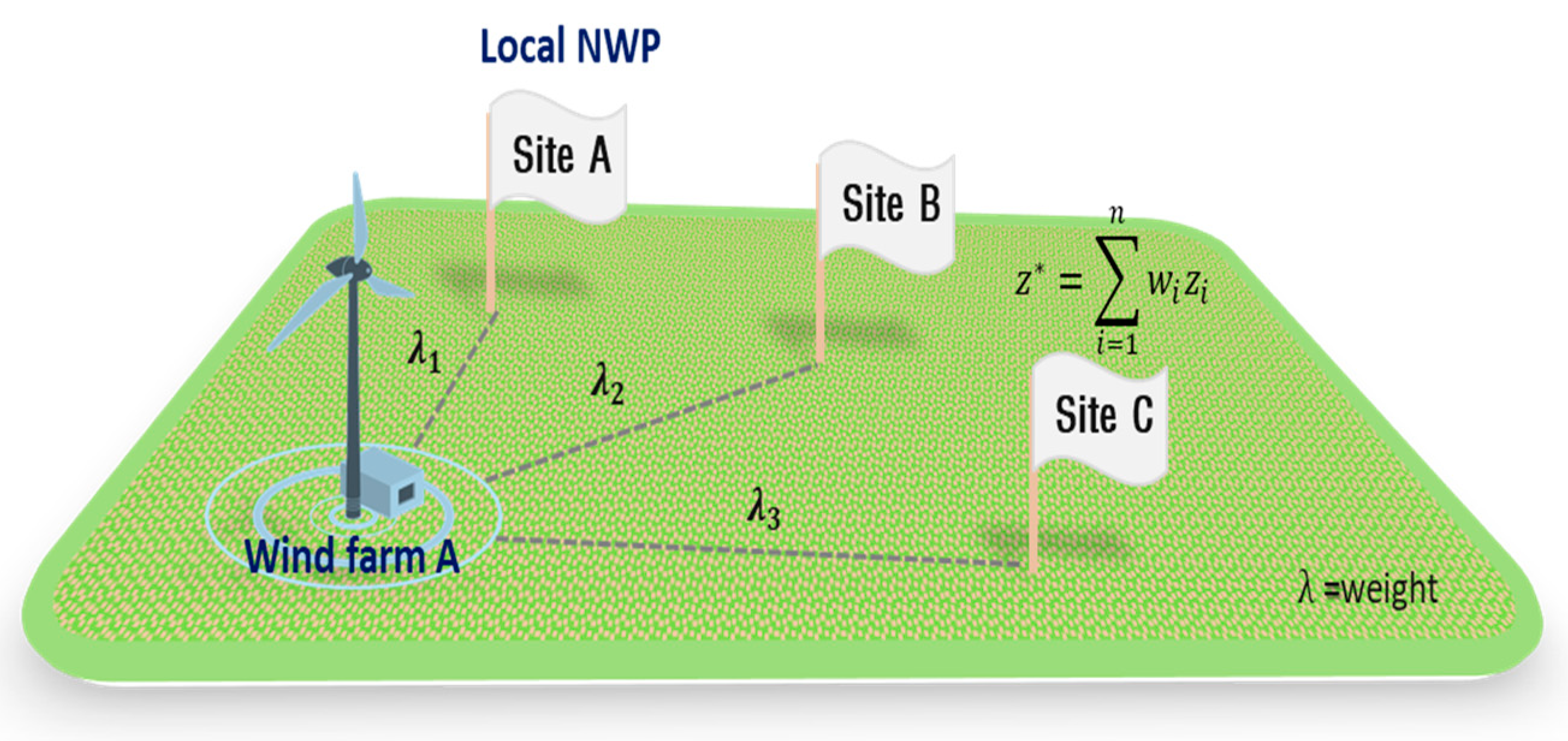
The purpose of spatial modeling is to improve the accuracy of the wind-speed data used as input data in the forecasting model. The wind-speed forecast data used for forecasting were obtained from points near wind farms employed in the local NWP model, which significantly impacts the forecast accuracy. In this study, the spatial limitations of the existing data were supplemented using a spatial modeling referred to as the Kriging technique. This technique is a representative geostatistics technique that uses spatial correlation based on the distance between data to estimate the characteristic value of points of interest. In the case of wind [17,18], spatial correlation exists because similar values occur within the same time-space. Kriging exploits the similarities in the characteristics between two adjacent points in a given space, and is, hence, a suitable technique for interpolating weather variable data [19]. Figure 2 illustrates the concept of the Kriging technique.
Different variants of the Kriging technique can be applied, depending on the weighting method, but the Ordinary Kriging (i.e., the most representative Kriging technique) was employed in this work. The governing equation of the Ordinary Kriging technique is given as follows [20]:
where, denotes a characteristic value at among n points and the weight value is assigned to the spatial data for deriving the characteristic value at the point of interest. The weights were calculated based on a variogram and covariance representing the data’s spatial correlation, and the sum is 1 to avoid bias.
2.2. The ARIMAX Model
ARIMAX is the general ARIMA model with the addition of an exogenous variable (X) [21,22,23]. This model uses the historical data of wind power output as the main variable and wind speed estimated by spatial modeling as the exogenous variable. The general ARIMAX model is defined in Equation (3).
where, , p, , , q, , , , and represent the wind power output at time t, maximum number of time lags, output lagged by time step , coefficient of , maximum number of time lags, coefficient of , white noise, coefficient of , and wind speed at time t, respectively. p and q indicate the order of AR and moving average (MA), which selects the optimal parameter for the minimum Akaike Information Criteria (AIC) [24]. The parameter of minimizing this estimator is important for model identification because it reduces the mean square error, which is an estimate of the variance of the white noise process, and considers the principle of parsimony.
2.3. The SVR Model
SVM is one of the most popular approaches to the field of machine learning, and is used for data classification, data mining, and statistical analysis [25]. SVM determines where new data belongs by optimizing binary classification problems to determine the maximum margin for hyperplane separation. SVR is a model for deriving a regression function by applying SVM. A general regression function can be expressed as and the SVR maps to a high-dimensional feature space to solve nonlinear regression problems. is training data, where x is wind speed and y is wind power output. is the target value, which means the predicted value of wind power output derived through the SVR. The SVR optimization problem is formally defined in Equation (4).
where is the input vector and is the output value. is the magnitude of errors that can be neglected, C is a factor for tradeoff between overfitting and underfitting, and is a slack variable [26]. SVR has excellent generalization capability with high accuracy and without computational complexity relying on the dimensionality of the input space [27].
2.4. The MCS-Based Power Curve Model
The easiest way to predict wind power output using wind speed data is to convert wind speed to power through the manufacturer’s power curve [28]. However, the actual relationship between wind speed and the power generated by wind farms is complicated by turbine aging and control factors, limiting the use of the manufacturer’s deterministic power curves. In this paper, MCS was applied to probabilistically model the relationship between wind speed and wind power output. MCS is a technique used to perform decision-making under uncertain circumstances and to model the probability of different outcomes that are not easily predictable due to random variables [29].
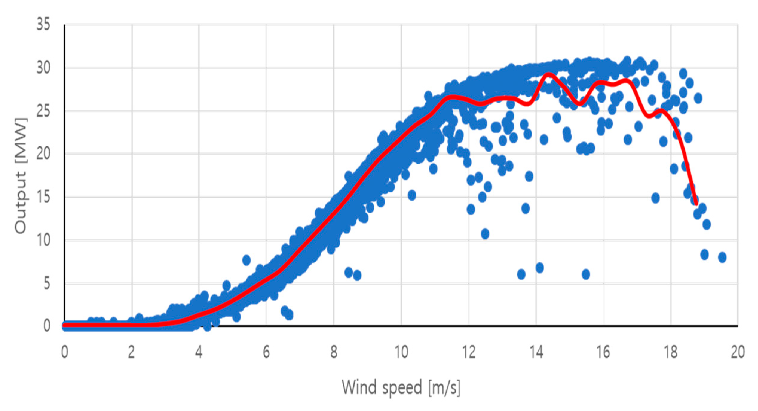
Historical data of wind speed and power output over the past year were used for power curve modeling. After a generation output, database (DB) according to wind speed was modeled, the unit of wind speed was specified in 0.5 m/s to allocate output data corresponding to the interval. Distribution fitting was performed using logistic distribution based on the assigned wind power output. The power curve was then modeled by performing 10,000 random sample extractions through the MCS for a 90% confidence interval of the distribution. Figure 3 shows the power curve estimated by MCS, which reflects the relationship between actual wind speed and power output.
2.5. Forecast Combination
In this paper, we applied the constrained least squares (CLS) regression method to combine the forecast results of the three forecasting models described above. The CLS approach minimizes the sum of squared error in Equation (6) by training a portion of the forecast results [30]. A regression model was used to impose restrictions on the weights of an individual model [31].
where is the forecast obtained from model of n forecasting models and w is the weight. denotes the constant term that is provided if the individual forecasts are biased, and represents the combined forecast.
2.6. Forecasting Performance Evaluation
To assess the model quantitatively, two kinds of error indexes, normalized mean absolute error (NMAE) and root mean square error (RMSE), were used as metrics of forecasting accuracy. Equations (8) and (9) represent the two metrics.
where is the number of forecasting periods, is the measured value at time t, is the forecast value at the same time, and P is the installed capacity of the wind farm.
3. Wind Power Forecasting Case Study
This section details a case study which was conducted for wind farm A with a capacity of 30 MW located in Jeju Island to evaluate wind power output forecasting performance. The NWP model estimates the wind speed for 24 h at 1 h intervals, and the measured data used was supervisory control and data acquisition (SCADA) data measured every hour. Time lags based on electrical power outputs in MW from the SCADA system are attributed to statistical learning for historical values. To compare the performance of a single model and an ensemble model, three single models were used to perform day-ahead forecasting in July and August 2018. The forecast results were generated for 24 h with 1 h intervals. Based on the forecast results in July, we combined the forecast results of the three models through training to produce an ensemble result for August. Figure 4 shows the training and evaluation periods for the forecast, using data from the past 28 days for the day-ahead forecast.
3.1. Spatial Modeling Results for Wind Speed Correction
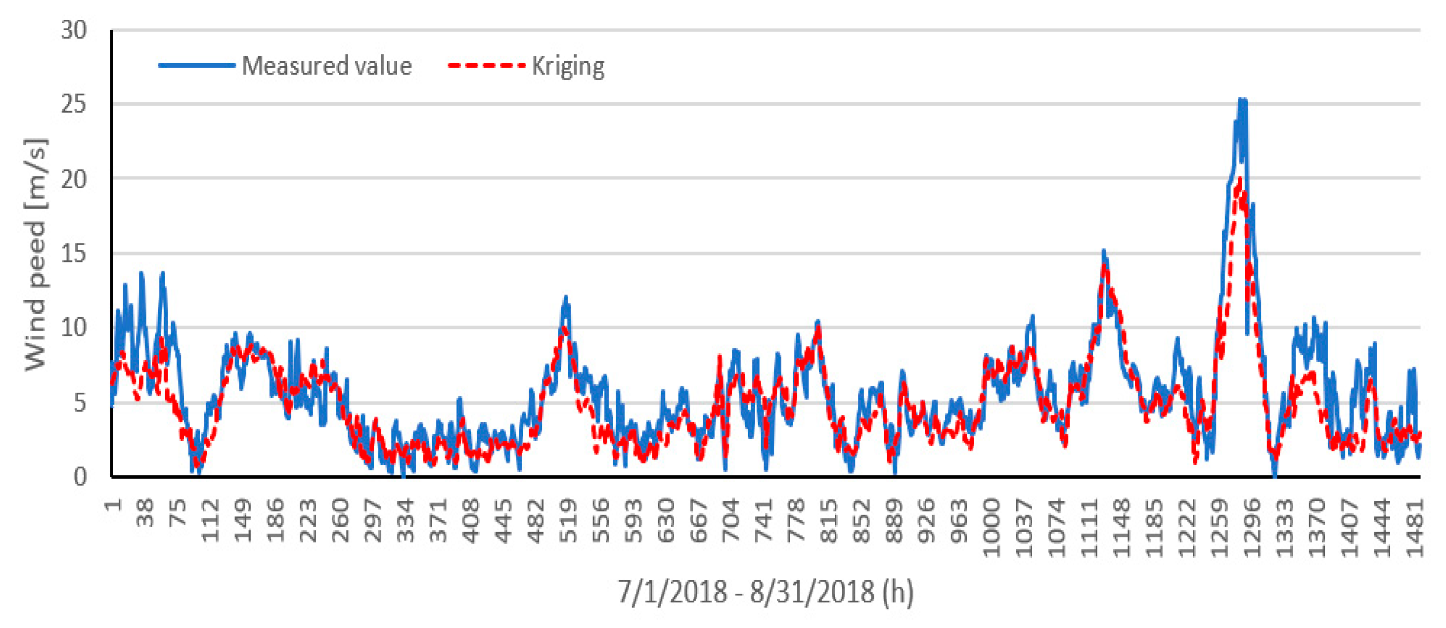
In order to perform the forecast, wind speed forecast values were required for the forecast period. In this paper, the forecast value of the point near the wind farm was obtained from the local NWP model and corrected through spatial modeling. NWP data of 20 points were used, and the wind speed at the wind farm was estimated using Ordinary Kriging—a spatial modeling technique. Figure 5 shows the wind speed estimates for the forecast period. The red dashed line represents the estimated wind speed, with an overall RMSE of 1.76 m/s. The data were used as the input data for the wind power output forecast models.
3.2. Wind Power Output Forecasting Results Using Ensemble Model
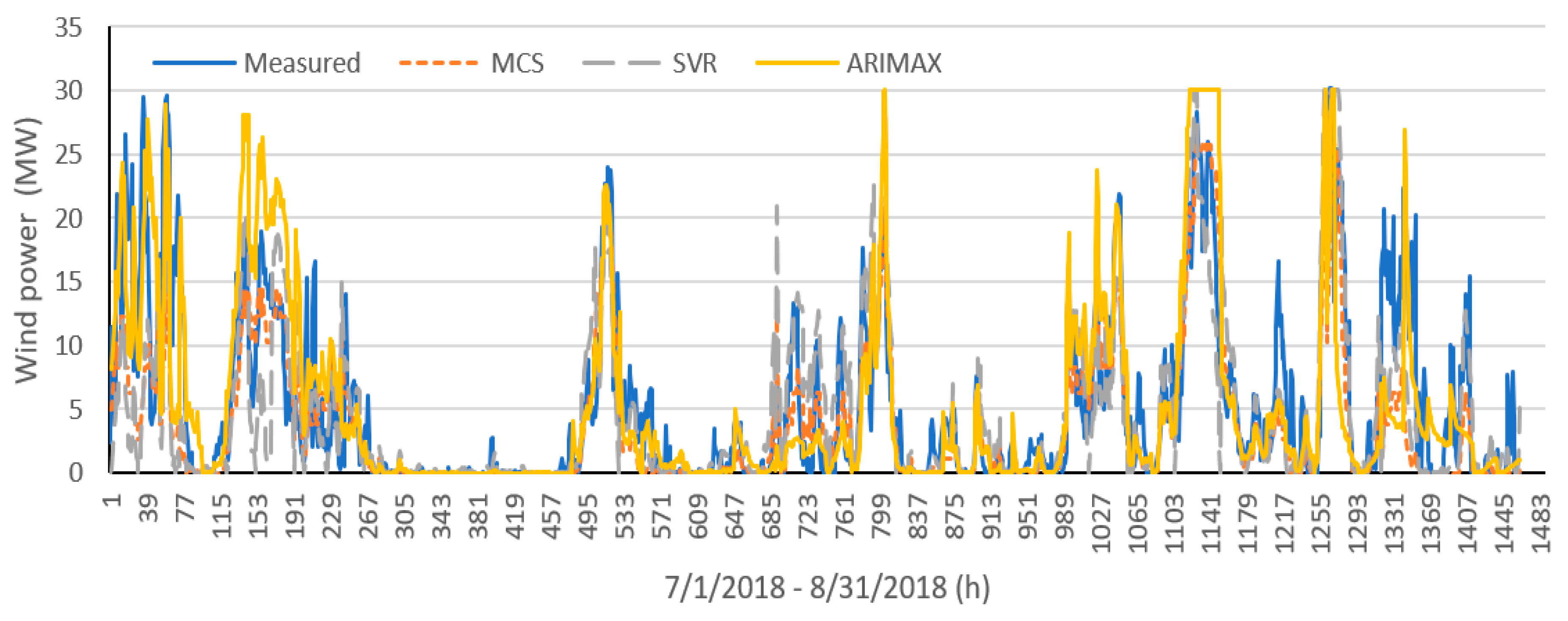
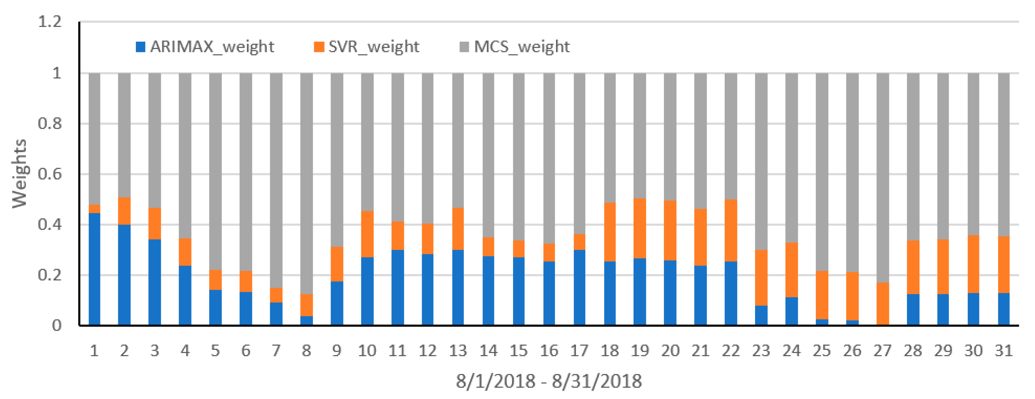
We performed the wind power output forecasting in July and August using single models. Figure 6 shows the forecast values of the single models for these two months. The accuracy of the forecast output values for each model is shown in Table 3. In both months, the accuracy of the MCS-based power curve model is high, but because this model is significantly affected by wind speed prediction results, an ensemble approach is needed to prevent bias of the results. In order to perform the ensemble forecasting for August by combining the single forecasting results, the weights were calculated through CLS regression based on the previous 28 days’ forecasting results. The weighting results are shown in Figure 7.
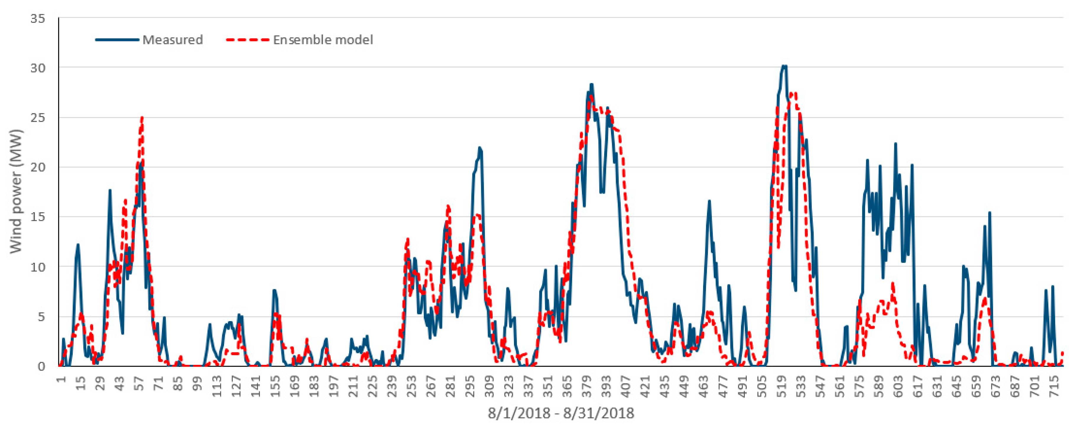
Figure 8 shows the results of combining the forecasting results by applying the weights in Figure 7. The forecasting error is shown in Table 4. Accuracy is improved through the ensemble approach. The ensemble approach does not always improve accuracy, but it can compensate for overshoots occurring at turning points and prevent bias of the results. Thus, the ensemble approach is a viable alternative for improving the forecasting model in that its results are often more accurate than single forecasting results.
4. Conclusions
Intermittent power fluctuation depending on the wind climate is the biggest challenge in integrating wind into the grid. Therefore, a wind power forecasting technique is essential for reliable grid operation and integration. In this paper, we proposed a short-term wind power forecasting model that combined three statistical methods. Wind speed prediction data were obtained from the local NWP model and corrected for the wind speed in a wind farm through the Kriging technique, a spatial modeling technique that uses the spatial correlation for wind speeds to increase the accuracy of NWP models.
In order to verify the proposed method, a case study was performed using empirical data from a wind farm on Jeju Island. Two months’ worth of day-ahead predictions using three single models showed that the MCS-based power curve model performed best. However, this method requires a great deal of historical data for power curve modeling, and it is difficult to obtain relatively accurate results when the NWP model’s prediction accuracy is low. By combining single forecasting results based on the ensemble technique, we found that the prediction accuracy was improved. While the ensemble model did not have good performance over all time periods, combining multiple single models prevented bias in the forecasting results. These practical forecasts allow the grid operator to know the expected wind power output at a specific time, enabling stable grid operation.
In the future, we will apply Random Forest (RF) to a proposed model in order to enhance the forecasting error and perform forecast for various regions. Further, wind direction will be considered to spatial modeling and application when wind direction data is available from the Korean NWP system.
Author Contributions
J.H. conceived and designed the overall research; Y.K. implemented each forecasting model and conducted the experimental simulation; J.H. and Y.K. wrote the paper; and J.H. guided the research direction and supervised the entire research process. All authors have read and agreed to the published version of the manuscript.
Funding
This research received no external funding.
Acknowledgments
This work was supported by the Korea Electric Power Corporation (No.R18XA06-55).
Conflicts of Interest
The authors declare no conflict of interest.
Abbreviations
| List of Symbols and Abbreviations: | |||
| NWP | Numerical weather prediction | ARIMAX | Autoregressive integrated moving average with exogenous variable |
| AR | Autoregressive | ||
| ARMA | Autoregressive moving average | SVR | Support vector machine |
| ARIMA | Autoregressive integrated moving average | MCS | Monte-Carlo simulation |
| BP | Back propagation | ||
| ANN | Artificial neural network | RBF | Radial basis function |
| SVM | Support vector machine | MA | Moving average |
| AI | Artificial intelligence | AIC | Akaike information criteria |
| ML | Machine learning | CLS | Constrained least squares |
| NMAE | Normalized mean absolute error | RMSE | Root mean square error |
| DB | Database | SCADA | Supervisory control and data acquisition |
References
- Renewable Energy Policy Network for the 21st Century. Renewable 2019 Global Status Report; REN21: Paris, France, 2019; ISBN 978-3-9818911-7-1. [Google Scholar]
- Global Wind Energy Council. Global Wind Energy Outlook; GWEC: Sydney, Australia, 2016. [Google Scholar]
- Soman, S.S.; Zareipour, H.; Malik, O.; Mandal, P. A review of wind power and wind speed forecasting methods with different time horizons. N. Am. Power Symp. 2010, 2010, 1–8. [Google Scholar] [CrossRef]
- Lund, H. Large-scale integration of wind power into different energy systems. Energy 2005, 30, 2402–2412. [Google Scholar] [CrossRef]
- Riahy, G.H.; Abedi, M. Short term wind speed forecasting for wind turbine applications using linear prediction method. Renew. Energy 2008, 33, 35–41. [Google Scholar] [CrossRef]
- Barbosa de Alencar, D.; De Mattos Affonso, C.; Limão de Oliveira, R.C.; Moya Rodríguez, J.L.; Leite, J.C.; Reston Filho, J.C. Different Models for Forecasting Wind Power Generation: Case Study. Energies 2017, 10, 1976. [Google Scholar] [CrossRef] [Green Version]
- Foley, A.M.; Leahy, P.G.; Marvuglia, A.; Mckeogh, S.J. Current methods and advances in forecasting of wind power generated power. Renew. Energy 2012, 37, 1–8. [Google Scholar] [CrossRef] [Green Version]
- Chang, W.Y. A literature review of wind forecasting methods. J. Power Energy Eng. 2014, 2, 161–168. [Google Scholar] [CrossRef]
- Wang, X.; Guo, P.; Huang, X. A review of wind power forecasting models. Energy Procedia 2011, 12, 770–778. [Google Scholar] [CrossRef] [Green Version]
- Shokrzadeh, S.; Jozani, M.; Bibeau, E. Wind turbine power curve modeling using advanced parametric and nonparametric methods. IEEE Trans. Sustain. Energy 2014, 5, 1262–1269. [Google Scholar] [CrossRef]
- Lei, M.; Shiyan, L.; Chuanwen, J.; Hognling, L.; Yan, Z. A review on the forecasting of wind speed and generated power. Renew. Sustain. Energy Rev. 2009, 13, 915–920. [Google Scholar] [CrossRef]
- Wang, Y.; Hu, Q.; Meng, D.; Zhu, P. Deterministic and probabilistic wind power forecasting using a variational Bayesian-based adaptive robust multi-kernel regression model. Appl. Energy 2017, 208, 1097–1112. [Google Scholar] [CrossRef]
- Shi, J.; Guo, J.; Zheng, S. Evaluation of hybrid forecasting approaches for wind speed and power generation time series. Renew. Sustain. Energy Rev. 2012, 16, 3471–3480. [Google Scholar] [CrossRef]
- Sideratos, G.; Hatziargyriou, N.D. An advanced statistical method for wind power forecasting. IEEE Trans. Power Syst. 2007, 22, 258–265. [Google Scholar] [CrossRef]
- Monteiro, C.; Bessa, R.; Miranda, V.; Botterud, A.; Wang, J.; Conzelmann, G. Wind Power Forecasting: State-of-the-Art 2009; Technical Report No. ANL/DIS-10-1; Argonne National Lab (ANL): Argonne, IL, USA, 2009.
- Zhao, X.; Wang, S.; Li, T. Review of evaluation criteria and main methods of wind power forecasting. Energy Procedia 2011, 12, 761–769. [Google Scholar] [CrossRef] [Green Version]
- Li, J.; Heap, A.D. A Review of Spatial Interpolation Methods for Environmental Scientist; Geoscience Australia: Canberra, Australia, 2008; pp. 1448–2177.
- Cressie, N. Statistics for Spatial Data; Wiley: New York, NY, USA, 1993; ISBN 9780471002550. [Google Scholar]
- Luo, W.; Taylor, M.C.; Parker, S.R. A comparison of spatial interpolation methods to estimate continuous wind speed surfaces using irregularly distributed data from England and Wales. Int. J. Climatol. 2008, 28, 947–959. [Google Scholar] [CrossRef]
- Amjady, N.; Abedinia, O. Short term wind power prediction based on improved Kriging interpolation, empirical mode decomposition, and closed-loop forecasting engine. Sustainability 2017, 9, 2104. [Google Scholar] [CrossRef] [Green Version]
- Peter, Ď.; Silvia, P. ARIMA vs. ARIMAX-which approach is better to analyze and forecast macroeconomic time series. In Proceedings of the 30th International Conference Mathematical Methods in Economics, Karviná, Czech Republic, 1–13 September 2012. [Google Scholar]
- Box, G.E.; Jenkins, G.M.; Reinsel, G.C.; Ljung, G.M. Time Series Analysis: Forecasting and Control; John Wiley & Sons: Hoboken, NJ, USA, 2016; ISBN 978-1-118-67502-1. [Google Scholar]
- Kim, D.; Hur, J. Short-term probabilistic forecasting of wind energy resources using the enhanced ensemble method. Energy 2018, 157, 211–226. [Google Scholar] [CrossRef]
- Brockwell, P.J.; Davis, R.A. Introduction to Time Series and Forecasting, 2nd ed.; Springer: New York, NY, USA, 2002. [Google Scholar]
- Law, M. A Simple Introduction to Support Vector Machines. Available online: https://sikoried.github.io/sequence-learning/09-sequence-kernels/intro_svm_new.pdf (accessed on 27 January 2020).
- Drucker, H.; Burges, C.J.; Kaufman, L.; Smola, A.J.; Vapnik, V. Support vector regression machines. In Advanced in Neural Information Processing Systems; The MIT Press: Cambridge, MA, USA, 1997; pp. 155–161. [Google Scholar]
- Award, M.; Khanna, R. Efficient Learning Machines: Theories, Concepts, and Applications for Engineers and System Designers; Springer: Berlin, Germany, 2015; ISBN 978-1-4302-5990-9. [Google Scholar]
- Wu, Y.K.; Hong, J.S. A literature review of wind forecasting technology in the world. In Proceedings of the 2007 IEEE Lausanne Power Tech, Lausanne, Switzerland, 1–5 July 2007. [Google Scholar] [CrossRef]
- Rubinstein, R.Y.; Kroese, D.P. Simulation and the Monte Carlo Method, 3rd ed.; John Wiley & Sons: Hoboken, NJ, USA, 2017; ISBN 978-1-118-63216-1. [Google Scholar]
- Weiss, C.E.; Raviv, E.; Roetzer, G. Forecast Combination in R using Forecast Comb Package. R. J. 2018, 10. [Google Scholar] [CrossRef] [Green Version]
- Thordarson, F.Ö.; Madsen, H.; Nielsen, H.A.; Pinson, P. Conditional weighted combination of wind power forecasts. Wind Energy 2010, 13, 751–763. [Google Scholar] [CrossRef]
Figure 1.
The proposed algorithm for wind power forecasting.

Figure 2.
The concept of the Kriging technique.

Figure 3.
Power curve estimated by MCS (the red line is estimated power curve and the blue dots are observed power).
Figure 3.
Power curve estimated by MCS (the red line is estimated power curve and the blue dots are observed power).

Figure 4.
Training and evaluation periods for forecast.

Figure 5.
Spatial modeling results (the x axis represents the 1 h intervals of time for the estimated period).
Figure 5.
Spatial modeling results (the x axis represents the 1 h intervals of time for the estimated period).

Figure 6.
Forecast results of single models results (the x axis represents the 1 h intervals time for the forecast period).
Figure 6.
Forecast results of single models results (the x axis represents the 1 h intervals time for the forecast period).

Figure 7.
Weights for ensemble model (the x axis represents the 1 day intervals time for the evaluation period).
Figure 7.
Weights for ensemble model (the x axis represents the 1 day intervals time for the evaluation period).

Figure 8.
Forecast results of ensemble model (the x axis represents the 1 h intervals time for the evaluation period).
Figure 8.
Forecast results of ensemble model (the x axis represents the 1 h intervals time for the evaluation period).


Table 1.
Classification of wind power forecasting methods.
| Forecasting Methods | Models | Examples | Remarks |
|---|---|---|---|
| Physical models | NWP |
|
|
| Statistical models | Time series model |
|
|
| AI model |
|
| |
| ML model |
|
| |
| Combination models | - |
|
|
Table 2.
Classification of time horizons for wind power forecasting.
| Time Horizon | Time | Application Purpose |
|---|---|---|
| Very-short-term | 8 h ahead |
|
| Short-term | Up to 48 h ahead |
|
| Medium-term | Up to 7 days ahead |
|
| Long-term | 1 year of more ahead |
|
Table 3.
Accuracy of single models for two months.
| Model | ARIMAX | SVR | MCS |
|---|---|---|---|
| NMAE | 9.81 | 10.43 | 8.48 |
| RMSE | 4.87 | 5.22 | 4.44 |
Table 4.
Accuracy of wind power forecast.
| Model | ARIMAX | SVR | MCS | Ensemble |
|---|---|---|---|---|
| NMAE | 10.39 | 9.44 | 9.07 | 8.75 |
| RMSE | 5.01 | 4.34 | 4.35 | 4.28 |
© 2020 by the authors. Licensee MDPI, Basel, Switzerland. This article is an open access article distributed under the terms and conditions of the Creative Commons Attribution (CC BY) license (http://creativecommons.org/licenses/by/4.0/).
Share and Cite
MDPI and ACS Style
Kim, Y.; Hur, J. An Ensemble Forecasting Model of Wind Power Outputs Based on Improved Statistical Approaches. Energies 2020, 13, 1071. https://doi.org/10.3390/en13051071
AMA Style
Kim Y, Hur J. An Ensemble Forecasting Model of Wind Power Outputs Based on Improved Statistical Approaches. Energies. 2020; 13(5):1071. https://doi.org/10.3390/en13051071
Chicago/Turabian StyleKim, Yeojin, and Jin Hur. 2020. "An Ensemble Forecasting Model of Wind Power Outputs Based on Improved Statistical Approaches" Energies 13, no. 5: 1071. https://doi.org/10.3390/en13051071
Note that from the first issue of 2016, this journal uses article numbers instead of page numbers. See further details here.