Autocorrelation Ensemble Average of Larger Amplitude Impact Transients for the Fault Diagnosis of Rolling Element Bearings

Abstract

Rolling element bearings are one of the critical elements in rotating machinery of energy engineering systems. A defective roller of bearing moves in and out of the load zone during each revolution of the cage. Larger amplitude impact transients (LAITs) are produced when the defective roller passes the load zone centre and the defective area strikes the inner or outer races. A series of LAIT segments with higher signal to noise ratio are separated from a continuous vibration signal according to the bearing geometry and kinematics. In order to eliminate the phase errors between different LAIT segments that can arise from rotational speed fluctuations and roller slippages, unbiased autocorrelation is introduced to align the phases of LAIT segments. The unbiased autocorrelation signals make the ensemble averaging more accurate, and hence, archive enhanced diagnostic signatures, which are denoted as LAIT-AEAs for brevity. The diagnostic method based on LAIT separation and autocorrelation ensemble average (AEA) is evaluated with the datasets captured from real bearings of two different experiment benches. The validation results of the LAIT-AEAs are compared with the squared envelope spectrums (SESs) yielded based on two state-of-the-art techniques of Fast Kurtogram and Autogram.

1. Introduction

Rotating machines, such as turbines, motors and mechanical transmission systems, play an important role in many energy generation or consumption systems. Fault diagnosis of rotating machinery, which supports maintenance and then helps to prevent the machines from malfunctions, failures or even fatal accidents, is of vital importance for guaranteeing the efficiency and reliability of engineering systems. Rolling element bearings are one of the critical elements in rotating machinery and bearing faults are often the causes for unexpected breakdown of rotating machinery. Thus, fault diagnosis of rolling element bearings has received a lot of attention [1].

When a localised defect on the outer or inner race of rolling element bearings is struck by the rollers or a localised defect on a roller strikes the inner and outer races, high-frequency resonances are excited on system structures, which lead to vibration responses of successive impact transients. The vibration signal produced by localised defect is recognised as the modulation between the low frequency fault components and high-frequency resonances [2,3]. Most techniques for fault diagnosis of rolling element bearings are based on envelope analysis [4,5,6], i.e., the diagnostic information is firstly enhanced by filtering the modulated signal in the high resonance frequency bands; then, the modulated signal is demodulated to yield the envelope signal, and the fault frequency components are investigated in envelope spectrums.

Finding an optimal resonance frequency band for filtering and demodulation has been a research focus for a long time as it is critical for the success of envelope analysis methods. In recent years a number of successful tools, such as Fast Kurtogram [7], Protrugram [8] and Autogram [9], have been developed for finding the optimal frequency band. The Fast Kurtogram finds the optimal band according to the kurtosis of the filtered time signal in different filter banks. The Protrugram employs the kurtosis of the envelope spectrums in different fixed demodulation bandwidth. While the Autogram employs the unbiased autocorrelation of the squared envelope of different frequency band nodes. These tools are very effective for most situations to give an optimal band. However, they have little mechanisms of noise suppression [10]. In addition, because of the searching operation for different bands, their computation costs are generally high and limited for online applications.

Another challenge for fault diagnosis of rolling element bearings is the low signal to noise ratio (SNR), which is common in industrial applications. The transients generated by bearing defects can be polluted by random noise as well as harmonics excited by other elements such as shafts, gears, motors, compressors, belts, propellers, pistons, and so on. Thus research efforts are also focused on signal preprocessing methods used for improving the SNR. Time synchronous averaging (TSA) is one of the most powerful preprocessing methods for enhanced fault diagnosis of rotating machinery [11,12]. The philosophy of TSA is simple: TSA extracts particular periodic signals from a composite signal by averaging divided segments; each segment corresponds to one period of the synchronising signal; thus, periodic components synchronous with this period are enhanced, and any other periodic components as well as random noise converge asymptotically towards zero. As the characteristic frequency of a gearbox is typically Z multiples of the shaft rotational frequency where Z is the number of the gear teeth, the characteristic frequency harmonics of the gearbox can be synchronised with the shaft frequency and TSA is successfully used for achieving enhanced fault diagnosis of gearboxes [13,14,15,16].

However, applying TSA to fault diagnosis of rolling element bearings can encounter a number of challenges. The fault frequencies of rolling element bearings are usually not exactly integer multiples of shaft frequency; thus, shaft speed cannot be used as trigger for performing TSA. Moreover, speed fluctuations and roller slippages cause phase errors of divided signal segments, leading to great loss of diagnostic information due to the inaccurate ensemble averaging of the non-synchronous segments. Nevertheless, efforts are made for improving TSA to bearing fault diagnosis. Siegel et al. [17] generated a trigger signal from the outer race fault frequency and proposed a tachometer-less synchronously averaged envelope method. The method further enhanced the fault signatures of outer race defects which can also be detected with classical envelope analysis. McFadden and Toozhy [18] applied a modified synchronous averaging method for diagnosing the inner race defect of rolling element bearings. As the ball pass frequency of inner race $f_{\mathrm{BPI}}$, the shaft frequency $f_{\mathrm{r}}$ and the cage frequency $f_{\mathrm{c}}$ satisfy the equation $f_{\mathrm{BPI}}=Z\left(f_{\mathrm{r}}-f_{\mathrm{c}}\right)$, the fault frequency of $f_{\mathrm{BPI}}$, which consists of integer multiples of $\left(f_{\mathrm{r}}-f_{\mathrm{c}}\right)$, can be enhanced by synchronising with the shaft frequency relative to the cage frequency. The major drawback of the modified synchronous averaging method is that measuring the cage frequency is not allowed in most industrial applications.

It is worth noting that transients of different intensities are generated by the defects of moving parts, i.e., the rollers and inner race. The moving parts move in and out of the load zone during rotation. Larger amplitude impact transients (LAITs) are produced when a defective moving part gets closer to the load zone centre and undertakes heavier load. On the contrary, smaller amplitude impact transients (non-LAITs) are produced when the defective part is out of the load zone. This is also the reason why modulation sidebands of shaft frequency appear around the fault frequency of inner race and sidebands of cage frequency appear around the fault frequency of rollers [19,20]. The LAIT segments have more significant amplitudes and thus more reliable and accurate diagnostic results can be produced when just the LAIT segments are selected for fault diagnosis. In comparison, both the LAIT and non-LAIT segments are involved in conventional envelope analysis and TSA based methods. It has been shown by the authors [21] that the LAIT separation along with bandpass filtering, demodulation and low-pass filtering gives a signature of envelope ensemble average. Moreover, the signature is sensitive to defect, while robust to rotational speed fluctuations and roller slippages. However, yielding the envelope ensemble average signatures needs the same effort of finding an optimal resonance frequency band, which is still an open challenge.

Autocorrelation can be used to enhance the harmonic components by eliminating interfering impulses and white noise [22]. Moreover, as the autocorrelation signals of harmonic components have an initial phase of 0, the autocorrelation signals of the LAIT segments share the same initial phase. Thus, the autocorrelation can be used to align the LAIT segments and thereby overcome the effect of phase errors concerned in the bearing transients. This paper presents a new method based on the LAIT separation and autocorrelation ensemble averaging to overcome the challenges of finding optimal resonance frequency band and improving the SNR of defective bearing signals. The paper is organised as follows. Section 2 presents the theoretical background of the autocorrelation ensemble averaging of LAIT segments first, and then introduces the flowchart of the proposed diagnostic method. In Section 3, the proposed method is validated with both experimental signals captured from a test bench of machinery fault simulation and datasets provided by the Case Western Reserve University Bearing Data Center. The validation results are compared with the squared envelope spectrums (SESs) obtained based on Fast Kurtogram and Autogram to examine the merits of the proposed method. Finally, the conclusions are drawn in Section 4.

2. Methodology

2.1. Autocorrelation Ensemble Averaging of LAIT Segments

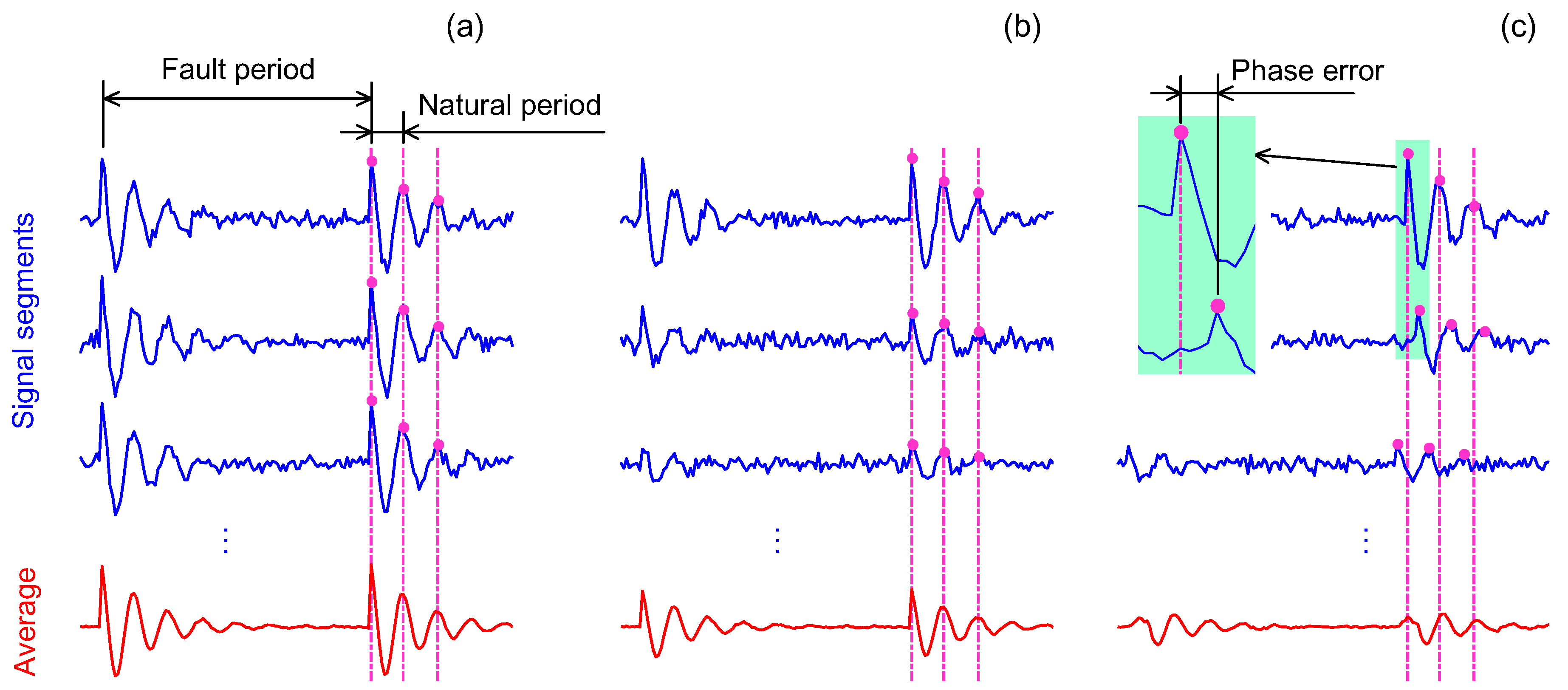
Rollers of bearings are moving parts and their position to the load zone is always changing during operation. A defective roller moving in and out of the load zone causes amplitude modulation of vibration signals. The roller is more heavily loaded when it gets closer to the load zone centre. Thus, LAITs can be generated when the defective roller approaches the load zone centre. On the contrary, non-LAITs can be generated when the defective roller departs from the load zone centre. The averaging result of the LAIT segments only, as shown in Figure 1a, has larger transient amplitudes, compared with the averaging result of both the LAIT and non-LAIT segments, as shown in Figure 1b. Thus, separating the LAIT segments for each roller can help to achieve more reliable and accurate diagnostic results.

A LAIT separation method, the details of which are in Reference [21], was developed by the authors. The method denotes the first roller that will pass the load zone centre as RE 1, and denotes the following rollers that will pass the load zone centre successively after RE 1 as RE 2, RE 3, …, and RE Z, where Z is the number of the rollers. For a defective roller of RE i, the method divides a vibration signal into successive spins. There is just one spin occurring across the load zone centre for each revolution of the cage. This spin is denoted as the LAIT spin. The LAIT spins are separated from the successive spins according to the condition of:

$$T_{\mathrm{c}}-T_{\mathrm{BS}}<\mathrm{mod}\left(t_{i,j},T_{\mathrm{c}}\right)\le T_{\mathrm{c}}$$

(1)

where $t_{i,j}$ is the time phase of the jth spin of RE i; $T_{\mathrm{c}}$ is the revolution period of the cage; $T_{\mathrm{BS}}$ is the ball spin period. The vibration segments that centre on the LAIT spins are denoted as LAIT segments for convenience.

The separated LAIT segments are not rigorously synchronous as speed fluctuations as well as roller slippages happen inevitably, and both of them can cause phase errors [20,21]. Ensemble averaging of the separated LAIT segments with phase errors can cause great loss of diagnostic information. Typically, the impact transients caused by defects have a waveform of damping oscillation, which lasts several periods of the natural resonance frequency as shown in Figure 1a. Phase errors in the time scale of 1/4 natural frequency period can cause great information loss, as shown in Figure 1c. In addition, the natural frequency period is typically smaller than 0.001 s as the natural frequency of a bearing is as high as several thousand Hz. Thus, phase errors of 2.5 × 10⁻⁴ s are not negligible.

To overcome the problem of phase errors, the separated LAIT segments are firstly demodulated to yield the envelopes of the transients, and then, autocorrelation is introduced to align the LAIT envelopes. The interesting components in the LAIT envelopes are the harmonics of the roller spin frequency $f_{\mathrm{BS}}$ and the roller fault frequency $f_{\mathrm{BF}}$. As two transients can be generated during a spin period by a defective roller, thus $f_{\mathrm{BF}}=2f_{\mathrm{BS}}$. The LAIT envelopes of a defective roller can be presented as:

$$v\left(t\right)={{\displaystyle \sum }}_n{x}_n\left(t\right)+h\left(t\right)+g\left(t\right)$$

(2)

where $x_n\left(t\right)$ denotes the nth order harmonic of the fault frequency, $h\left(t\right)$ denotes the interfering harmonics excited by other rotating parts, $g\left(t\right)$ denotes the background white noise. The nth order harmonic of the fault frequency can be presented as:

$$x_n\left(t\right)=A_n\sin \left({\omega }_{n}t+{\phi }_n\right)$$

(3)

where $A_n$ is the amplitude, ${\omega }_n=2\mathsf{\pi }n{f}_{\mathrm{BF}}$ is the nth order angular frequency, and ${\phi }_n$ is the initial phase. The autocorrelation of the harmonic can be presented as:

$$R_x^n\left(\tau \right)=\frac{1}{T}{{\displaystyle \int }}_0^T{A}_n\sin \left({\omega }_{n}t+{\phi }_n\right)A_n\sin \left[{\omega }_n\left(t+\tau \right)+{\phi }_n\right]\mathrm{d}t$$

(4)

where $\tau$ is the time-lag. By presenting the integration interval as $T=2\mathsf{\pi }/{\omega }_n$ and the phase as $\left({\omega }_{n}t+{\phi }_n\right)=\theta$, the autocorrelation can be presented as:

$$R_x^n\left(\tau \right)=\frac{A_n^2}{2\mathsf{\pi }}{{\displaystyle \int }}_0^{2\mathsf{\pi }}\sin \left(\theta \right)\sin \left(\theta +{\omega }_n\tau \right)\mathrm{d}\theta =\frac{A_n^2}{2}\cos {\omega }_n\tau$$

(5)

It can be seen that the autocorrelation of a periodic signal is periodic with the same period of $2\mathsf{\pi }/{\omega }_n$ and keeps the amplitude information of $A_n$. Moreover, the autocorrelation has an initial phase of 0. It means that all autocorrelation signals of the LAIT envelopes are of 0 initial phase, i.e., they are aligned with each other. Thus, the autocorrelations of the LAIT envelopes can overcome the effect of phase errors concerned in the bearing transients and make the ensemble averaging more effective.

In addition, the autocorrelation can also be used to eliminate interfering impulses and white noise. As $x_n\left(t\right)$, $h\left(t\right)$ and $g\left(t\right)$ are independent from each other, the autocorrelation of $v\left(t\right)$ can be expressed as:

$$R_v\left(\tau \right)={{\displaystyle \sum }}_n\frac{A_n^2}{2}\cos {\omega }_n\tau +R_h\left(\tau \right)+R_g\left(\tau \right)$$

(6)

where $R_h\left(\tau \right)$ and $R_g\left(\tau \right)$ are the autocorrelation of $h\left(t\right)$ and $g\left(t\right)$, respectively.

As the autocorrelation of white noise is an impulse function, which have a strong peak at $\tau =0$ and is negligible for all other time lags, i.e., $R_g\left(\tau >0\right)\approx 0$. The autocorrelation of the signal is mainly contributed with the autocorrelation of periodic transients. As $R_h\left(\tau =m{T}_{\mathrm{BF}}\right)\approx 0$ if the frequency of $h\left(t\right)$ is far away from the fault frequency, where $T_{\mathrm{BF}}=1/f_{\mathrm{BF}}$ is the roller fault period, the autocorrelation value at the time-lags of the fault period can be presented as:

$$R_v\left(\tau =m{T}_{\mathrm{BF}}\right)\approx {{\displaystyle \sum }}_n\frac{A_n^2}{2}\cos \left(2\mathsf{\pi }n{f}_{\mathrm{BF}}·m{T}_{\mathrm{BF}}\right)={{\displaystyle \sum }}_n\frac{A_n^2}{2}$$

(7)

It can be seen from Equation (7) that the fault signatures are enhanced via autocorrelation especially because of the additive effect of high order harmonics.

Based on these two important properties of phase alignment and noise reduction, the autocorrelation is introduced to make the ensemble averaging of the LAIT envelopes more reliable. The unbiased autocorrelation of the kth LAIT envelope for RE i is denoted as:

$$R_{i,k}\left({\tau }_j\right)=\frac{1}{L_2-{\tau }_j{f}_{\mathrm{s}}}{\displaystyle \sum }_{n=1}^{L_2-{\tau }_j{f}_{\mathrm{s}}}{E}_{i,k}\left(t_n\right)E_{i,k}\left(t_n+{\tau }_j\right)=\left[r_{i,k}\left({\tau }_1\right),r_{i,k}\left({\tau }_2\right),r_{i,k}\left({\tau }_3\right),\cdots ,r_{i,k}\left({\tau }_{L_2}\right)\right]$$

(8)

where $E_{i,k}$ is kth LAIT envelope for RE i, $f_{\mathrm{s}}$ is the sampling frequency and $L_2$ is the rounded length of the LAIT segments.

In the former LAIT separation method, the rounded length was set to be $L_2=\left[T_{\mathrm{BS}}{f}_{\mathrm{s}}\right]$, in which $f_{\mathrm{s}}$ is the sampling frequency, i.e., each segment covers only one spin period. As for autocorrelation, the information of the periodic transients can be better extracted if the separated segments are longer to include more transients. To enhance the detection performance, the rounded length is extended to cover the whole load zone:

$$L_2=\left[\frac{\zeta }{2\mathsf{\pi }{f}_{\mathrm{c}}}{f}_{\mathrm{s}}\right]$$

(9)

where $\zeta$ is the subtended angle of the load zone. In this way, the autocorrelation of the LAIT envelope allows the spin period component to be enhanced by combining the effects of multiple spins.

The autocorrelation values at the time-lags of the fault period $T_{\mathrm{BF}}$ and the spin period $T_{\mathrm{BS}}$ correspond to the fault frequency component and the spin frequency component, respectively. To highlight the autocorrelation values at $T_{\mathrm{BF}}$ and $T_{\mathrm{BS}}$, the autocorrelation values only in the time-lag interval of $\left[0.5T_{\mathrm{BF}}, 2.5T_{\mathrm{BF}}\right]$ are kept and investigated.

Finally, the autocorrelation ensemble average (AEA) is yielded for RE i and can be presented as:

$$A_i\left({\tau }_l\right)=\frac{1}{K}{\displaystyle \sum }_{k=1}^K{r}_{i,k}\left({\tau }_l\right),0.5T_{\mathrm{BF}}\le {\tau }_l\le 2.5T_{\mathrm{BF}}$$

(10)

where $K$ is the number of the LAIT segments.

To obtain reliable and comparable results, the linear trend in the AEAs is removed by:

$$A_i^{\prime }\left({\tau }_l\right)=A_i\left({\tau }_l\right)-{\widehat{A}}_i\left({\tau }_l\right),0.5T_{\mathrm{BF}}\le {\tau }_l\le 2.5T_{\mathrm{BF}}$$

(11)

where ${\widehat{A}}_i$ is the least-squares fit of a straight line to $A_i$; then, each detrended AEA is shifted with respect to the local minimum:

$$A_i^{″}\left({\tau }_l\right)=A_i^{\prime }\left({\tau }_l\right)-\underset{l}{\min }{A}_i^{\prime }\left({\tau }_l\right),0.5T_{\mathrm{BF}}\le {\tau }_l\le 2.5T_{\mathrm{BF}}$$

(12)

In this way, $A_i^{″}$ for RE i has a local minimum of 0. The detrended and shifted AEAs are hereafter referred to as LAIT-AEAs for short.

2.2. Diagnostic Schematic Diagram

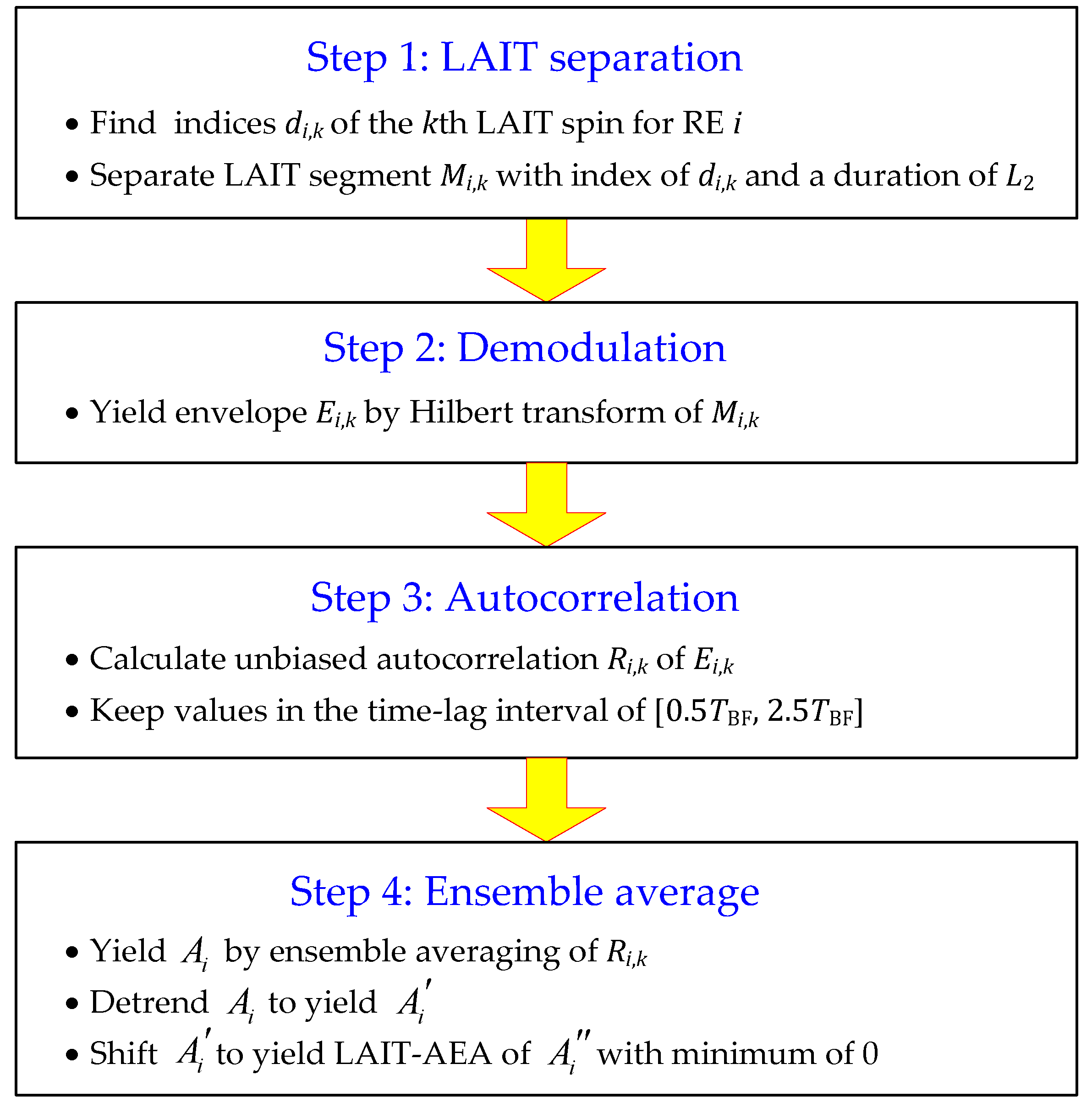
By employing the autocorrelation to align the separated LAITs before ensemble averaging, a fault diagnostic method based on the LAIT separation and autocorrelation ensemble averaging is proposed. The flowchart of implementing the method is very simple. All processing operations are performed in time domain. Bandpass filtering is not involved, thus, finding an optimal resonance frequency band is not involved either. The fault diagnostic method consists of four procedural steps as presented in Figure 2.

Step 1: LAIT separation. The LAIT segments for RE i, can be separated according to the kinematics of the bearing operation using the method as explained in Reference [21]. The time sequence of the spin phases, $\left\{t_{i,j}\right\}$, are firstly constructed for each RE i. Then, by applying the condition of Equation (1) to the time sequence of $\left\{t_{i,j}\right\}$, the indices of the LAIT spins, $\left\{d_{i,k}\right\}$, can be identified. Particularly, if the jth spin is the kth LAIT spin, then, $d_{i,k}=\left[j·T_{\mathrm{BS}}·f_{\mathrm{s}}\right]$, where $T_{\mathrm{BS}}$ is the spin period and $f_{\mathrm{s}}$ is the sampling frequency.

The kth LAIT segment for RE i can be presented as $M_{i,k}=\left[v\left(d_{i,k}\right),v\left(d_{i,k}+1\right),\cdots ,v\left(d_{i,k}+L_2-1\right)\right]$, in which $v$ is the original vibration signal, $d_{i,k}$ is the index of the kth LAIT segments for RE i and $L_2$ is the rounded LAIT segment length.

The LAIT segments span the whole load zone; thus, the segment length $L_2$ can be obtained according to the subtended angle of the load zone using Equation (9). The exact value of the subtended angle of the load zone is unknown in practice. However, an estimation of $\mathsf{\pi }$ is an acceptable choice in general.

As discussed in in Reference [21], the initial phase $t_{1,1}$ is the only unknown variable in the LAIT separation method. Moreover, the initial phase can be set to any value as it will not influence the prime task of finding if any element is defective.

Step 2: Demodulation. In order to obtain the envelope waveform of the transients from the modulated carrier waves relating to resonance frequencies, the LAIT segments are demodulated using Hilbert transform. The envelope of the LAIT segment $M_{i,k}$ can be expressed as $E_{i,k}=\left|M_{i,k}+\mathrm{i}\mathscr{H}\left(M_{i,k}\right)\right|$, where $\mathscr{H}\left(M_{i,k}\right)$ is the Hilbert transform of $M_{i,k}$. After demodulation, high frequency components are removed.

Step 3: Autocorrelation. The separated LAIT segments are not rigorous synchronous due to phase errors caused by random speed fluctuations and roller slippages as previously mentioned. Thus, autocorrelation is applied to align the LAIT segments. The unbiased autocorrelation of the kth LAIT envelope $E_{i,k}$ for RE i is expressed as $R_{i,k}$. All the autocorrelations keep the amplitude information of impact transients and share the same initial phase of 0. As it is based on the autocorrelation values at the fault period of $T_{\mathrm{BF}}$ and the spin period of $T_{\mathrm{BS}}$ that roller defects are diagnosed, the autocorrelation values only in the time-lag interval of $\left[0.5T_{\mathrm{BF}}, 2.5T_{\mathrm{BF}}\right]$ are kept and investigated.

Step 4: Ensemble averaging. Ensemble averaging is the last step that performs the traditional noise reduction philosophy of TSA. The ensemble average of the autocorrelation segments $\left\{R_{i,k}\right\}$ is obtained using Equation (10), detrended using Equation (11) and shifted using Equation (12). At last a signature of LAIT-AEA is obtained for each roller.

2.3. Remarks

The procedures of the proposed method are simple, but the fault signatures are successively enhanced. Firstly, impact transients with larger amplitudes are extracted to improve the SNR of the signatures. Secondly, high frequency components are filtered out with demodulation. Thirdly, the separated LAIT segments are short and only local trends of low frequency components are kept in the segments, thus, the low frequency components are equivalently filtered out. Finally, random impulses and white noise are removed with autocorrelation and ensemble averaging.

Moreover, finding an optimal frequency band for bandpass filtering is not involved in the proposed method. As mentioned above, bandpass filtering as well as the band selection is critical for traditional bearing fault diagnostic methods which are based on envelope analysis. Some useful tools, such as Fast Kurtogram, Protrugram, Autogram, etc., have been proposed to solve such a problem. These tools are based on the statistical indicator of kurtosis in different frequency bands. Particularly, the Fast Kurtogram computes the kurtosis of the filtered time signal, Protrugram computes the kurtosis of the envelope spectrum, and Autogram computes the kurtosis of the unbiased autocorrelation of the squared envelope. However, the statistical indicator of kurtosis can be affected by large random impulses and other irrelevant harmonics. Moreover, these tools introduces additional computation load. On the contrary, the proposed method does not depend on the band selection and thus can achieve consistent diagnosis.

Furthermore, all the processing operations in the diagnostic flowchart are performed in time domain and the processing operations are applied to the short LAIT segments; thus, the proposed method can be easily performed on-line in industrial applications.

3. Experiment Validation

The proposed method based on the AEA of the LAIT segments is validated with signals captured from different real bearings. Firstly, bearing fault experiments were carried out on a test bench of machinery fault simulation. Varying additional load is employed to generate rotational speed fluctuations and roller slippages. Then, the proposed method is further verified using Case Western Reserve University data which become a standard reference in the field of bearing fault diagnosis. Validation results of the LAIT-AEA signatures are compared with the squared envelope spectrums (SESs) that are yielded from the Fast Kurtogram [23] and Autogram as well as its complementary approach of Lower Autogram [9]. In the following figures of SESs, the harmonics of the spin and fault frequencies are labelled with red dashed lines, the first order sidebands of the cage frequency are labelled with pink dotted lines and the shaft frequency harmonics are labelled with green dotted lines. It is worth nothing that none of other additional preprocessing methods such as adaptive noise cancellation, cepstrum pre-whitening or discrete/random separation are used prior to these competing methods for fairness.

3.1. Validation with Bearing Signals of a Test Bench

The test bench of the machinery fault simulation is shown in Figure 3. The bench mainly consists of a motor, a shaft supported by two bearings, an inertia wheel of $5\mathrm{kg}$, a belt transmission mechanism, a tree-way gearbox, a crank wheel mechanism and a reciprocating mechanism with a spring. The gravity force from the inertia wheel provides the radial load to excite high-frequency resonances of bearing fault. A varying elastic force is generated by the spring during the operation of the reciprocating mechanism. The varying elastic force provides a varying additional load to the motor and causes speed fluctuations. Meanwhile, the ratio of local radial load to axial load also changes with the varying elastic force and then causes roller slippages according to Reference [3,20]. However, the speed fluctuations can be tested with a tachometer while the roller slippages are unmeasurable.

The tested bearings are deep grove ball bearings of MB ER-10K with eight balls. The bearings with a localised defect on a roller are mounted in the left bearing housing. The ball-spin frequency is $f_{\mathrm{BS}}=1.992f_{\mathrm{r}}$, and the roller or cage revolution frequency is $f_{\mathrm{c}}=0.3815f_{\mathrm{r}}$, where $f_{\mathrm{r}}$ is the shaft rotational frequency. Two accelerometers are mounted on the bearing housing to measure the vibration in both vertical and horizontal radial directions. In addition, a tachometer is employed to measure the rotational speed of the motor shaft. This speed including its fluctuations is used to demonstrate the performance of this proposed method. The vibration and photoelectric signals are sampled synchronously at the sampling frequency of $f_{\mathrm{s}}=25.6$ kHz.

3.1.1. Faulty Case

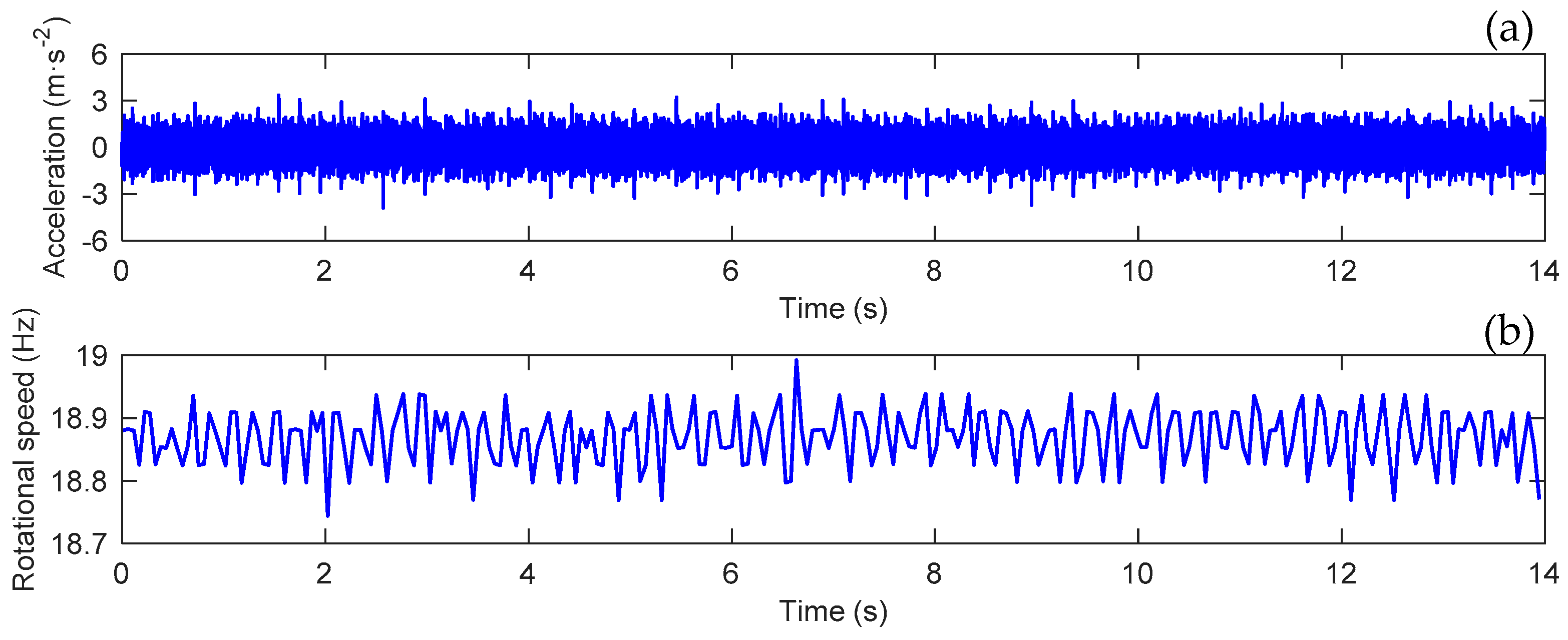
Figure 4a shows the vibration signal captured during the test of a faulty bearing. The test lasts for a duration of $L=14\mathrm{s}$. Figure 4b shows the rotational speed calculated from the tachometer signal using zero-cross detection method. It can be seen that the speed fluctuates between 18.9 Hz and 19.2 Hz around the mean value of $f_{\mathrm{r}}=19.06$ Hz. The mean speed of $f_{\mathrm{r}}$ can also be estimated from the amplitude spectrum of the vibration signals using higher order harmonics of the shaft frequency. With the estimated mean speed of $f_{\mathrm{r}}$, the fault frequency is calculated to be $f_{\mathrm{BF}}=75.93$ Hz and the fault period is $T_{\mathrm{BF}}=1/f_{\mathrm{BF}}=13.17\times {10}^{-3}$ s. The modulation frequency of the cage speed is $f_{\mathrm{c}}=7.27$ Hz. Thus, the cage revolves $\lfloor L·f_{\mathrm{c}}\rfloor =101$ whole cycles, allowing 101 LAIT segments to be separated for each roller.

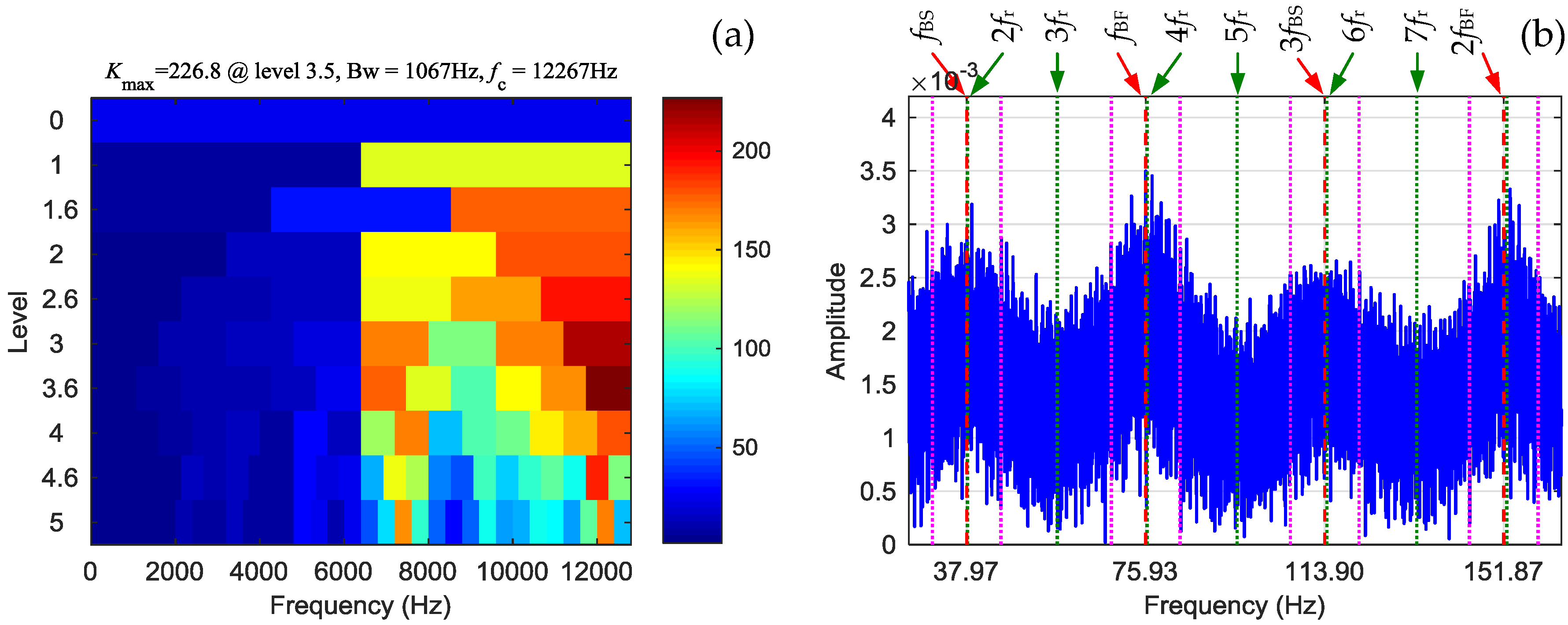
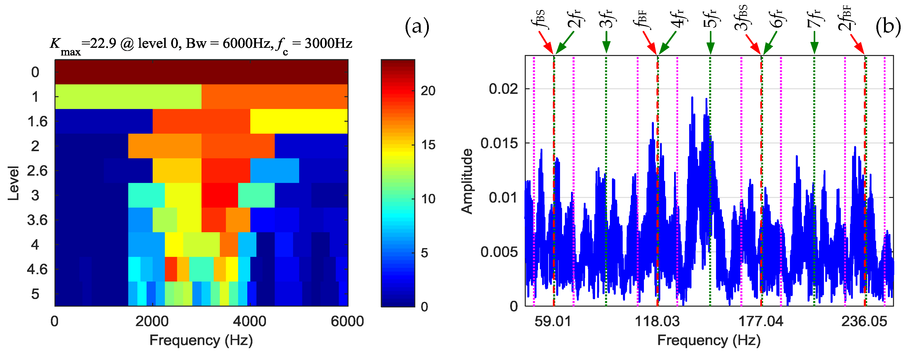
The Fast Kurtogram analysis result of the signal is shown in Figure 5a. An ‘optimal’ band of 11,733–12,800 Hz is selected. However, the signal in the band of the Fast Kurtogram can be affected by aliasing inevitably as the band is close to $f_{\mathrm{s}}/2$. Figure 5b shows the SES from the signal in the band of the Fast Kurtogram. It can be seen that the peaks at the spin frequency of $f_{\mathrm{BS}}$, the fault frequency of $f_{\mathrm{BF}}$ and their harmonics are badly smeared, owing to aliasing, speed oscillations and possible roller slippages. Smeared fault frequency component and high background noise cause high ambiguity in detecting the fault.

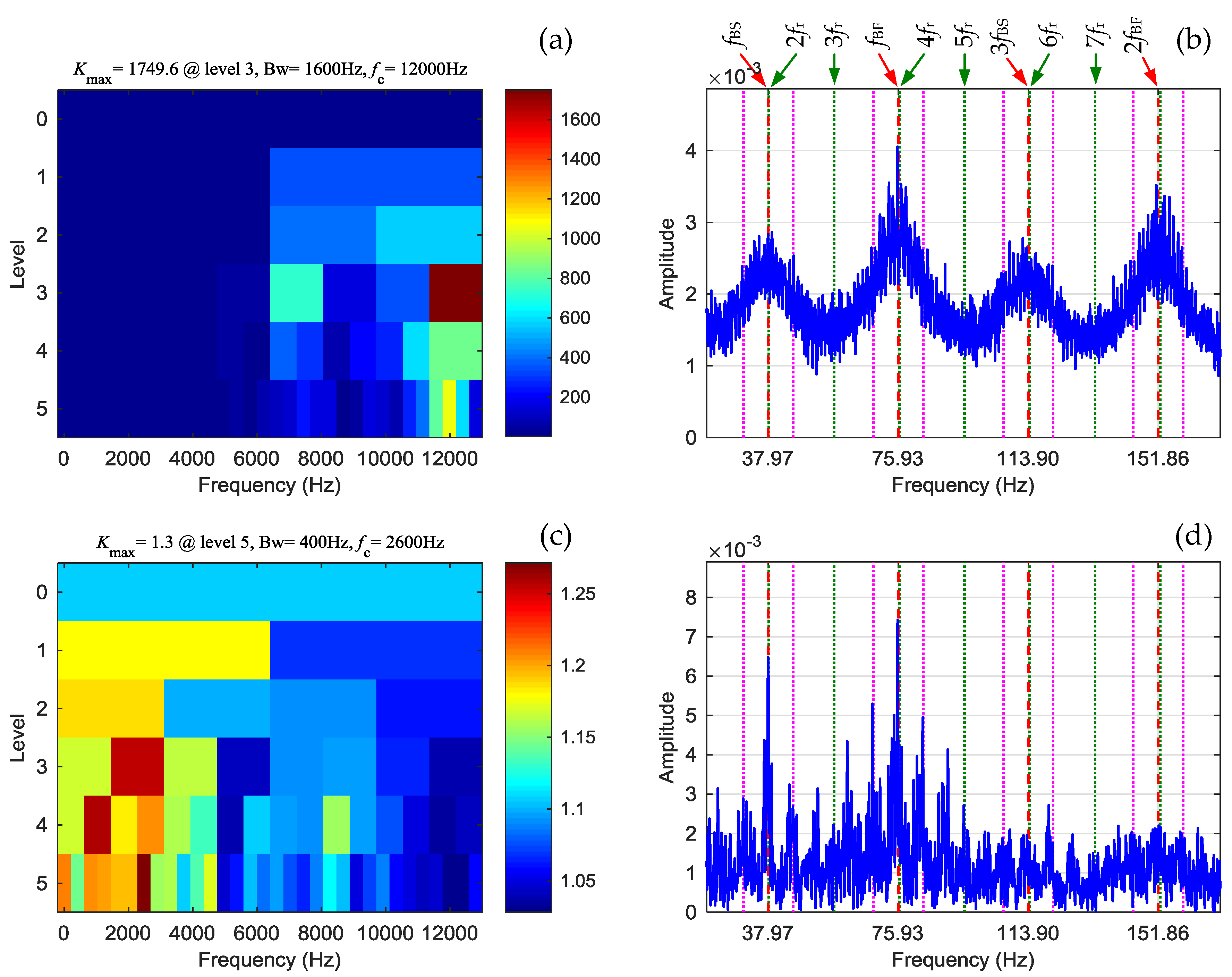
The Autogram selects a band of 11,200–12,800 Hz, which is also close to $f_{\mathrm{s}}/2$ as shown in Figure 6a. The SES from the Autogram is shown in Figure 6b which also shows badly smeared harmonics of the spin and fault frequencies. This may demonstrate that the Fast Kurtogram and Autogram can produce a biased band due to high nonstationarity and background noise. The Lower Autogram, which is more robust to large non-periodic impulses, selects a very distinct band of 2400–2800 Hz as shown in Figure 6c. The corresponding SES of the Lower Autogram is shown in Figure 6d, from which it can be seen that the peaks at the characteristic frequencies are much clearer. The SES of the Lower Autogram also reveals sidebands of the cage frequency around the spin and the fault frequencies. Although the characteristic frequency components and their sidebands are still smeared, they can be based on to indicate the existence of roller defects.

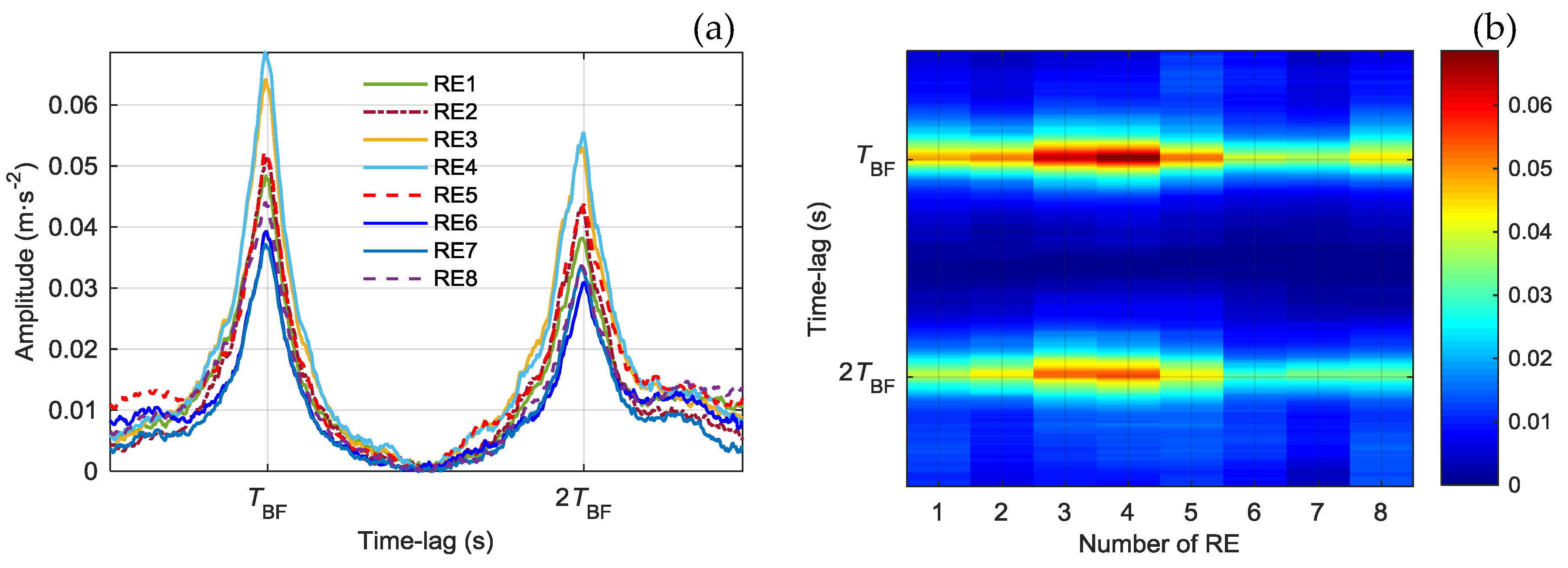
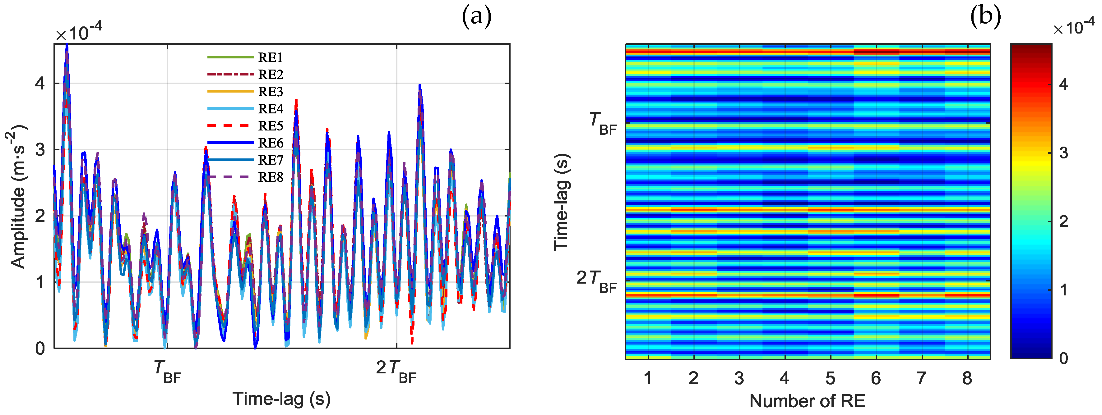
The LAIT-AEAs and their colour image yielded from the signals by performing the proposed method based on the LAIT separation and autocorrelation ensemble averaging are presented in Figure 7. It can be seen that the LAIT-AEAs of all rollers show two very clear peaks at the time-lags of $T_{\mathrm{BF}}$ and $2T_{\mathrm{BF}}$, indicating the existence of the frequency components at $f_{\mathrm{BF}}$ and $f_{\mathrm{BS}}$ respectively. From the colour image of the LAIT-AEAs, as shown in Figure 7b, it can be seen that the LAIT-AEAs have higher peak amplitudes in RE 3 and RE 4, and the peak amplitudes decrease from RE 4 to RE 6 in the clockwise direction and from RE 3 to RE 7 in the anticlockwise direction. The change features of the peak amplitudes indicate that bigger impulses are caused when RE 3 and RE 4 pass the load zone centre. These peaks as well as their change features illustrate that at least one of the rollers is defective and RE 3 or RE 4 is the most probably defective one.

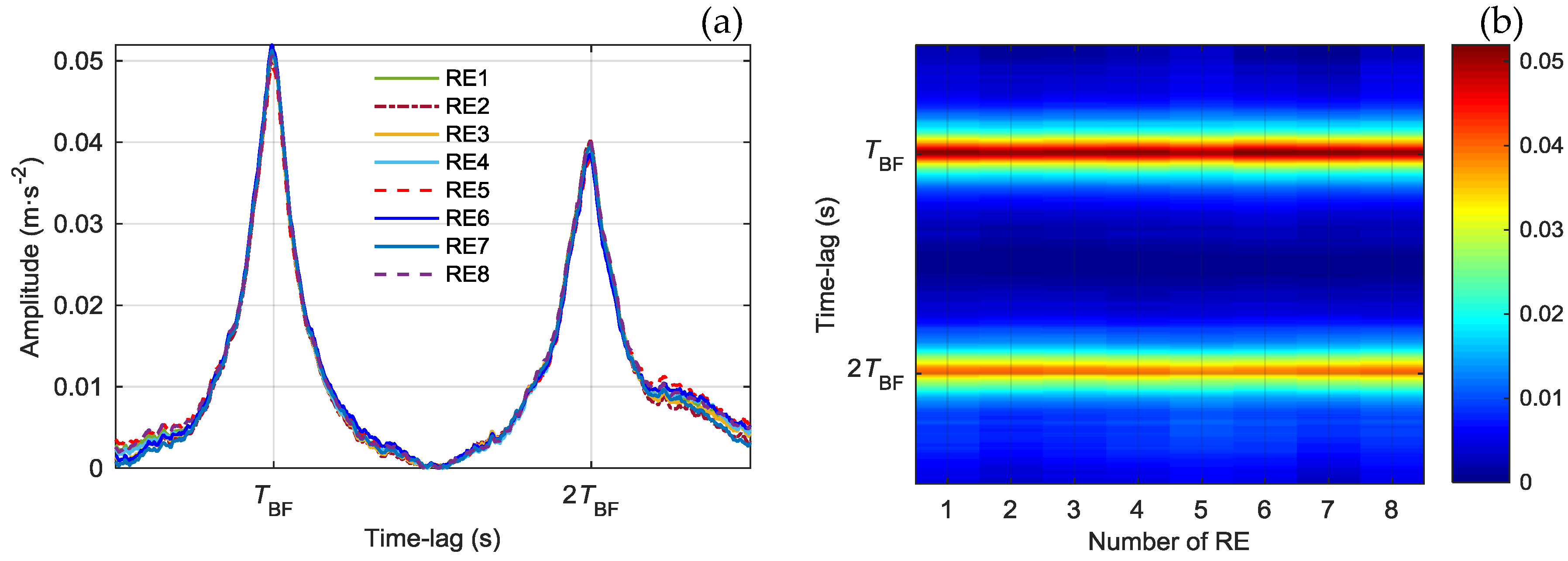
In the step of LAIT separation, the length of the LAIT segments is set using Equation (9), in which the subtended angle of the load zone is set to be $\mathsf{\pi }$. If the subtended angle of the load zone is set to $2\mathsf{\pi }$, the length of the separated segments spans a full cage rotation period, which means that the autocorrelation ensemble averaging in performed without LAIT separation. The corresponding AEAs and their colour image are shown in Figure 8, from which it can be seen that the AEAs of different rollers show peaks of almost equivalent amplitudes at the fault and the spin periods. The AEAs of a full cage rotation period do not give the information of the most probably defective roller any more. Moreover, the peak amplitudes of the AEAs are smaller than the amplitudes of the LAIT-AEAs of the most probably defective rollers. Thus, LAIT-AEAs can be more efficient than AEAs in case of high level background noise or other interfering components.

3.1.2. Healthy Case

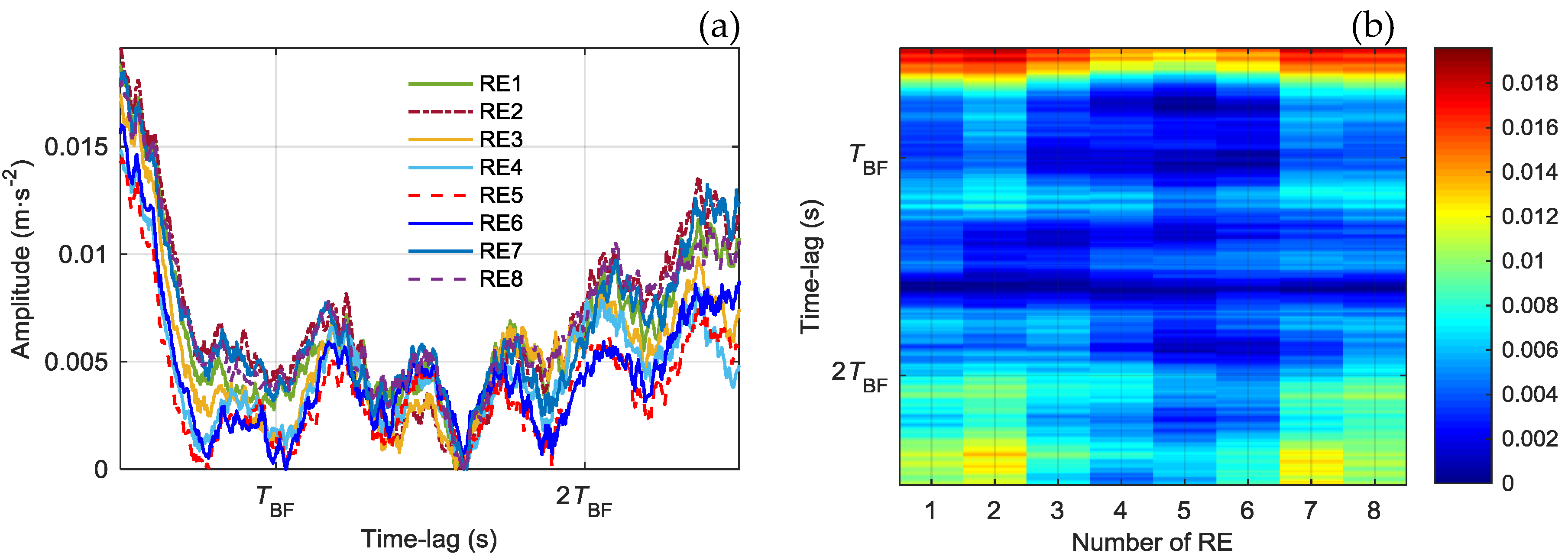
To verify that the LAIT-AEAs extracted from healthy bearings do not reveal the characteristic peaks at the time-lags of $T_{\mathrm{BF}}$ and $2T_{\mathrm{BF}}$, data collected from a healthy bearing is examined using the proposed method. Figure 9a,b show the vibration signal and rotational speed, respectively. The test also lasts for the duration of $L=14\mathrm{s}$. The speed fluctuates around the mean value of $f_{\mathrm{r}}=18.87$ Hz. The mean rotational speed can also be estimated from the vibration spectrum using higher order harmonics of the shaft frequency. The corresponding fault frequency is $f_{\mathrm{BF}}=75.18$ Hz and the fault period is $T_{\mathrm{BF}}=13.30\times {10}^{-3}$ s. The modulation frequency of the cage speed is $f_{\mathrm{c}}=7.20$ Hz. Thus, the cage revolves $\lfloor L·f_{\mathrm{c}}\rfloor =100$ whole cycles and 100 LAIT segments are separated for each roller. The LAIT-AEAs yielded for the healthy bearing signal are shown in Figure 10. It can be seen that the LAIT-AEAs extracted from the healthy bearing do not show the peaks at the time-lags of $T_{\mathrm{BF}}$ or $2T_{\mathrm{BF}}$, indicating that the bearing is in healthy condition. This then further verifies that the proposed method is reliable in indicating the fault of roller defects.

3.2. Validation with Case Western Reserve University Data

The dataset provided by the Case Western Reserve University Bearing Data Center [24] is publicly available and widely used to validate fault diagnostic methods of rolling element bearings. The details of the test bench which can be referred to the web of the Bearing Data Center will not be given here to save space. Here, three cases for defects on rollers and a case of baseline are examined by the proposed method.

3.2.1. Case 1: 291FE

The record of “291FE” from a fan end bearing is examined in this case. The bearing is a deep groove ball bearing with a defect of 0.53 mm at a roller. The roller fault frequency is $f_{\mathrm{BF}}=3.9874f_{\mathrm{r}}$ and the cage frequency is $f_{\mathrm{c}}=0.3817f_{\mathrm{r}}$. The sampling frequency is $f_{\mathrm{s}}=12$ kHz. According to the higher order harmonics of the shaft frequency, the estimated shaft frequency is $f_{\mathrm{r}}=29.6$ Hz. Thus, the fault frequency is $f_{\mathrm{BF}}=118.03$ Hz and the corresponding fault period is $T_{\mathrm{BF}}=8.47\times {10}^{-3}$ s. The cage frequency is $f_{\mathrm{c}}=11.30$ Hz. The duration of the signal is selected to be $L=10\mathrm{s}$, during which the cage revolves 113 whole cycles and 113 LAIT spins are separated for each roller.

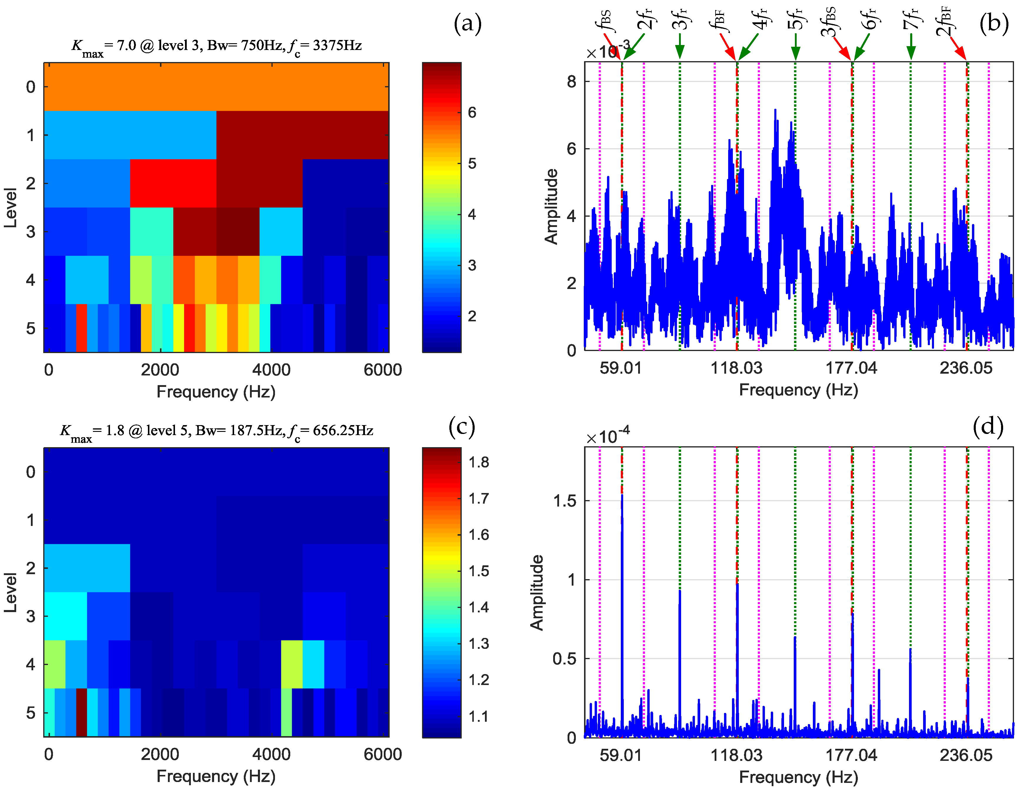
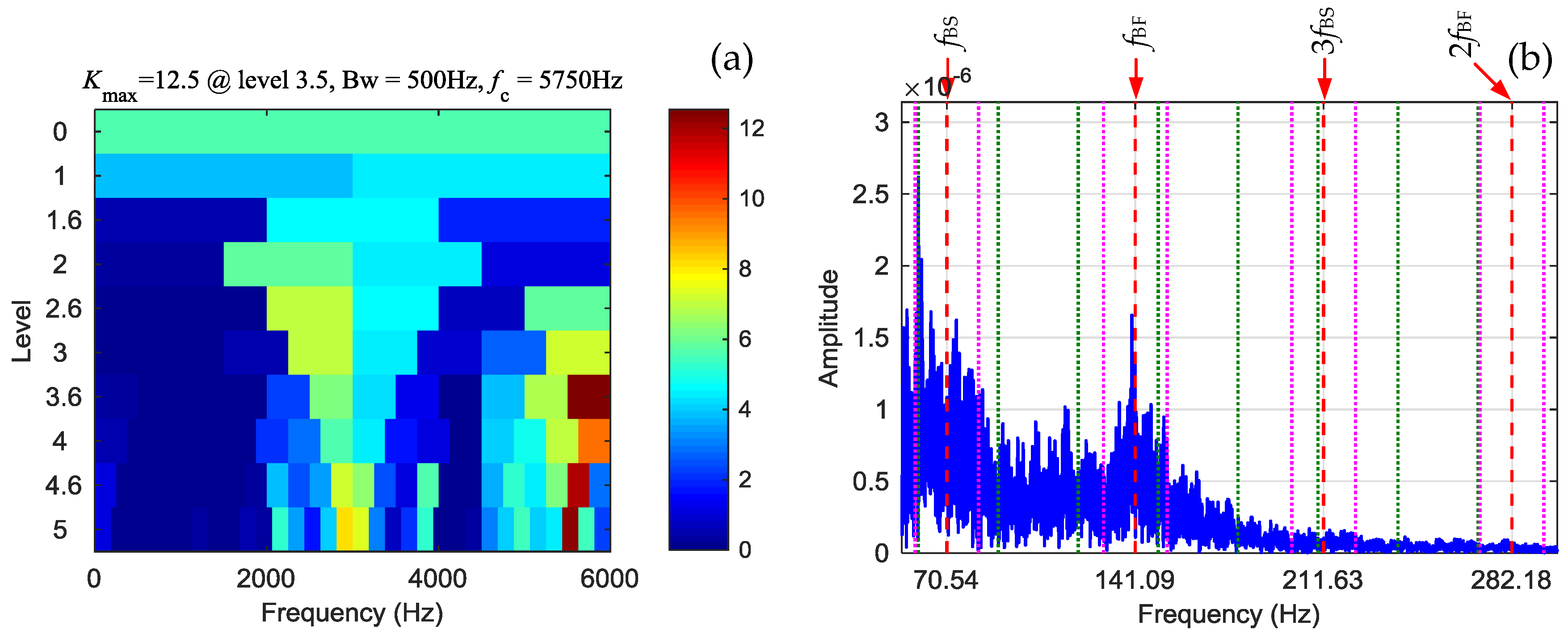
Figure 11 shows the Fast Kurtogram analysis result and the SES yielded from the Fast Kurtogram. It can be seen that the “optimal” band from the Fast Kurtogram is the whole band of 0–6000 Hz, which means that bandpass filtering does not have any effect at all. It can be seen from the SES that the component of the fault frequency and its harmonics are badly smeared and submerged in background noise and shaft components.

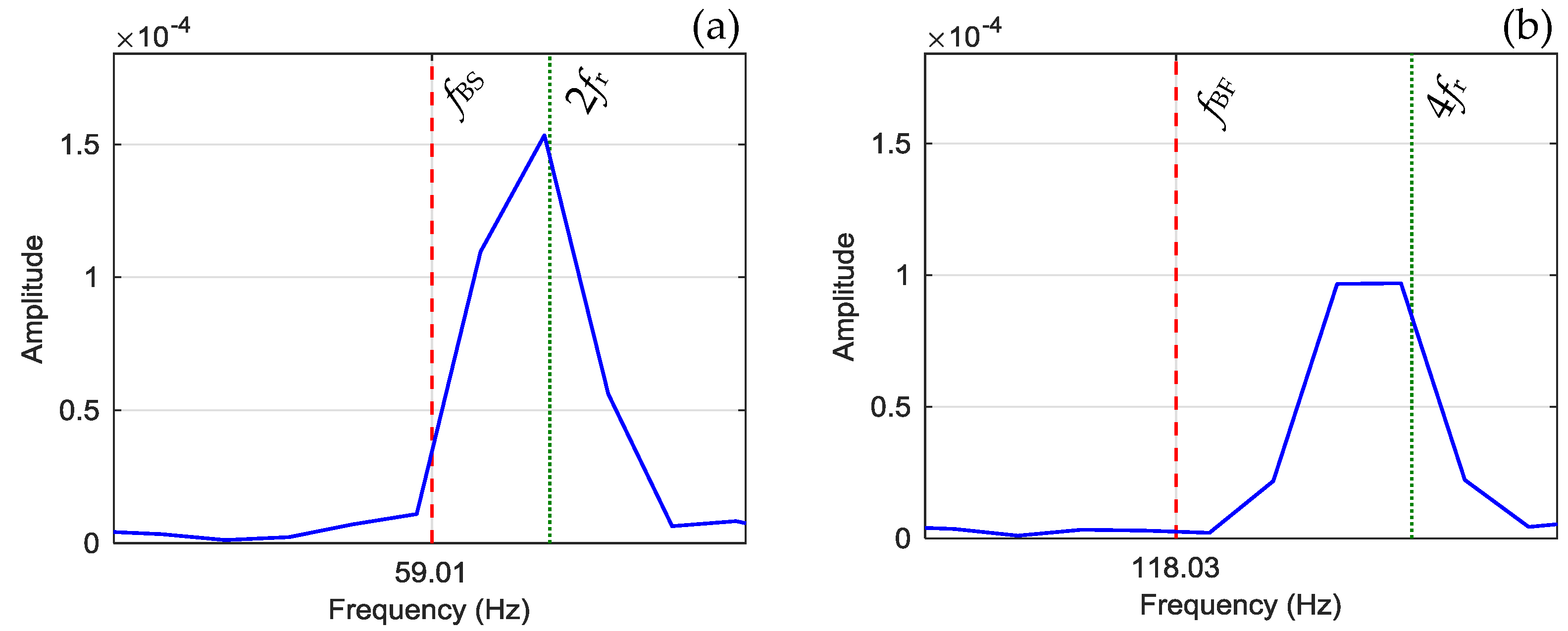
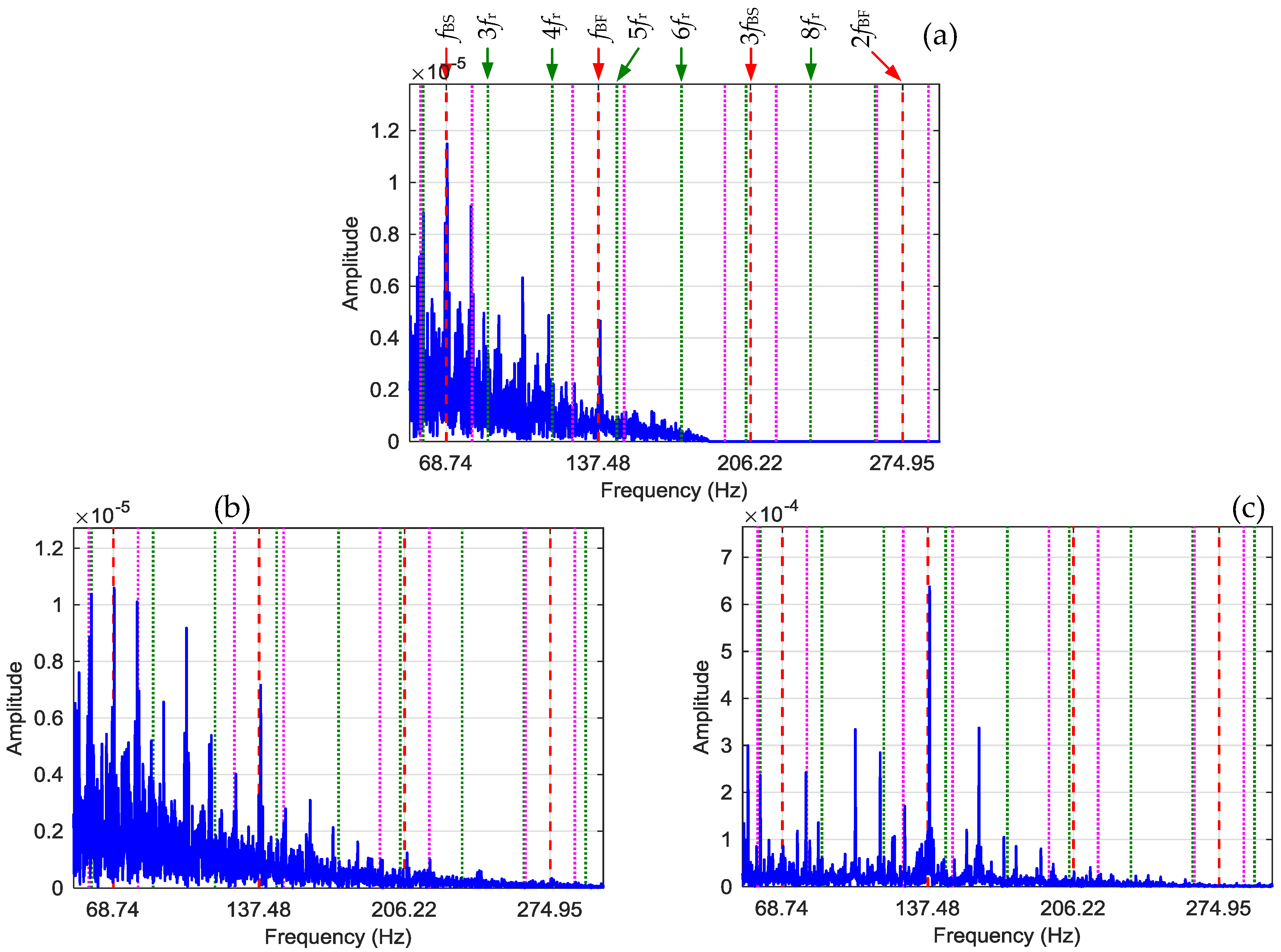
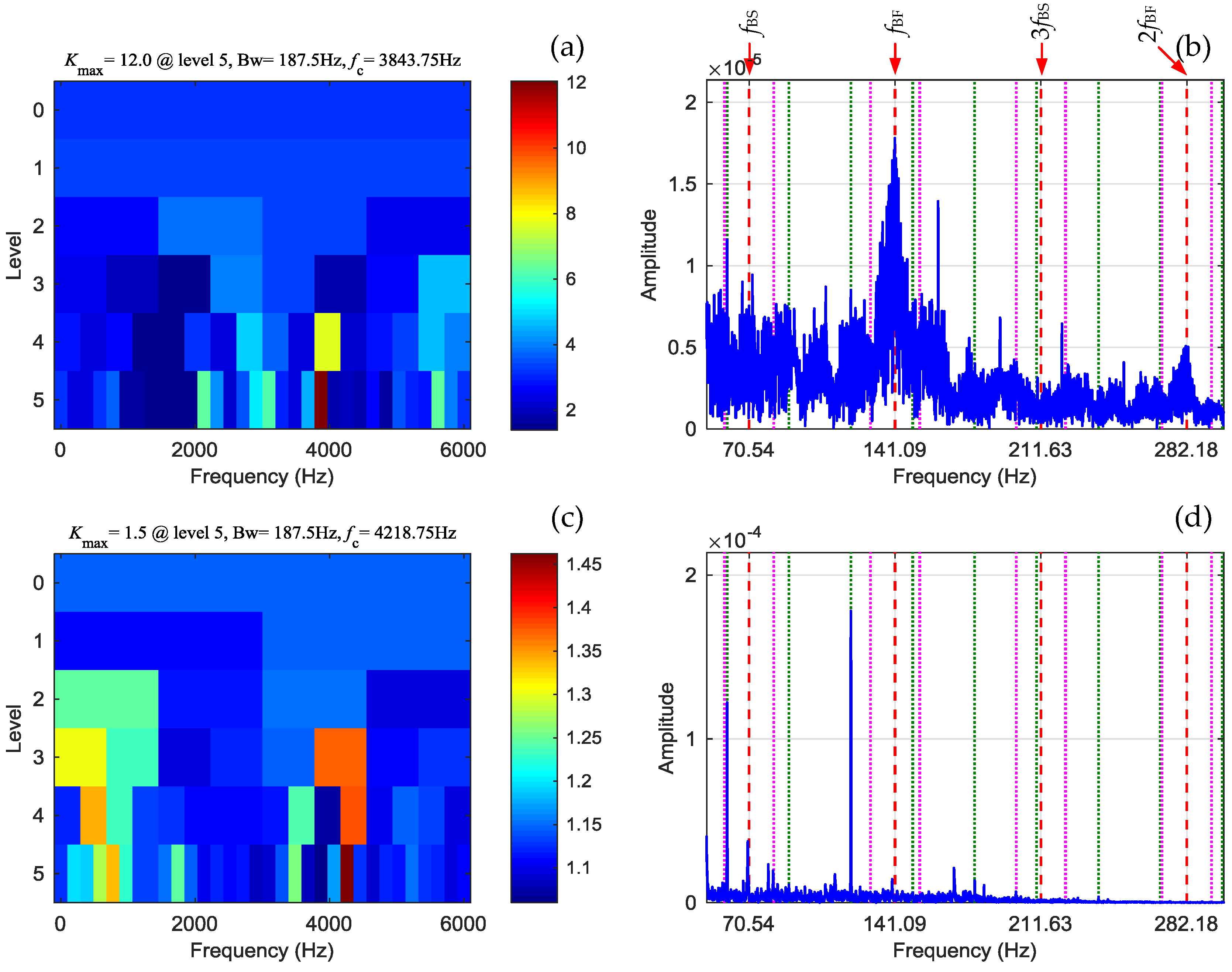
The band selected by the Autogram is 3000–3750 Hz as shown in Figure 12a. The SES yielded from the Autogram, as shown in Figure 12b, is also badly smeared and does not reveal the fault frequency harmonics either. The Lower Autogram selects a narrow band of 562.5–750 Hz as shown in Figure 12c, and the SES from this band is shown in Figure 12d. Although the “fault frequency harmonics” are clearly shown in the SES of the Lower Autogram, ambiguities in the diagnosis can be caused due to that the bearing fault frequencies are almost integer multiples of the shaft frequency. It is difficult to distinguish the roller fault frequency from the 4th order of the shaft frequency as they are so close to each other. This scenario happens for lots of bearings such as the bearings of MB ER-10K used in the machinery fault simulation bench as mentioned in Section 3.1. It must be noted that in the faulty case of the bearing of MB ER-10K, the odd-multiple order harmonics of the shaft frequency, which are far away from the fault frequency harmonics, cannot be seen from the SES of the Lower Autogram as shown in Figure 6. In the case of 291FE, the odd-multiple order harmonics of the shaft frequency are also shown in the SES along with the fault frequency harmonics or the even-multiple order harmonics of the shaft frequency. Moreover, from the partial enlarged detail of the SES as shown in Figure 13, it can be seen that the interesting components are closer to the 2nd and 4th order harmonics of the shaft frequency rather than to the roller spin and fault frequencies.

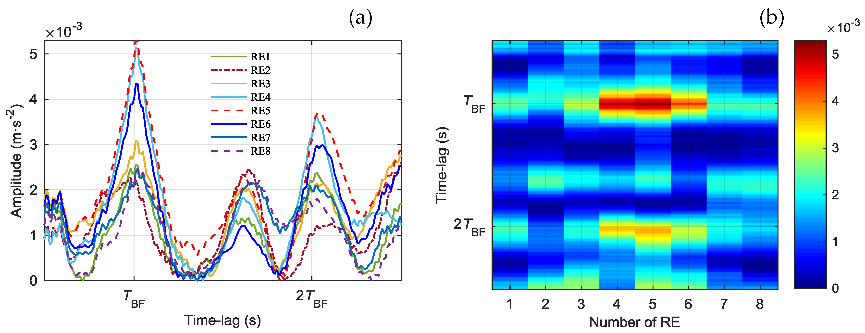
Figure 14 shows the LAIT-AEAs and their colour image yielded in this case. It can be seen that the LAIT-AEAs show clear peaks at the time-lags of $T_{\mathrm{BF}}$ and $2T_{\mathrm{BF}}$. Certainly, these two period components can also be deemed as the 4th and 8th order harmonics of the shaft frequency. However, a conclusion of roller defect can be drawn according to the colour image of the LAIT-AEAs as shown in Figure 14b. Particularly, the LAIT-AEA of RE 5 has the highest peak amplitudes, and the peak amplitudes decrease generally from RE 5 to the rollers further away in both clockwise and anticlockwise directions. These peaks together with their change features indicate that at least one of the rollers is defective and RE 5 is the most probably defective one.

3.2.2. Case 2: 3007DE

In this case, the record of “3007DE” from a drive end bearing is examined. A defect of 0.71 mm was introduced at a roller of the bearing. The roller fault frequency is $f_{\mathrm{BF}}=4.7135f_{\mathrm{r}}$ and the cage frequency is $f_{\mathrm{c}}=0.39828f_{\mathrm{r}}$. The sampling frequency is $f_{\mathrm{s}}=12$ kHz. The shaft frequency estimated according to the higher order harmonics of the shaft frequency is 29.2 Hz. Thus, the fault frequency is 137.48 Hz and the corresponding fault period is $7.27\times {10}^{-3}$ s. The cage frequency is 11.62 Hz. The cage revolves 116 whole cycles in the time interval of 10 s, and 116 LAIT segments are separated for each roller.

Three different bands are selected by the Fast Kurtogram, Autogram and Lower Autogram. The SESs yielded from these three bands are shown in Figure 15. All the SESs reveal the roller characteristic frequencies and the sidebands of the cage frequency, indicating the existence of roller defect.

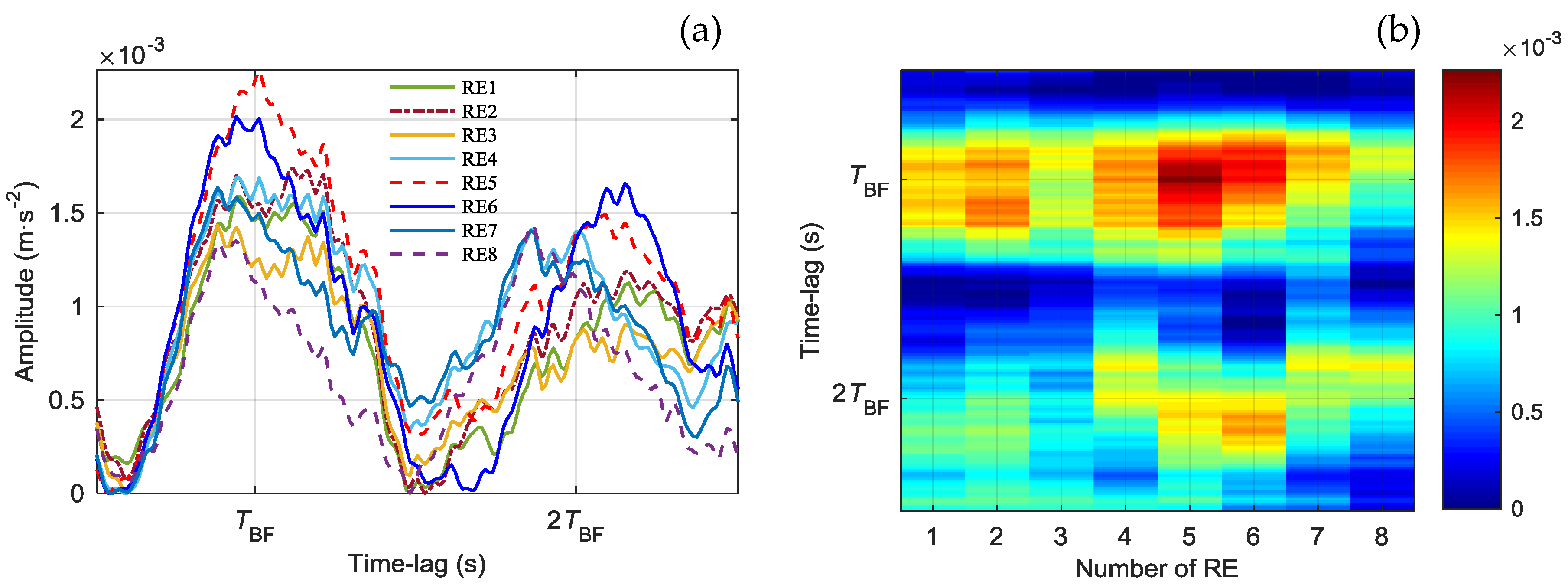
The LAIT-AEAs and their colour image yielded from this case are shown in Figure 16. It can be seen that the LAIT-AEAs show clear peaks at the time-lags of $T_{\mathrm{BF}}$ and $2T_{\mathrm{BF}}$, corresponding to the fault frequency and the spin frequency respectively. In addition, the LAIT-AEAs also clearly exhibit the 4th order harmonic of the fault frequency. This is probably because there is more the one defect on the roller or more than one roller is defective. The change feature that the peak amplitudes decrease gradually from a roller to the rollers that are further away are not clear enough owing to the same reason.

3.2.3. Case 3: 222DE

The record of “222DE” was captured from a drive end bearing with a roller defect of 0.53 mm. The shaft frequency estimated from the amplitude spectrum of the vibration using higher order harmonics of the shaft frequency is 29.93 Hz. The corresponding fault frequency is 141.09 Hz and the fault period is $7.09\times {10}^{-3}$ s. The cage speed is 11.92 Hz; thus, the cage revolves 119 whole cycles in 10 s and 119 LAIT segments are separated for each roller.

Figure 17a shows the analysis result of the Fast Kurtogram. A band of 5500–6000 Hz is selected and the band is close to $f_{\mathrm{s}}/2$. Figure 17b shows the SES yielded from this band, from which it can be seen that only the 1st order harmonic of the fault frequency is revealed, but the component still shows high smearing effects. The component of the spin frequency as well as the high order harmonics of the characteristic frequencies is submerged.

Figure 18a,c show two different bands selected by the Autogram and the Lower Autogram. The SES of the Autogram, as shown in Figure 18b, exhibits the 1st and 2nd order harmonics of the fault frequency. And these two components are badly smeared. The 1st and 3rd order harmonics of the spin frequency cannot be seen. As for the SES of the Lower Autogram as shown in Figure 18d, the components of the characteristic frequencies are submerged in the components of the shaft frequency.

Figure 19 shows the LAIT-AEAs and their color image calculated from the signal. It can be seen that the LAIT-AEAs show clear peaks near the time-lags of $T_{\mathrm{BF}}$ and $2T_{\mathrm{BF}}$, indicating the existence of the components of $f_{\mathrm{BF}}$ and $f_{\mathrm{BS}}$. Although the peaks are skewed probably by the influences of speed fluctuations, roller slippages and so on, the peaks of $T_{\mathrm{BF}}$ and $2T_{\mathrm{BF}}$ can be based on to indicate the existence of roller defects. In addition, the LAIT-AEAs have higher peak amplitudes in RE 5 and RE 6, indicating that bigger impulses are caused when these two rollers pass the load zone centre and one of them is most probably defective.

3.2.4. Case 4: Baseline of 100DE

Healthy bearing cases are also examined as baselines using the proposed method. Figure 20 shows LAIT-AEAs and their colour image yielded from the record of “100DE”. The shaft frequency is 28.83 Hz. The corresponding roller fault frequency is $f_{\mathrm{BF}}=135.91$ Hz and the fault period is $7.36\times {10}^{-3}$ s. The cage frequency is $f_{\mathrm{c}}=11.48$ Hz. The cage revolves 114 whole cycles in 10 s and 114 LAIT segments are separated for each roller. It can be seen from Figure 20 that the LAIT-AEAs do not show the peaks at $T_{\mathrm{BF}}$ or $2T_{\mathrm{BF}}$, indicating that the bearing has no roller defects. This then further verifies that the proposed method is reliable.

4. Conclusions

A fault diagnostic method based on AEA of LAIT segments is proposed for rolling element bearings. According to the bearing kinematics and the characteristic that a defective roller causes LAITs when passing the load zone centre, this method separates the LAIT segments for achieving higher SNR signals. After demodulation, the separated LAIT segments are further aligned with autocorrelation and enhanced with ensemble averaging. In this way, a signature named LAIT-AEA is yielded for each roller. The LAIT-AEAs with peaks at the time-lags of $T_{\mathrm{BF}}$ and $2T_{\mathrm{BF}}$ can be referred to as reliable indicators of roller defects. This method is evaluated with different datasets, showing that it can be very effective and convenient for real-time and online applications because of its key merits: (1) bandpass filtering is not involved and thus the method does not rely on band selection; (2) the method is sensitive to roller defect and gives the information of the most probably defective roller; (3) the method is robust to speed fluctuations and roller slippages since the LAIT segments are demodulated and aligned with autocorrelation; (4) the method has low computation load, as only time-domain signal processing techniques are used and the techniques are applied to short LAIT segments.

References

- Malla, C.; Panigrahi, I. Review of condition monitoring of rolling element bearing using vibration analysis and other techniques. J. Vib. Eng. Technol. 2019, 7, 407–414. [Google Scholar] [CrossRef]
- Tandon, N.; Choudhury, A. An analytical model for the prediction of the vibration response of rolling element bearings due to a localized defect. J. Sound Vib. 1997, 205, 275–292. [Google Scholar] [CrossRef]
- Randall, R. Vibration-Based Condition Monitoring: Industrial, Aerospace and Automotive Applications; John Wiley & Sons Ltd Publication: Hoboken, NJ, USA, 2011. [Google Scholar]
- Darlow, M.; Badgley, R.; Hogg, G. Application of high-frequency resonance techniques for bearing diagnostics in helicopter gearboxes. In Tech Rep; Mechanical Technology Inc.: Latham, NY, USA, 1974. [Google Scholar]
- McFadden, P.; Smith, J. Vibration monitoring of rolling element bearings by the high frequency resonance technique–a review. Tribol. Int. 1974, 17, 3–10. [Google Scholar] [CrossRef]
- Randall, R. Modern envelope analysis for bearing diagnostics. In Proceedings of the 28th International Congress of Condition Monitoring and Diagnostic Engineering Management and the 10th Regional Non-Destructive & Structural Testing Congress, Buenos Aires, Argentina, 14 December 2015. [Google Scholar]
- Antoni, J. Fast computation of the Kurtogram for the detection of transient faults. Mech. Syst. Signal Process. 2007, 21, 108–124. [Google Scholar] [CrossRef]
- Barszcz, T.; Jablonski, A. A novel method for the optimal band selection for vibration signal demodulation and comparison with the kurtogram. Mech. Syst. Signal Process. 2011, 25, 431–451. [Google Scholar] [CrossRef]
- Moshrefzadeh, A.; Fasana, A. The Autogram: An effective approach for selecting the optimal demodulation band in rolling element bearings diagnosis. Mech. Syst. Signal Process. 2017, 105, 294–318. [Google Scholar] [CrossRef]
- Tian, X.; Gu, J.; Rehab, I.; Abdalla, G.; Gu, F.; Ball, A. A robust detector for rolling element bearing condition monitoring based on the modulation signal bispectrum and its performance evaluation against the Kurtogram. Mech. Syst. Signal Process. 2018, 100, 167–187. [Google Scholar] [CrossRef]
- Braun, S. The extraction of periodic waveforms by time domain averaging. Acta Acust. United Acust. 1975, 32, 69–77. [Google Scholar]
- Braun, S. The synchronous (time domain) average revisited. Mech. Syst. Signal Process. 2011, 25, 1087–1102. [Google Scholar] [CrossRef]
- Halim, E.B.; Choudhury, M.A.A.; Shah, S.L.; Zou, M.J. Time domain averaging across all scales: A novel method for detection of gearbox faults. Mech. Syst. Signal Process. 2008, 22, 261–278. [Google Scholar] [CrossRef]
- Zhao, M.; Lin, J.; Lei, Y.; Wang, X. Flexible Time Domain Averaging Technique. Chin. J. Mech. Eng. 2013, 26, 1022–1030. [Google Scholar] [CrossRef]
- Stewart, R.M. Some Useful Data Analysis Techniques for Gearbox Diagnostics; Report MHM/R/10/77; Machine Health Monitoring Group, Institute of Sound and Vibration Research, University of Southampton: Southampton, UK, July 1977. [Google Scholar]
- McFadden, P. A technique for calculating the time domain averages of the vibration of the individual planet gears and the sun gear in an epicyclic gearbox. J. Sound Vib. 1991, 144, 163–172. [Google Scholar] [CrossRef]
- Siegel, D.; Al-Atat, H.; Shauche, V.; Liao, L.; Snyder, J.; Lee, J. Novel method for rolling element bearing health assessment—A tachometer-less synchronously averaged envelope feature extraction technique. Mech. Syst. Signal Process. 2012, 29, 362–376. [Google Scholar] [CrossRef]
- McFadden, P.; Toozhy, M. Application of synchronous averaging to vibration monitoring of rolling element bearing. Mech. Syst. Signals Process. 2000, 14, 891–906. [Google Scholar] [CrossRef]
- McFadden, P.; Smith, J. Model for the vibration produced by a single point defect in a rolling element bearing. J. Sound Vib. 1984, 96, 69–82. [Google Scholar] [CrossRef]
- Randall, R.; Antoni, J. Rolling element bearing diagnostics–A tutorial. Mech. Syst. Signal Process. 2011, 25, 485–520. [Google Scholar] [CrossRef]
- Hu, L.; Zhang, L.; Gu, F.; Hu, N.; Ball, A. Extraction of the largest amplitude impact transients for diagnosing rolling element defects in bearings. Mech. Syst. Signal Process. 2019, 116, 796–815. [Google Scholar] [CrossRef] [Green Version]
- Singh, J.; Darpe, A.; Singh, S. Rolling element bearing fault diagnosis based on over-complete rational dilation wavelet transform and auto-correlation of analytic energy operator. Mech. Syst. Signal Process. 2018, 100, 662–693. [Google Scholar] [CrossRef]
- Smith, W.; Randall, R. Rolling element bearing diagnostics using the Case Western Reserve University data: A benchmark study. Mech. Syst. Signal Process. 2015, 64, 100–131. [Google Scholar] [CrossRef]
- Case Western Reserve University Bearing Data Center Website. Available online: http://csegroups.case.edu/bearingdatacenter/home (accessed on 20 June 2019).
Figure 1.
Averaging results of signal segments with different cases of transients: (a) case for neither modulation nor phase error; (b) case for modulation but no phase error; (c) case for both modulation and phase errors.
Figure 2.
Flowchart of the diagnostic method based on AEA of LAIT segments.
Figure 3.
Machinery fault simulation bench.
Figure 4.
Faulty case: (a) raw vibration signals; (b) rotational speed.
Figure 5.
Faulty case: (a) Fast Kurtogram result; (b) SES from Fast Kurtogram.
Figure 6.
Faulty case: (a) Autogram result; (b) SES from Autogram; (c) Lower Autogram result; (d) SES from Lower Autogram.
Figure 7.
Faulty case: (a) LAIT-AEAs; (b) colour image of LAIT-AEAs.
Figure 8.
Faulty bearing: (a) AEAs yield from segments of a full cage rotation period; (b) colour image of AEAs.
Figure 9.
Healthy case: (a) raw vibration signals; (b) rotational speed.
Figure 10.
Healthy case: (a) LAIT-AEAs; (b) colour image of LAIT-AEAs.
Figure 11.
Case 1 of 291FE: (a) Fast Kurtogram result; (b) SES from Fast Kurtogram.
Figure 12.
Case 1 of 291FE: (a) Autogram result; (b) SES from Autogram; (c) Lower Autogram result; (d) SES from Lower Autogram.
Figure 13.
Case 1 of 291FE: (a) partial enlarged detail of SES around spin frequency; (b) partial enlarged detail of SES around faulty frequency.
Figure 14.
Case 1 of 291FE: (a) LAIT-AEAs; (b) colour image of LAIT-AEAs.
Figure 15.
Case 2 of 3007DE: (a) SES from Fast Kurtogram; (b) SES from Autogram; (c) SES from Lower Autogram.
Figure 16.
Case 2 of 3007DE: (a) LAIT-AEAs; (b) colour image of LAIT-AEAs.
Figure 17.
Case 3 of 222DE: (a) Fast Kurtogram result; (b) SES from Fast Kurtogram.
Figure 18.
Case 3 of 222DE: (a) Autogram result; (b) SES from Autogram; (c) Lower Autogram result; (d) SES from Lower Autogram.
Figure 19.
Case 3 of 222DE: (a) LAIT-AEAs; (b) colour image of LAIT-AEAs.
Figure 20.
LAIT-AEAs of data “100DE” yielded with Band 2: (a) LAIT-AEAs and (b) colour image of LAIT-AEAs.
© 2019 by the authors. Licensee MDPI, Basel, Switzerland. This article is an open access article distributed under the terms and conditions of the Creative Commons Attribution (CC BY) license (http://creativecommons.org/licenses/by/4.0/).
Share and Cite
MDPI and ACS Style
Hu, L.; Xu, Y.; Gu, F.; He, J.; Hu, N.; Ball, A. Autocorrelation Ensemble Average of Larger Amplitude Impact Transients for the Fault Diagnosis of Rolling Element Bearings. Energies 2019, 12, 4740. https://doi.org/10.3390/en12244740
AMA Style
Hu L, Xu Y, Gu F, He J, Hu N, Ball A. Autocorrelation Ensemble Average of Larger Amplitude Impact Transients for the Fault Diagnosis of Rolling Element Bearings. Energies. 2019; 12(24):4740. https://doi.org/10.3390/en12244740
Chicago/Turabian StyleHu, Lei, Yuandong Xu, Fengshou Gu, Jing He, Niaoqing Hu, and Andrew Ball. 2019. "Autocorrelation Ensemble Average of Larger Amplitude Impact Transients for the Fault Diagnosis of Rolling Element Bearings" Energies 12, no. 24: 4740. https://doi.org/10.3390/en12244740
Note that from the first issue of 2016, this journal uses article numbers instead of page numbers. See further details here.