Cost Uncertainties in Energy System Optimization Models: A Quadratic Programming Approach for Avoiding Penny Switching Effects


1
Institute of Electrochemical Process Engineering (IEK-3), Forschungszentrum Jülich GmbH, Wilhelm-Johnen-Str., 52428 Jülich, Germany
2
Chair of fuel cells, RWTH Aachen University, c/o Institute of Electrochemical Process Engineering (IEK-3), Forschungszentrum Jülich GmbH, Wilhelm-Johnen-Str., 52428 Jülich, Germany
*
Author to whom correspondence should be addressed.
Energies 2019, 12(20), 4006; https://doi.org/10.3390/en12204006
Submission received: 25 July 2019
/
Revised: 9 October 2019
/
Accepted: 20 October 2019
/
Published: 21 October 2019
(This article belongs to the Special Issue Model Coupling and Energy Systems)
Abstract
:Designing the future energy supply in accordance with ambitious climate change mitigation goals is a challenging issue. Common tools for planning and calculating future investments in renewable and sustainable technologies are often linear energy system models based on cost optimization. However, input data and the underlying assumptions of future developments are subject to uncertainties that negatively affect the robustness of results. This paper introduces a quadratic programming approach to modifying linear, bottom-up energy system optimization models to take cost uncertainties into account. This is accomplished by implementing specific investment costs as a function of the installed capacity of each technology. In contrast to established approaches such as stochastic programming or Monte Carlo simulation, the computation time of the quadratic programming approach is only slightly higher than that of linear programming. The model’s outcomes were found to show a wider range as well as a more robust allocation of the considered technologies than the linear model equivalent.
1. Introduction
There are various concepts and ideas relating to how to design the future energy supply to achieve the climate goals set out in the Paris Agreement of 2015. These design concepts normally rely on energy scenarios that are influenced by various uncertainties. As a consequence, it is very challenging for decision-makers to devise robust solutions to reach the aforementioned goals. Thus, the underlying decision-making process is supported by different types of energy system models. Most of these focus on the identification of cost-efficient options to supply future energy demand [1]. Due to their complexity, the models are often limited to linear programming (LP) or mixed-integer linear programming (MILP) [2,3]. However, the input data and boundary conditions for modeling future energy systems are invariably subject to uncertainties, regardless of whether simulation or optimization models are considered [4,5,6]. In particular, social, climatological, and technological developments constitute momentous and influential factors on the model’s results [7,8]. For the consideration of social factors, the incorporation of consumer behavior in energy system models represents an essential aspect. An approach to this is presented, for instance, in the TIMES (The Integrated MARKAL-EFOM System) model, which aims at extending the model details by integrating the heterogeneity of consumers [9,10]. On the other side, an example of uncertainties in the assumptions on technological developments is the future investment costs of technologies [11,12] Minimal changes to these assumptions on developments may induce marked differences in the resulting shares of technologies in the energy system. Linear cost optimization models, in particular, are affected by this so-called ‘penny switching effect’, which leads to a complete switch to other technologies through marginal variations in the corresponding investment costs [13,14,15]. This results in the underestimation of certain technologies or even of entire supply chains. For this reason, linear optimization models are highly sensitive to input parameters, such as investment costs. Moreover, many technologies are not considered in the results of such models due to having marginally higher costs than a comparable alternative technology.
Existing solutions to overcome the described issues include, for instance, stochastic programming, Monte Carlo simulation, and sensitivity analyses [11,16,17,18]. All of these approaches have one thing in common. Namely, they are based on a parameter variation that is accompanied by substantial computational efforts. To obtain more robust results with acceptable computational efforts, this paper describes an approach that aims to take investment cost uncertainties into account, with only a slight increase in the required computation time. For that purpose, a linear bottom-up energy system model for Germany is modified. Instead of a default value for specific investment costs, a cost range is implemented as a function of the installed capacity of each technology. This results in a convex quadratic objective function of the model intended to minimize the total system costs. As a consequence, the model’s results are expected to comprise a wider range of technologies, be more robust, and, thus, more realistic.
2. Methods
All of the results presented in this paper show potential for the strategy to reduce German CO2 emissions by 80% against the reference year of 1990, taking into account both energy-related and process-related emissions. The underlying model comprises the energy sector, as well as the end-use sectors: buildings, transport, and industry. Other sectors, such as the agricultural sector and greenhouse gases other than CO2, were not included. The year 2050 was chosen as the target year in this paper to provide an indication of the necessary transformation of the German energy system to implement the Federal Government’s greenhouse gas reduction targets.
For that reason, the cross-sectoral, myopic energy system model ‘FINE-NESTOR’ (National Energy System model with integrated SecTOR coupling, https://github.com/FZJ-IEK3-VSA/FINE) was used to determine the results and the corresponding CO2 reduction strategy. A detailed description of the model framework can be found in Welder et al. (2018) [19]. The analysis of the energy system’s transformation was subject to an interval of five years, starting from today’s energy system and progressing up to the year 2050. Depending on the setup, this can be run in LP or quadratic programming (QP) mode based on the implementation of investment costs. The model did not consider spatial aspects of energy supply and demand but had a flexible temporal resolution. The latter was set to an hourly basis, and so amounted to 8760 time steps. Additionally, the temporal resolution could be reduced by the aggregation of typical days. The corresponding approach is described by Kotzur et al. (2017, 2018) [20,21]. In this context, the intra-year use of storage technologies relied on a perfect-foresight approach. Finally, each year was individually optimized with the objective of minimizing the total annual system costs.
The underlying framework conditions of the optimization of each year were based on historical data and the results of previously calculated years. At this point, the decommissioning of existing plants and a maximum annual expansion rate for each technology was taken into account. These expansion rates were based on learning curves, employment effects, and technical potentials. In combination with minimum annual expansion targets based on fundamental market diffusion curves and the optimized installed capacities of the target year, the upper and lower bounds for the optimization were determined. However, the depicted results only relate to the target year. The preceding myopic transformation of the energy system was not considered in this analysis, except for comparison purposes. Moreover, the presented results aim to support the hypotheses of this paper as well as to reveal the effects of the described methodology. They do not represent forecasts or recommendations for the future development of the energy system of Germany.
The most important underlying input data of the model is summarized in the following. Assumptions on demographic and macroeconomic developments, as well as fuel price tendencies, were primarily adopted from Buerger et al. (2016) and Gerbert et al. (2018) [22,23]. Electricity and heat demand profiles, as well as the supply profiles of PV and wind power plants, were based on historical data from the year 2013. Decisive techno–economic input parameters are shown in the Appendix A, Table A1. This provided an abstract of around 900 components and 1500 energy and mass flows implemented in the model.
3. Investment Cost Analysis
With regard to the future energy supply being in compliance with the climate goals of the Paris Agreement, renewable energy technologies will play a key role. In contrast to fossil power generation, the output of these technologies is not bound to fuel costs. Instead, capital expenditures (CAPEX) are the crucial factor when it comes to investment decisions. This leads to planning tools, such as energy system models, being very sensitive towards the assumed CAPEX, which in turn are mainly affected by the initial investment.
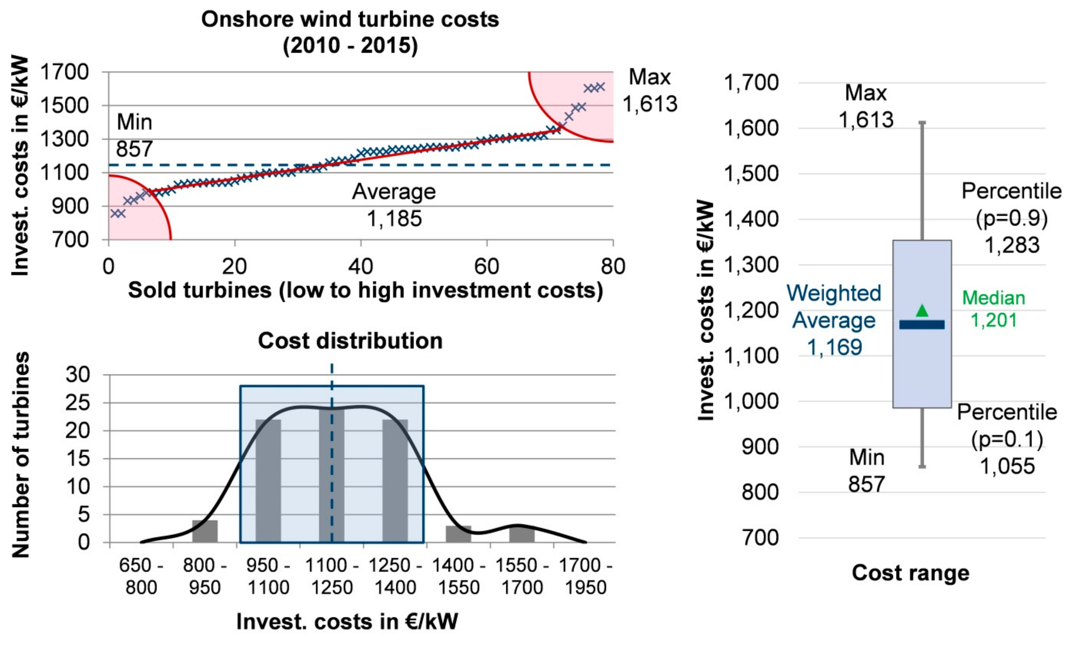
When looking into the historical investment costs of renewable energy technologies, it is notable that the specific costs per kilowatt vary significantly. On the one hand, economies of scale, as well as the resulting increase in manufacturing efficiency, have been the major influencing factors on renewable energy costs over the last decades. Other important factors that impact the actual costs of an individual technology or project relate to market pricing, auction designs, technological developments, and geographical aspects, such as ground conditions or local construction and transport costs [24,25,26]. The approach described in this paper focuses on the latter aspects. Because these kinds of influencing factors are very dependent on the exact location and the individual construction project, they are hard to predict beforehand in higher-level planning processes. Therefore, these influencing factors are considered as uncertainties in the context of this paper. The impact of all of these influencing factors on the investment costs of renewable energies will be shown by the example of onshore wind turbines in the following. To exclude the effect of learning curves and economies of scale as precisely as possible, a short and current period of realized investments in onshore wind turbines is the object of investigation. The resulting deviations in investment costs are depicted in Figure 1. This graphic illustrates the investment cost range and deviation of 80 wind turbines that were constructed between 2010 and 2015. Their specific investment costs per kilowatt in ascending order from low to high costs are shown in the upper left-hand corner. The minimum costs were 857 €/kW, and the maximum costs, 1613 €/kW. Aside from some statistical outliers marked in the red areas, there was an almost uniform distribution of the remaining values. For that reason, the tenth and ninetieth percentiles are tagged in the diagram, as well as the linear connection between these. The corresponding values are reflected in the diagram on the right. Moreover, a weighted average is given that represents the average of these percentiles.
Further investigations showed that the distributions of investment costs for other technologies, e.g., photovoltaics, are similar to the data for onshore wind turbines in Figure 1 [24]. In particular, renewable energy technologies and end-use technologies exhibit a wide cost range with almost uniform distribution (see Appendix A) [24]. Moreover, the cost trends of renewable technologies are subject to uncertainties [27]. As a result, estimations of future investment costs diverge significantly and are often indicated by ranges [28,29,30,31,32].
4. Analytical and Mathematical Approach
The fact that the majority of documented investment costs are in almost uniform distribution forms the basis for the further implementation of investment costs in the model. The approach is based on the assumption that the range of investment costs for technologies can be adequately substituted by a uniform distribution. However, this coherence cannot be implemented in linear optimization models. Common solutions are parameter variations as part of sensitivity analyses or Monte Carlo simulations. Given the complexity of most models, the initial computation time will be multiplied by the number of parameter variations because each variation requires an individual calculation [33,34].
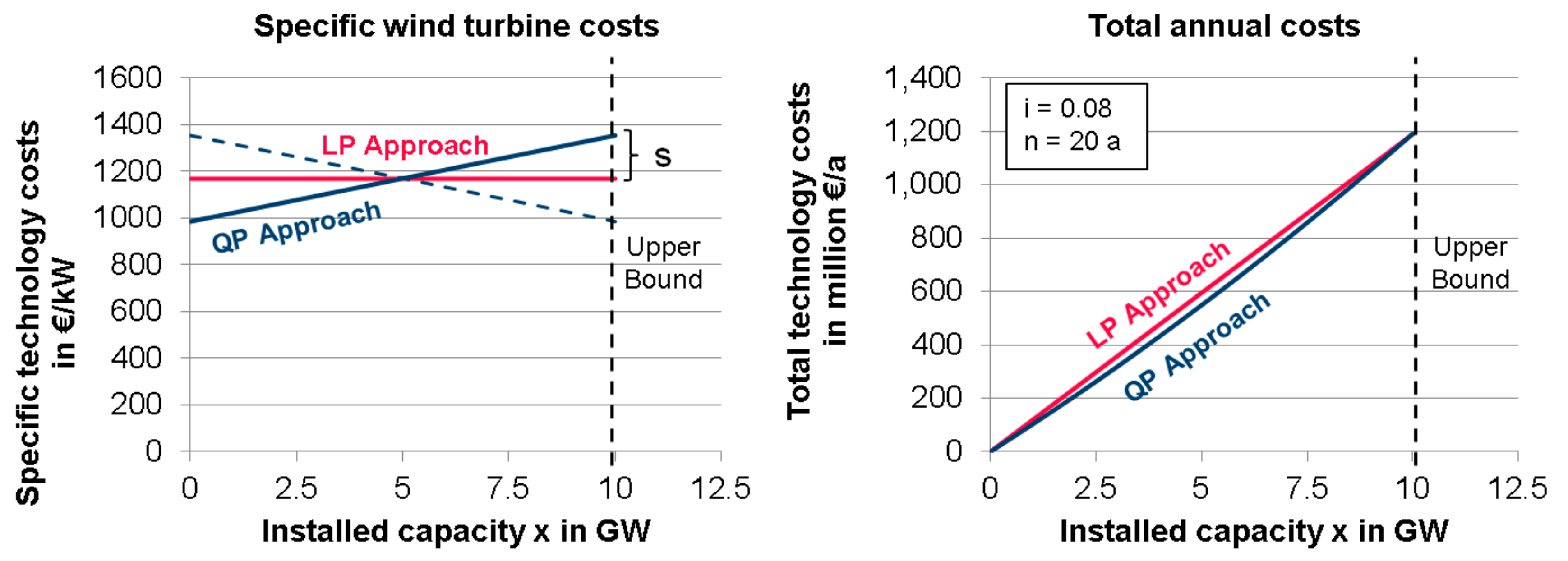
The following approach was developed to overcome the issue of high computational efforts, but still consider the effects of cost ranges in an energy system model. An additional requirement of the approach is that it should be possible to modify existing linear programming models. Therefore, the modified model should be solvable with common solvers, such as Gurobi, CPLEX, or XPRESS. These solvers are only able to handle linear and convex quadratic equations. Due to this limitation, the simplest attempt to integrate cost spans is to define specific costs as linear functions of the model’s dimensioning variables. Consequently, the objective function of the total annual costs becomes quadratic. In Figure 2, both the conventional linear and quadratic approach are compared. While specific costs in linear models equal a constant average value, in the quadratic programming (QP) model, the entire cost range described in the investment cost chapter is distributed over the installable capacity of the technology in a limited period. In this example, it was set to 10 GW. The upper bound of the capacity variable can be either the technical potential of a technology or its expansion limit at a specific time interval. In the depicted case, the cheapest units of the technology were sold first (blue curve). This is supported by the assumption of free markets. In theory, it is also possible to implement the cost range and vice versa (dashed line), for example, to consider learning curves. However, this implicates local optima in the optimization process and a concave objective function, which cannot be solved by the solvers mentioned above. Instead, piecewise linearization can be used for an approximation of this problem and to implement learning curve effects [35]. As mentioned during the investigation of investment costs, the consideration of the uncertainties this paper, targeting and the learning curves effect, do not exclude each other. While learning curve effects occur over long periods, such as decades, the described uncertainty effects are not time-dependent but attributable to a specific construction project. For that reason, the consideration of both effects can be merged in myopic or perfect foresight planning models.
The objective function of the modified linear models is intended to minimize the total annual system costs. These costs are divided into fixed and variable costs. The fixed costs consist of CAPEX and fixed operational expenditures (fixed OPEX) mfix. For the determination of the CAPEX of a specific technology y, the capital recovery factor r is utilized based on interest rate i and the number of periods n (Equation (1)):
In the linear case, the specific technology costs, kLP, are constant and independent of the installed capacity x (Equation (2)). They are based on an average cost value, C0, or a forecasted value for future scenarios. This factor, multiplied by the capital recovery factor and the fixed OPEX as a percentage of C0, results in the fixed costs αLPfix (Equation (3))
Consequently, the total fixed annual costs KLPfix are the integral of αLPfix between the lower xlb and upper bound xub of the capacity of technology y (Equations (4) and (5)):
The variable costs are based on energy and material flows k of the energy system in time step t, which are allocated to the technologies by the ingoing and outgoing flows, . In combination with the total fixed annual costs, the objective function can be expressed, as follows, in Equation (6):
In contrast to the linear approach, the specific cost function of the QP model kQP(xy) has a constant slope v. Moreover, the average cost value C0 can be replaced by the weighted average value in Figure 1. The impact on the fixed costs, αQPfix, is explained in Equations (7)–(9):
Based on these equations, the total fixed annual costs, KQPfix, are described in Equations (10) and (11).
As the declaration of the specific cost slope is not especially common, the equation can be simplified by introducing the absolute deviation s of the minimum or maximum cost value from the average or weighted average cost value (see Figure 2). This leads to Equation (12) for the definition of specific costs kQP. Its consequences to the total fixed annual costs are shown in Equations (13) and (14).
The final objective function of the QP model is shown in Equation (15).
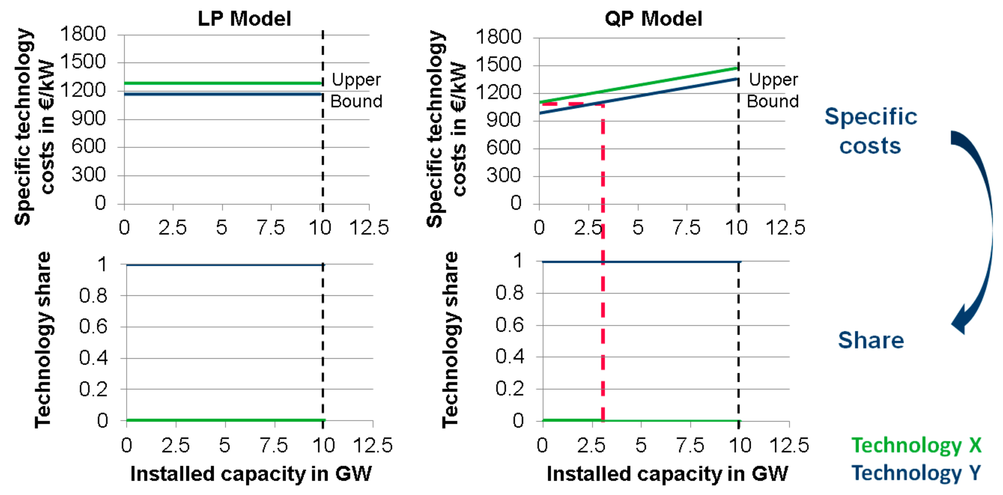
For comparison of the theoretical differences in the results of the LP and QP model, Figure 3 gives a qualitative example of two similar technologies. Both represent options for the supply of the same demand. However, one technology is slightly cheaper than the other. In the linear case, the solver would only decide on the cheaper option. Lowering the specific cost of the more expensive alternative may trigger the penny switching effect and completely change the result. Otherwise, in the QP approach, both technologies would be in the solution if demand is high enough. The closer the specific cost values of the technologies are, the more congruent their shares in the energy system are. As a consequence, the penny switching effect can be avoided, and the results become more robust.
5. Comparison of Linear and Quadratic Programming Results
The corroboration of the hypothesis requires verification through an appropriate testing model. For verification purposes, a linear programming model for minimization of the total energy system costs for Germany was chosen. In this context, a potential energy system for the target year of 2050 was optimized for an 80% CO2 emission reduction scenario, in accordance with the German ‘Klimaschutzplan 2050’ [36]. A detailed description of the model can be found in the methods section.
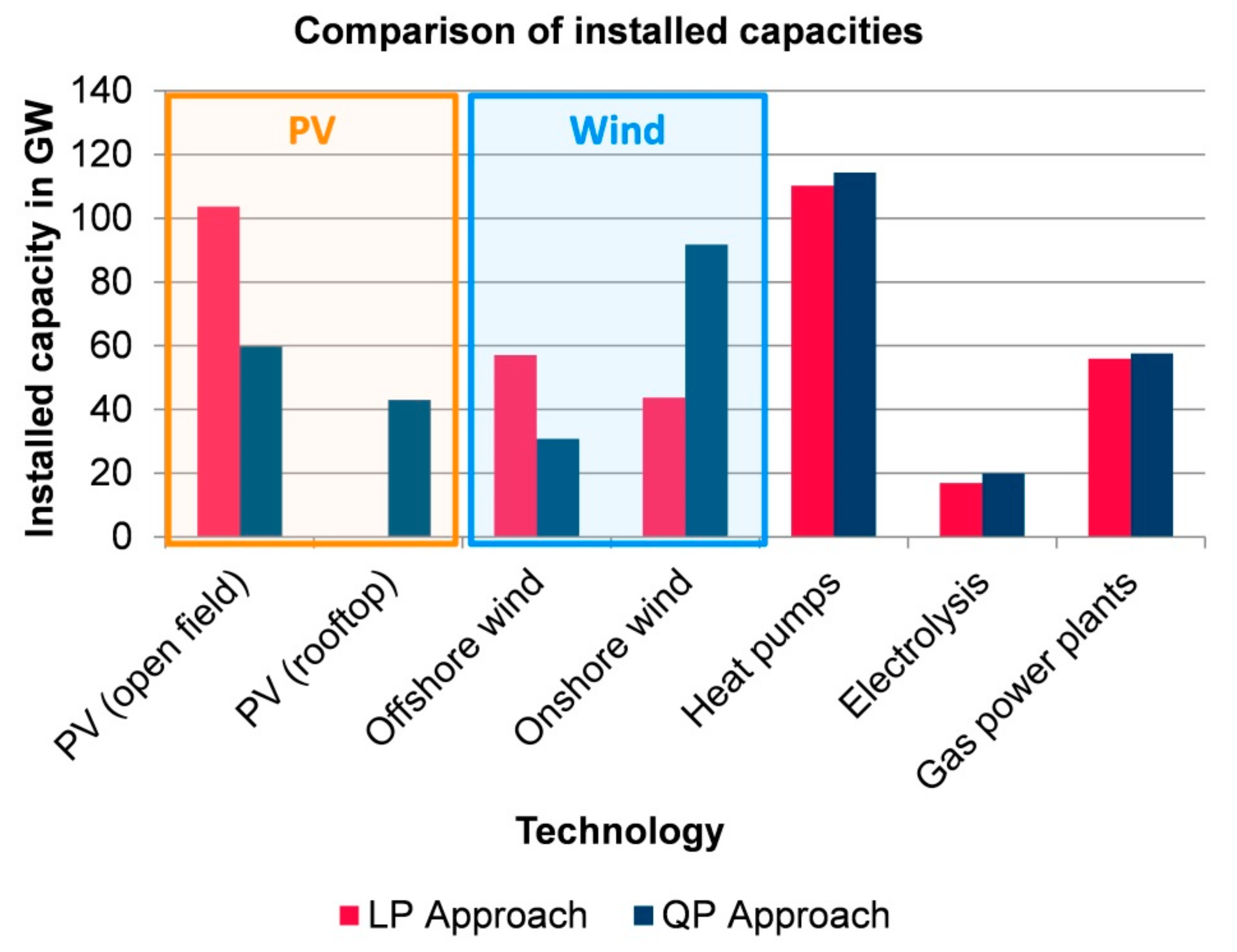
For comparison, the modified testing model was run twice, once with the linear objective function and once with the quadratic objective function. To illustrate the discussed theoretical impact on the results, the focus was on technologies that are sensitive to CAPEX variations. The best example of the penny switching effect is the choice between commercial open field and residential rooftop photovoltaics. Based on the minimal lower total costs of open-field PV [29], linear energy system models tend to expand open-field PV to the edge of its technical potential before building rooftop PV. Another example of this effect is the choice between onshore and offshore wind turbines. Weather and ground conditions in Germany lead to approximately doubled full load hours, accompanied by doubled costs of offshore wind turbines. These effects can be noted in Figure 4. In the linear case (red), the solution considers no rooftop PV and a nearly equal amount of onshore and offshore wind power. Instead, the quadratic case (blue) is represented by a similar share of PV technologies and an increase in onshore wind power. In addition, some other capacities of key technologies of the system are shown and are subject to much smaller changes.
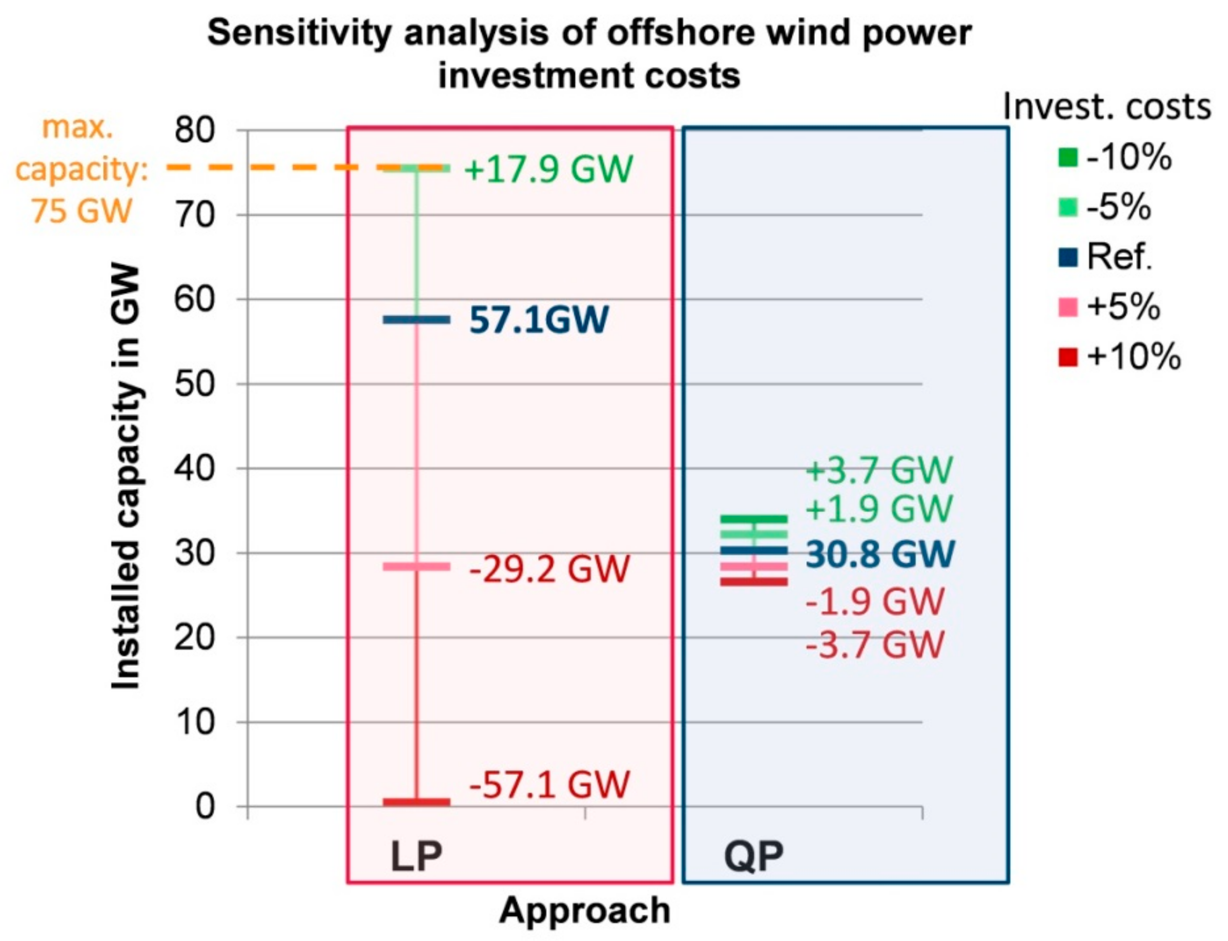
An additional conjecture of the quadratic optimization approach is its impact on the result’s robustness towards variations in the underlying investment cost parameters. For that reason, the results of a sensitivity analysis are shown in Figure 5. This analysis was based on a variation of the offshore wind turbine investment costs by ±10%. In the linear model (marked in red), a massive impact on the installed capacity was registered. The decrease in the investment costs by 5% led to an increase in capacity from 57.1 GW in the reference case (2530 €/kW) up to 75 GW that represents the upper bound in the model (based on the technical potential of offshore wind power in Germany). On the other side, a 10% increase in the costs resulted in the exclusion of offshore wind in the energy system. However, the effect on the capacities was significantly reduced in the QP model, resulting in a range of ±3.7 GW.
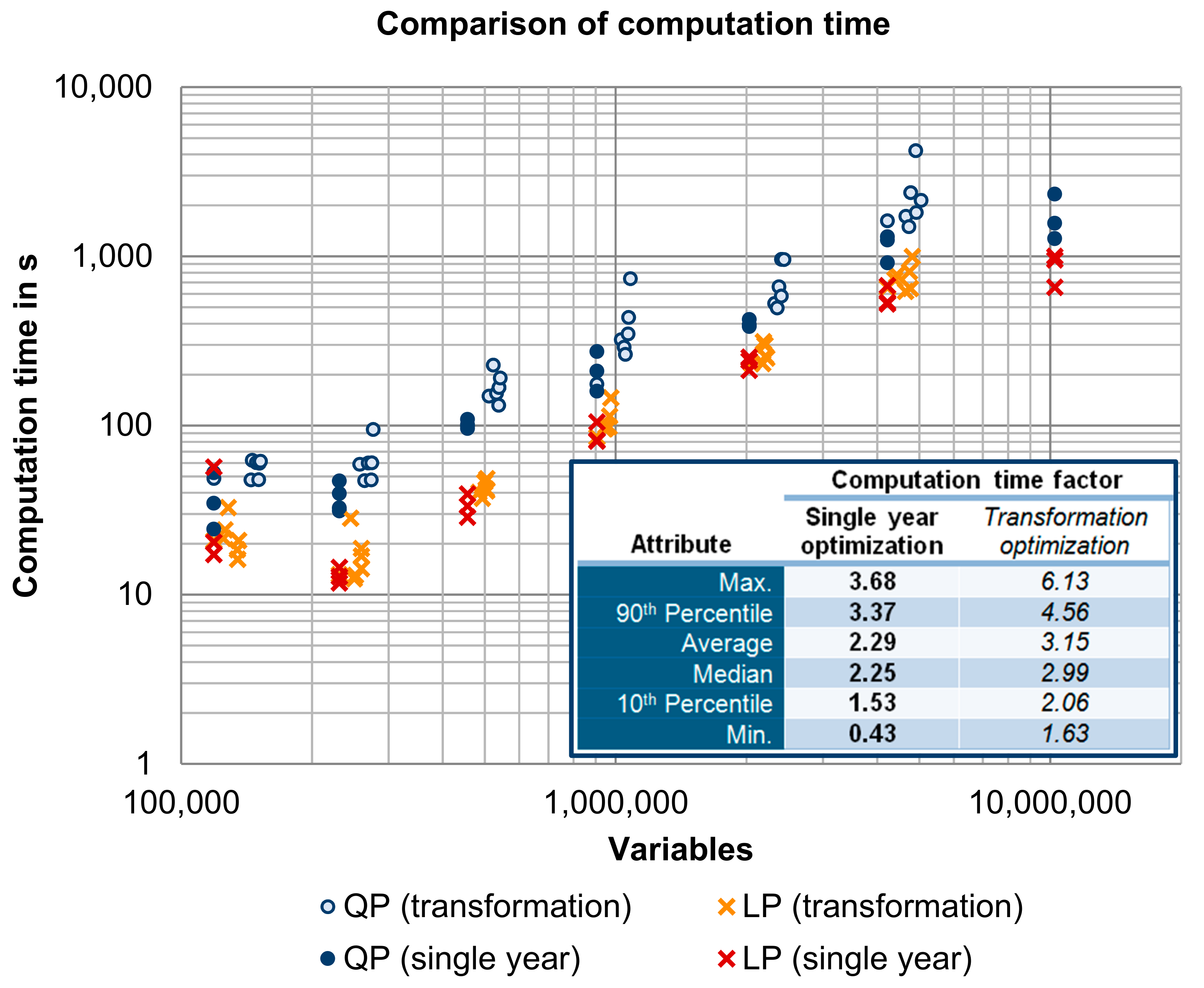
Aside from the impact on the results, it is important to take the changes in computation time using the QP approach into account. Because the computational effort for such complex models is affected by various aspects, the change in computation time is dependent on the individual model, its input parameters, the solver, and its setup. In the case of the model used for verification, the computation time of the QP model was increased by a factor of 2.04 towards the LP model. The optimization was executed by the solver Gurobi. Further investigations with different models and solver setups showed a variation in the computation time by a factor of between 0.43 and 3.68 towards the LP approach for a single year optimization. The average value of the increase in computation time was a factor of 2.29 (median value: 2.25). When it comes to the myopic optimization of an energy system transformation, which is described in the methods section, the QP approach led to a wider range of considered technologies. This effect can be seen in Figure 6 by the increasing number of variables of the QP models compared to the LP models. Consequently, the difference in computation time was further increased by a factor of between 1.63 and 6.13. In total, seven model configurations were analyzed for testing purposes. For each configuration except the most extensive one, three single year optimizations and one transformation assessment based on seven individual optimizations were executed as LP and QP problems. The most extensive model configuration, with more than ten million variables, was only optimized for single years.
6. Discussion and Conclusions
The consideration of uncertainties in energy system models plays a key role in improving the results of these models and the quality of energy scenarios. However, uncertainties range from social to climatological to technical factors. This paper focuses on the uncertainties in the development of technical investment costs. The preceding analysis showed that technological investment costs generally vary across wide ranges, and the predictions of future trends are subject to uncertainties. Nevertheless, these cost ranges can be incorporated and simplified by implementing a quadratic objective function in conventional energy system optimization models. In particular, models to evaluate greenhouse gas reduction strategies that implement high shares of renewable energy in the system benefit from this approach. The investigation reveals that the results of the modified model become more robust, and a broader mix of technologies is considered in the solution. Instead of the penny switching effects in the LP model, the technology shares are affected much less by a variation in the specific investment costs. Moreover, when comparing the results shown in Figure 4 to the current energy system of Germany, the installed capacities of wind power and PV follow actual trends of considered technologies such as rooftop PV. Thus, the solution better reflects the present investment behavior and might be described as more realistic. However, there are two effects of the QP approach that must also be discussed. Concerning the resulting total system costs, the calculated costs of the QP model were systematically lower than in the LP model if the same average value of the investment costs was implemented. This can be attributed to the fact that the average total investment costs of a technology are only equal to the linear case if the installed capacity reaches its upper bound (compare Figure 2). Either this effect is assigned to market behavior and justified by the point of the improved implementation of markets or must be corrected by the real average cost value after optimization. Aside from this effect, the results of the QP model were influenced by the definition of the specific investment cost ranges themselves. This means that the determination of the considered range, as well as the span between the lower and upper bound of installable capacity, affects the result. The wider the cost range and the closer the lower and upper bound, the more the gradient of the specific technology cost curve increased. Consequently, the shares of alternative technologies became more even. This must be taken into consideration when evaluating the results.
In conclusion, the QP or mixed-integer quadratic programming (MIQP) approach to investment costs represents an alternative to cost minimization in conventional LP or mixed-integer linear programming (MILP) models. The results become more robust with respect to cost uncertainties, comprise a wider range of technologies, and sensitivity analyses of cost parameters can be significantly reduced by an acceptably small increase in computation time. Moreover, the approach can be easily implemented in most LP models using solvers such as Gurobi, CPLEX, or XPRESS. Thus, it represents an option for supporting decision-makers in identifying robust key technologies and sensitive pathways in energy systems. Furthermore, the approach can be transferred to any technology in the system. In particular, the implementation of energy efficiency measures and end-use technologies, as well as in the transport and industry sector in general, has high potential to gain new insights. This should be further investigated, also to validate the presented results by other models and technologies in the future.
Author Contributions
Conceptualization, P.L.; methodology, P.L.; writing—original draft preparation, P.L.; writing—review and editing, P.M., D.S., and M.R.; supervision, P.M., M.R., and D.S.
Funding
This research received no external funding.
Conflicts of Interest
The authors declare no conflict of interest.
Appendix A

| Component | Specific Invest. Costs in €/kW | Cost Range in Percentage Deviation | Level of Efficiency | CO2 Emissions in gCO2/kWh | ||||
|---|---|---|---|---|---|---|---|---|
| Name | Today | 2050 | Today | 2050 | Today | 2050 | Today | 2050 |
| Photovoltaics (rooftop) | 1500 | 880 | ±23% | ±14% | (1) * | (1) * | 0 | 0 |
| Photovoltaics (open field) | 1100 | 720 | ±9% | ±11% | (1) * | (1) * | 0 | 0 |
| Onshore wind power | 1850 | 1250 | ±30% | ±36% | (1) * | (1) * | 0 | 0 |
| Offshore wind power | 3920 | 2530 | ±21% | ±29% | (1) * | (1) * | 0 | 0 |
| Coal power station | 1600 | 1600 | ±9% | ±9% | 0.45 | 0.48 | 890 | 840 |
| Lignite power station | 2050 | 2050 | ±17% | ±17% | 0.42 | 0.47 | 1010 | 910 |
| Gas power station | 550 | 550 | ±27% | ±27% | 0.40 | 0.45 | 575 | 510 |
| Biomass power station | 3200 | 2080 | ±22% | ±21% | 0.34 | 0.38 | (0) ** | (0) ** |
| Hydropower station | 5250 | 5370 | ±52% | ±52% | (1) * | (1) * | 0 | 0 |
| Pumped hydro storage | 3000 | 3000 | ±50% | ±50% | 0.8 *** | 0.9 *** | 0 | 0 |
| Battery storage (Li) | 752 (€/kWh) | 246 (€/kWh) | ±20% | ±20% | 0.9 *** | 0.9 *** | 0 | 0 |
| Hydrogen cavern storage | 0.52 (€/kWh) | 0.52 (€/kWh) | ±0% | ±0% | 1 | 1 | 0 | 0 |
| Electrolyzer (PEM) | 1564 | 500 | ±21% | ±21% | 0.69 | 0.7 | 0 | 0 |
| Fuel cell (PEM) | 3650 | 923 | ±4% | ±4% | 0.49 | 0.5 | 0 | 0 |
| Heat pumps | 800 (€/kWel) | 645 (€/kWel) | ±38% | ±38% | 3.0 (COP) | 3.5 (COP) | 0 | 0 |
The model’s structure and parameters were validated based on historical data from the year 2013 in accordance with the integrated supply and demand profiles.
References
- Lopion, P.; Markewitz, P.; Robinius, M.; Stolten, D. A Review of Current Challenges and Trends in Energy Systems Modeling. Renew. Sustain. Energy Rev. 2018, 96, 156–166. [Google Scholar] [CrossRef]
- Van Beeck, N. Classification of Energy Models; Tilburg University, Faculty of Economics and Business Administration: Tilburg, The Netherlands, 2000. [Google Scholar]
- Hall, L.M.; Buckley, A.R. A Review of Energy Systems Models in the UK: Prevalent Usage and Categorisation. Appl. Energy 2016, 169, 607–628. [Google Scholar] [CrossRef]
- Pfenninger, S.; Hawkes, A.; Keirstead, J. Energy Systems Modeling for Twenty-First Century Energy Challenges. Renew. Sustain. Energy Rev. 2014, 33, 74–86. [Google Scholar] [CrossRef]
- Anadon, L.D.; Baker, E.; Bosetti, V. Integrating Uncertainty into Public Energy Research and Development Decisions. Nat. Energy 2017, 2, 17071. [Google Scholar] [CrossRef]
- Ma, T.; Nakamori, Y. Modeling Technological Change in Energy Systems–From Optimization to Agent-Based Modeling. Energy 2009, 34, 873–879. [Google Scholar] [CrossRef]
- Mccollum, D.L.; Zhou, W.; Bertram, C.; De Boer, H.S.; Bosetti, V.; Busch, S.; Despres, J.; Drouet, L.; Emmerling, J.; Fay, M.; et al. Author Correction: Energy Investment Needs for Fulfilling the Paris Agreement and Achieving the Sustainable Development Goals. Nat. Energy 2018, 3, 699. [Google Scholar] [CrossRef]
- Winskel, M. Beyond the Disruption Narrative: Varieties and Ambiguities of Energy System Change. Energy Res. Soc. Sci. 2018, 37, 232–237. [Google Scholar] [CrossRef]
- Tattini, J.; Gargiulo, M.; Karlsson, K. Reaching Carbon Neutral Transport Sector in Denmark–Evidence from the Incorporation of Modal Shift into the TIMES Energy System Modeling Framework. Energy Policy 2018, 113, 571–583. [Google Scholar] [CrossRef]
- Tattini, J.; Ramea, K.; Gargiulo, M.; Yang, C.; Mulholland, E.; Yeh, S.; Karlsson, K. Improving the Representation of Modal Choice into Bottom-Up Optimization Energy System Models–The MoCho-TIMES Model. Appl. Energy 2018, 212, 265–282. [Google Scholar] [CrossRef]
- Gritsevskyi, A.; Nakicenovi, N. Modeling Uncertainty of Induced Technological Change. Energy Policy 2000, 28, 907–921. [Google Scholar] [CrossRef]
- Schmidt, O.; Hawkes, A.; Gambhir, A.; Staffell, I. The Future Cost of Electrical Energy Storage Based on Experience Rates. Nat. Energy 2017, 2, 17110. [Google Scholar] [CrossRef]
- Held, A.M. Modelling the Future Development of Renewable Energy Technologies in the European Electricity Sector Using Agent-Based Simulation; Fraunhofer Verlag: Stuttgart, Germany, 2011. [Google Scholar]
- Kovacevic, R.M.; Pflug, G.C.; Vespucci, M.T. Handbook of Risk Management in Energy Production and Trading; Springer: Boston, MA, USA, 2013. [Google Scholar]
- Pfluger, B. Assessment of Least-Cost Pathways for Decarbonising Europe’s Power Supply: A Model-Based Long-Term Scenario Analysis Accounting for the Characteristics of Renewable Energies; KIT Scientific Publishing: Karlsruhe, Germany, 2014. [Google Scholar]
- Connolly, D.; Lund, H.; Mathiesen, B.V.; Leahy, M. A Review of Computer Tools for Analysing the Integration of Renewable Energy into Various Energy Systems. Appl. Energy 2010, 87, 1059–1082. [Google Scholar] [CrossRef]
- Bosetti, V.; Marangoni, G.; Borgonovo, E.; Anadon, L.D.; Barron, R.; McJeon, H.C.; Politis, S.; Friley, P. Sensitivity to Energy Technology Costs: A Multi-Model Comparison Analysis. Energy Policy 2015, 80, 244–263. [Google Scholar] [CrossRef]
- Seljom, P.; Tomasgard, A. Short-Term Uncertainty in Long-Term Energy System Models—A Case Study of Wind Power in Denmark. Energy Econ. 2015, 49, 157–167. [Google Scholar] [CrossRef]
- Welder, L.; Ryberg, D.; Kotzur, L.; Grube, T.; Robinius, M.; Stolten, D. Spatio-Temporal Optimization of a Future Energy System for Power-To-Hydrogen Applications in Germany. Energy 2018, 158, 1130–1149. [Google Scholar] [CrossRef]
- Kotzur, L.; Markewitz, P.; Robinius, M.; Stolten, D. Time Series Aggregation for Energy System Design: Modeling Seasonal Storage. arXiv 2017, arXiv:171007593. [Google Scholar] [CrossRef]
- Kotzur, L.; Markewitz, P.; Robinius, M.; Stolten, D. Impact of Different Time Series Aggregation Methods on Optimal Energy System Design. Renew. Energy 2018, 117, 474–487. [Google Scholar] [CrossRef]
- Burger, V.; Hesse, T.; Quack, D.; Palzer, A.; Kohler, B.; Herkel, S.; Engelmann, P. Klimaneutraler Gebaudebestand 2050; the German Environment Agency Climate Change: Dessau-Rosslau, Germany, 2016; Volume 6, p. 2016. [Google Scholar]
- Gerbert, P.; Herhold, P.; Burchardt, J.; Schonberger, S.; Rechenmacher, F.; Kirchner, A.; Kemmler, A.; Wünsch, M. Klimapfade Fur Deutschland; Bundesverbandes Der Deutschen Industrie (BDI): Berlin, Germany, 2018. [Google Scholar]
- IRENA. Renewable Power Generation Costs in 2017; International Renewable Energy Agency: Abu Dhabi, Arab, 2018. [Google Scholar]
- Drechsler, M.; Egerer, J.; Lange, M.; Masurowski, F.; Meyerhoff, J.; Oehlmann, M. Efficient and Equitable Spatial Allocation of Renewable Power Plants at the Country Scale. Nat. Energy 2017, 2, 17124. [Google Scholar] [CrossRef]
- Afanasyeva, S.; Saari, J.; Kalkofen, M.; Partanen, J.; Pyrhonen, O. Technical, Economic and Uncertainty Modelling of a Wind Farm Project. Energy Convers. Manag. 2016, 107, 22–33. [Google Scholar] [CrossRef]
- Rout, U.K.; Blesl, M.; Fahl, U.; Remme, U.; Vois, A. Uncertainty in the Learning Rates of Energy Technologies: An Experiment in a Global Multi-Regional Energy System Model. Energy Policy 2009, 37, 4927–4942. [Google Scholar] [CrossRef]
- Moccia, J.; Arapogianni, A.; Wilkes, J.; Kjaer, C.; Gruet, R.; Azau, S.; Scola, J. Pure Power-Wind Energy Targets for 2020 and 2030; Ewea; European Wind Energy Association: Brussels, Belgium, 2011. [Google Scholar]
- Carlsson, J. Energy Technology Reference Indicator Projections for 2010–2050; European Commission, Joint Research Centre, Institute for Energy and Transport Luxembourg: Peten, The Netherlands; Ispra, Italy, 2014. [Google Scholar]
- Roadmap, E. 2050: A Practical Guide to a Prosperous, Low Carbon Europe; ECF: Brussels, Belgium, 2010. [Google Scholar]
- Taylor, M.; Ralon, P.; Ilas, A. The Power to Change: Solar and Wind Cost Reduction Potential to 2025; International Renewable Energy Agency (IRENA): Abu Dhabi, Arab, 2016. [Google Scholar]
- MacDonald, M. Costs of Low-Carbon Generation Technologies, Report for the Committee on Climate Change Brighton, Mott MacDonald; The Committee on Climate Change Brighton: Brighton, UK, 2011. [Google Scholar]
- Creutzig, F.; Agoston, P.; Goldschmidt, J.C.; Luderer, G.; Nemet, G.; Pietzcker, R.C. The Underestimated Potential of Solar Energy to Mitigate Climate Change. Nat. Energy 2017, 2, 17140. [Google Scholar] [CrossRef]
- Mccollum, D.L.; Jewell, J.; Krey, V.; Bazilian, M.; Fay, M.; Riahi, K. Quantifying Uncertainties Influencing the Long-Term Impacts of Oil Prices on Energy Markets and Carbon Emissions. Nat. Energy 2016, 1, 16077. [Google Scholar] [CrossRef]
- Heuberger, C.F.; Rubin, E.S.; Staffell, I.; Shah, N.; Mac Dowell, N. Power Capacity Expansion Planning Considering Endogenous Technology Cost Learning. Appl. Energy 2017, 204, 831–845. [Google Scholar] [CrossRef]
- Bundesministerium Fur Umwelt N, Bau und Reaktorsicherheit. Klimaschutzplan 2050–Klimapolitische Grundsatze und Ziele der Bundesregierung; Bundesministerium Fur Umwelt: Berlin, Germany, 2016. [Google Scholar]
- Saba, S.M.; Muller, M.; Robinius, M.; Stolten, D. The Investment Costs of Electrolysis–A Comparison of Cost Studies from the Past 30 Years. Int. J. Hydrog. Energy 2018, 43, 1209–1223. [Google Scholar] [CrossRef]
- Noack, C.; Burggraf, F.; Hosseiny, S.; Lettenmeier, P.; Kolb, S.; Belz, S.; Kallo, J.; Friedrich, A.; Pregger, T.; Cao, K.; et al. Studie Uber Die Planung Einer Demonstrationsanlage Zur Wasserstoff-Kraftstoffgewinnung Durch Elektrolyse Mit Zwischenspeicherung in Salzkavernen Unter Druck; German Aerospace Center: Stuttgart, Germany, 2015. [Google Scholar]
- Stolzenburg, K.; Hamelmann, R.; Wietschel, M.; Genoese, F.; Michaelis, J.; Lehmann, J.; Miege, A.; Krause, S.; Sponholz, C.; Donadei, S.; et al. Integration Von Wind-Wasserstoff-Systemen in Das Energiesystem. Analysis on Behalf of Nationale Organisation Wasserstoff-Und Brennstoffzellentechnologie GmbH (NOW); NOW: Berlin, Germany, 2014. [Google Scholar]
- AGEB. Energiebilanzen 1990-2016; AGEB: Berlin, Germany, 1990. [Google Scholar]
- Harthan, R.O.; Hermann, H. Sektorale Abgrenzung Der Deutschen Treibhausgasemissionen Mit Einem Schwerpunkt Auf Die Verbrennungsbedingten CO2-Emissionen; Oko-Institut eV: Berlin, Geremany, 2018. [Google Scholar]
Figure 1.
Investment cost range and deviations of onshore wind turbines, based on the IRENA (International Renewable Energy Agency) renewable cost database [24].
Figure 1.
Investment cost range and deviations of onshore wind turbines, based on the IRENA (International Renewable Energy Agency) renewable cost database [24].

Figure 2.
Comparison of the consideration of investment costs in the linear programming (LP) (red) and quadratic programming (QP) model (blue).
Figure 2.
Comparison of the consideration of investment costs in the linear programming (LP) (red) and quadratic programming (QP) model (blue).

Figure 3.
Qualitative comparison of two similar technology shares in the optimized solution of the LP and QP model.
Figure 3.
Qualitative comparison of two similar technology shares in the optimized solution of the LP and QP model.

Figure 4.
Comparison of installed capacities in the results of the LP (red) and QP (blue) model for an 80% CO2 emission reduction scenario for Germany.
Figure 4.
Comparison of installed capacities in the results of the LP (red) and QP (blue) model for an 80% CO2 emission reduction scenario for Germany.

Figure 5.
Sensitivity analysis of the investment costs for offshore wind turbines and its impact on the installed capacity in the cost-optimized energy system in the LP and QP model.
Figure 5.
Sensitivity analysis of the investment costs for offshore wind turbines and its impact on the installed capacity in the cost-optimized energy system in the LP and QP model.

Figure 6.
Comparison of computation time of different LP and QP problems.

© 2019 by the authors. Licensee MDPI, Basel, Switzerland. This article is an open access article distributed under the terms and conditions of the Creative Commons Attribution (CC BY) license (http://creativecommons.org/licenses/by/4.0/).
Share and Cite
MDPI and ACS Style
Lopion, P.; Markewitz, P.; Stolten, D.; Robinius, M. Cost Uncertainties in Energy System Optimization Models: A Quadratic Programming Approach for Avoiding Penny Switching Effects. Energies 2019, 12, 4006. https://doi.org/10.3390/en12204006
AMA Style
Lopion P, Markewitz P, Stolten D, Robinius M. Cost Uncertainties in Energy System Optimization Models: A Quadratic Programming Approach for Avoiding Penny Switching Effects. Energies. 2019; 12(20):4006. https://doi.org/10.3390/en12204006
Chicago/Turabian StyleLopion, Peter, Peter Markewitz, Detlef Stolten, and Martin Robinius. 2019. "Cost Uncertainties in Energy System Optimization Models: A Quadratic Programming Approach for Avoiding Penny Switching Effects" Energies 12, no. 20: 4006. https://doi.org/10.3390/en12204006
Note that from the first issue of 2016, this journal uses article numbers instead of page numbers. See further details here.