A Multi-Scale Analysis of the Fire Problems in an Urban Utility Tunnel

Abstract

Building utility tunnels has been widely adopted as an important solution for the sustainable development of cities, but their unique fire problems have not attracted enough attention to date. With the purpose of preliminarily understanding the fire phenomena in a utility tunnel, this study performed a comprehensive analysis, including the burning behaviour of accommodated cables, hot gas temperature field and enhanced fuel burning rates based on bench-scale, full-scale and model-scale fire tests. The critical exposed radiative heat flux for the 10-kV power cable to achieve complete burning was identified. The whole burning process was divided into five phases. The cable’s noteworthy hazards and dangerous fire behaviours were also examined. The two-dimensional (2D) gas temperature fields and longitudinal maximum temperature distributions were investigated carefully, after which a versatile model was derived. The model predicted the maximum temperature attenuation of both upstream and downstream flows reasonably well. Finally, the phenomenon of enhanced fuel burning was explored. A multivariate cubic function that considers the global effects of relative width, height and distance was further proposed to estimate the enhancement coefficient. The current findings can provide designers and operators with valuable guidance for the integrated promotion of utility tunnels’ fire safety level.

1. Introduction

Urban utility tunnels are joint-use underground passages for accommodating multiple utilities such as water, sewerage, gas, electrical power, telephone and heat supply. Currently, for sustainable development, building these tunnels has been regarded as a problem-solving technique in more and more countries [1,2]. Alongside this rapid development, catastrophic tunnel fire incidents have motivated abundant research, and their systematic reviews have been well presented in two professional books [3,4], both with a focus on transportation-related tunnels. However, the new utility tunnel fire problems have not yet attracted enough attention, despite a few case studies [5,6].

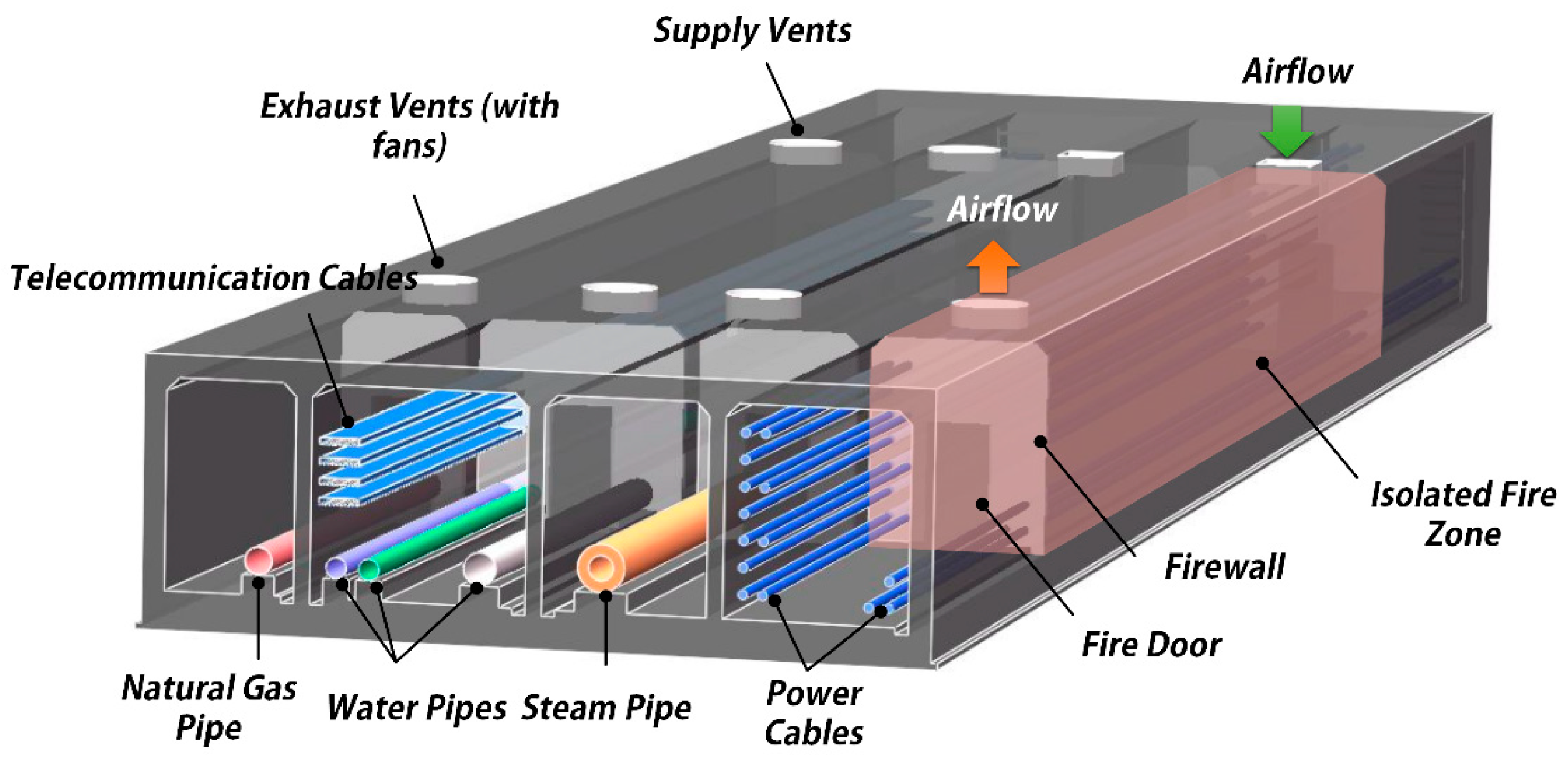
Meanwhile, it is challenging to apply the findings from traffic tunnel research. Figure 1 illustrates a typical cast-in-situ utility tunnel. Normally, the tunnel itself is divided into three or four compartments to accommodate pipelines with different hazard levels. Each compartment contains fire-rated walls and doors to set isolated zones. Conversely, traffic tunnels are always unobstructed at both ends and often for much longer. It is also noteworthy that cables arranged on trays, once ignited, are more likely to spread than vehicles. Moreover, rather than continuously controlling smoke to facilitate safe evacuation [3,4], the ventilation systems are expected to guarantee the safety of pipelines, fire fighters and structures in a utility tunnel. Isolated fire zones also provide the possibility of suffocating the fire spread. Accordingly, the tunnel geometry, fuel packages and ventilation systems of a utility tunnel fundamentally differ from those of a traffic tunnel. This will bring about very different fire problems.

The burning behaviour of cables has been attractive for a long time. Abundant tests have been conducted by the Factory Mutual Research Corporation (FMRC) [7] and European Commission [8]. Recently, two other large projects, the CAROLFIRE (Cable Response to Live Fire) [9] and CHRISTIFIRE (Cable Heat Release, Ignition, and Spread in Tray Installations During Fire) [10,11], were conducted by the U.S. Nuclear Regulatory Commission. Electrical failure mechanisms were investigated and tools for the prediction of the failure were improved. The CHRISTIFIRE project further quantified the burning characteristics of a wide range of cables installed in horizontal trays and vertical trays and developed a model to estimate the flame spread and heat release rate (HRR). In these projects, the tested cables were actually small in terms of their dimensions, while cables that run along a utility tunnel are much larger and loaded with a high voltage from 10 kV to 220 kV. The burning characteristics of these cables thus could be very different. Unfortunately, only a few tests on similar cables used in nuclear power plants [12,13] could be found.

On the other hand, the gas temperature field generated by fires in tunnel structures has been explored by many researchers. Primary studies started from those under a beamed ceiling [14]. Later, Hu et al. [15,16] developed a simple exponential function to predict the longitudinal decay of average gas temperature based on full-scale fire tests in a road tunnel. To predict the maximum temperature decay, Ingason and Li [17] performed a detailed comparison of test results, including model-scale tests, the Runehamar tests and Memorial tests, and finally suggested a well-known empirical equation that was validated under longitudinal ventilation. Nonetheless, most of these equations were established in the context of road tunnels with both ends open. Furthermore, the height of fire source was rarely changed in these studies, but this should be possible in scenarios as a fire can occur at a high position on the cable tray.

Another very hazardous phenomenon should also be noted—the same fuel burning in tunnels would lead to a much higher heat release rate compared with the similar fuel burning in an open space. Carvel et al. [18] made a comprehensive review of documented tunnel fire tests, identified the most influential factor $\frac{W_F}{W_T}$ (the ratio of fuel pan width to tunnel width) based on Bayesian methodology and proposed a polynomial function to assess the enhancement coefficient $\Psi$. In contrast, researchers at SP Technical Research Institute of Sweden [19,20] also conducted model-scale fire tests, but came to the conclusion that the tunnel height has a larger influence on enhanced HRR for pool fires. Apart from this discrepancy, whether the closed tunnel end has an effect or not is still unknown.

The current work presents a multi-scale analysis of the fire problems in an urban utility tunnel. More specifically, bench-scale tests to inspect the burning behaviour of cables, full-scale tests to investigate the gas temperature field and model-scale tests to examine the enhanced burning rate of fuels were all performed, with the purpose being to preliminarily understand the fire phenomena in a utility tunnel. This research can provide designers and operators with valuable guidance for the integrated promotion of utility tunnels’ fire safety level, in order to guarantee a sustainable future.

2. Experimental Method

2.1. Bench-Scale Tests

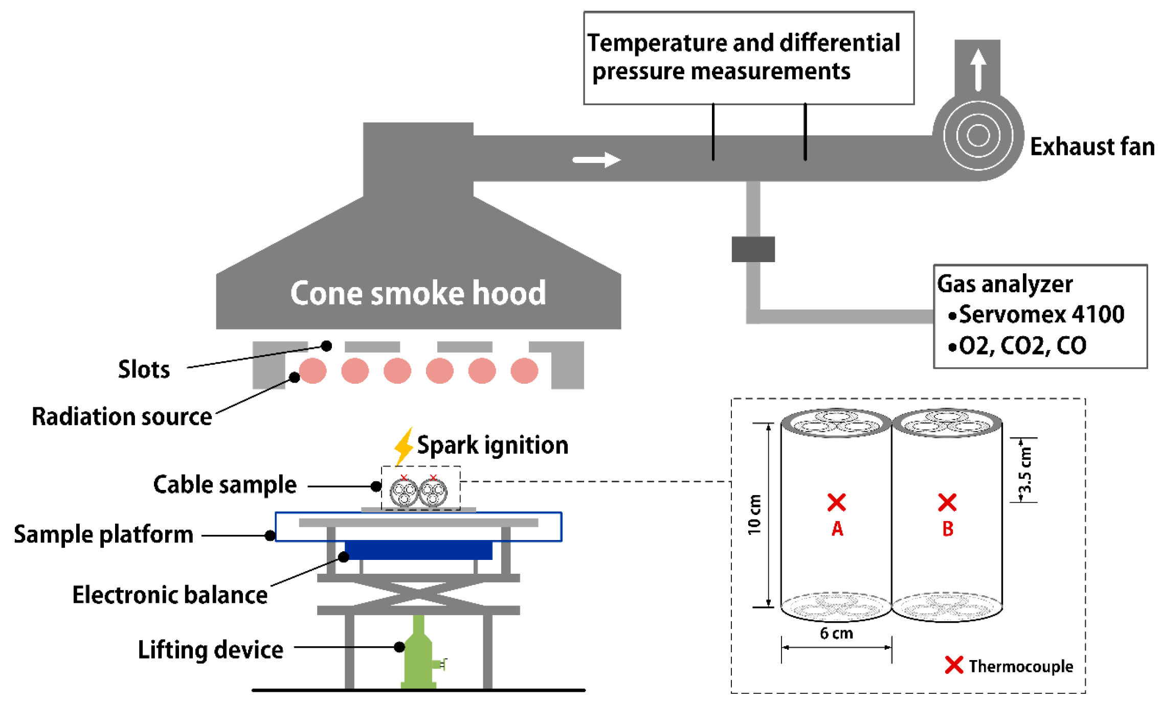
A schematic diagram of the calorimeter apparatus for testing the high-voltage cables is shown in Figure 2. The radiation source was made of 18 silicon carbide rods, which could supply a uniform radiative heat flux of up to 50 kW/m². Slots were set above so that the pyrolysis volatiles or smoke could pass and be collected through the cone hood with an exhaust fan. In the gas duct, both differential pressure and temperature variances were measured by a bidirectional probe and a thermocouple, respectively. A Servomex 4100 gas analyser was also set to test the concentration of oxygen, carbon dioxide and carbon monoxide. Cable samples were placed in the middle on a fireproof quartz stone slab whose dimensions were 30 cm (length) × 18 cm (width) × 2 cm (thickness). Before each test, the slab was replaced. The central location of the cables under the radiation source was ensured. A spark was used for their piloted ignition. The mass of the cables was measured by an electronic balance. The whole burning process was recorded by a video camera. The HRR of burning cables could further be calculated on the basis of the oxygen consumption principle [21] and ISO 5660 [22].

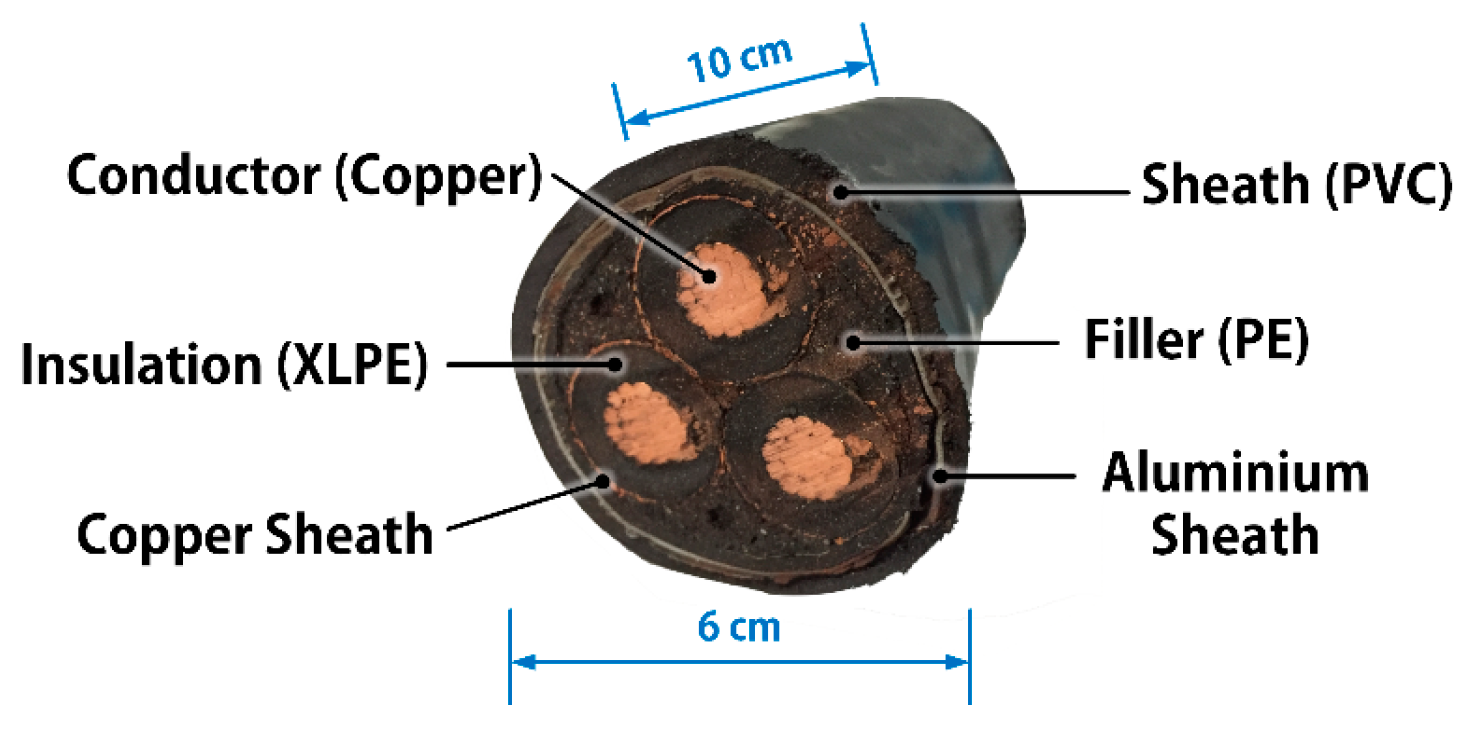
The tested cable, the ZRC-YJV-8.7/10 3 × 95 mm² power cable, was a common type of 10 kV flame retardant cable installed in Chinese utility tunnels. As shown in Figure 3, the main components were PVC (Polyvinyl chloride) sheath, PE (Polyethylene) filler, XLPE (Cross-linked polyethylene) insulation and copper as the conductor. The filler and insulation were also cladded with aluminium binding and copper binding, respectively. The cable sample had a rough diameter of 6 cm and a length of 10 cm. In the tests, two cable samples were adjoining and roughly occupied an area of 10 cm × 12 cm. This meant that the exposed area of the samples to the radiation source was about $60\mathsf{\pi }$ cm². Two thermocouples were fixed on the surface of the two cables, respectively. Their positions could be seen in Figure 2. Two tests were carried out under the radiative heat flux of 24.9 kW/m² and 28.3 kW/m², respectively.

2.2. Full-Scale Tests

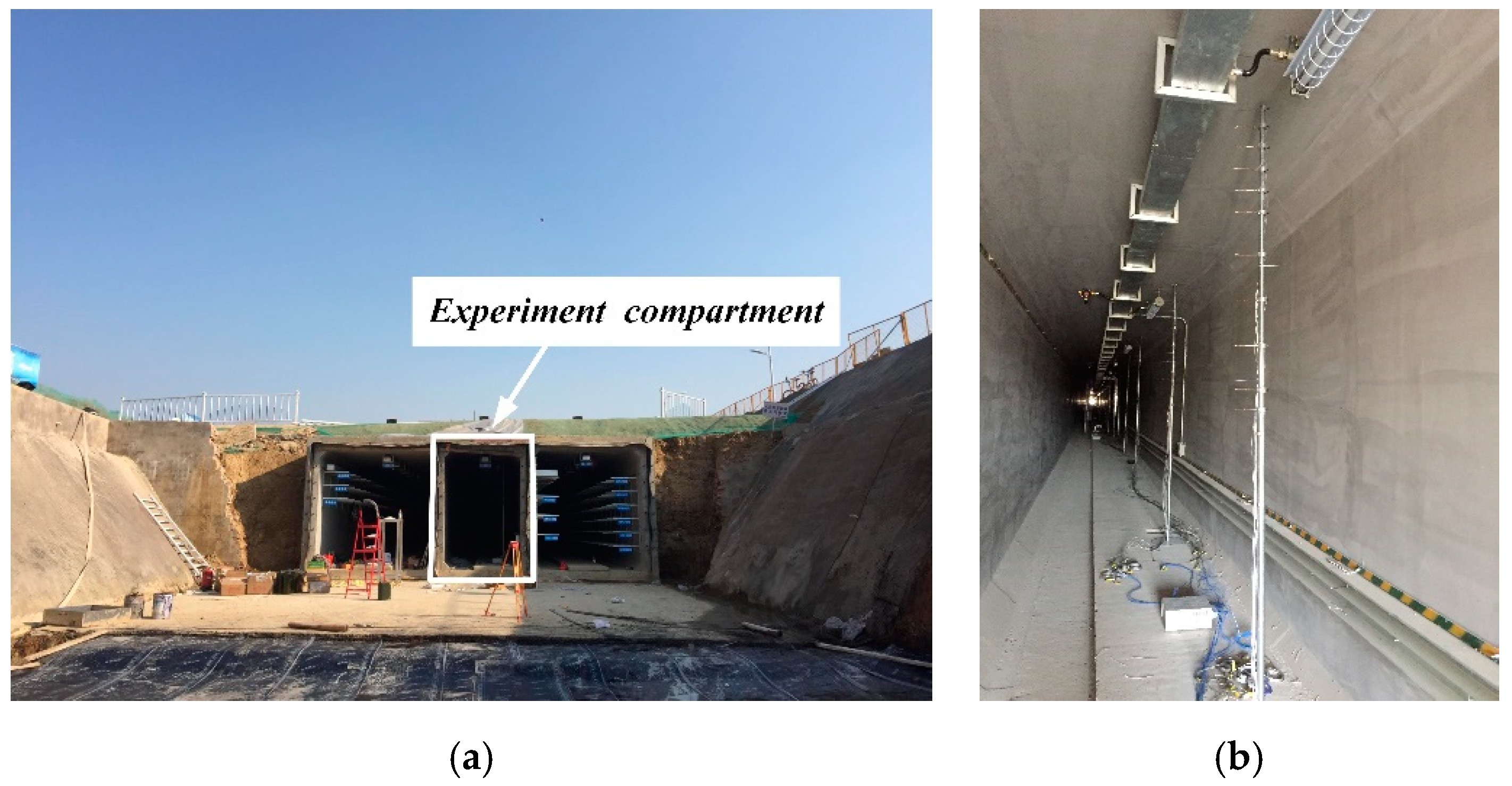
A series of full-scale experiments were also conducted in a cast-in-site utility tunnel under construction in China, as shown in Figure 4. Nine tests were performed in the middle compartment, whose dimensions were 81 m (length) × 2 m (width) × 3 m (height). The east portal of the compartment was fully-closed while the west was totally open. The cross section was a chamfering rectangle with a 10 cm thick flat floor near the sidewall. There were only a few facilities in it, including one enclosed cable tray beneath the ceiling and some daylight lamps, as shown in Figure 4b. There were no openings or ventilation equipment in the test compartment.

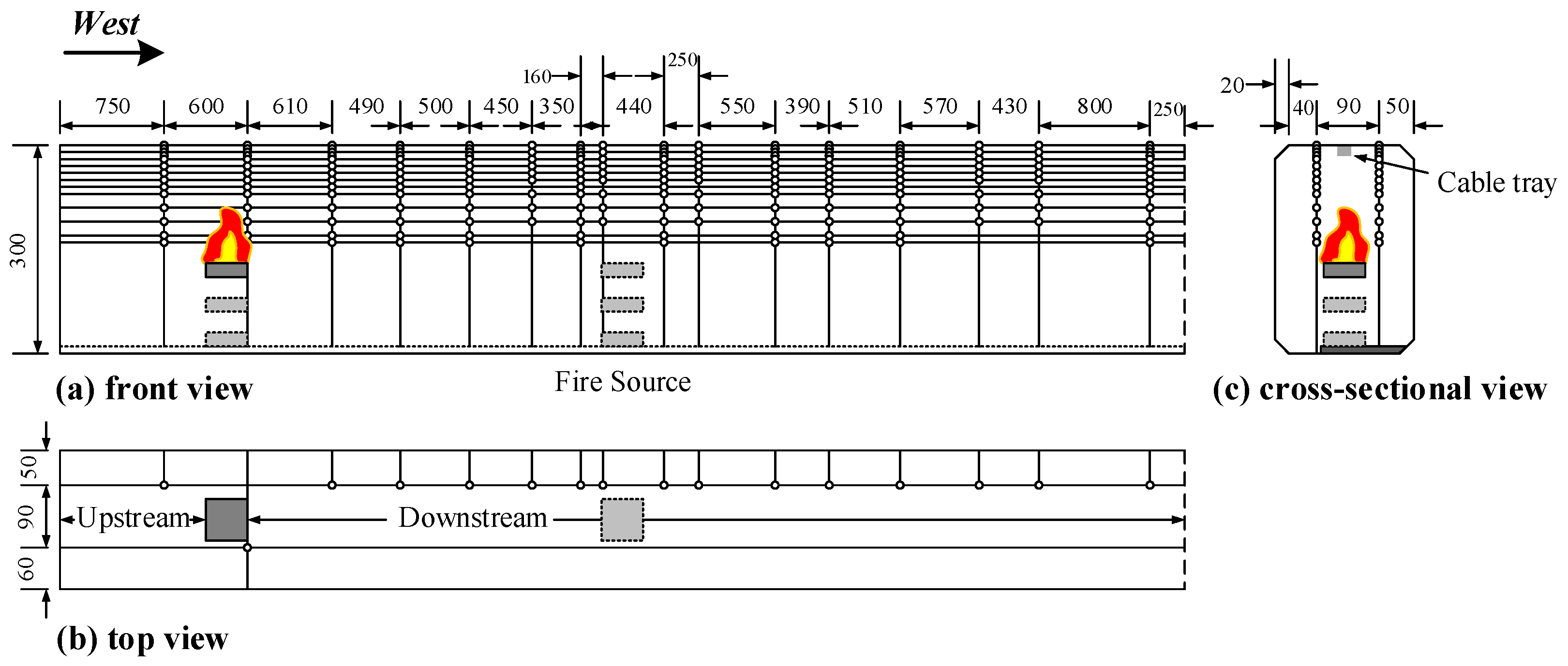
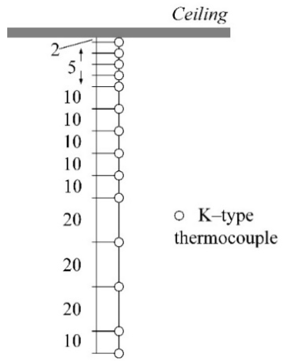
To precisely record the gas temperature field, a total of 16 piles of K-type thermocouple (strand wire diameter of 0.1 mm) were set along the longitudinal direction, as shown in Figure 5. All the piles were placed 50 cm from one sidewall, except one with 60 cm from the other. The temperature distributions were obtained at 7.5, 13.5, 19.6, 24.5, 29.5, 34, 37.5, 40.5 (changed to 39.1 m in Test C01-03), 43.5, 46, 51.5, 55.4, 60.5, 66.2, 70.5 and 78.5 m from the east end wall. For most piles, 14 vertical positions were included (Figure 6). Piles at 34, 40.5 (or 39.1), 46, 66.2 and 70.5 m from the east end did not include the positions of 0.07, 0.17, 0.62, 1.32 and 1.42 m vertically.

During Test S01, fire-retardant fabric was used to fully close the west end in order to form an enclosed space. In the other tests, the west end was open completely. Heptane pool fire was employed as the fire source, while diesel was employed for the enclosed case. The fuel pan had two sizes and was placed in the middle transversely. Horizontally, the fire sources were set at 12 m or 40.5 m (middle) away from the east end. As mentioned, a fire can occur at a high position on the cable tray in utility tunnels. Consequently, the fire source was changed to three vertical locations to simulate these conditions. All the tests were summarized in

Table 1. Summary of the full-scale and model-scale tests.

Test No.	Ambient Temperature T∞ (°C)	Fuel Type	Fuel Pan Size (cm × cm × cm)	Horizontal Distance from East End (m)	Ceiling Clearance, H (m)	East End	West End
E01	13.5	Heptane	40 × 40 × 20	12	2.9	Closed	Open
E02	13.3	Heptane	60 × 60 × 20	12	2.9	Closed	Open
E03	11.9	Heptane	60 × 60 × 20	12	2.9	Closed	Open
E04	12.6	Heptane	60 × 60 × 20	12	2.4	Closed	Open
E05	13.0	Heptane	60 × 60 × 20	12	1.9	Closed	Open
C01	13.3	Heptane	60 × 60 × 20	40.5	2.9	Closed	Open
C02	14.3	Heptane	60 × 60 × 20	40.5	2.4	Closed	Open
C03	15.1	Heptane	60 × 60 × 20	40.5	1.9	Closed	Open
S01	13.8	Diesel	60 × 60 × 20	12	2.9	Closed	Closed
MA01	-	Heptane	10 × 10 × 3	0.89	0.48	Closed	Open
MA02	-	Heptane	10 × 10 × 3	0.89	0.4	Closed	Open
MA03	-	Heptane	10 × 10 × 3	0.89	0.32	Closed	Open
MB02	-	Heptane	10 × 10 × 3	2	0.4	Closed	Open
MB03	-	Heptane	10 × 10 × 3	2	0.32	Closed	Open
MC01	-	Heptane	10 × 10 × 3	3	0.48	Closed	Open
MC02	-	Heptane	10 × 10 × 3	3	0.4	Closed	Open
MC03	-	Heptane	10 × 10 × 3	3	0.32	Closed	Open
MO	-	Heptane	10 × 10 × 3	-	-	-	-

.

2.3. Model-Scale Tests

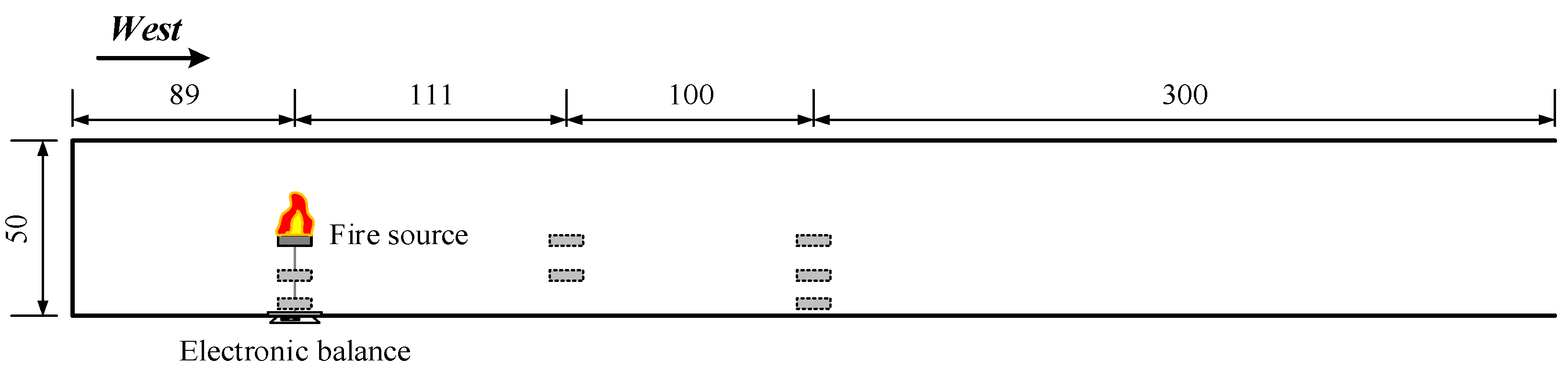
Investigation into the enhanced fuel burning rate was performed in a one-closed-end model tunnel (Figure 7). Its dimensions were 6 m (length) × 0.4 m (width) × 0.5 m (height). Eight tests were conducted. Each test was repeated to ensure the accuracy and repeatability. The fuel pan size was 10 cm × 10 cm × 3 cm and was changed to three vertical and three longitudinal locations. The pan was placed in the middle of the tunnel transversely. Heptane was employed as the fuel. For comparison, a burning test using the same fuel pan was also conducted in open space. The mass of fuel was recorded by an electronic balance (Sartorius Cubis MSE14202S-OCE-DO) with an uncertainty of 0.01 g. Details of each model test can also be found in Table 1.

3. Results and Discussion

3.1. Fire Behaviour of Accommodated Cables

3.1.1. Burning Characteristics and Phenomena

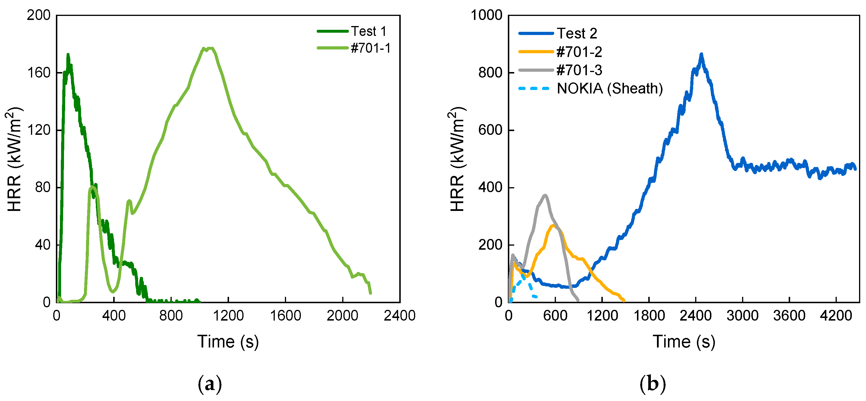
Test 1 and Test 2 were carried out under the radiative heat flux of 24.9 kW/m² and 28.3 kW/m², respectively. In accordance with the recorded video, the burning duration (which started from the ignition to the extinguishment) for each test was 974 s and 4390 s, respectively. The duration of cables burning in Test 2 was thus more than four times longer. As shown in Figure 8, the peak HRR in Test 2 also appeared five times as high as that in Test 1, which is very hazardous. The main peak appeared early in Test 1 but quite late in Test 2. It should be noted that the secondary peak in Test 2 also had a value (165.2 kW/m²) close to the peak in Test 1. This peak emerged slightly earlier (56 s) than that of Test 1 (80 s), which was a result of higher heat flux. Considering the similar shape of curves in the beginning, Test 1 may represent the initial stage of Test 2. Furthermore, the cone calorimeter test results of two other kinds of cables made of similar materials, have been compared. They are the NOKIA AHXCMK 10 kV 3 × 95/70 mm² [12,13] and the 7/C #12AWG 600V [10]. The detailed materials of their components are summarized in

Table 2. Components of the three types of cables.

Test No.	Cable Markings	Diameter (mm)	Sheath	Filler	Insulation	Conductor	Radiative Heat Flux (kW/m2)	Peak Heat Release Rate HRR (kW/m2)
Test 1	ZRC-YJV-8.7/10 3 × 95 mm2	60	PVC	PE	XLPE	Copper	24.9	172.6
Test 2	ZRC-YJV-8.7/10 3 × 95 mm2	60	PVC	PE	XLPE	Copper	28.3	865.6
NOKIA	NOKIA AHXCMK 10 kV 3 × 95/70 mm2	54	PVC	PE	XLPE	Cooper & Aluminium	50	94.5 1
#701-1	7/C #12AWG 600V	14	PVC	-	PE	Copper	25	177.1
#701-2	7/C #12AWG 600V	14	PVC	-	PE	Copper	50	269.3
#701-3	7/C #12AWG 600V	14	PVC	-	PE	Copper	75	373.4

¹ The peak HRR of NOKIA AHXCMK 10 kV 3 × 95/70 mm² is only the peak HRR value of its sheath.

. From Figure 8a, under the same heat flux (25 kW/m²), the main peak HRR in Test #701-1 is comparable to that of Test 1. Additionally, the shape which contained a main peak and a secondary peak and its long duration revealed that the burning was relatively thorough. However, when exposed to a higher heat flux (Figure 8b), the main peak HRR of the 7/C #12AWG 600V cable always remained smaller than half of the peak HRR in Test 2. Note that in Test # 701-2 and Test # 701-3, the rediative heat flux was 50 kW/m² and 75 kW/m², which was much higher than that in Test 2. The HRR of the sheath of the NOKIA AHXCMK 10 kV 3 × 95/70 mm² cable also had a substantially lower peak value.

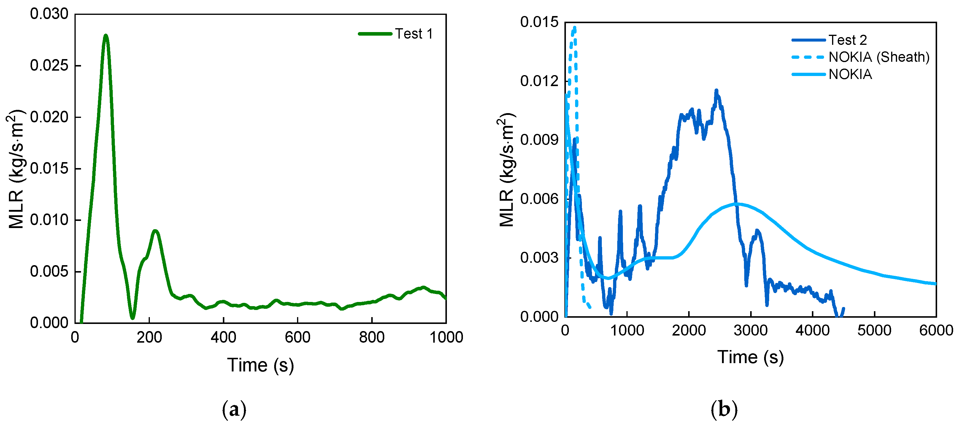
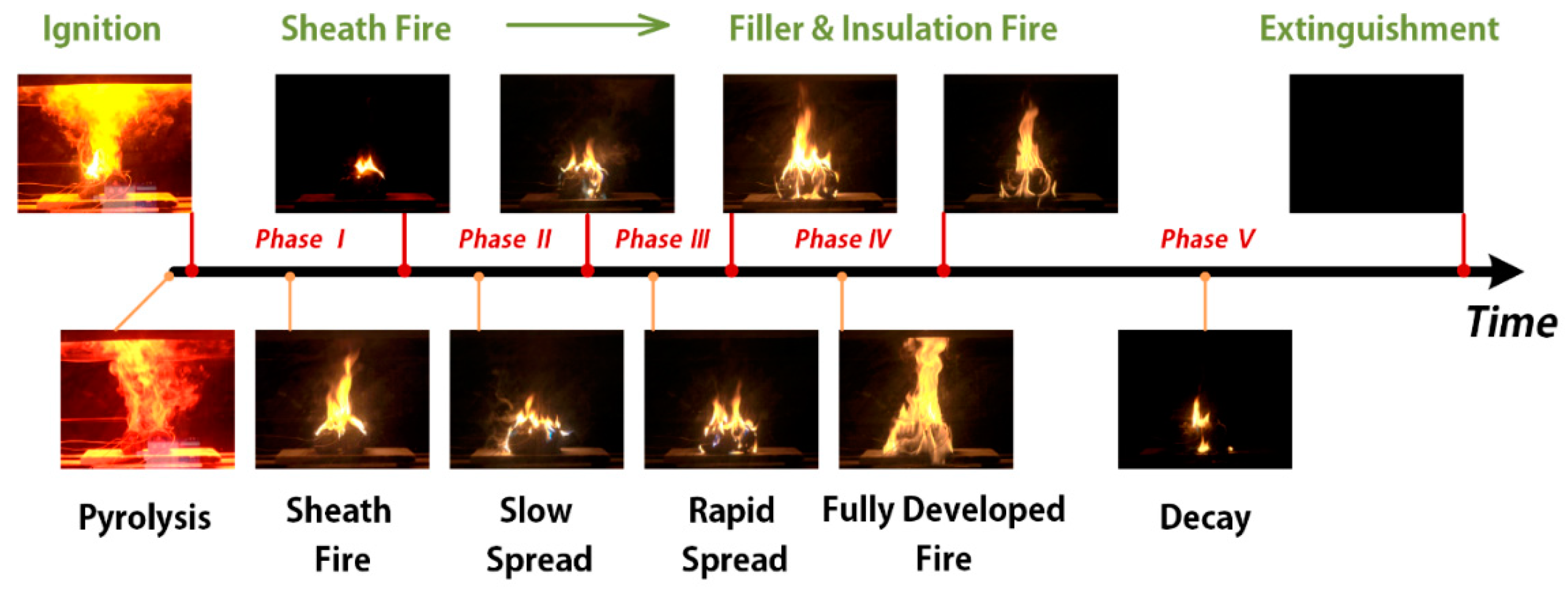
As illustrated in Figure 9, the mass loss rates (MLR) of Cable ZRC-YJV-8.7/10 3 × 95 mm² in Test 1 and Test 2 also show higher peak values than either the sheath of NOKIA AHXCMK 10 kV 3 × 95/70 mm² or the whole cable. In addition, the MLR curve of Test 2 had such a complex trend that needs our further analysis. A careful check of the long-time burning process motivated us to divide it into five phases: the sheath fire, slow spread, rapid spread, full developed fire and decay (Figure 10). Also, in reference to the MLR curve, we decided the points in time between these phases. Detailed descriptions of each phase is listed in

Table 3. Descriptions of different phases during the cable burning process in Test 2.

Phase No.	Phase	Duration	Description
-	Pyrolysis and ignition	12 s (pyrolysis)	The exposed surface of sheath smoked rapidly. After 6 s, the surface was ignited but no sustained ignition was observed. Then, 6 s after, the spark re-ignited the left sample and a part of the flame then jumped onto the right. Two flames merged quickly.
I	Sheath fire	0–744 s	Popping of pieces off the surface occurred on and off. Rapid flashing occurred right under the upper sheath. The samples deformed greatly while burning, with the char surface forming blisters. The burning itself started to decay soon.
II	Slow spread	745–1374 s	The flame on the upper sheath was weak. Flashing under the upper sheath became unobtrusive. The sheath and insulation provided significant thermal protection. In the end, the flame started penetrating the underlying material and blue flames were noted.
III	Rapid spread	1375–1870 s	Filler was on fire, with a large amount of dripping and burning out the bottom. The flame spread fairly deep and the whole surface was touched. Blue flames were inside.
V	Fully developed fire	1871–2600 s	Blue flames became unnoticeable. The whole cable was burning steadily and vigorously. Occasional melted liquid was noticed and the burning area at the bottom became larger.
VI	Decay	2601–4390 s	The fire decayed gradually. Then, flames appeared only on the upper surface and bottom for a while and extinguished finally.

. The burning evolved fairly gradually, from sheath to the filler and insulation inside. The sheath was easy to ignite. It burned quickly to its maximum rate and then declined continuously. Then the fire slowly spread to the underlying PE filler. The traditional characteristics of thermoplastics, such as melting and dripping occurred, resulting in a rapid spread progress. Following from this, the cables burned violently and the HRR reached its maximum. Eventually, all fuels were consumed. Note that the sheath and insulation did provide significant thermal protection in the second phase, but this protection could not always be successful, which was the difference between Test 1 and Test 2. In addition, the PE filler was quite hazardous, as the dripping and burning promoted combustion, increased the burning area and led to a fully developed stage.

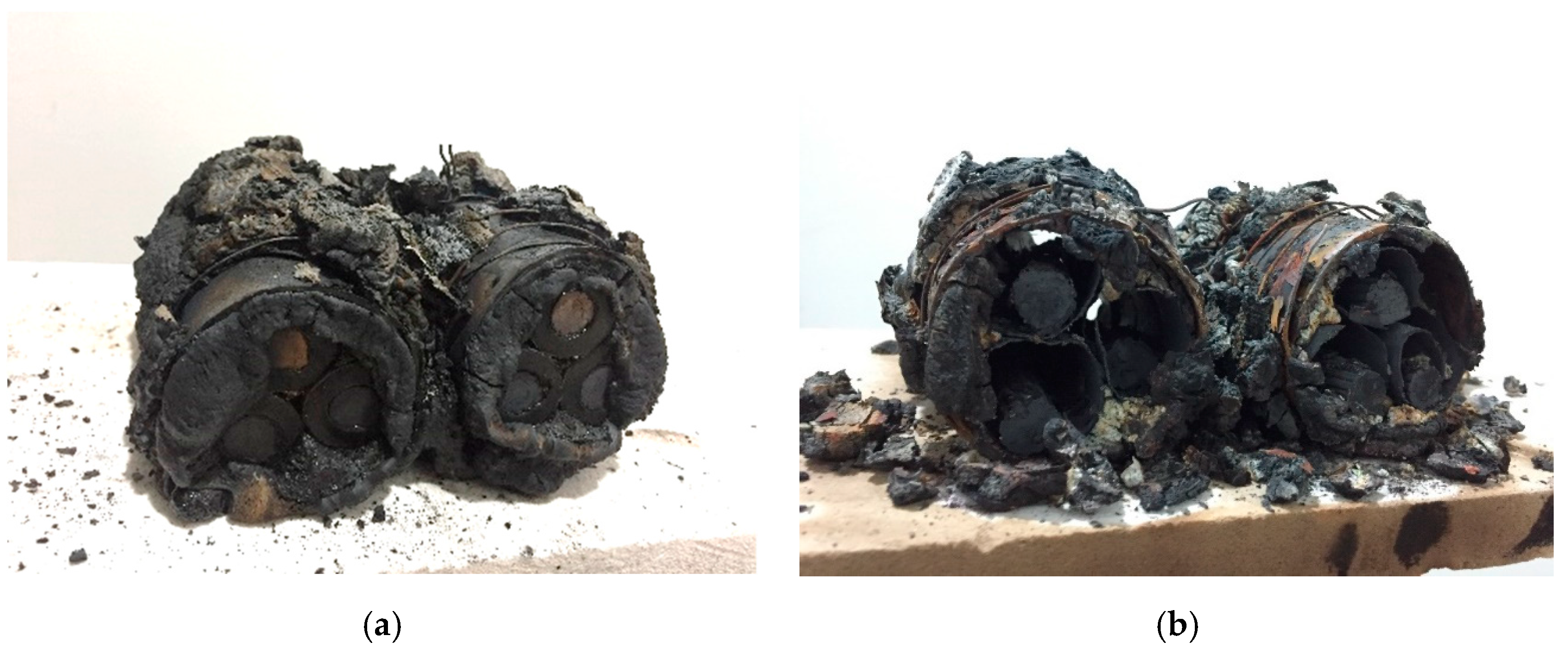
Figure 11 shows the samples of Cable ZRC-YJV-8.7/10 3 × 95 mm² after Test 1 and Test 2. It is obvious that Test 1 was an incomplete combustion case, in accordance with what was discussed. The XLPE insulation nearly did not burn, while only the PVC sheath and a small part of the PE filler were consumed. The cable samples in Test 2 consumed nearly all the fuels. The cables become hollow after the long-time burning, where the PVC sheath, PE filler and XLPE insulation all burned away. The filler swelled notably after Test 1, whereas more residues were spread on the slab after Test 2.

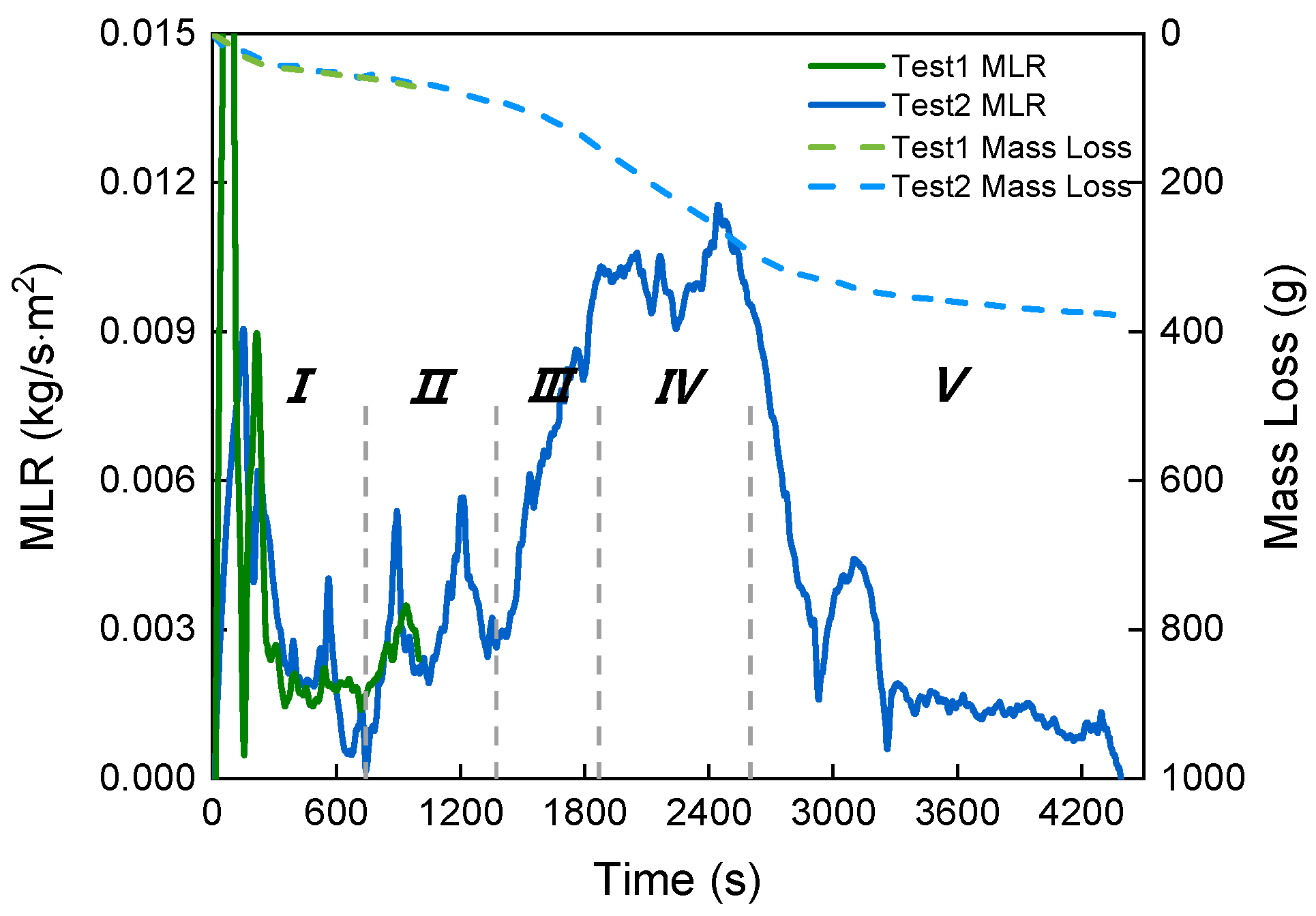
A direct comparison between Test 1 and Test 2 is made in Figure 12. One noteworthy point is that both MLR and mass loss curves of the two tests roughly overlap with each other. We thus confirm that Test 1 can be regarded as the initial stage of the complete burning process (Test 2). Designers should pay attention to the values of parameters in the fourth phase when performing targeted fire safety design.

3.1.2. Combustion Gas Concentration and Cable Surface Temperature

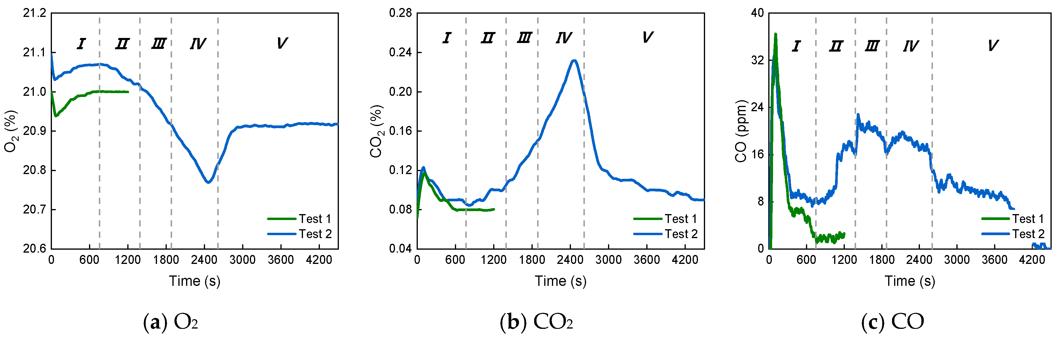
Figure 13 shows the concentrations of O₂, CO₂ and CO. Again, the curves for Test 1 and Test 2 at the initial stage are alike. The O₂ curves are quite analogous to the HRR curves in terms of shape, as the oxygen consumption principle was adopted. The shapes of CO₂ curves are also comparable to HRR curves. The CO concentration in Test 2, on the other hand, had a higher value in the sheath fire stage despite the fact that the combustion was actually more vigorous in the fourth phase. Therefore, combustion at the beginning was relatively incomplete. Much more toxic CO gases mean a danger for workers in the utility tunnel when a fire occurs.

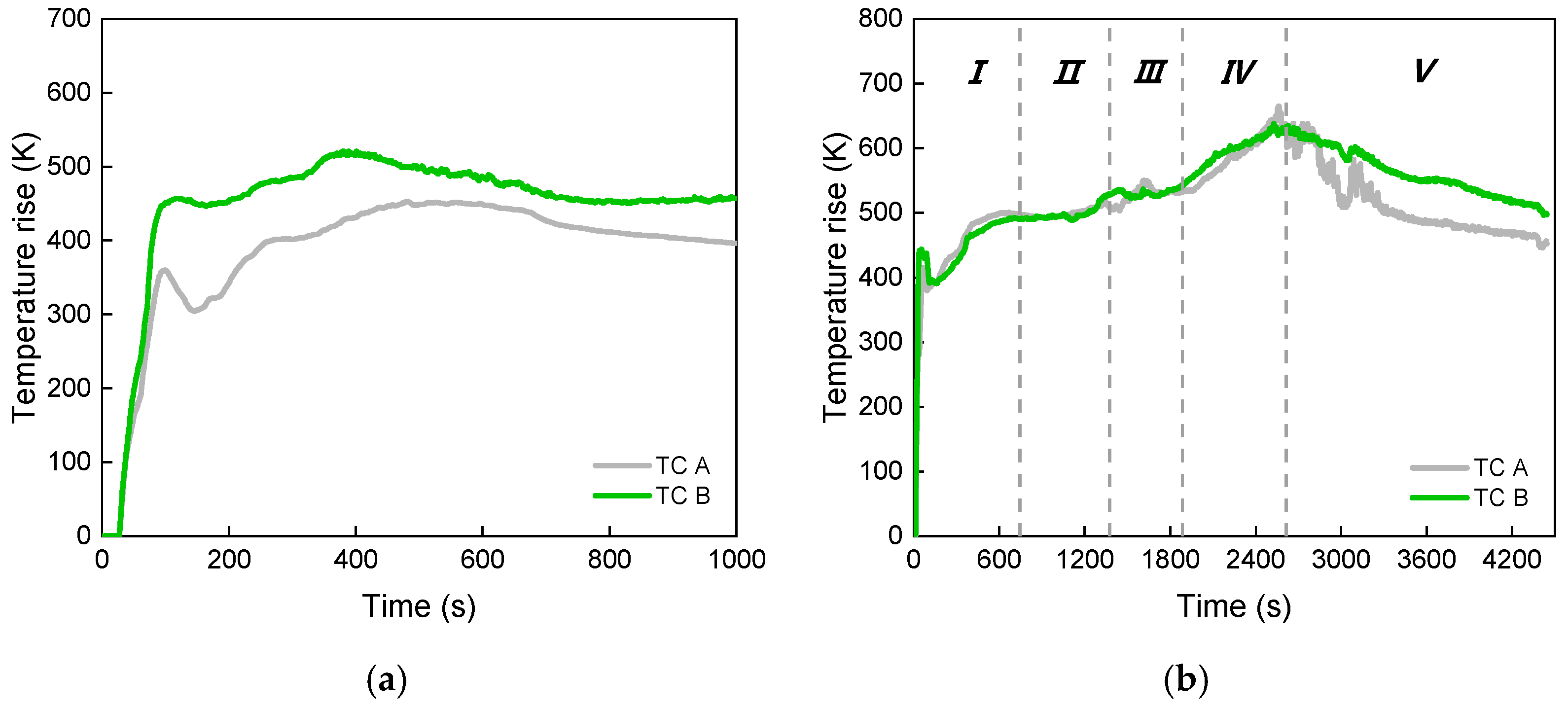
Measured temperatures at two locations are shown in Figure 14. These curves roughly exhibit a similar trend, indicating that the flame was symmetrical for most of the time. The temperature curves also present peaks noticeably early. However, after a short reduction, the temperature values will increase progressively until the summit.

3.2. Temperature Field within the Hot Gas Layer

3.2.1. Two-Dimensional Temperature Field

A total of nine full-scale tests were carried out in a utility tunnel under construction. Only Test S01 is the fully-closed case. In other one-dead-end tests, the fire source was changed to two horizontal locations and three vertical locations for comparison. Firstly, we will observe the size of pool fires we set. The HRR of a pool fire can be estimated as [23]:

$$\dot{Q}=\Delta h_c{\dot{m}}_{\infty }^{″}\left(1-e^{-k\beta D}\right)\times A$$

(1)

where $\dot{Q}$ is the heat release rate (MW), $\Delta h_c$ is the net heat of combustion (MJ/kg), ${\dot{m}}_{\infty }^{″}$ represents the asymptotic mass loss rate per unit area (kg/s·m²) as the pool diameter $D$ (m) increases towards infinity and $A$ represents the fuel burning area (m²). The empirical term is the product of the extinction absorption coefficient $k$ and the beam-length corrector $\beta$. Assuming that the combustion was complete and taking related values into account, the HRR of the two heptane pool fires (40 cm × 40 cm × 20 cm and 60 cm × 60 cm × 20 cm) are calculated as 0.851 MW and 0.282 MW, respectively. In reference to cable Test 2 and considering that normally five parallel cables are placed on a tray in China, these two pool fires then correspond to a burning area of about 2 m or 0.7 m long on a tray.

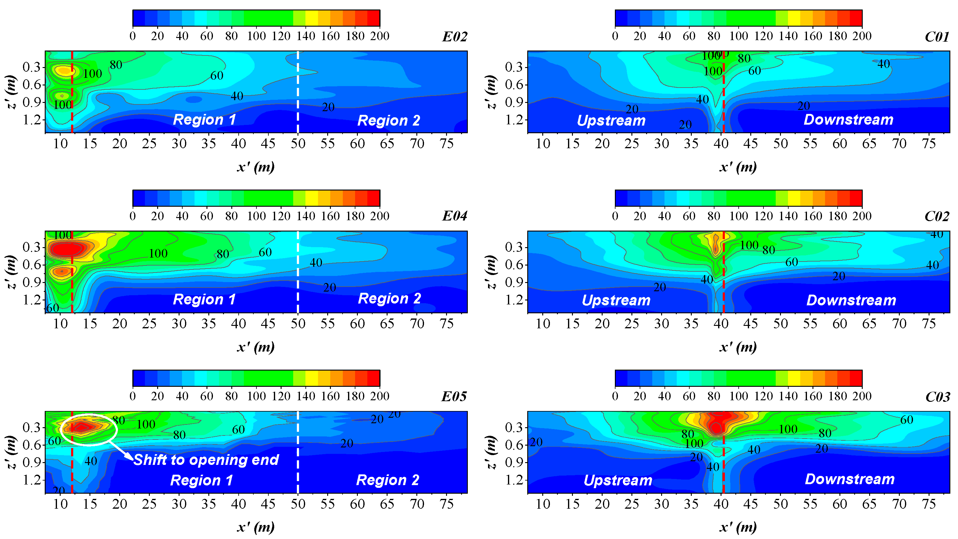
Furthermore, the temperature at each point under steady state was obtained with Ji et al.’s method employed [24]. We then applied 2D interpolation in the data and depicted the temperature field in Figure 15. The red dash lines indicate the fire location, while the white dash lines help us compare the two groups of tests: Test E02, 04, 05 and Test C01, 02, 03. In each diagram, the region above fire is the hottest in the field, and the temperature gradually decreases far away. Areas within the hot gas layer show a “bulge” shape, which should be a characteristic of the hot flow. Evidently, the ceiling clearance H (distance between ceiling and fuel pan) has a great impact on the temperature field. When comparing Test E02, 04 and 05, we can see that as the fire was placed at a higher location, the hot gas layer became thinner. This was because less air would be entrained into the hot gas flow when the flow impinged on the ceiling and propagated away earlier. In opposition to this, the areas between the isothermals with the same values were broader if we compare Test C02 with C01 (or C04 with C02). This is also reasonable, since less air entrainment means less heat loss during the process.

Aside from this, the closed end also played a considerable role. The closed end interrupted the symmetry in the field. As can be seen in Tests C01–03, the upstream gas layer was thicker, and areas between isothermals with the same values were thicker. Moreover, the horizontal distance between the fire source and end wall affected the temperature field as well. Region 1 in the left figures of Figure 15 are compared with the downstream field in the right. The comparisons of Test E02 with C01 and Test E04 with C02 demonstrate that the total downstream smoke layer will be thicker when the fire is set near the end wall. It is also distinct that the areas between the isothermals with the same values also became broader. The possible cause behind the situations is that the upstream gas flowed onto the end and accumulated and then reflected back towards the fire source. The back flow finally pushed the downstream flow out to the portal at the other side and, consequently, the downstream areas became broader. In Test E05, the interaction was very violent and the core high-temperature area shifted to the opening.

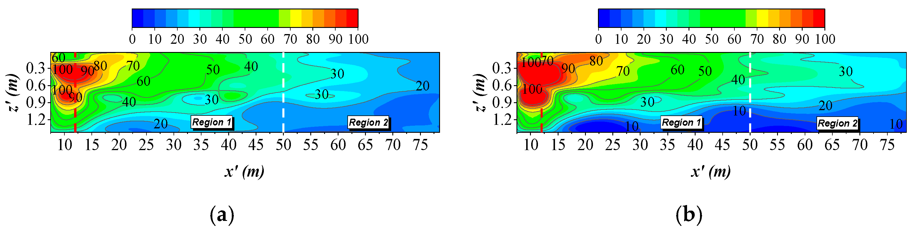
In the fully-closed case, the induced flow pattern was another situation where both upstream flow and downstream flow were restricted and thus backflow was formed at both ends. The difference between Test S01 and E02 was that the downstream end was closed. As depicted in Figure 16, temperature fields were quite similar—in both cases the downstream flow was forced to flow to the west end, due to the accumulated upstream hot gas. The difference was that areas between those isothermals with the same values travelled longer in Test E02. The downstream flow seemed to “encounter resistance” across the whole field. On the other side, the flow was much thicker and almost filled in the space.

3.2.2. Longitudinal Maximum Gas Temperature Decay

As noted, areas within the hot gas layer showed a “bulge” shape. In fact, the convex-concave shape of vertical distributions has already been observed [25]: the temperature increases promptly from the ceiling no-slip condition to the maximum value (the apex) and then decreases gradually away. The self-similarity of the flow has further been confirmed by a function [25,26,27]:

$$\frac{\Delta T_z}{\Delta T_m}=\phi \left(\frac{z}{h_T}\right)$$

(2)

Here, $\Delta T_z$, $\Delta T_m$, $z$ and $h_T$ are the temperature rise at z from the ceiling, maximum temperature rise vertically, distance from the ceiling and ceiling jet thickness, respectively. The current work is centred on the maximum gas temperature distribution along the longitudinal axis.

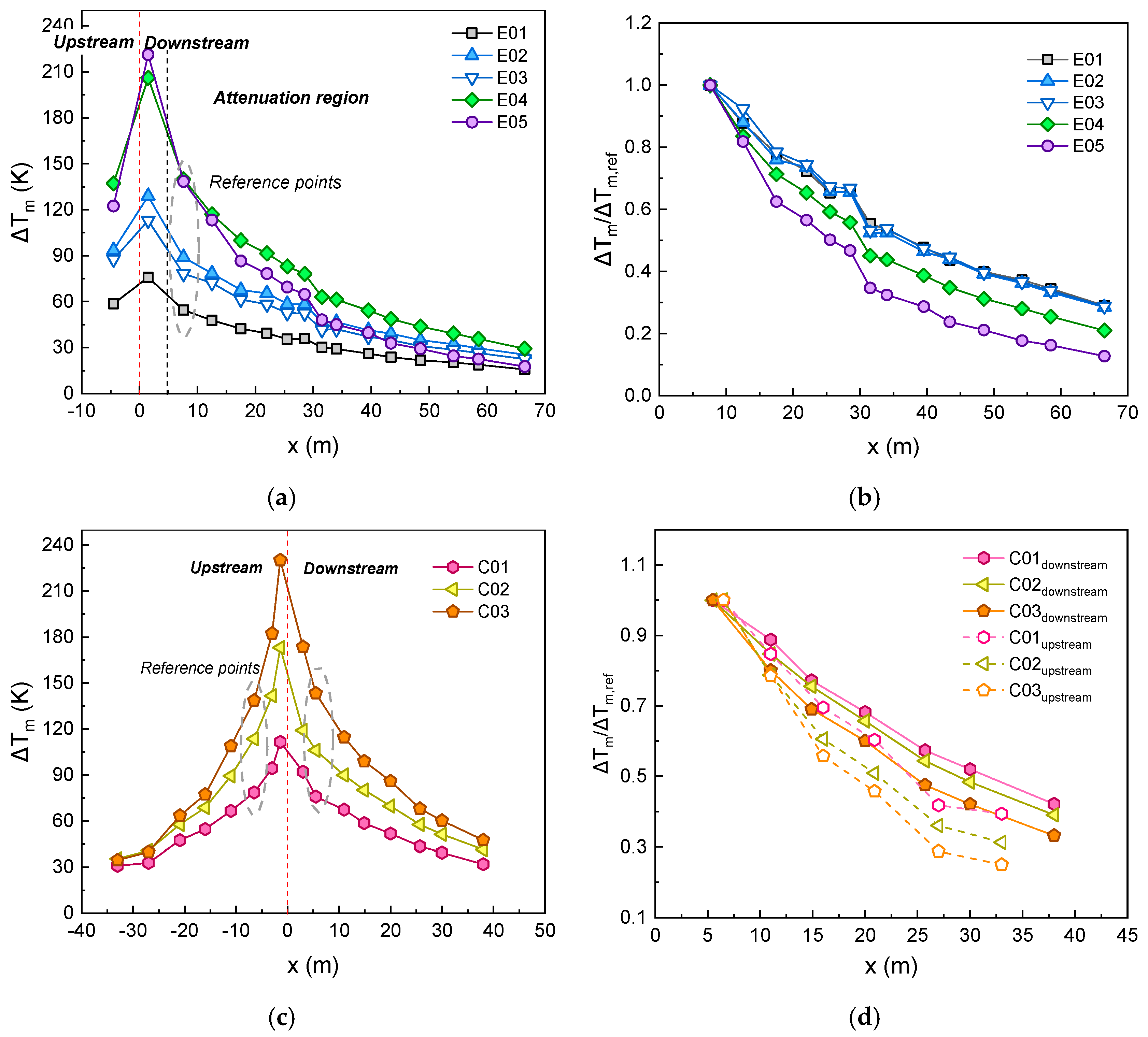
It is clear from Figure 17a that the temperature distributions were affected by the fire size and ceiling clearance H. The fuel burning area in Test E01 was smaller, so the curve appears at the bottom. In other four tests, when the H was reduced from 2.9 m (E02) to 2.4 m (E04), the temperatures generally increased. However, when H continued to decrease to 1.9 m (E05), the temperatures seemed to decay faster in the far field, even approaching those of Test E01. Comparing the results of Test E02 and E03, we can find the test repeatability to be confirmed. Additionally, all the downstream curves show a rapid decay rate near fire and a slower rate far away, which seems to be an exponent-like decay trend. Note that our current focus is on the attenuation region of the complete field, as termed by Gao et al. [28]. The critical beginning position was 1.7 times the plume radius at ceiling level. We approximated the plume radius by tunnel width to obtain a conservative estimation. Therefore, the second position downstream becomes the first measured point of the targeted region and the reference point as well. Dimensionless temperature attenuations are then depicted in Figure 17b. The curves of Test E01–03 overlap quite well, which implies that fire size has very limited influence on the decay rate. When the ceiling clearance decreases, the temperature decay speed increases markedly.

The other group of tests were conducted when fire sources were horizontally placed in the middle. Both the downstream and upstream distributions show an exponent decay shape (Figure 17c). In a similar way, the second point downstream and the third upstream are set as reference points. As shown in Figure 17d, the H had an analogous effect on temperature decay rate. The difference is that the upstream flow temperature attenuated more quickly.

In the following section, we perform a simple derivation in order to obtain the maximum temperature distribution in the hot gas flow in a quasi-steady state. Above all, the vertical difference within the flow will be ignored for simplification.

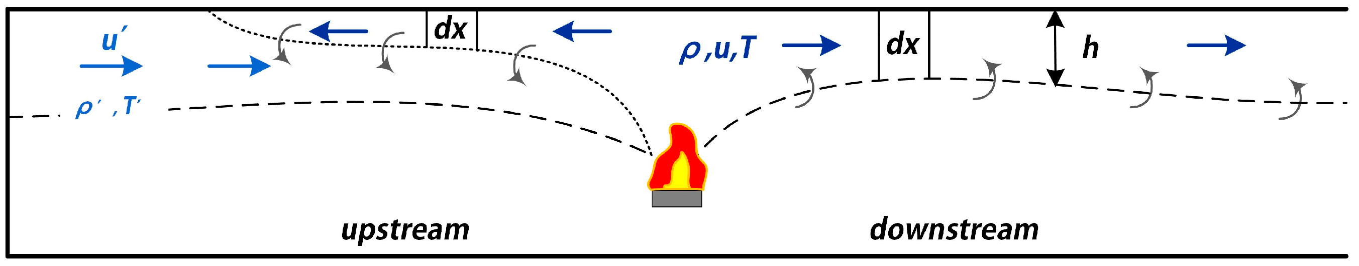
A schematic view of the whole flow is illustrated in Figure 18. The downstream flow entrains fresh air below. Assuming that the temperature of the contact wall surface is the same as the ambient temperature, the mass and energy equations are similar to the longitudinally-ventilated case [4]:

$$\frac{d}{dx}\left(\rho uA\right)={\rho }_{\infty }W{v}_e$$

(3)

$$\frac{d}{dx}\left(\rho uA{c}_{p}T\right)={\rho }_{\infty }W{v}_e{c}_p{T}_{\infty }-h_t{w}_p\left(T-T_{\infty }\right)$$

(4)

In the equations above, the parameters $u$, $v_e$, $A$, $W$, $h_t$, $w_p$, $\rho$ and $T$ are the smoke velocity (m/s), entrainment velocity (m/s), the cross-sectional area of the smoke flow (m²), the tunnel width (m), the total net heat transfer coefficient on tunnel walls (kW/m²·K), the wet perimeter of the smoke flow (m), the average density (kg/m³) and temperature of the smoke flow (K), respectively. The ${\rho }_{\infty }$ and $T_{\infty }$ are ambient density and temperature. We further calculate

$$\frac{\Delta T}{\Delta T_f}=\frac{T-T_{\infty }}{T_f-T_{\infty }}=exp\left(-a\frac{x}{h}\right)$$

(5)

where

$$a=\frac{h_t\left(1+2h/W\right)+{\rho }_{\infty }{v}_e{c}_p}{\rho u{c}_p}$$

(6)

where $x$ is the distance from the fire source (m), $h$ is the smoke layer height (m) and $\Delta T_f$ is the average gas temperature rise above fire (K). The solution above is obtained if we presume that the term $h/W$ varies in a narrow range and $a$ is then considered as a constant. In this case, the gas temperature becomes a single exponent function of distance $x$.

The behaviour of upstream flow is different. We assume that the backflow could entrain the incoming upstream flow when it flows underneath. The mass and energy equations are then presented as

$$\frac{d}{dx}\left(\rho uA\right)=-\rho W{v}_e{}^{\prime }$$

(7)

$$\frac{d}{dx}\left(\rho uA{c}_{p}T\right)=-\rho W{v}_e{}^{\prime }{c}_{p}T-h_t{w}_p\left(T-T_{\infty }\right)$$

(8)

Taking the similar assumption, the final solution can be integrated as

$$\frac{\Delta T}{\Delta T_f}=exp\left(-b\frac{x}{h}\right)$$

(9)

where

$$b=\frac{h_t\left(1+2h/W\right)}{\rho u{c}_p}$$

(10)

It should be noted that the flow itself has been demonstrated to be self-similar. Therefore, the ratio of ceiling jet thickness to smoke flow thickness $h_T/h$, which represents the relative position of two specific proportions of $\Delta T_m$, should be a constant throughout the flow field. We then use the characteristic thickness $h_T$ instead. Finally, if Ingason and Li’s hypothesis could also be employed here, and the maximum temperature distribution $\Delta T_m$ can be correlated through Equations (5) and (9) [17], the equations can be rewritten to predict the temperature decay from a reference point $x_{ref}$ for downstream flow:

$$\frac{\Delta T_m}{\Delta T_{m,ref}}=exp\left[-K_d\left(\frac{x}{h_T}-\frac{x_{ref}}{h_{T,ref}}\right)\right]$$

(11)

For upstream flow:

$$\frac{\Delta T_m}{\Delta T_{m,ref}}=exp\left[-K_u\left(\frac{x}{h_T}-\frac{x_{ref}}{h_{T,ref}}\right)\right]$$

(12)

Here, the attenuation coefficients $K_d$ and $K_u$ directly correlate to the parameters $a$ and $b$, respectively. $\Delta T_{m,ref}$ is the maximum temperature rise at $x_{ref}$. Equations (11) and (12) are adopted to estimate the one-dimensional longitudinal maximum gas temperature decay. The two attenuation coefficients will be determined from the experiment results.

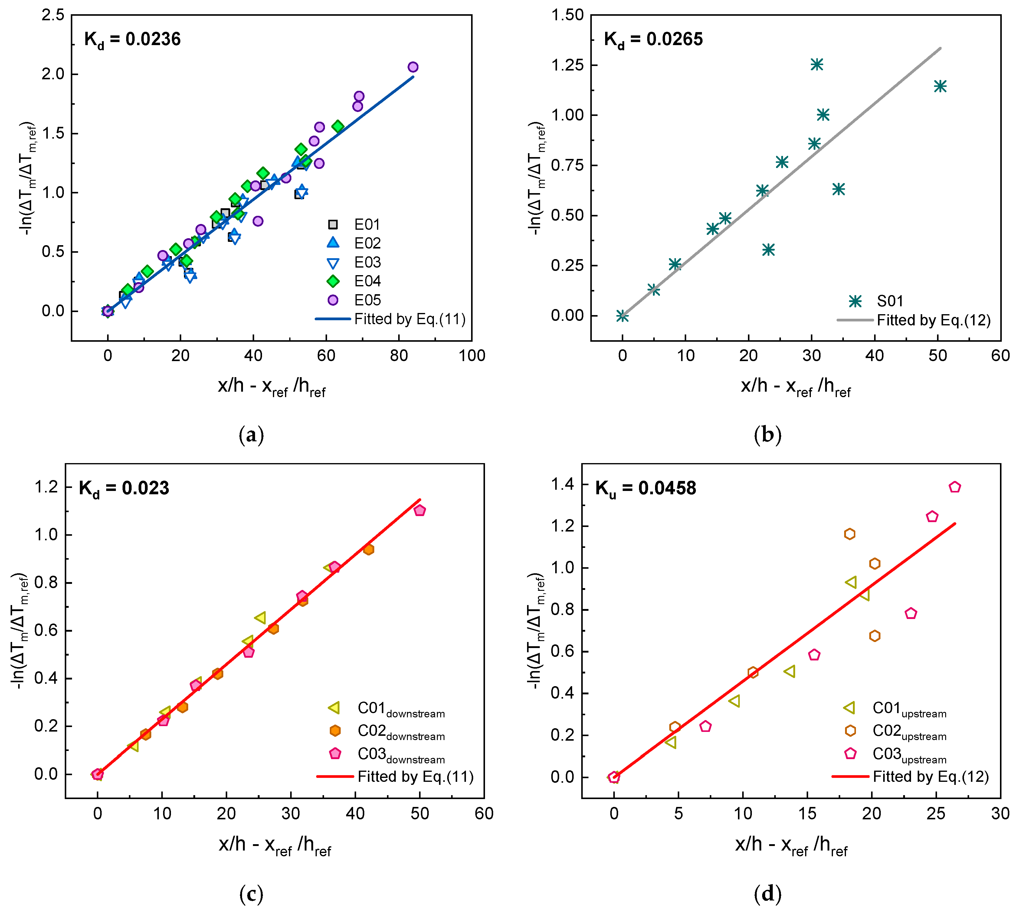
All the fitting results could be seen in Figure 19. Related coefficients and the variances of fitting are listed in

Table 4. Fitting results of all full-scale tests.

Test No.	${\mathit{K}}_{\mathit{d}}$	${\mathit{R}}^2 \mathit{o}\mathit{f} {\mathit{K}}_{\mathit{d}}$	${\mathit{K}}_{\mathit{u}}$	${\mathit{R}}^2 \mathit{o}\mathit{f} {\mathit{K}}_{\mathit{u}}$
E01–05	0.0236	0.985	-	-
C01–03	0.0230	0.998	0.0458	0.964
S01	0.0265	0.935	-	-

. These fitting results are reasonably good, with their coefficients of determination (R-Square) being greater than 0.9. Regardless of fire size or ceiling clearance, the test data coincide with the same line. Indeed, the form of Equations (11) and (12) should be effective. As the fuel pan moved to a higher position, the temperatures decayed faster. On the other side, the H had an opposite effect on the thickness of the flow. When it decreased, the flow became thinner. In each of Tests C01–03, the upstream flow was much thicker than the downstream flow. Our analytical solutions actually consider these two effects in a function concurrently, yielding a single decay coefficient. But a litter divergence was still observed in the far field upstream in Test C01–03 and downstream in Test S01, where the closed end wall was nearby, with this being inevitable. The flow near the end wall was considerably drastic and out of order, and the backflow had a much more complex influence on the incoming flow rather than steadily entraining it as we assumed. We may also find that the coefficients $K_d$ in Test E01–05 and C01–03 are very close, so that the downstream attenuation coefficient $K_d$ could be set as 0.023, regardless of the horizontal fire location. By contrast, the $K_u$ was much larger and it seemed to decrease as the fire source moved away from the end wall.

3.3. Enhanced Fuel Burning Rates in a Utility Tunnel

The fuel burning in a tunnel has been proven to be much more hazardous when compared with the same fuel burning in the open in terms of the burning rate/heat release rate. It has been confirmed that the geometry—the width $W_T$ and height $H_T$ of the tunnel—both influence the burning. However, which one has a dominant effect is still disputable. To date, the impact of the tunnel end wall on the burning has not been investigated either.

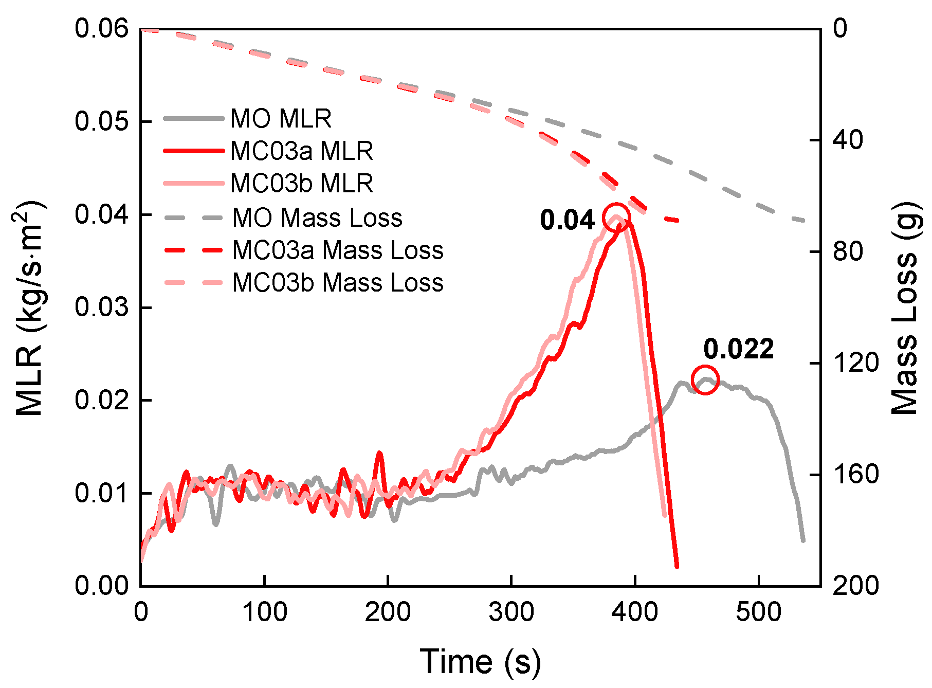
Figure 20 shows the MLR and mass loss of the heptane fuel in Test MO and Test MC03. Note that the repeatability of tests is validated, which was proven by the two results of Test MC03. When compared with the result of Test MO, the burning rate in Test MC03 was enhanced substantially after about 200 s. The peak MLR had a value of 0.04 kg/s·m², which is 1.8 times the peak value of the free burn test. The burning duration is reduced as a result.

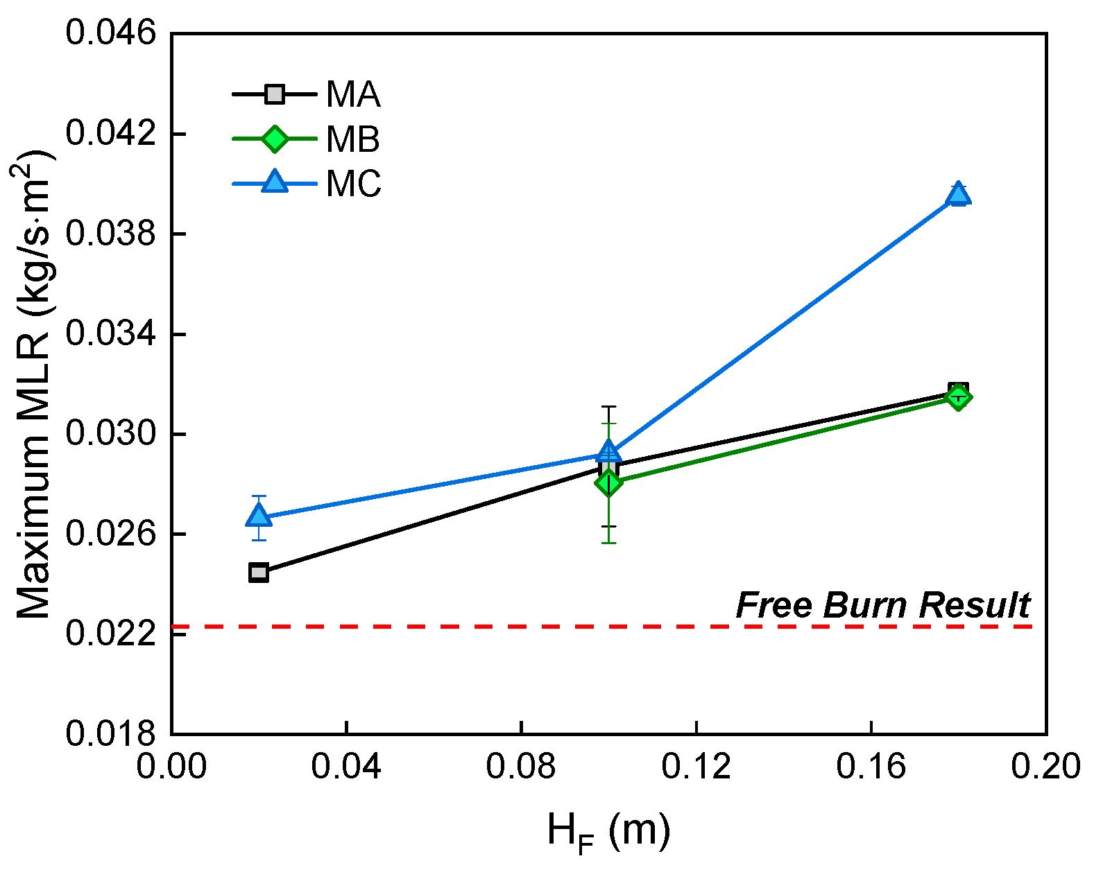
Results of the maximum MLR in the remaining tests can be seen in Figure 21. The enhancement appears in all tests. As the vertical distance between fuel and tunnel floor $H_F$ increased, the peak MLR increased following a more exponent-like tendency. However, the increasing trend seems to depend on the horizontal position of fuel also. When the pool fire was set close to the end wall, the enhanced MLR decreased to a certain value. The decrease was fairly rapid at the beginning but became inconspicuous further on. This reveals that the relationship between the distance $L_F$ (fire source to end wall) and enhanced MLR might also be an exponential function.

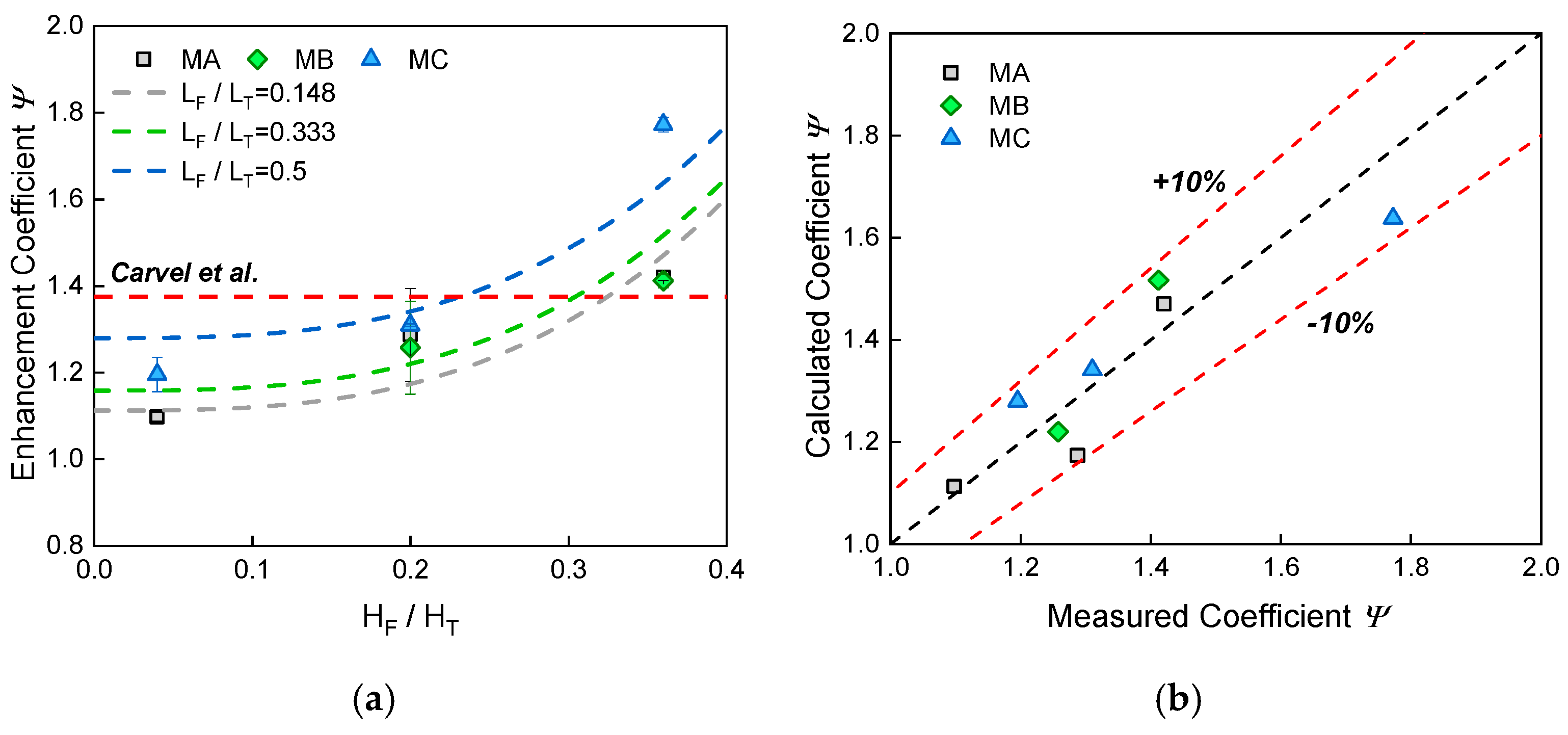
Apart from the factors $H_F$ and $L_F$, the fuel pan width $W_F$ is believed to be an important term as well. Though the ratio $\frac{W_F}{W_T}$ has not been changed in current study, Carvel et al. [18] identified it to be the most influential factor on the basis of abundant test results. Also, in a similar manner to Carvel et al., we aimed our attention at the MLR enhancement coefficient $\Psi$, denoted by the MLR of a fire in a tunnel divided by the MLR of a similar fire in open space. Carvel et al. concluded that $\Psi$ varies as a single cubic function of $\frac{W_F}{W_T}$, while we simply modified it based on our analysis:

$$\Psi =\alpha {\left(\frac{W_F}{W_T}\right)}^3+\beta {\left(\frac{H_F}{H_T}\right)}^3+\gamma {\left(\frac{L_F}{L_T}\right)}^3+1$$

(13)

where $\alpha , \beta , \gamma$ are empirical coefficients which are determined by the experimental results. The values of these parameters actually indicate the roles of the relative scales $\frac{W_F}{W_T}$, $\frac{H_F}{H_T}$ and $\frac{L_F}{L_T}$ on the enhancement. The final fitting result of the multivariate nonlinear regression of all the test data is then written as

$$\Psi =6.91{\left(\frac{W_F}{W_T}\right)}^3+7.67{\left(\frac{H_F}{H_T}\right)}^3+1.37{\left(\frac{L_F}{L_T}\right)}^3+1$$

(14)

The coefficient of determination (R-Square) is 0.811. From the coefficients of Equation (14), we could see the relative height has an effect on the enhancement that is comparable to the impact of relative width. The influence of relative distance is much smaller. The change caused by $\frac{L_F}{L_T}$ is also moderate due to the fact that the length of tunnel is normally much larger than its width or height. Figure 22a shows the estimated enhancement coefficients under different $\frac{L_F}{L_T}$. The estimated curves generally fit with measured data points. Equation (14) predicts all test results with a relative error smaller than 10%, as could be seen in Figure 22b. In the tests reported in Carvel et al.’s work, fires are often set on the ground. Note that in our similar case, when $\frac{H_F}{H_T}$ is near zero, $\Psi$ is always smaller than that predicted by Carvel et al.’s correlation. This may be caused by the restricted ventilation for combustion, a result that the closed end brings.

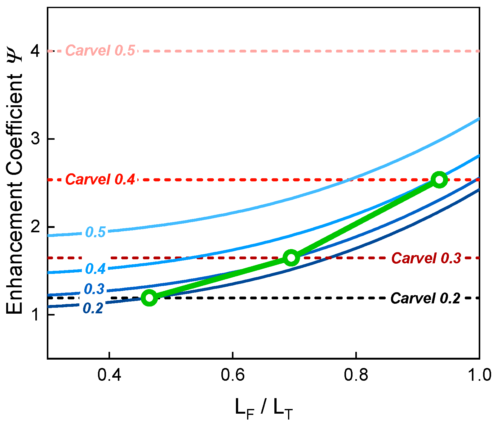
We further suppose that appropriate ranges of $\frac{L_F}{L_T}$ exist, and they should be identified for the applicability of Equation (14). Beyond this range, that is, when the fire is set close to the open portal, the dead end should no longer have an effect on the enhanced MLR. The condition is then similar to a common tunnel with both ends open, which was the focus of Carvel et al.’s work. However, we examined those cases where the fire is set on the ground only for comparison with Carvel’s finding, and thus the second term in Equation (14) equals zero. As shown in Figure 23, when $\frac{W_F}{W_T}=0.2$, the curves predicted by Equation (14) and Carvel’s intersects at $\frac{L_F}{L_T}=0.46$. When $\frac{W_F}{W_T}$ becomes larger, e.g., 0.3 and 0.4, the curves then intersect at $\frac{L_F}{L_T}=0.7$ and $\frac{L_F}{L_T}=0.93$, respectively. Thus, this range is believed to be broader when the fuel pan width gets larger.

However, Equation (14) has its limitations at extreme conditions. When the fuel pan moves to an extremely high position, i.e., $\frac{H_F}{H_T}$ approaches 1, or the fuel pan has a size as large as the tunnel width, i.e., $\frac{W_F}{W_T}$ approaches 1, an incredibly huge $\Psi$ is generated using the Equation (14). In fact, the highly under-ventilated situation should occur in these cases, where similar phenomena have already been observed in the Ofenegg tunnel tests [29] and quite small $\Psi$ of these tests calculated by Ingason [30]. In addition, when the fuel pan moves very deep inside, the under-ventilated situation may also occur, probably yielding a $\Psi$ smaller than 1. This is also not considered in our model. Addressing these problems still remains as a future task where more test data are needed.

4. Conclusions

A comprehensive analysis of the potential fire problems in an urban utility tunnel has been performed, based on a series of bench-scale tests, full-scale tests and model-scale tests. The burning behaviour of accommodated cables, temperature field of hot gas layer and enhanced fuel burning rates were quantitatively explored. The following conclusions were obtained:

(1)

The critical exposed radiative heat flux for the ZRC-YJV-8.7/10 3 × 95 mm² power cable to achieve complete combustion lies in the range from 24.9 kW/m² to 28.3 kW/m². Compared with incomplete burning, its burning duration was more than four times longer and the peak HRR was five times as high (865.6 kW/m²). The incomplete burning was similar to the initial stage of the complete burning. Compared with other cables, i.e., NOKIA AHXCMK 10 kV 3 × 95/70 mm² and 7/C #12AWG 600V, the ZRC-YJV-8.7/10 3 × 95 mm² cable has a generally similar HRR/MLR evolving trend but with significantly greater hazard, even under a lower heat flux.

(2)

The whole burning process was gradual from the outside to the inside and can be divided into five phases: the sheath fire, slow spread, rapid spread, full developed fire and decay. The dripping and burning behaviours of the thermoplastic filler promoted the combustion, increased the burning area and led to a fully developed stage. The PVC sheath and XLPE insulation provided significant thermal protection in the second phase. The toxic CO was rapidly produced in the first phase.

(3)

When the ceiling clearance H increased, the gas layer became thinner and the maximum gas temperature attenuated more quickly. The closed end interrupted the symmetry in the flow field, wherein the upstream flow became thicker and the related temperature decayed faster.

(4)

With the different behaviours of upstream flow and downstream flow considered, an analytical model was developed. The exponent model took fire size and ceiling clearance into account and is able to predict the maximum gas temperature attenuation of both flows reasonably well. The fully-closed case has also been estimated.

(5)

The phenomenon of enhanced fuel burning in a utility tunnel should be carefully treated. This enhancement is affected by $\frac{W_F}{W_T}$, $\frac{H_F}{H_T}$ and $\frac{L_F}{L_T}$ simultaneously. Carvel et al.’s model was modified to integrate the effects of these factors. $\frac{W_F}{W_T}$ and $\frac{H_F}{H_T}$ are further found to have a comparable effect on the enhancement while the influence of $\frac{L_F}{L_T}$ is much smaller. The closed end restricts the ventilation available for combustion but should have no effect as the fuel moves close to the open portal. The current model is thus believed to work within a suitable range of $\frac{L_F}{L_T}$

The study helps to develop a preliminary understanding of fire phenomena in a utility tunnel. The findings can provide designers and operators with valuable guidance for the integrated promotion of a tunnel’s fire safety level.

References

- Cano-Hurtado, J.; Canto-Perello, J. Sustainable development of urban underground space for utilities. Tunn. Undergr. Space Technol. 1999, 14, 335–340. [Google Scholar] [CrossRef]
- Canto-Perello, J.; Curiel-Esparza, J. An analysis of utility tunnel viability in urban areas. Civ. Eng. Environ. Syst. 2006, 23, 11–19. [Google Scholar] [CrossRef]
- Beard, A.; Carvel, R. The Handbook of Tunnel Fire Safety; Thomas Telford Ltd.: London, UK, 2005. [Google Scholar]
- Ingason, H.; Li, Y.Z.; Lönnermark, A. Tunnel Fire Dynamics; Springer: Berlin, Germany, 2014. [Google Scholar]
- Ko, J. Study on the Fire Risk Prediction Assessment due to Deterioration contact of combustible cables in Underground Common Utility Tunnels. J. Korean Soc. Disaster Inf. 2015, 11, 135–147. [Google Scholar] [CrossRef] [Green Version]
- Liang, K.; An, W.; Tang, Y.; Cong, Y. Study on cable fire spread and smoke temperature distribution in T-shaped utility tunnel. Case Stud. Therm. Eng. 2019, 14, 100433. [Google Scholar] [CrossRef]
- Hurley, M.J.; Gottuk, D.T.; Hall, J.R., Jr.; Harada, K.; Kuligowski, E.D.; Puchovsky, M.; Watts, J.M., Jr.; Wieczorek, C.J. SFPE Handbook of Fire Protection Engineering; Springer: Berlin, Germany, 2015. [Google Scholar]
- Grayson, S.J. Fire Performance of Electric Cables-New Test Methods and Measurement Techniques; Final report of EU SMT project SMT4- CT96-2059; Interscience Communications Ltd.: London, UK, 2000. [Google Scholar]
- Commission, University of Nevada. Reno Cable Response to Live Fire (CAROLFIRE); NCR: Rockville, MD, USA, 2008; Volume 1–3. [Google Scholar]
- McGrattan, K.B.; Lock, A.J.; Marsh, N.D.; Nyden, M.R. Cable Heat Release, Ignition, and Spread in Tray Installations During Fire (CHRISTIFIRE): Phase 1-Horizontal Trays; National Institute of Standards and Technology: Gaithersburg, MD, USA, 2012.
- McGrattan, K.B.; Bareham, S.D. Cable Heat Release, Ignition, and SPREAD in Tray Installations during Fire (CHRISTIFIRE) Phase 2: Vertical Shafts and Corridors| NIST; NIST: Gaithersburg, MD, USA, 2013.
- Matala, A.; Hostikka, S. Probabilistic simulation of cable performance and water based protection in cable tunnel fires. Nucl. Eng. Des. 2011, 241, 5263–5274. [Google Scholar] [CrossRef]
- Matala, A.; Hostikka, S. Pyrolysis modelling of PVC cable materials. Fire Saf. Sci. 2011, 10, 917–930. [Google Scholar] [CrossRef]
- Delichatsios, M.A. The flow of fire gases under a beamed ceiling. Combust. Flame 1981, 43, 1–10. [Google Scholar] [CrossRef]
- Hu, L.; Huo, R.; Chow, W.K.; Wang, H.; Yang, R. Decay of buoyant smoke layer temperature along the longitudinal direction in tunnel fires. J. Appl. Fire Sci. 2004, 13, 53–77. [Google Scholar] [CrossRef]
- Hu, L.; Huo, R.; Li, Y.; Wang, H.; Chow, W. Full-scale burning tests on studying smoke temperature and velocity along a corridor. Tunn. Undergr. Space Technol. 2005, 20, 223–229. [Google Scholar] [CrossRef]
- Ingason, H.; Li, Y.Z. Model scale tunnel fire tests with longitudinal ventilation. Fire Saf. J. 2010, 45, 371–384. [Google Scholar] [CrossRef]
- Carvel, R.; Beard, A.; Jowitt, P.; Drysdale, D. The influence of tunnel geometry and ventilation on the heat release rate of a fire. Fire Technol. 2004, 40, 5–26. [Google Scholar] [CrossRef]
- Lönnermark, A.; Ingason, H. The Effect of Cross-sectional Area and Air Velocity on the Conditions in a Tunnel during a Fire; SP Technical Research Institute of Sweden: Borås, Sweden, 2007. [Google Scholar]
- Li, Y.Z.; Fan, C.G.; Ingason, H.; Lönnermark, A.; Ji, J. Effect of cross section and ventilation on heat release rates in tunnel fires. Tunn. Undergr. Space Technol. 2016, 51, 414–423. [Google Scholar] [CrossRef]
- Huggett, C. Estimation of rate of heat release by means of oxygen consumption measurements. Fire Mater. 1980, 4, 61–65. [Google Scholar] [CrossRef]
- International Standard Organization. Reaction-to-Fire Tests-Heat Release, Smoke Production and Mass Loss Rate-Part 1: Heat Release Rate (Cone Calorimeter Method); ISO: Geneva, Switzerland, 2002. [Google Scholar]
- Babrauskas, V. Heat release rates. In SFPE Handbook of Fire Protection Engineering; Springer: Berlin, Germany, 2016; pp. 799–904. [Google Scholar]
- Ji, J.; Zhong, W.; Li, K.; Shen, X.; Zhang, Y.; Huo, R. A simplified calculation method on maximum smoke temperature under the ceiling in subway station fires. Tunn. Undergr. Space Technol. 2011, 26, 490–496. [Google Scholar] [CrossRef]
- Oka, Y.; Oka, H.; Imazeki, O. Ceiling-jet thickness and vertical distribution along flat-ceilinged horizontal tunnel with natural ventilation. Tunn. Undergr. Space Technol. 2016, 53, 68–77. [Google Scholar] [CrossRef]
- Davis, W.D.; Cooper, L.Y. Estimating the Environment and the Response of Sprinkler Links in Compartment Fires with Draft Curtains and Fusible-Link-Actuated Ceiling Vents: User Guide for the Computer Code LAVENT; US Department of Commerce, National Institute of Standards and Technology: Gaithersburg, MD, USA, 1989.
- Motevalli, V.; Marks, C.H. Characterizing the unconfined ceiling jet under steady-state conditions: A reassessment. Fire Saf. Sci. 1991, 3, 301–312. [Google Scholar] [CrossRef]
- Gao, Z.; Liu, Z.; Wan, H.; Zhu, J. Experimental study on longitudinal and transverse temperature distribution of sidewall confined ceiling jet plume. Appl. Therm. Eng. 2016, 107, 583–590. [Google Scholar] [CrossRef]
- Haerter, A. Fire tests in the Ofenegg-Tunnel in 1965. In Proceedings of the International Conference on Fires in Tunnels, SP REPORT, London, UK, 15 December 1998; pp. 195–214. [Google Scholar]
- Ingason, H. Fire testing in road and railway tunnels. In Flammability Testing of Materials Used in Construction, Transport and Mining; Elsevier: Amsterdam, The Netherlands, 2006; pp. 231–274. [Google Scholar]
Figure 1.
A common utility tunnel.
Figure 2.
Schematic of the calorimeter apparatus.
Figure 3.
Cross-section of the ZRC-YJV-8.7/10 3 × 95 mm2 power cable.
Figure 4.
Photos of the experiment compartment in a utility tunnel under construction: (a) the full-scale utility tunnel; (b) the compartment cross section.
Figure 5.
Schematic diagram of the full-scale test rig (dimensions in cm).
Figure 6.
Vertical temperature measuring positions of a thermocouple pile (dimensions in cm).
Figure 7.
Schematic diagram of the model-scale test rig (dimensions in cm).
Figure 8.
Heat release rates for Cable ZRC-YJV-8.7/10 3 × 95 mm2 in: (a) Test 1; (b) Test 2 in comparison with other cable tests.
Figure 9.
Mass loss rates for Cable ZRC-YJV-8.7/10 3 × 95 mm2 in: (a) Test 1; (b) Test 2 in comparison with other cable tests.
Figure 10.
Snapshots of different phases during Test 2.
Figure 11.
Photographs of Cable ZRC-YJV-8.7/10 3 × 95 mm2 samples after each test: (a) after Test 1 at 24.9 kW/m2; (b) after Test 2 at 28.3 kW/m2.
Figure 12.
Mass loss rates and mass losses for Cable ZRC-YJV-8.7/10 3 × 95 mm2 in Test 1 and Test 2. MLR—mass loss rates.
Figure 13.
Concentrations of O2, CO2 and CO of combustion gas for Cable ZRC-YJV-8.7/10 3 × 95 mm2 in Test 1 and Test 2.
Figure 14.
Measured temperatures for Cable ZRC-YJV-8.7/10 3 × 95 mm2 in: (a) Test 1; (b) Test 2.
Figure 15.
Temperature distribution of the hot gas layer in one-dead-end cases (Unit: K).
Figure 16.
Temperature distribution of the hot gas layer in: (a) Test S01; (b) Test E02 (Unit: K).
Figure 17.
The longitudinal distribution of maximum gas temperature along the tunnel: (a) temperature distribution in Test E01–05; (b) dimensionless temperature distribution in Test E01–05; (c) temperature distribution in Test C01–03; (d) dimensionless temperature distribution in Test C01–03.
Figure 18.
A diagram of upstream and downstream flow within a ceiling jet.
Figure 19.
Fitting results of the longitudinal maximum gas temperature distribution in: (a) Test E01–05; (b) Test S01; (c) Test C01–03 downstream; (d) Test C01–03 upstream.
Figure 20.
Mass loss rates and mass losses for heptane fuel in Test MO and Test MC03.
Figure 21.
Mass loss rates for heptane fuel in all model-scale tests.
Figure 22.
Comparison between experimental and estimated results of enhancement coefficient: (a) measured data and estimated curves; (b) calculated data and measured data.
Figure 23.
Determination of the appropriate ranges of where the current model works.