Optimized Design of the District Heating System by Considering the Techno-Economic Aspects and Future Weather Projection

Abstract

High mountains and cold climate in the north-west of Iran are critical factors for the design of optimized District Heating (DH) systems and energy-efficient buildings. It is essential to consider the Life Cycle Cost (LCC) that includes all costs, such as initial investment and operating costs, for designing an optimum DH system. Moreover, considering climate change for accurately predicting the required heating load is also necessary. In this research, a general optimization is carried out for the first time with the aim of a new design concept of a DH system according to a LCC, while considering all-involved parameters. This optimized design is based on various parameters such as ceiling and wall insulation thicknesses, depth of buried water and heating supply pipes, pipe insulation thickness, and boiler outlet temperature. In order to consider the future weather projection, the mentioned parameters are compared with and without climate change effects in a thirty-year period. The location selection was based on the potential of the region for such a system together with the harsh condition of the area to transport the common fossil fuel to the residential buildings. The obtained results show that insulation of walls is more thermally efficient than a roof with the same area in the selected case. In this case, polyurethane is the best material, which can cause a reduction of 59% in the heating load and, consequently, 2332 tons of CO₂ emission annually. The most and the least investment payback periods are associated with the polyurethane and the glass wool insulation materials with the amounts of seven and one years. For the general optimization of the DH system, the Particle Swarm Optimization (PSO) method with a constriction coefficient was chosen. The results showed that the optimal thickness of the polyurethane layer for the thermal insulation of the building exterior walls is about 14 cm and the optimal outlet temperature of the boiler is about 95 °C. It can be also concluded that the optimal depth for the buried pipes is between 1.5 to 3 m underground. In addition, for the pipe with elastomeric insulation layer, the thickness of 2 cm is the optimal choice.

1. Introduction

Energy demands and environmental problems at present are the main sources of concern for human life. By increasing the population, the energy demand is reaching its highest level. On the other hand, the environment is threatened, by increasing greenhouse gas (GHG) emissions [1]. Therefore, controlling such energy demands and emissions is the biggest challenge for many countries around the world [1]. Iran is a growing country with more than 80 million residents with various climate regions. In many countries like Iran, the population growth and different climate regions cause even more potential problems to compensate the energy demands and environmental impacts. In these countries, more strategic studies are needed, not only on the mentioned parameters but also regarding the future to consider the side effects of global warming. Therefore, considering all parameters together with a good future prediction can give the legislative authorities a general directive to cover their environmental and economic interests. One of the energy demanding sectors in Iran are buildings in faraway areas without modern heating facilities; providing heating energy is quite important for them. It means that not only the residential buildings in highly populated cities are a matter of concern, but also that rural areas can be considered in the same category. Usually, the rural areas are sparsely populated, located in high mountains, and the residential buildings are constructed faraway from each other. Therefore, the ability to heat and supply the domestic hot water to the buildings in these areas is an essential economic interest for the building and energy industries. Today, it is intensively being discussed how to design buildings in the best way to reduce their dependency on the combustion of fossil fuels as an energy source [2]. Reducing the size of the energy systems by retrofitting the buildings and centralizing energy units could be the alternative solutions for the governmental sectors to provide the most economic and optimized systems.

Recently, with the development of technology and renewable energy, District Heating (DH) systems have become more commonly used by advanced countries such as Sweden, Denmark, Germany, and many other European countries because of its benefits, environmental impacts, and optimized energy efficiency. Usually, DH systems distribute thermal energy through different loops in the form of hot water or steam. A district heating system offers economic benefits such as lower initial investment and operating costs. In a DH system, the larger central plant can achieve higher thermal and emission efficiencies than several smaller units [3]. Also, partial load performance of central plants may be more efficient than many isolated small systems, because the more massive plant can operate one or more capacity modules as the combined load requires and can modulate output [3]. In these systems the thermal energy circulates from a central unit to the respective residential, commercial, and/or industrial consumers to be used in the space heating and Domestic Hot Water Heating (DHWH) [3]. High operational costs are a limiting factor for DH systems; however, an optimal design can increase the system efficiency and reduce the operational costs. It means that before the construction of the DH units, a prediction of the heat demand, i.e., a feasibility study, is a necessity [4]. Such prediction should not only consider the current situation but also involve the future demands in a long-term assessment.

In terms of the existing studies related to the prediction of heat demand, Doraˇci’ et al. [5] evaluated the surplus heat use in the DH systems by implementing a balanced cost scheme for the surplus heat. They calculated the potential for excess heat utilization in the DH systems. They also evaluated CO₂ emissions by excess heat prices. Blázquez et al. [6] presented a model based on the economic and environmental analysis of three different DH systems aided by the geothermal energy. They compared these systems with the traditional fossil fuel-dependent installations when natural gas was used for two DH systems as the source of energy to supply to the heaters. Their results showed that the DH system with only geothermal supplied energy and ideal insulation was the most suitable one among other options. Biserni et al. [7] presented an integrated passive design approach to reduce the heating demand and limit the costs of a representative existing residential complex located in Bologna, in the northern part of Italy. They evaluated energy consumptions for different structural conditions with high-efficiency windows and additional insulation on the external walls and roofing. According to their study, the most profitable condition was obtained when additional insulation on the external walls is applied. In their profitable condition, the total amount of energy saving is calculated to be equal to 930.4 MWh, with an optimal payback period time of roughly six years. Schlueter et al. [8] studied the dependencies of energy–exergy performance on the form, material, technical systems, and the integrated design process of a building. In their study, the energy balance and the concept of exergy were considered to evaluate the quality of energy sources, to optimize the building design. Rosa et al. [9] presented a low-energy DH based on the energy-efficient building areas. They evaluated various possible designs with the aim of finding the optimal solution regarding economic and energy efficiency issues. They showed the advantage of low supply, return temperatures, and their effects on energy efficiency. They found that a low-temperature DH operation is superior to a design based on the low-flow one. Keçebas¸ et al. [10] studied the optimum insulation thickness of pipes used in a DH pipeline networks. In addition, energy savings over a lifetime of 10 years and the payback periods were calculated for the five different pipe sizes and four different fuel types in the city of Afyonkarahisar in Turkey. Their results showed that the highest value of energy savings was reached in 250 mm nominal pipe size for the fuel-oil type, while the lowest value was obtained in 50 mm for geothermal energy type. Haichao et al. [11] presented an atmospheric environmental assessment model and the concept of normalized population distribution weights. They tried to compute the mean spatial distribution of pollutants for a qualitatively evaluating the environmental impacts of a DH system. They showed how the combined DH system could reduce the CO₂ emission burden in the DH sector at a city-scale. Pirouti et al. [12] studied a DH network in South Wales, in the UK with the aim of minimization of the capital costs and energy consumption in a DH network. Their results showed that the design cases with a minimum annual total energy consumption used small pipe diameters and large pressure drops. Furthermore, by increasing the temperature difference between the supply and the return pipes, the annual total energy consumption and the equivalent annual cost was reduced. Torío et al. [13] studied a small DH system in Kassel (Germany) as a case study with the purpose of improving the performance of a waste heat DH network with an exergy analysis. Their results showed that lowering the supply temperatures from 95 to 57.7 °C increases the final exergy efficiency of the systems from 32% to 39.3%. Similarly, reducing return temperatures from 40.8 to 37.7 °C increases the exergy performance by 3.7%. Ahna et al. [14] studied on the development of an intelligent building controller to mitigate indoor thermal dissatisfaction and peak energy demands in a DH system. Their model had an advantage, which properly responds to temperature changes with high performance to mitigate the thermal dissatisfaction and energy loss in a DH system. Lund et al. [15] presented the concept of a new generation of DH systems by including the relations between the district cooling, the concepts of smart energy, and thermal grids. The development of such generation involved the challenge of more energy efficient buildings as well as being integrated with other smart energy systems. Ta´nczuk et al. [16] studied the technical aspects and energy effects of waste heat recovery from the slag of DH boiler. Their results showed that the proposed heat pump provides energy savings by recovering the potential energy of slag from 58.8% to 88.0%. In a recent approach, Vesterlund and Toffolo [17] presented a multiobjective optimization to expand the existing DH system located in Kiruna, Sweden. They presented a feasibility study based on the optimization of investment and operational costs. They also presented different possible ways for piping layouts according to the expanded DH system.

With all these developments and researches on the DH systems, the supply of required energy in high altitude mountain regions has encountered problems like fueling in rough areas and high loads of equipment costs because of heat losses of buildings in old textures. In this situation, the optimized design of different parameters of the DH system for the best performance with respect to the economics and environmental impacts will be an issue. Although there are numerous studies available in the literature regarding economics and CO₂ emissions of various DH systems, there is no comprehensive optimization considering the climate changes.

In this paper, the main work is conducted on studying different options affecting the optimized design of a DH system for Qinarjeh village located in the cold mountains of the north-west of Iran. The main purpose of this research is to optimize the Life Cycle Cost (LCC) of the DH system while considering future weather projection. The reason for considering future weather projection is that the temperature changes are one of the concerns that can lead to massive changes in energy consumption in a DH system. The comparison is done through a general optimization approach by considering all involving parameters such as ceiling and wall insulation thicknesses, depth of buried water and heating supply pipes, pipe insulation thickness, and boiler outlet temperature. Such investigation is done to prevent heat losses and estimating long-term climate changes with a specific economical and environmental impacts analysis. Therefore, the result of this research has been presented in four steps. In the first step, the total heating demand and heat losses are calculated for the Qinarjeh village. In the second step, the environmental impacts were investigated by considering the fuel consumption and CO₂ emission. In the third step, the economic analysis has been followed by a LCC for all involving costs and the payback period. The effective parameters for economic analysis include the initial investment cost, the annual fuel cost, discount rate, fuel escalation rate, and future weather data. In the last step, general optimization has been done according to the PSO method. Various effective parameters have been investigated in a LCC with and without considering the climate changes.

2. Methodology

The methodology of this research is arranged to achieve an optimized design of a DH system by considering the techno-economic aspects and future weather projection according to the following points.

• Selection of a village according to its specific climate and region
• Weather projection to assess the future demands for the selected village
• Calculation of the heat load for this village
• Calculation of heat losses in boilers, piping, and other equipment
• Calculation of Domestic Hot Water Supply (DHWS)

After calculating the above-mentioned points, a LCC, which involves the costs for designing of such system, is done for a 30-year period. Moreover, optimization is done to find the best and optimum insulation type to retrofit the old buildings to minimize the heat losses. In addition, the general system optimization is done to minimize the LCC by considering future climate change effects.

2.1. Climate and Region Description

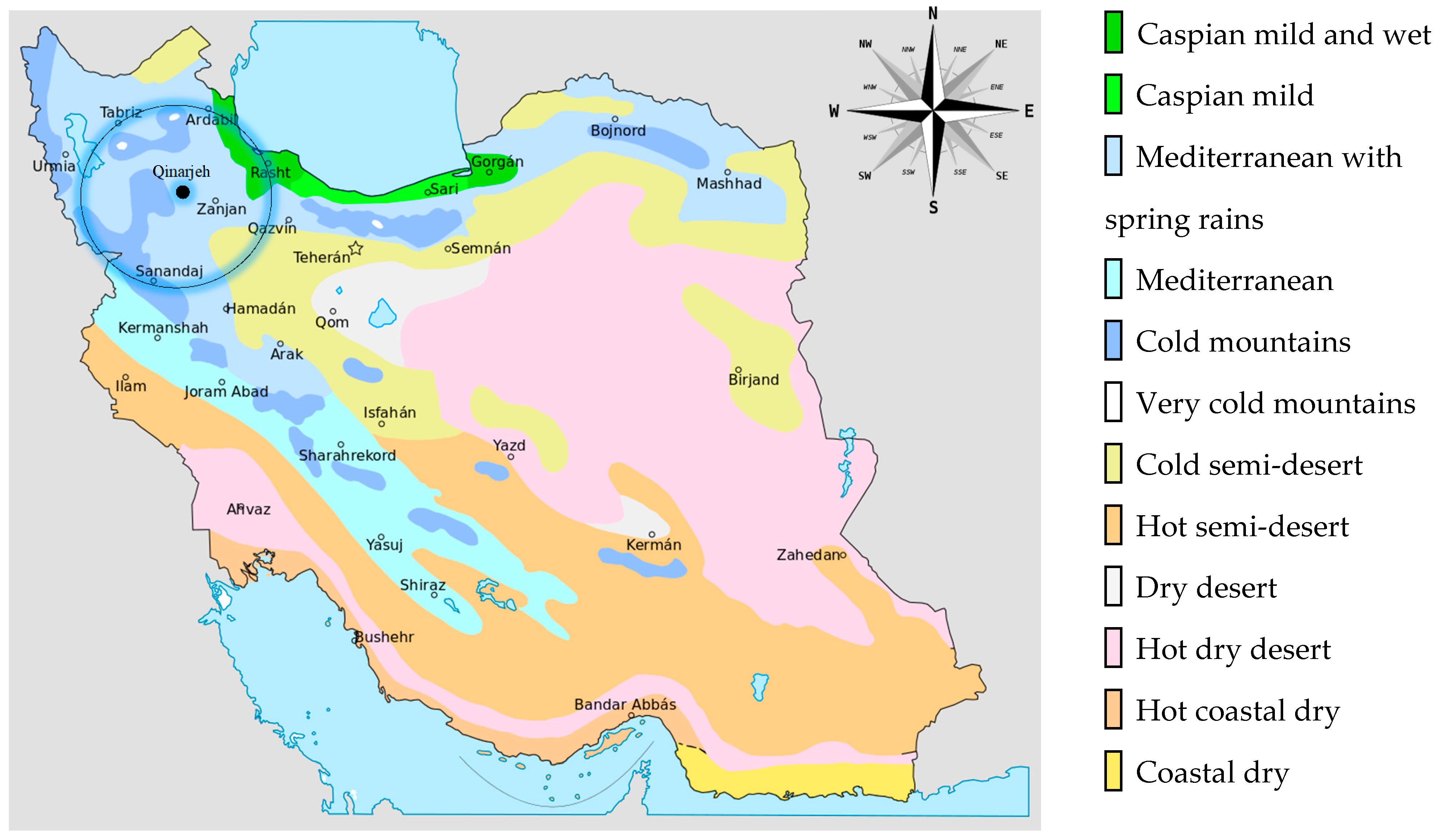
Iran has vast and variable climate regions. Classification of these regions is reported in Figure 1. In the north-west, winter is severely cold with heavy snowfall and subfreezing temperatures during December and January. In addition, spring and fall are relatively mild, while summers are dry and hot.

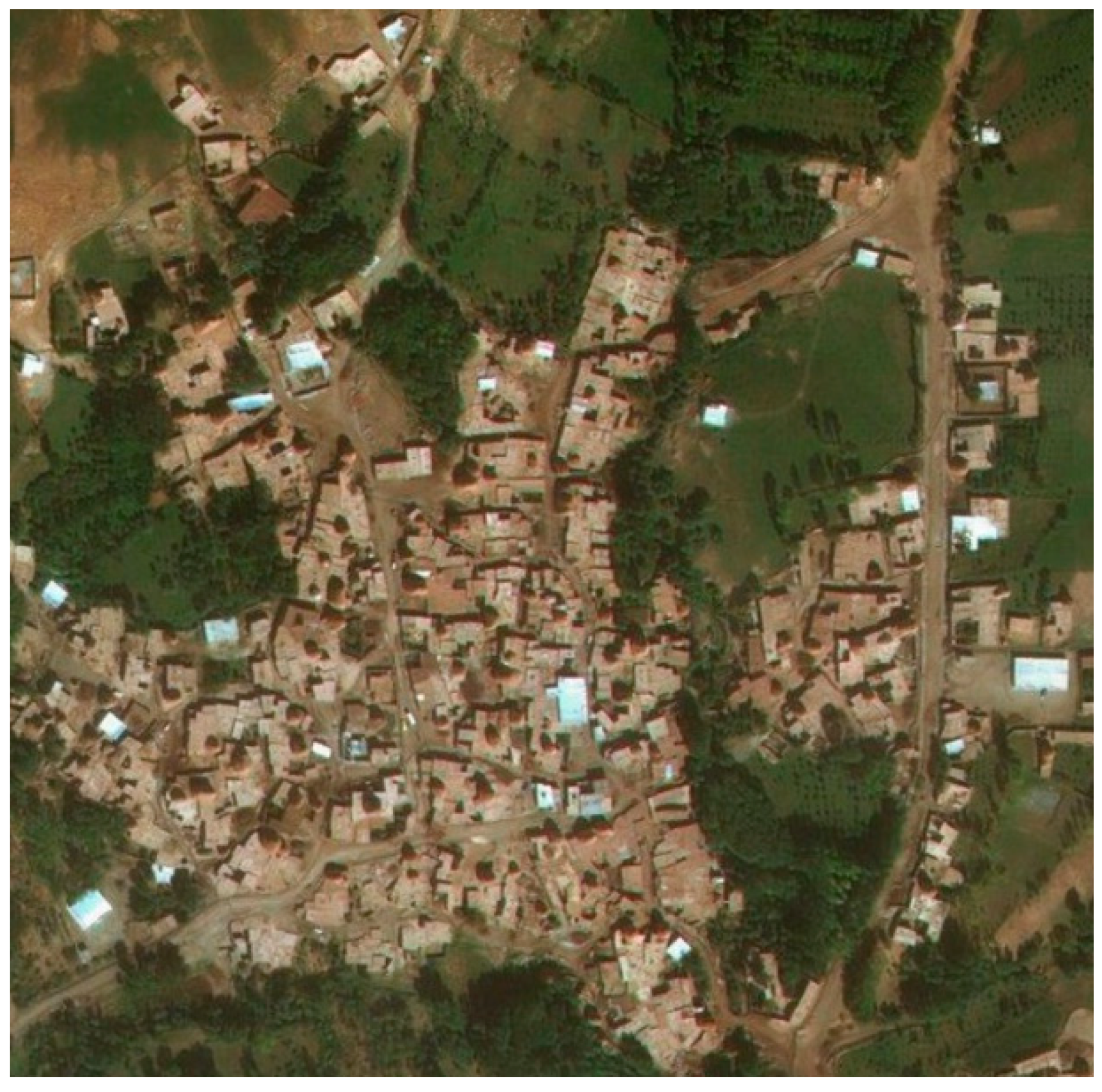
The case study in this research is Qinarjeh village, which is located in the north-west of Iran. According to Figure 2, Qinarjeh is a village near Takab city in West-Azerbaijan province of Iran. The altitude of this region is 2216 m above sea level, which can be classified as a cold mountain climate.

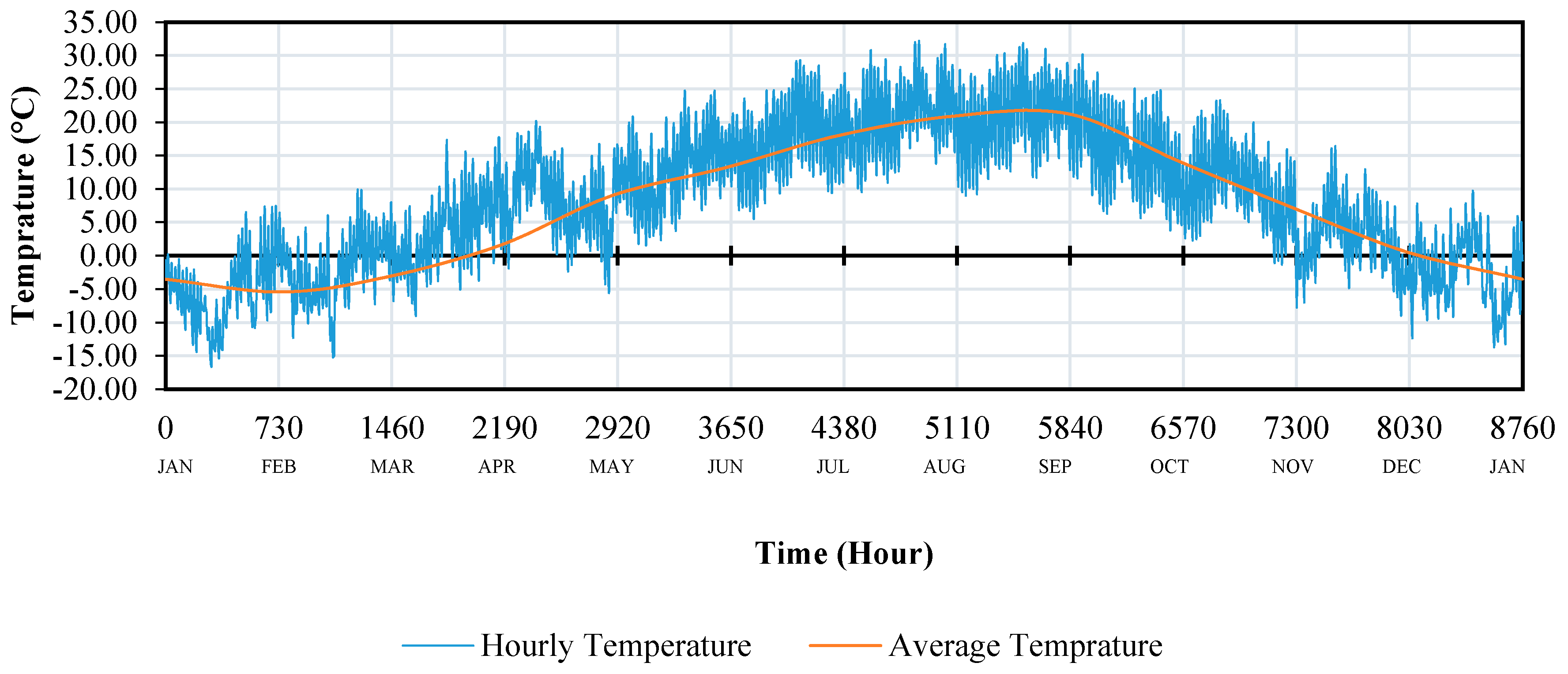
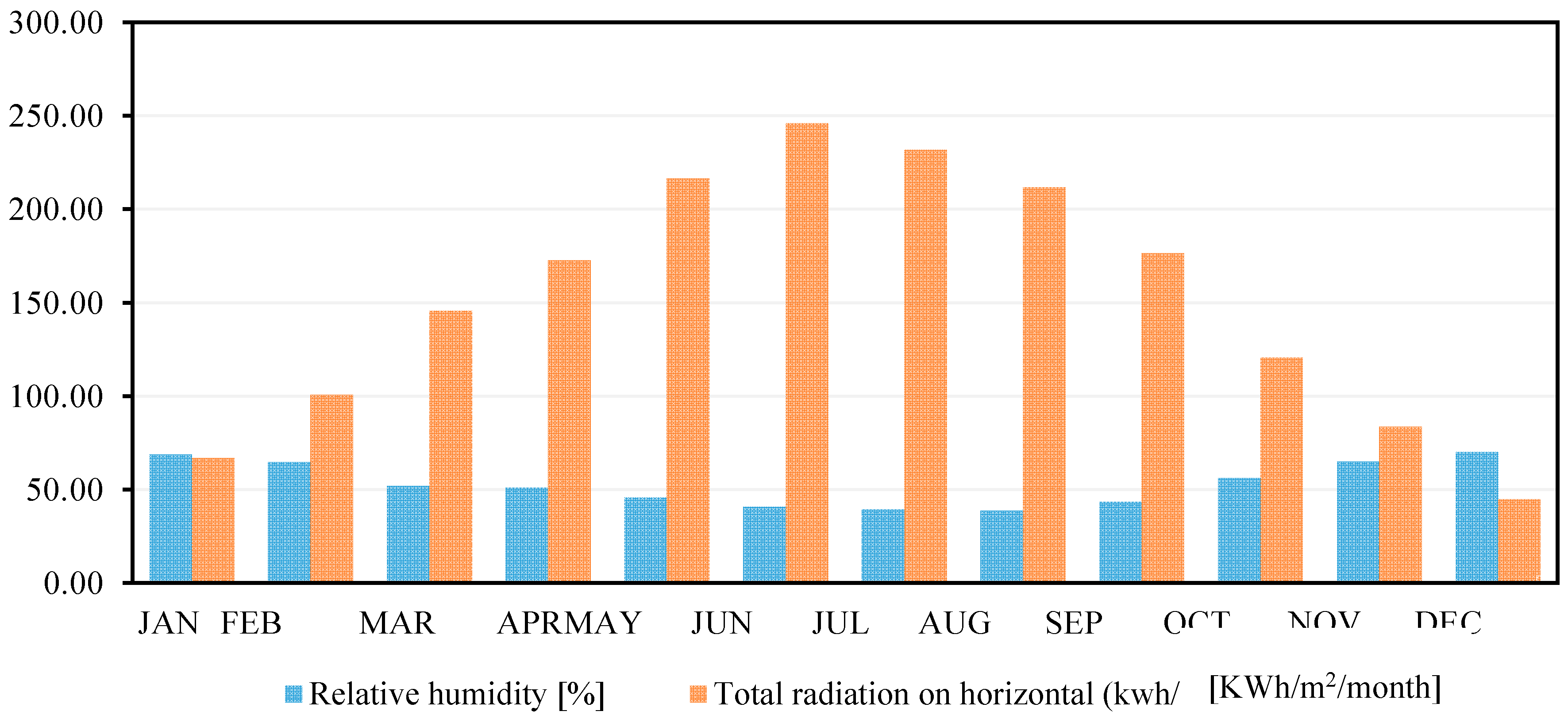
Weather information for this region has been obtained from the climate meteorological data for the years between 2000 and 2010. For this region, hourly and average ambient temperature changes are presented in Figure 3. According to this figure, the minimum and maximum ambient temperatures are −16 °C in January and 32 °C in July, respectively. The average monthly Relative Humidity (RH) (%) and the total radiation on the horizontal ground surface (kWh/m²/month) are presented in Figure 4.

2.2. Future Weather Data Projection

Based on the Intergovernmental Panel on Climate Change (IPCC) data extracted from 2007, four different storylines have been defined to predict the average global temperature increases. These storylines can be classified as average global temperature increases of 1.8 °C, 2.8 °C, and 3.4 °C for the low (B1), medium (A1B), and high (A2) under different CO₂ emission scenarios, respectively, by the year 2100 s [18]. The B1 storyline and scenario family describes a convergent world with the same global population. In this scenario, the global population peaks in mid-century and declines thereafter, with a rapid change in economic structures toward a service and information economy. This results in reductions of material intensity and the introduction of clean and resource-efficient technologies [18]. The A1B scenario family describes a predictive future world with very rapid economic growth. This scenario also proposes the global population peaks in mid-century, which is balanced and does not rely too heavily on one particular energy source. The A2 scenario describes a very heterogeneous world, which is self-reliant and conservative to keep local identities. In this scenario, fertility patterns across regions converge and are very slow, which results in continuously increasing population growth. It means that economic development is regionally-oriented. Moreover, economic growth and technological change per capita are more fragmented and slower compared to other storylines. Accordingly, the researchers believe this trend is more probable for the growth and technological development of the earth. Therefore, for the future weather projection in this paper, the A2 scenario has been followed. In this research, temperature variances of the periods 2020, 2030, and 2040 are used for the calculation of future periods based on the A2 scenario as is illustrated in Figure 5. These weather data are estimated by the extracted data from IPCC HADCM3 (Hadley Center Coupled Climate Model).

HADCM3 makes use of the location of a place or city, along with the world CO₂ emission scenario to deduce the climate change pattern. For this study, a morphing tool [19] named “Climate change world weather generator” is used to produce the future (until 2050) weather profiles. This tool applies the HADCM3 interpolated parameters onto the grid of the local points by using the typical meteorological year (TMY) datasets of the respective region. The average monthly temperature until the 2050 s is presented in Figure 5d. According to this, the amount of temperature increase is 2.31 degrees from 2010 to 2050.

2.3. Village Heating Load

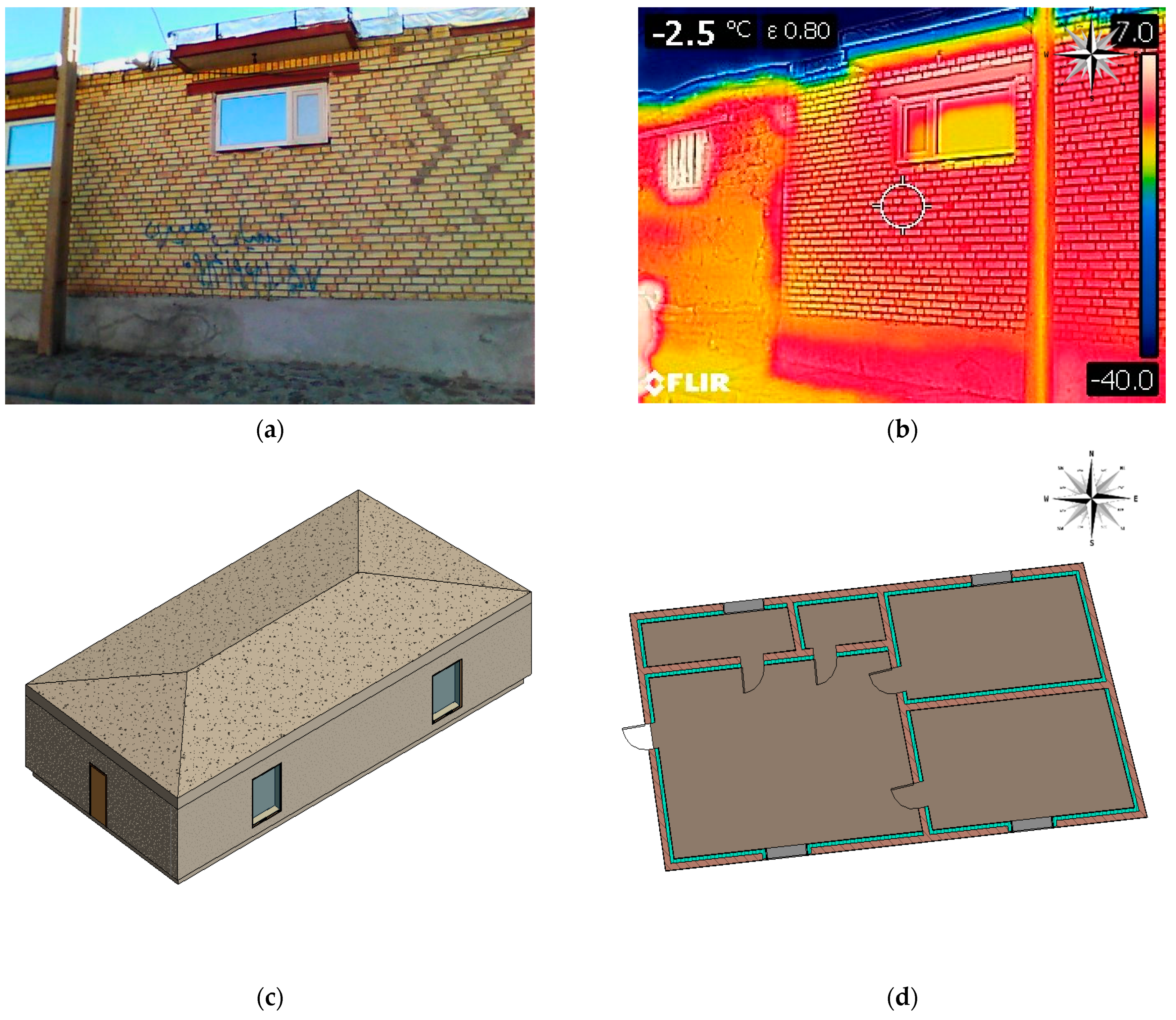
Because of different structures of the rural buildings and variety of building plans for estimating the total heat load of buildings in Qinarjeh village, a sample building, as depicted in Figure 6, has been selected. The building specifications are presented in

Table 1. Sample building specifications.

Area (m2)	U-Value (W/m2K)	Thickness/Property	Orientation	Material
50.4	1.937	0.1 m	NNW	Exterior Wall-1
27.6	1.937	0.1 m	WSW	Exterior Wall-2
50.4	1.937	0.1 m	SSE	Exterior Wall-3
29.2	1.937	0.1 m	ENE	Exterior Wall-4
161	1.148	0.305 m	Horizontal (10% SLOPE)	Roof
161	1.053	0.6m	Horizontal	Floor
2	5.455	0.2m	WSW	Door
2	5.68	Single layer G-value(0.85)	SSE	Window-1,2
2	5.68	Single layer G-value(0.85)	NNW	Window-3,4

, and also the thermophysical properties of the materials used in buildings are given in Table S1 (Supplementary Materials). Moreover, for the initial temperature approximation, and measuring the heat losses, the temperature contours are extracted by a FLIR Thermal camera. After obtaining the heat loss of the sample building per unit area, according to Figure 7, by calculating the number of total areas of the buildings, the entire heat losses of buildings are estimated. Based on the field visits, only 33 percent of the total areas needs heating, and the rest are used as barns and stalls. Accordingly, the total heat losses can be obtained by the multiplication of the sample building load into 33 percent of the total areas, which is calculated as 25,052 square meters.

After calculation of the heating load for the village, it is essential to calculate the building heating load. The building heating load is calculated by following the method, which is presented in the Annex 49 development plan [20]. The heating load is based on the building characteristics, the local climate, and the pattern of users. In this way, the heating load ${\dot{Q}}_{Heat}$, results from the imbalance between energy losses, ${\dot{Q}}_{Losses}$, (transmission, ${\dot{Q}}_T$, ventilation and infiltration, ${\dot{Q}}_V$) and energy gains, ${\dot{Q}}_{Gain}$, (solar gains, ${\dot{Q}}_S$, and internal gains, ${\dot{Q}}_I$), which can be calculated by the following equations [21].

$${\dot{Q}}_{Heat}={\dot{Q}}_{Losses}-{\dot{Q}}_{Gain}$$

(1)

$${\dot{Q}}_{Losses}={\dot{Q}}_T+{\dot{Q}}_V$$

(2)

$${\dot{Q}}_{Gain}={\dot{Q}}_S+{\dot{Q}}_{I,o}+{\dot{Q}}_{I,e}+{\dot{Q}}_{I,L}$$

(3)

Transmission heat loss (${\dot{Q}}_T$) is the sum of the heat loss from all external walls, doors, windows, roof, and floor [8].

$$\begin{array}{c}{\dot{Q}}_T={\dot{Q}}_{Window}+{\dot{Q}}_{Door}+{\dot{Q}}_{Wall}+{\dot{Q}}_{Roof}+{\dot{Q}}_{Floor}\\ {\dot{Q}}_T=\sum \left(U_i\times A_i\times F_{x,i}\right)\times \left(T_i-T_e\right)\end{array}$$

(4)

In the above-mentioned formula, $T_i$ and $T_e$ are the indoor and outdoor temperatures, respectively. In Equation (4), $F_{x,i}$ represents the temperature correlation factor, which is set to one according to the regulations for the exterior walls and roofs and to 0.6 for the floors that are facing the ground [8].

Ventilation heat loss (${\dot{Q}}_V$) is obtained by the following relation.

$${\dot{Q}}_V=\sum \left(C_p\times n_d\times V\right)\times \left(T_i-T_e\right)$$

(5)

where V represents the overall building volume, $n_d$ represents the air exchange rate, and $C_p$ represents the specific heat capacity of air with the value of 0.34 [Wh/(m³ K)] [8].

Similar to the heat losses, the heat gains need to be calculated. They are subdivided into two categories: solar and internal heat gains. To calculate the solar gains, the following equation has been used.

$${\dot{Q}}_S=\sum \left(I_{S,j}\times A_{W,i}\times g_{L,i}\times F_{F,i}\times F_{W,i}\times F_{C,i}\times F_{S,i}\right)$$

(6)

Four correction factors in Equation (6) consider possible shading by shading devices (F_C), surrounding buildings (F_S), nonorthogonal solar radiation (F_W), and window framing (F_F).

The internal heat gains (${\dot{Q}}_{I,o}$) in the residential buildings are different from the internal gains in office and administration buildings. The internal loads are higher in the office buildings because of the office equipment. The heat gain per person (${\ddot{Q}}_{I,o}$) is set to a mean value of 100 W, and then multiplied by the statistic number of occupants ($n{o}_o$).

$${\dot{Q}}_{I,o}={\ddot{Q}}_{I,o}\times n{o}_o$$

(7)

To simplify the input parameters, the specific heat gain by the electrical appliances (${\ddot{Q}}_{I,e}$) was set as static value for all rooms. Then, it is multiplied with the room area ($A_n$) according to the following equation.

$${\dot{Q}}_{I,e}={\ddot{Q}}_{I,e}\times A_n$$

(8)

Other uses, like lighting, are considered as extra internal gains. It is assumed that the electricity demand for lighting turns into internal heat loads inside the building and specific lighting power ($P_{Li}$) is considered as a constant value of 20 [W/m²] [22].

$${\dot{Q}}_{I,L}=P_{Li}\times A_n$$

(9)

2.4. Total Boiler Heating Load

In order to calculate the total boiler heating load, it is necessary to first calculate the heat losses of the equipment, piping, and DHWS, which has been studied in this section.

2.4.1. Boiler Heat Losses

For boiler heating load calculations, it is assumed that the respective heat for such DH system is provided by the boilers, which use the natural gas as the fuel due to the availability of such boilers in Iran. Then, the inlet fluid temperature ($T_{in}$) and the set-point temperature ($T_{set}$) are considered to be 72 °C and 82 °C, respectively. The reason for choosing these temperatures is that the heating devices in the buildings are radiators that work effectively within these temperature conditions. Then, a boiler is defined by its overall (output/input) and combustion efficiencies. Therefore, the energy loss during the combustion process can be calculated by integrating the following equations [11,23].

$${\dot{Q}}_{fluid}={\dot{m}}_{fluid} C_{P fluid} \left(T_{set}-T_{in}\right)$$

(10)

$${\dot{Q}}_{fuel}=\frac{{\dot{Q}}_{fluid}}{{\eta }_{boiler}}$$

(11)

$${\dot{Q}}_{exhaust}={\dot{Q}}_{fuel} \left(1-{\eta }_{combustion}\right)$$

(12)

where $C_{P fluid}$ is the specific heat of liquid and assumed to be 4.18 [kJ/(kgK)] [24]. In such equations, ${\dot{Q}}_{fuel}$ is the rate at which the fuel is consumed. In Equations (11) and (12), ${\eta }_{combustion}$ and ${\eta }_{boiler}$ are the combustion efficiency of boiler and the overall efficiency, respectively, which are assumed to be 0.85 and 0.78, respectively, and have been obtained from commercial products.

2.4.2. Piping Heat Losses and Pump Power Calculation

The overall piping plan for such a village according to the building densities and the main road lines is depicted in Figure 8. Such design is adapted to cross the main flat connecting roads inside the village, to reduce the number of loops and the construction costs. According to this sketch, supply and return of the main pipelines are a closed loop system with about 2047 m length from the central powerhouse. Sub-branches have 43 lines with ~20 m lengths. In the main pipeline, a constant pressure drop limit of 2.5 to 4% for each 100 m length of the pipe is considered [3,23]. For calculating the diameter of the pipelines, the volumetric flow rate is determined based on the density of house areas to supply on each line as is shown in

Table 2. Pipeline specifications.

Pipeline	Length (m)	Flow Rate [%]
Line 1	132	100
Line 2	102.1	49.0
Line 3	76.2	51.2
Line 4	741.7	28.0
Line 5	230.8	21.0
Line 6	226.6	14.0
Line 7	176.2	7.0
Line 8	92.7	7.0
Line 9	191.0	14.0
Line 10	77.9	9.3
Sub-Branches	43 × 20	2 (For each branch)

.

The diameter of the pipe ($D$) is obtained from the Hazen–Williams equation [23], which is defined according to the following equation.

$$\Delta h=3.022L\times (\frac{V}{C}{)}^{1.852}\times (\frac{1}{D}{)}^{1.852}$$

(13)

By replacing the velocity variable ($V$) with a volumetric flow rate ($\dot{V}$) in Equation (14), the diameter of the pipe can be calculated by the following equation [23].

$$D=\sqrt[-4.871]{\frac{\frac{\Delta h}{L}}{4.727\times (\frac{\dot{V}}{C}{)}^{1.852}}}$$

(14)

where C is the roughness factor and is considered to be 140 for the new steel pipe [23], $\dot{V}$ is the volumetric flow rate, and $\Delta h$ is the head losses.

For this study, the centrifugal water pump is considered where the overall pump and motor efficiencies are extracted from the commercial centrifugal performance curves, which are set as 0.6 and 0.9, respectively. The power required to drive the pump (P_i), is defined by the following equations [25].

$${\dot{P}}_i=\frac{\rho gh\dot{V}}{{\eta }_{pumpimg}}$$

(15)

$${\dot{P}}_{total}=\frac{{\dot{P}}_i}{{\eta }_{motor}}$$

(16)

where ${\dot{P}}_i$ is the power of the pump shaft and ${\dot{P}}_{total}$ is the total power drawn by the pump, which includes the effects of motor inefficiency. In Equations (15) and (16), ${\eta }_{pumpimg}$ is the overall pump efficiency and ${\eta }_{motor}$ is the motor efficiency. The energy transferred from the motor to the ambient is given by the following equation [23,25].

$${\dot{Q}}_{loss,pump}=({\dot{P}}_{total}-{\dot{P}}_i)\times \left(1-f_{motorloss}\right)$$

(17)

where $f_{motorloss}$ is a value between 0 and 1 that determines whether the motor inefficiencies cause a temperature rise in the fluid stream that passes through the pump or whether they cause a temperature rise in the ambient air surrounding the pump. Because the motor is assumed to be kept outside of the fluid stream, so the waste heat of the motor impacts the ambient, and $f_{motorloss}$ would have a value of 0.

Heat losses of the piping can be calculated by integrating the following equation [10,26,27].

$$d{Q}_{loss,piping}=\frac{1}{R_{total}} \left(T_{fluid}-T_{soil}\left(\mathrm{z},\mathrm{t}\right)\right)\mathrm{dx}$$

(18)

where $T_{fluid}$ represents the temperature of the circulating fluid and $T_{soil}$ is the soil temperature which changes with the time and the depth under the ground and can be calculated by the following equation.

$$T_{soil}\left(\mathrm{z},\mathrm{t}\right)=T_{ms}+A_s{e}^{-z\sqrt{\frac{\pi }{\alpha \zeta }}}\sin (\frac{2\pi (t-t_{lag})}{\zeta }-\mathrm{z}\sqrt{\frac{\pi }{\alpha \zeta }})$$

(19)

where $T_{ms}$ is the mean annual surface temperature, α is the thermal diffusivity of the soil, A_s is the surface temperature amplitude, and $\zeta$ is the annual period length, which is considered as 365 days for a whole year. Resistance values are obtained by the following equations.

$$R_{total}=R_{fluid}+R_{pipe}+R_{insulate}+R_{backfill}$$

(20)

$$R_{fluid}=\frac{1}{h_{conv} A_{surf}}$$

(21)

where in the above-mentioned equation $R_{fluid}$ is the resistance of fluid, $R_{pipe}$ is the resistance of pipe, $R_{insulate}$ is the resistance of insulation, and $R_{backfill}$ is the resistance of backfill. The convective heat coefficient ($h_{conv}$) is obtained from the following equations [28,29].

$$h_{conv}=\frac{Nu\times k_{fluid}}{D_{in}}$$

(22)

$$N{u}_D=0.023\times R{e_D}^{\frac{4}{5}}\times P{r}^{0.3}$$

(23)

where Nu represents the Nusselt number, $Pr$ is the Prandtl number, and k_fluid represents the fluid thermal conductivity. Properties of the water flow at the set point temperature is determined from Holman [29] as are presented in

Table 3. Water flow properties.

Parameter	Value
Pr	2.39
k	0.673 (W/(m·°C))
µ	3.47 × 10−4 (kg/(m·s))

.

According to the pipe shape in cylindrical coordinates, the resistance values of the pipe, insulation, and backfill are obtained from the following equation [27,30].

$$R=\frac{ln(\frac{r_{outer}}{r_{inner}})}{\pi K \mathsf{\Delta }z}$$

(24)

where K is the total thermal conductivity of the pipe, insulation, and backfill. For more details, it is noteworthy to mention that, for this study, elastomeric type of insulation with a thermal conductivity of 0.0353 (W/(m K)) is considered and thermal conductivity of the backfill is assumed to be 2.42 (W/(m K)) [30].

2.4.3. Domestic Hot Water Supply (DHWS)

For designing the DHWS in the first step, the hot water demand is needed. In the second step, the population data is needed. Based on the population census data and the usage of hot water per person the total number of residents for the DHWS network is counted as 854 people. In the third step, because the exact numbers of fixture units were unclear, the American Society of Plumbing Engineers (ASPE) [31,32] standard method for calculating DHWS flow rate has been used, which is based on the occupant demographic classifications [33]. By referring to this method, the DHW usage is categorized into three groups (low, medium, and high) based on the occupant demographic classifications. The DHW demand within these classifications is presented in

Table 4. Hot water demand and guidelines (adapted from ASPE 2003).

Classifications	Maximum Hourly	Maximum Daily	Average Daily
Low	10.6	75.7	53.0
Medium	18.1	185.4	113.5
High	32.1	340.6	204.4

Unit: L/person.

. Accordingly, the classification of the occupants for the desired village is medium; Table 4 shows the maximum hourly and daily water used for each person as 18.1 and 185.4 L, respectively.

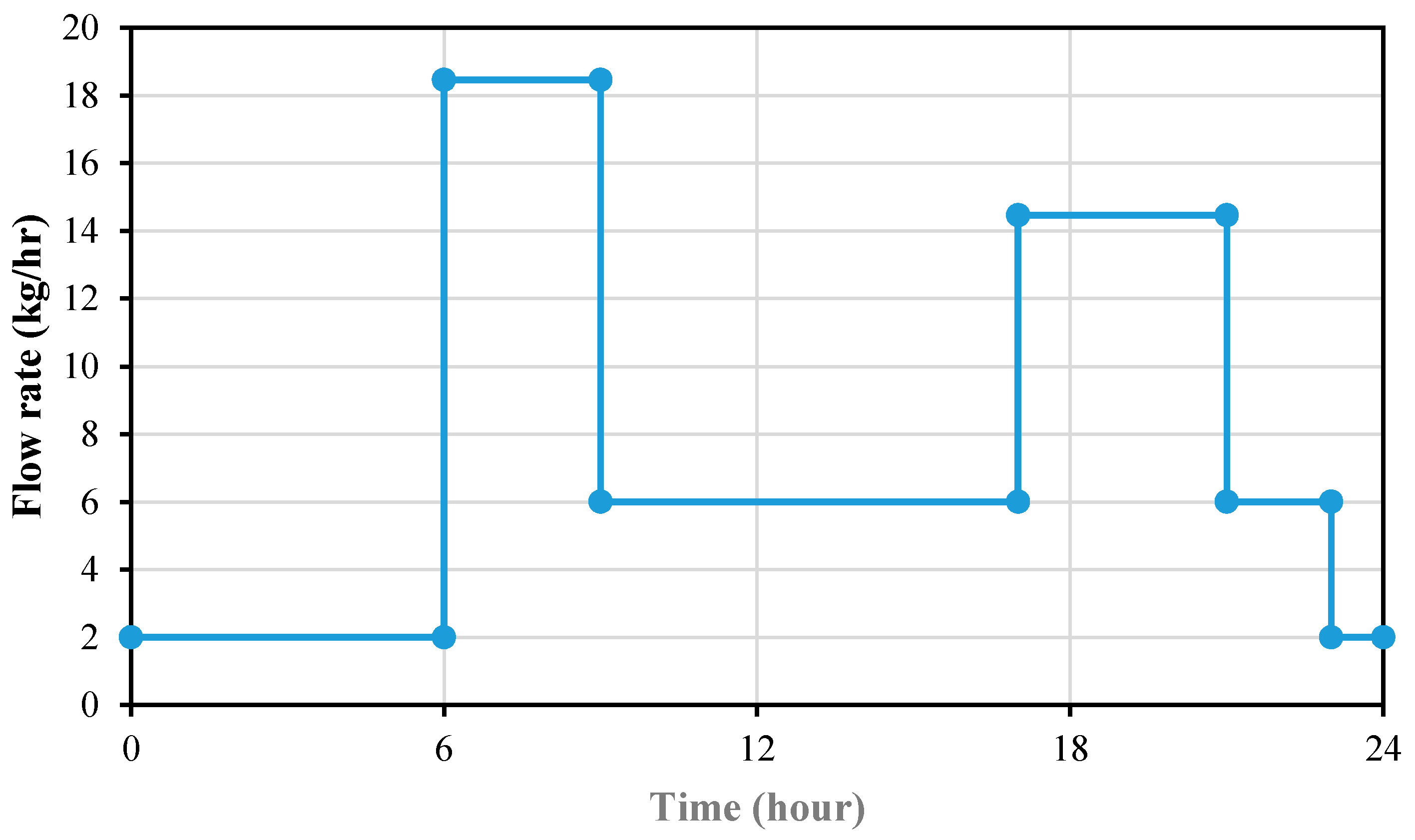
For calculating DHW load, a possibility assumption profile of daily water used for each person is presented in Figure 9, which perfectly satisfies the conditions of Table 3.

Then the DHW load can be calculated by the following equation.

$${\dot{Q}}_{DHW}={\dot{m}}_{fluid}\times 4.19\times \left(T_{set}-T_{in}\right)$$

(25)

where the value of 4.19 represents the specific heat of the water, T_set and T_in are 60 and 10 °C, respectively.

In this study, heat losses of the valves and other equipment are ignored so that the total boiler heating load can be calculated by the following equation.

$${\dot{Q}}_{boiler}={\dot{Q}}_{Heat}+{\dot{Q}}_{DHW}+{\dot{Q}}_{loss,boiler}+{\dot{Q}}_{loss,pump}+{\dot{Q}}_{loss,piping}$$

(26)

3. Life Cycle Cost (LCC)

In this research, the LCC is used to consider the costs that are involved in the design of the DH system. These costs are classified as the initial cost, the present value of the energy, and gas price for a 30 year-period.

The life cycle cost includes accumulated investment and operation costs. The annual maintenance cost for the equipment and salvage cost at the end of its useful life is not considered in this study. It has been excluded because of the lack of accurate data about them. Additionally the most effective parameters for the optimization of the LCC are the investment costs, fuel costs, escalation, and discount rate. Accordingly, the investment costs include insulation material, boiler, radiators, pumps, heating supply pipelines, and pipe insulations costs. It should be noted that the boiler and pumps costs are affected by changing the insulation material. By insulating the building envelope, the heating load demand decreases, and a smaller boiler, pump, and radiator can be selected. Moreover, the diameter of the heating supply pipelines would be smaller and finally, the total costs of pipes and insulations of the pipelines would be less. Therefore, the total investments design would decrease drastically. Operation cost includes gas consumption of the boiler and electricity consumption of pumps over the system life cycle. The complete approach to economic analysis is to use the LCC method that takes into account all future expenses. Such a complete approach provides a mean for comparison of the future costs with today’s prices. For this purpose, the present value of the fuel cost is used. Therefore, the life-cycle cost (LCC) can be calculated by the following equations, which is considered for a 30-year period [34,35].

$$\mathrm{LCC}\left(30 \mathrm{years}\right)=\mathrm{IC}+{\mathrm{PV}}_{\mathrm{electricity}}+{\mathrm{PV}}_{\mathrm{gas}}$$

(27)

$$IC=I{C}_{boiler}+I{C}_{building insulation}+I{C}_{radiators}+I{C}_{pump}+I{C}_{pipes}+I{C}_{pipes insulation}$$

(28)

where $IC$ represents the investment costs and PV represents the present value of the energy for 30 years which can be calculated by the following equation [34]:

$$PV=\sum _{n=1}^{30}(Cos{t}_{annual}\times \frac{{\left(1+ESC\right)}^n}{{\left(1+DIS\right)}^n})$$

(29)

$$DIS=di{s}_{nominal}-\mathrm{inflation} \mathrm{rate}$$

(30)

where ESC is the escalation rate of the energy cost, which is considered as 8.3% for each year, and $DIS$ is the real discount rate, which is assumed to be 3% for each year. The amount of escalation rate is chosen according to the Iranian national data because all investment and the fuel costs must be converted to USD to be comparable with a global scale. So, the discount rate is obtained from the US federal estimation for the year 2019.

4. Optimization

For optimizing the proposed DH system of the Qinarjeh village, it is needed to perform several steps. In the first step, the role of different building insulation types and layers from the economic and environmental points of view should be studied. It means that, for such an evaluation, a fixed retrofit version of residential buildings must be found to perform the general system optimization.

4.1. Building Retrofit

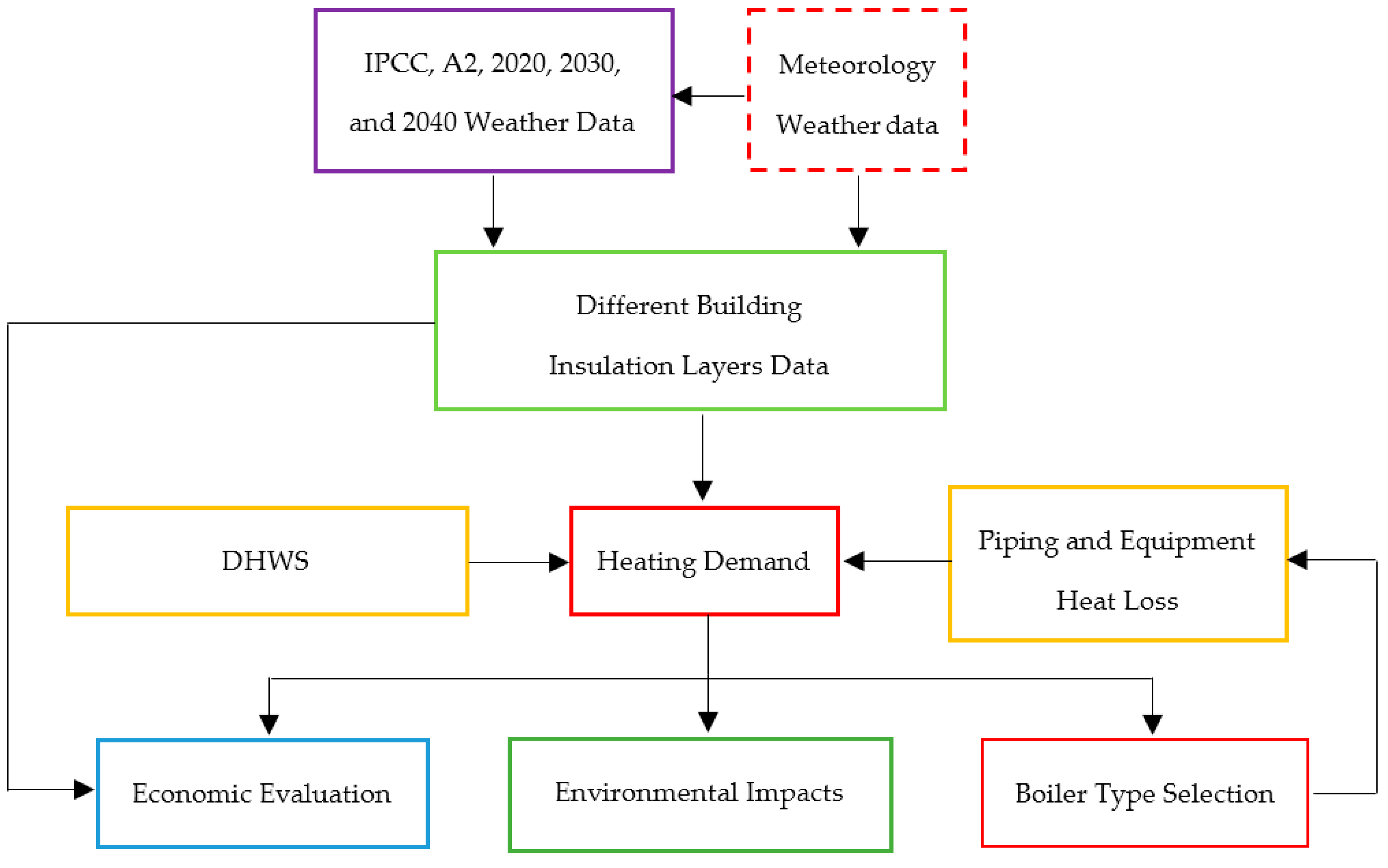
For finding the best material to minimize the heat losses from the building some measures have been performed. A building retrofit study has been proposed to minimize the heat losses from the residential buildings. One of the most effective ways to reduce heat losses is to insulate the building envelope. The flowchart in Figure 10 illustrates the procedures performed to evaluate each retrofit scenario. Such a flowchart is designed to investigate the effect of different building insulation layers on the desired DH system by considering the economic and environmental impacts. Therefore, a Fortran code is developed according to the depicted algorithm presented in Figure 10.

To fulfill the required input parameters for all the studied insulation materials,

Table 5. Different insulation types and layers.

Case Number	Exposure (sides)	Insulation Material	Density (kg/m3)	Thickness (m)	U (W/(m·K))	Total Price/m2·($)
1	Wall	Polystyrene eps	20	0.05	0.042	5.56
2		Polystyrene eps	20	0.1	0.042	8.33
3		Polystyrene xps	32.97	0.05	0.0302	7.64
4		Polystyrene xps	32.97	0.1	0.0302	12.50
5		Polyurethane	30	0.05	0.02	12.78
6		Polyurethane	30	0.1	0.02	22.78
7		Rockwool	100	0.025	0.044	5.83
8		Rockwool	100	0.05	0.044	8.89
9		Glass wool	50	0.025	0.038	4.31
10		Glass wool	50	0.05	0.038	5.58
11		Glass wool	100	0.025	0.039	5.58
12		Glass wool	100	0.05	0.039	8.39
13	Ceiling	Polystyrene eps	20	0.05	0.042	5.56
14		Polystyrene eps	20	0.1	0.042	8.33
15		Polystyrene xps	32.97	0.05	0.0302	7.64
16		Polystyrene xps	32.97	0.1	0.0302	12.50
17		Polyurethane	30	0.05	0.02	12.78
18		Polyurethane	30	0.1	0.02	22.78
19		Rockwool	100	0.025	0.044	5.83
20		Rockwool	100	0.05	0.044	8.89
21		Glass wool	50	0.025	0.038	4.31
22		Glass wool	50	0.05	0.038	5.58
23		Glass wool	100	0.025	0.039	5.58
24		Glass wool	100	0.05	0.039	8.39
25	Window	PVC (0.71 G_value)	-	Double layer	3	28.33
26		PVC (0.71 G_value)	-	Triple layer	2.2	38.33

is presented. Table 5 shows the collected data for different kinds of insulation layers. Such types and thicknesses of layers are extracted from the common insulation products for the building purposes in Iranian companies.

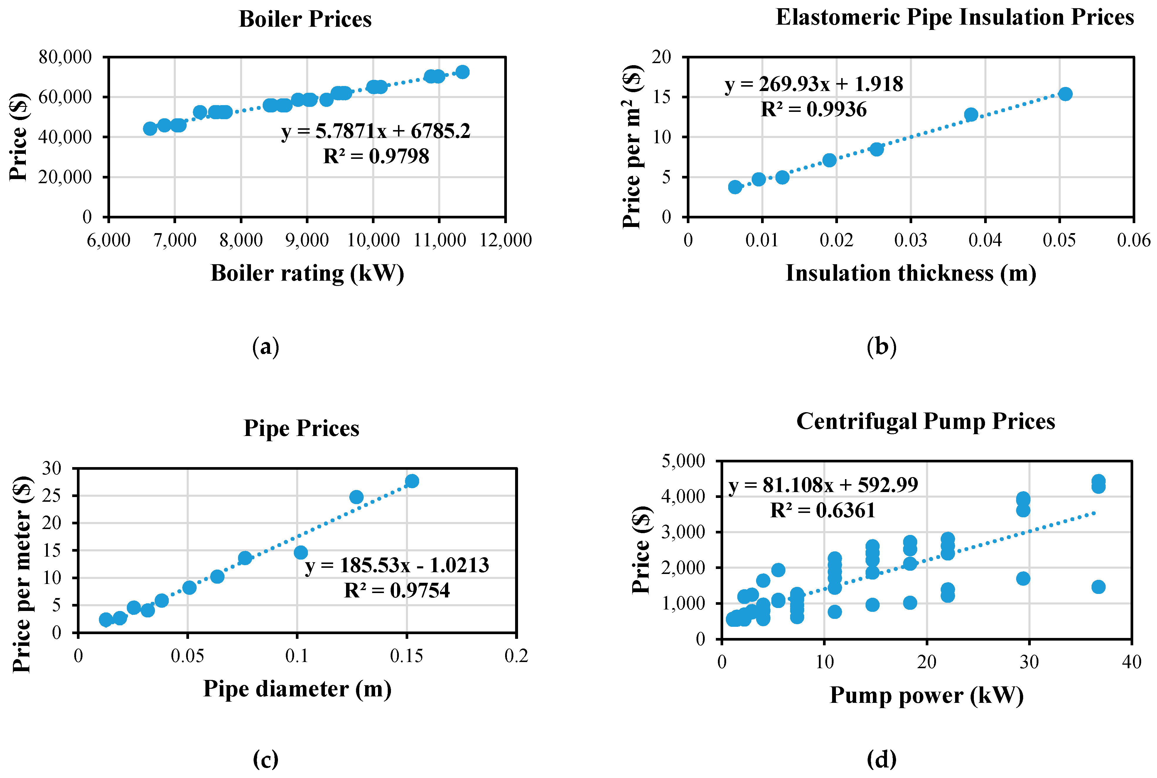
Other input parameters are the economic ones, which are mainly reported in dollar currency for the present study. For convenience calculating of the prices of the equipment, the curve fitting equations of the prices extracted from the commercial products are presented in Figure 11.

For considering the economic and environmental effects of fuel on the designed DH system, several parameters, such as CO₂ emission, fuel consumption, and fuel prices, can be accounted. Due to the availability of natural gas sources in Iran and the operation of heating equipment, mainly by this kind of fuel, natural gas input parameters are extracted from

Table 6. Natural gas properties.

Fuel Type	Specific Fuel Energy		Specific CO2 Emission
Methane (natural gas)	kWh/kgfuel	Btu/ft3	kgCO2/kgfuel	kgCO2/kWh
	15.4	983	2.75	0.18

[36]. Annual gas consumption and CO₂ emission can be determined by having the total heating load demand, specific fuel energy, and specific CO₂ emission.

4.2. General System Optimization

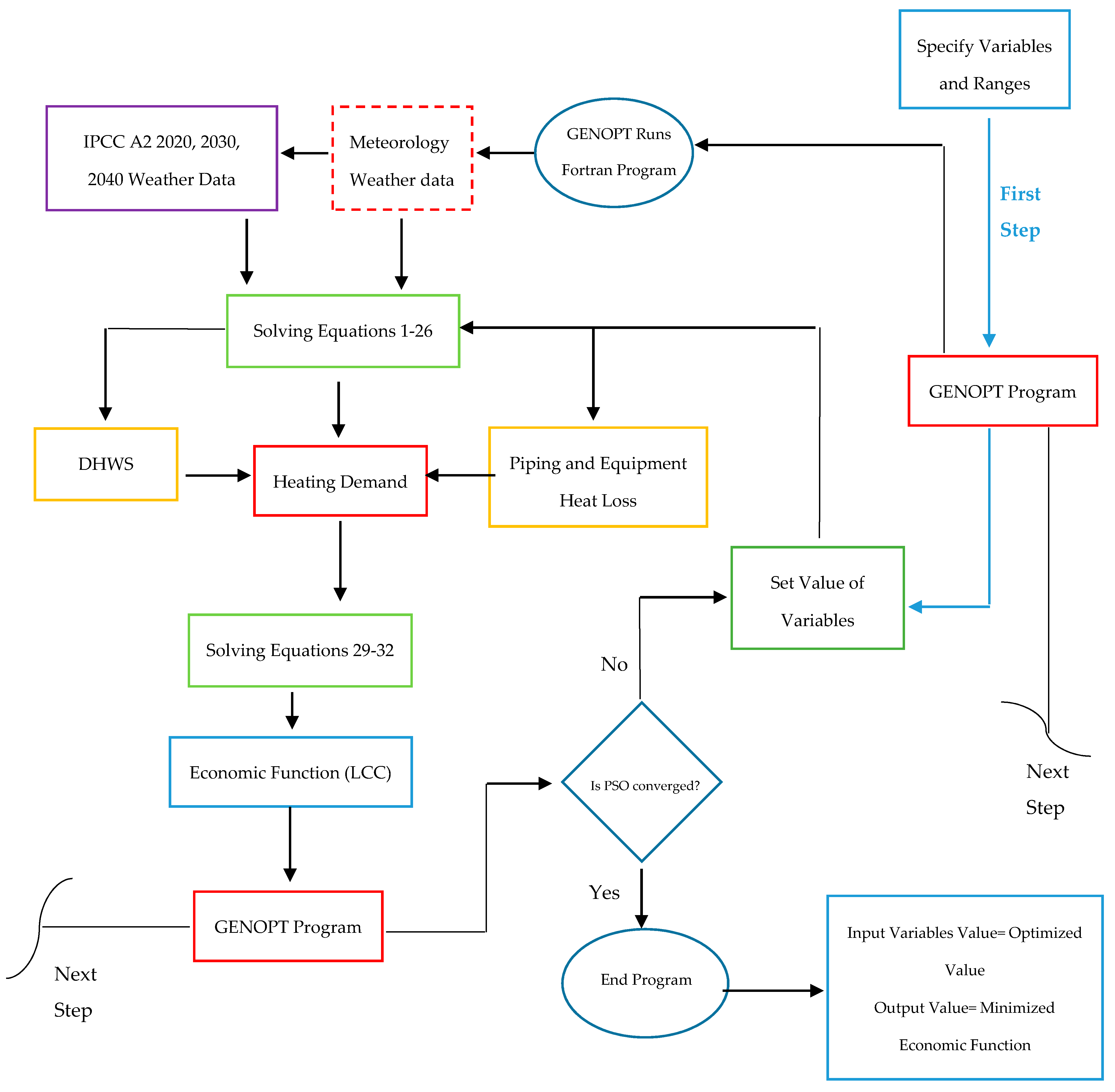
After the selection of the optimum retrofit scenario, general system optimization is performed. Six parameters, including ceiling insulation thickness, wall insulation thickness, pipe insulation thickness, depth of buried heating supply pipes, depth of DHWS pipes, and outlet boiler temperature, are considered as design variables. The minimum LCC is considered as the objective function. A fixed Particle Swarm Optimization (PSO) method with constriction coefficient was selected for this study. In PSO, the potential solutions are called particles, which fly through the problem space by following the current optimum particle [37]. Every particle could find its best position and the group best position through iteration. It has been indicated that the constriction coefficients increases the rate of convergence; further, these coefficients can prevent explosion and induce particles to converge on local optima [38]. A schematic view of the application of the PSO method for the current investigation is presented in Figure 12.

Parameters values for PSO method has been gained from Almeida et al. [39], as presented in

Table 7. PSO method with constriction coefficient parameters.

Parameter	Value
Neighborhood topology	gbest
Neighborhood size	1
Number of particles	10
Number of generation	10
Seed	20
Cognitive acceleration	0.5
Social acceleration	0.5
Constriction gain	0.5

.

The general optimization of DH system is also performed by considering the climate changes. GENOPT software is used for this work [40]. The selected variables for this optimization and their range of changes are presented in

Table 8. Selected variables range of changes.

Variable	Minimum Value	Maximum Value
Ceiling insulation thickness	0	20 (cm)
Wall insulation thickness	0	20 (cm)
Pipe insulation thickness	0	10 (cm)
Depth of buried heating supply pipes	0	10 (m)
Depth of DHWS pipes	0	10 (m)
Outlet boiler temperature	60	100 (°C)

.

The input temperature of the radiators depends on several parameters such as the output temperature of the boiler, the length of the piping, the thickness of the insulation of the pipes, and the depth of the underground buried pipes. From all the above-mentioned parameters, the most important is the output temperature of the boiler. Iranian radiators are usually built to work at an inlet temperature of 80 °C. The higher temperature at the inlet of the radiator will increase the heat load of the radiator. Therefore, in a fixed heat load for a residential building, the size of the radiator is reduced. For calculation of the total numbers of radiators, the following correction factor that is obtained from the commercial radiator product is multiplied by the total heating demand.

$$F_{radiator}=(\frac{60}{T_O-T_{set}}{)}^{1.2899}$$

(31)

where $F_{radiator}$ is the correction factor, $T_O$ is the inlet temperature to the radiator, and $T_{set}$ is the set-point temperature, which is considered to be 20 °C.

5. Results and Discussion

The results are divided into the heating load demand, insulation selection, environmental impacts, economic analysis, and general optimization analysis sections. In Section 5.1, hourly simulation results of the DH demand with a forecast of future decades by the projection of heat losses of different equipment are presented. In Section 5.2, the effects of insulation selection on the heating demand are calculated. In Section 5.3, the reduction of natural gas consumption by applying the different insulation layers at the sides of buildings and CO₂ emission is estimated. In Section 5.4, the economic analysis of the different insulation layers, initial costs, operation costs, and LCC in 30 years is discussed. Finally, in Section 5.5, the results of the simulation for the general optimization of different variables according to Table 8 with and without considering climate change have been investigated.

5.1. Heating Demand

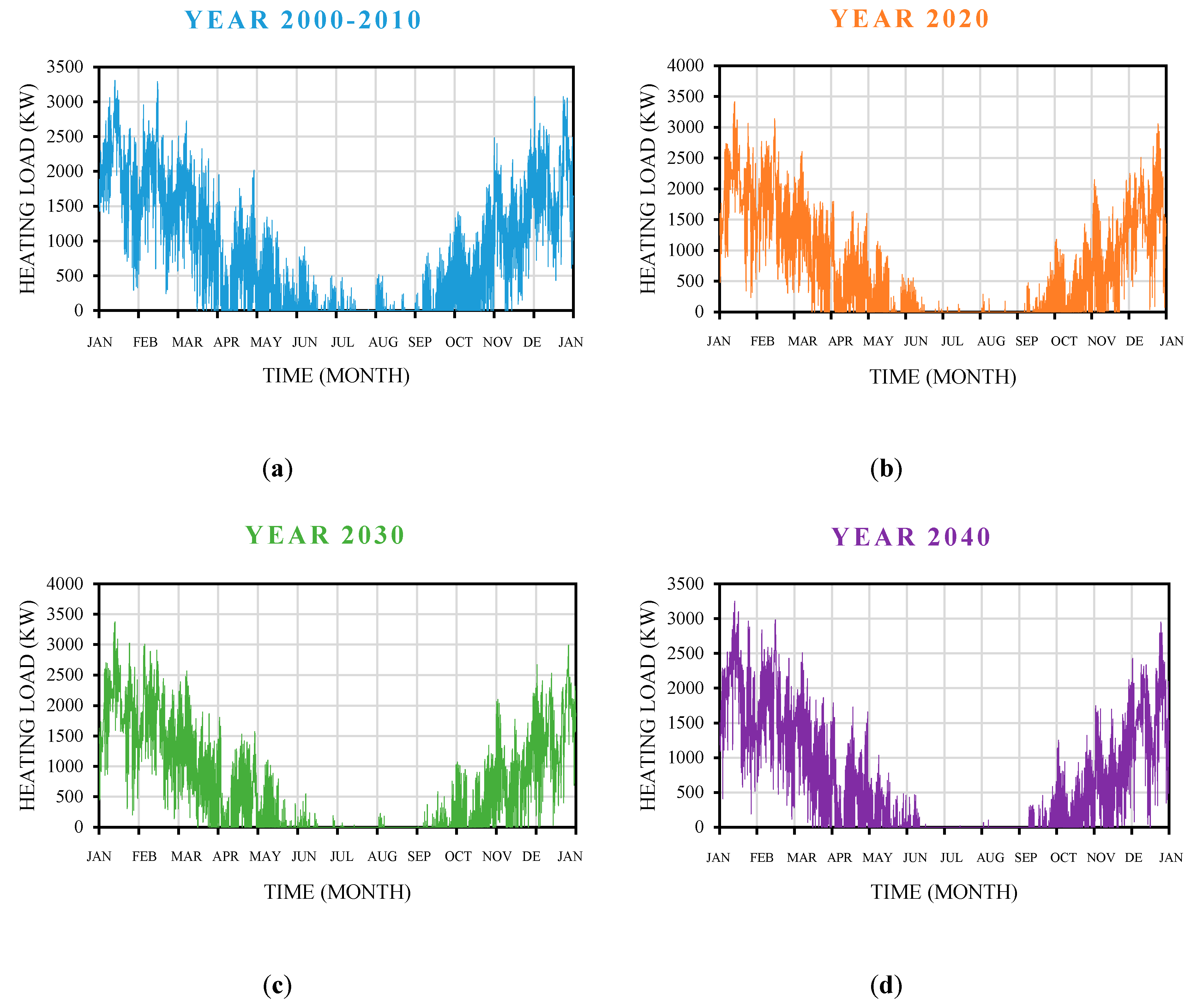
There are two critical factors for the design of the DH system—different types of building insulations and future weather changes—which both can lead to massive changes in energy consumption. Hourly simulation of heating loads of total residential buildings is shown in Figure 13. The results are obtained from hourly temperature, solar radiation, and the projected future data. According to the diagrams, the amount of peak load in the average years between 2000 to 2010 is 3.31 MW and occurs in February. In addition, the peak loads of the years between 2020 to 2040 occur in January. This peak loads for the year between 2020 to 2040, first increase to 3.42 MW and then decrease to 3.25 MW.

5.2. Insulation Selection

According to Figure 14 in future years, the total amount of annual heating load will be decreased because of global warming. Moreover, the minimum heating load belongs to insulation case number 6, which is a polyurethane layer with 10 cm thickness. Also, it can be concluded that the amount of the annual heating load will decrease by 20% until the 2040s. So, in terms of load reduction, polyurethane and Rockwool could be the best and the worst insulation types, respectively.

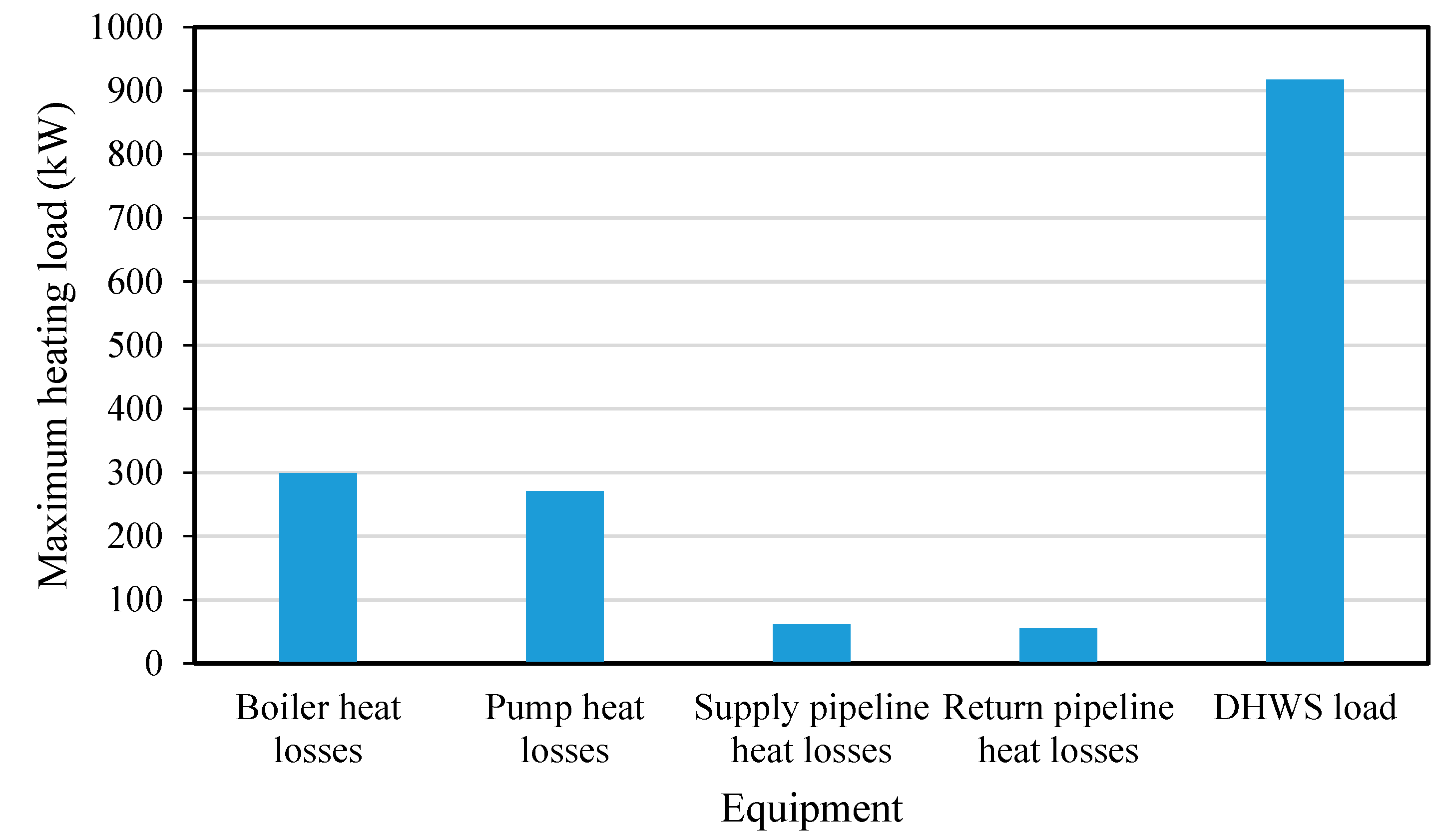
The heat losses from the boiler, pumps, supply and return pipelines, and DHWS are obtained using Equations (10)–(26). Figure 15 presents the chart of heat losses in which the deviations for the years are negligible.

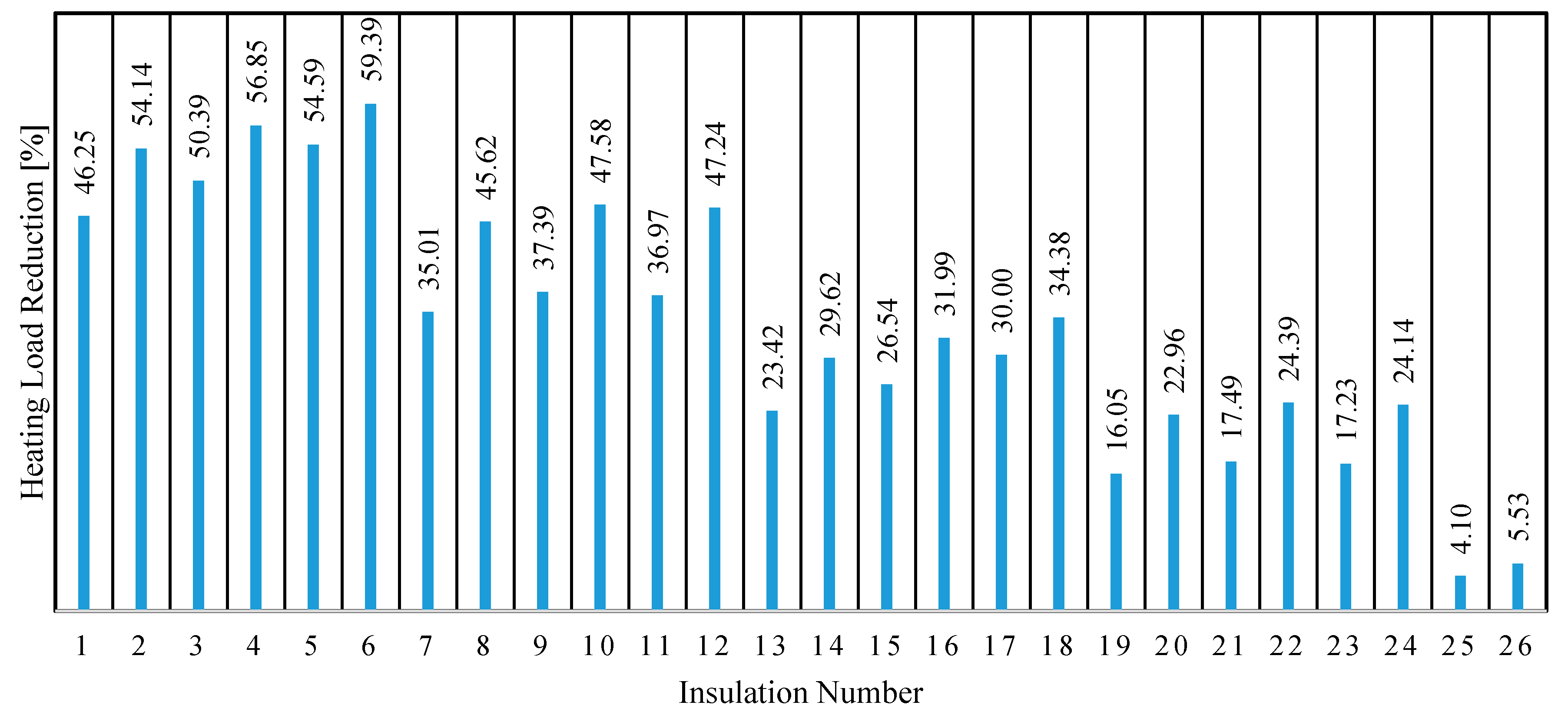
The desired heating load reductions for each retrofitted residential building scenario are presented in Figure 16. When all the exterior walls are insulated by the insulation case number 6, the heating load shows a 59% reduction. When only the ceiling is insulated with the same material (case number 18), the amount of load reduction is 34%. By replacing the windows from single-layer to double- and triple-layers for the insulation case number 25 and 26, the heat load reduction changes are only 4 and 5.5%, respectively.

5.3. Environmental Impacts

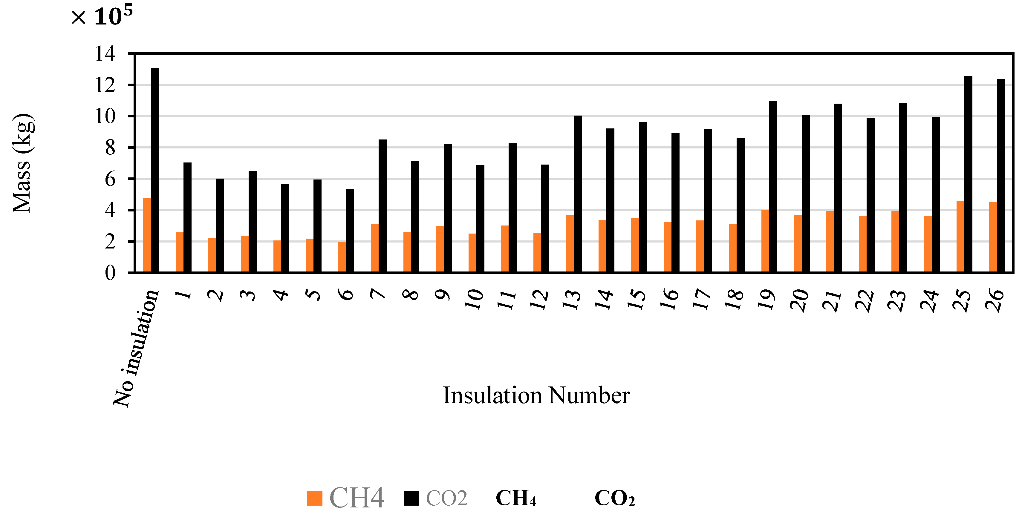
From the total annual heating demand for the different insulation scenarios and by use of the data presented in Table 6, the annual CO₂ emission and natural gas consumption are calculated. According to Figure 17, when the buildings are not insulated, the annual amount of CO₂ emission is 1308 tons, and the gas consumption is 475 tons. Least CO₂ emission belongs to polyurethane with 10 cm thickness. When all of the exterior walls are insulated perfectly, the annual amount of CO₂ emission and gas consumption is calculated as 531 and 193 tons, respectively.

5.4. Economic Analysis

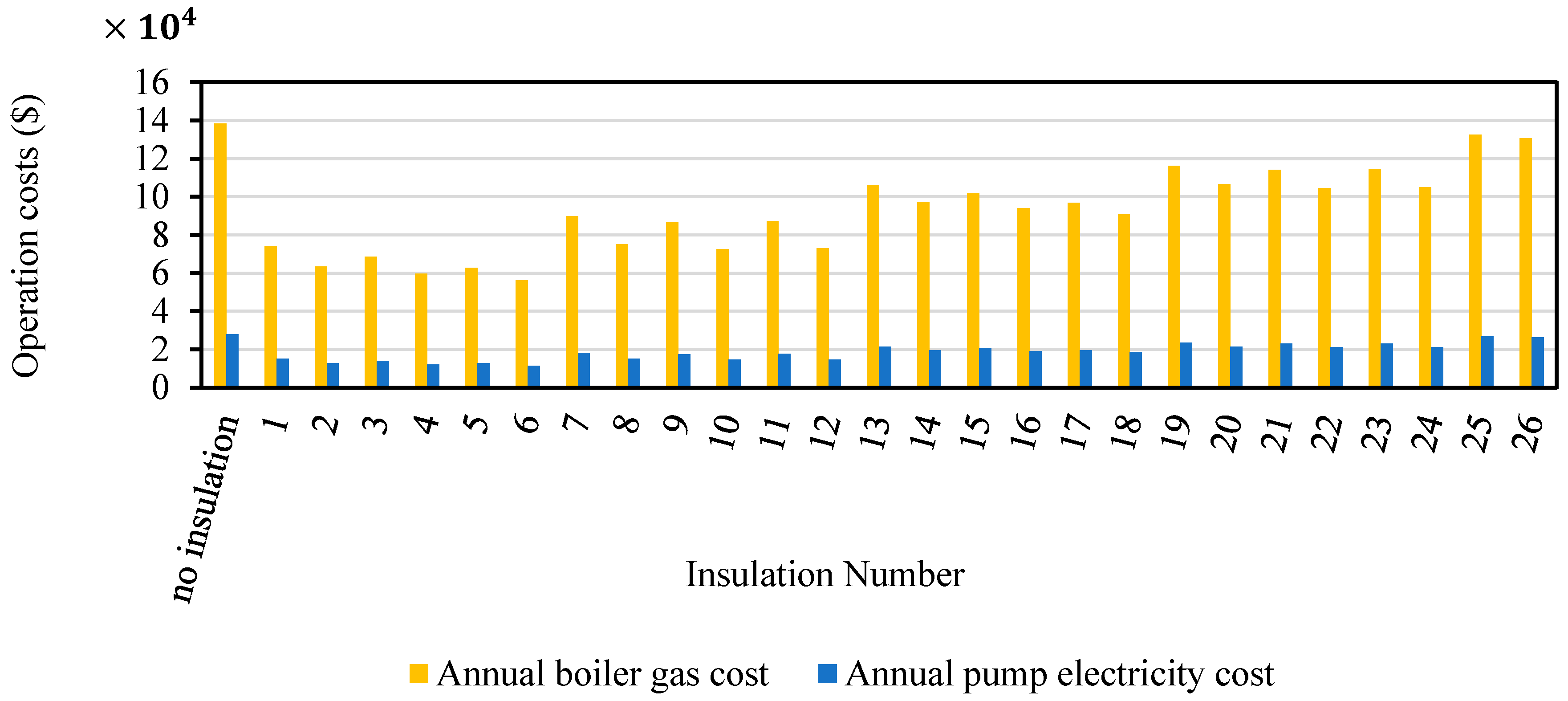
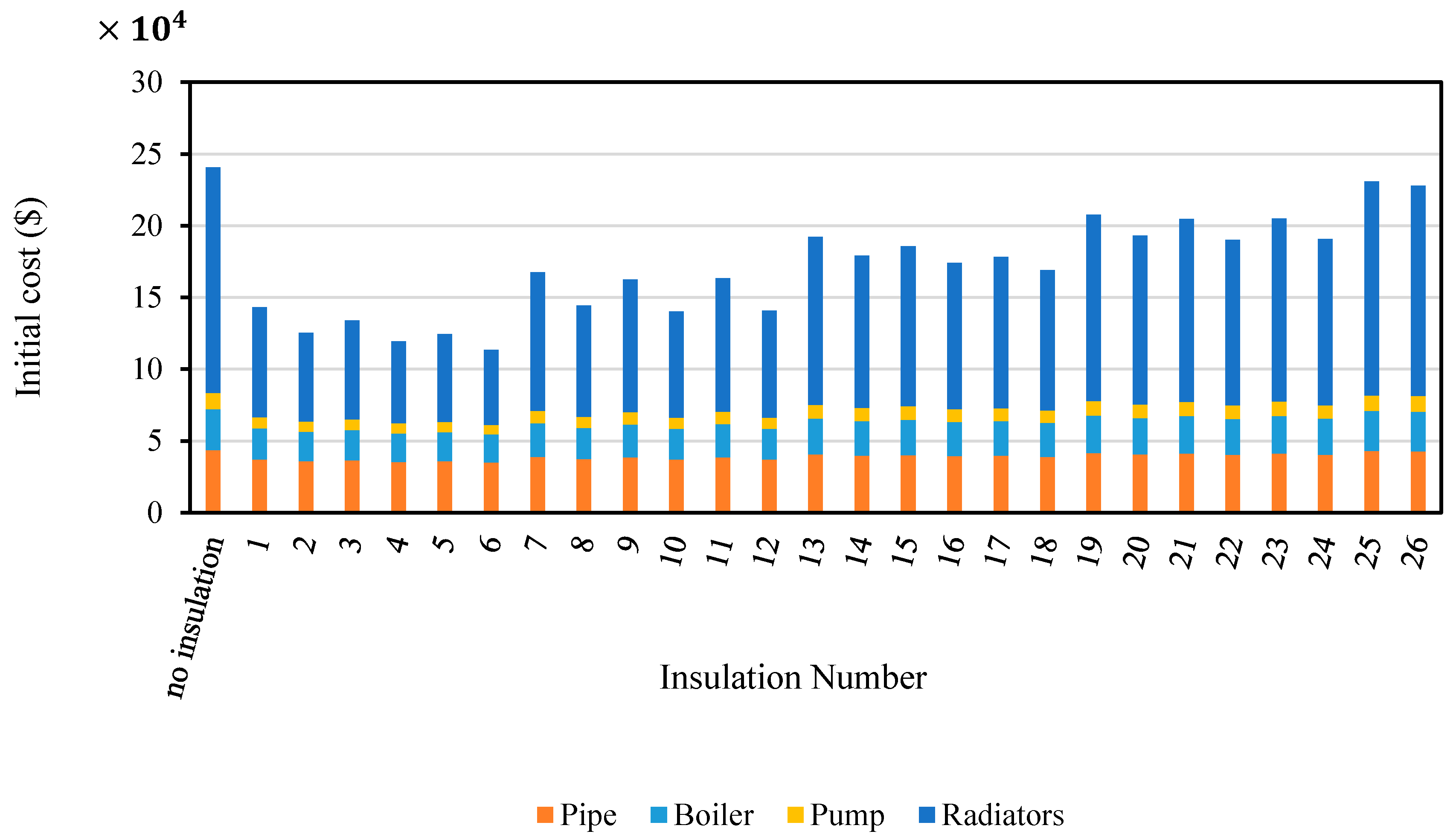
Because Qinarjeh is located in high altitude mountains, gas piping conducted by the government is not profitable. Therefore, in cost calculations, in addition to the cost of gas, the cost of transportation is also calculated, which is accounted as 0.21 $ per cubic meter of gas. Also, the electricity cost for the power of pumps is considered as 0.05 $/kWh. Figure 18 shows the annual gas and electricity price for different insulation scenarios. For the existing buildings, the annual cost of gas and electricity price are estimated to be 138,284 $ and 27,878 $, respectively. When all the exterior walls are insulated perfectly with a polyurethane layer of 10 cm thickness, the annual cost of gas and electricity price are estimated to be 56,151 and 11,320 $, respectively. Changes in the equipment cost by selecting different insulation scenarios are presented in Figure 19, which indicates that the most mutant equipment is radiators. This means that by choosing the best insulation for the building, the size of radiators and subsequently the costs of that can be reduced incrementally. For the existing buildings and the insulation case number 6, the total radiators costs and electricity are estimated to be 157,247 and 52,179 $, respectively.

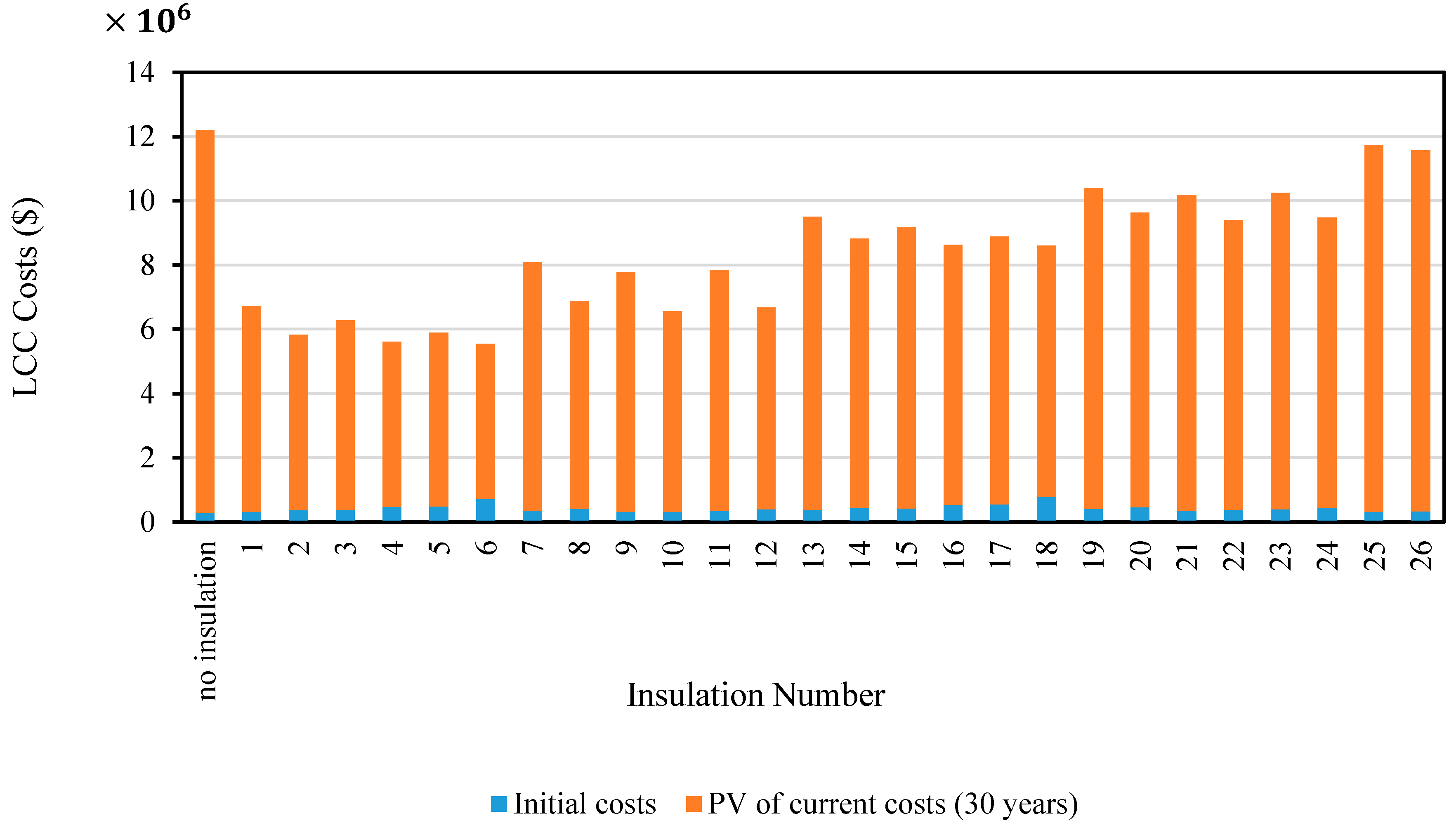
After calculating the total initial and operation costs using Equations (29)–(32), the LCC for the 30-year periods is estimated as illustrated in Figure 20. Initial costs and the LCC for the existing building with no insulation are estimated to be 295,339 $ and 12,197,615 $, respectively. Glass wool has the minimum initial cost according to the insulation layers (315,055 $), with the properties of case number nine reported in Table 5. The minimum LCC belongs to the polyurethane insulation layer with the properties of case number 6, which is accounted as 5,546,702 $.

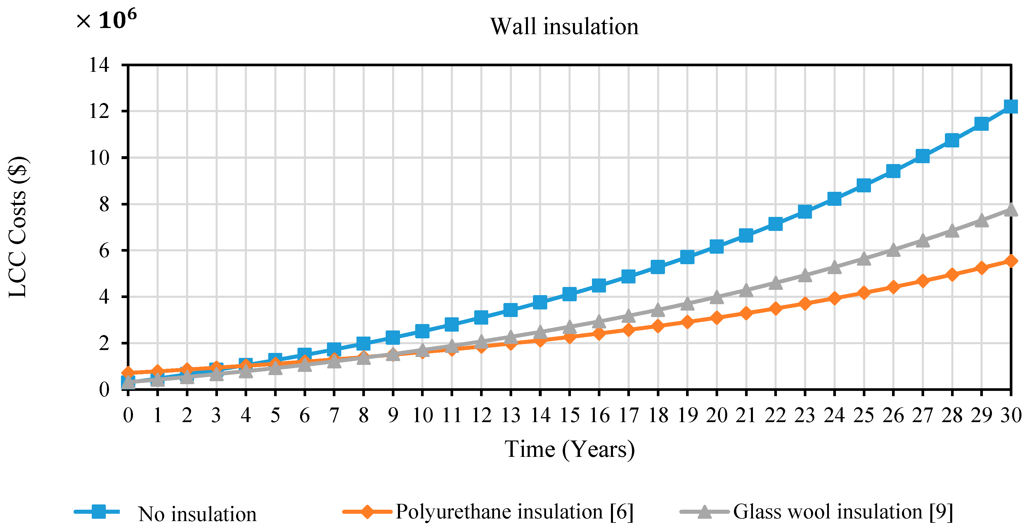
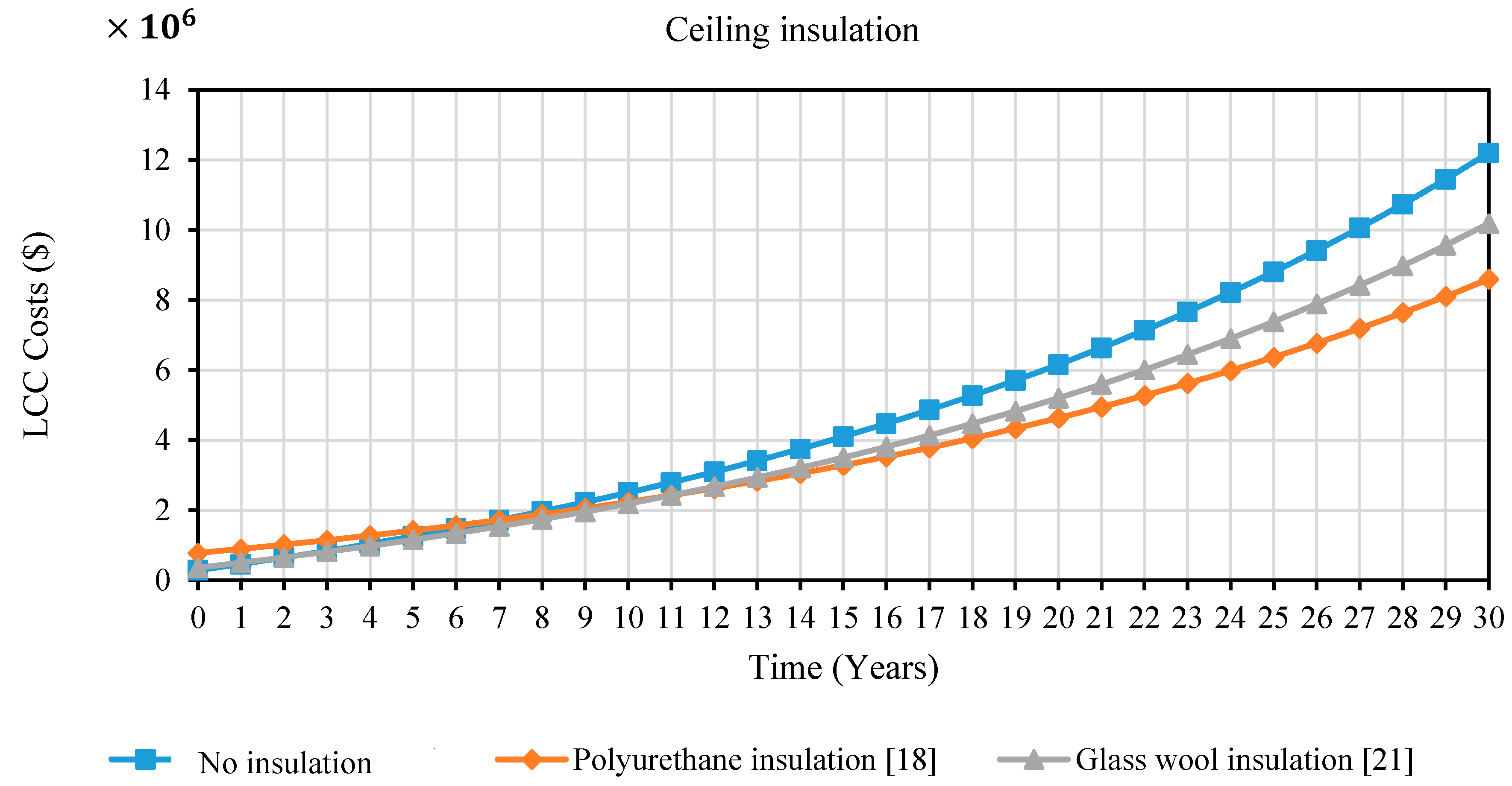
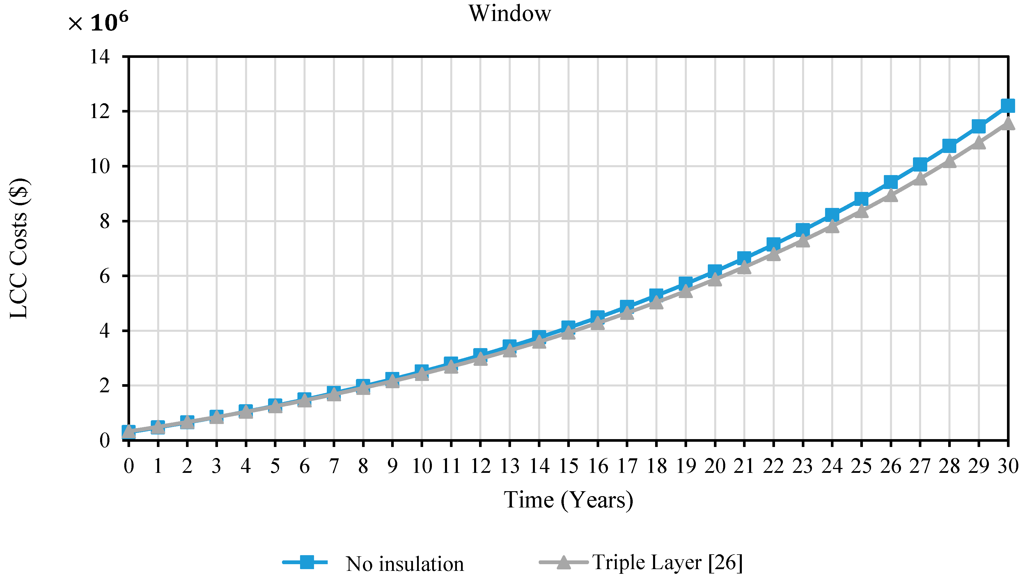
Cost behavior of different life cycle periods for the most critical insulation scenarios is presented in Figure 21, Figure 22 and Figure 23. In these figures, the time zero corresponds to the initial costs and the payback period will be obtained at a point where no insulation curves crossing the insulation curves. The maximum payback period is seven years, which belongs to the insulation of the ceiling with a polyurethane layer of 10 cm thickness. Moreover, the payback for the same materials is four years when all the exterior walls are insulated. The minimum payback period is one year, which belongs to the glass wool with the properties of case number 9 reported in Table 5. In addition, the payback period by retrofitting of the windows with triple layers is three years.

5.5. General System Optimization

For the general optimization, the type of insulation for the buildings and the pipes are selected as the polyurethane and the elastomeric type, respectively. This selection is due to its properties in saving the costs. The target function is defined as minimizing the LCC, which is considered for 30 years. For the general DH system optimization, unlike Section 5.4, the costs of pipes and elastomeric insulation for DHWS and excavation are considered as the initial costs in Equation (30). The excavation cost is assumed to be 1.875 $ per each cubic meter volume. The results of the optimization are presented in

Table 9. Comparison between the initial and the optimized values of the studied variables.

Variable	Initial Value (No Optimization)	Optimized Value (with Considering Climate Change)
Ceiling insulation thickness	0 (m)	0.128 (m)
Wall insulation thickness	0 (m)	0.140 (m)
Depth of buried heating supply pipes	1 (m)	3.494 (m)
Depth of DHWS pipes	1 (m)	1.052 (m)
Pipe insulation thickness	0.01 (m)	0.031 (m)
Outlet boiler Temperature	82 (°C)	91.14 (°C)

. In the first column of values, the climate change impact is not considered, and in the second one, the impact of climate changes has been applied.

For investigating the effects of the climate changes on the calculated data, the optimized results with PSO method has been compared with the initial results in

Table 10. Comparison of economic and environmental parameters.

	Without Considering Climate Changes		Considering Climate Changes
	No Optimization	PSO Optimization	No Optimization	PSO Optimization
LCC ($) (30years)	$2.48\times {10}^7$	$1.65\times {10}^7$	$2.15\times {10}^7$	$1.61\times {10}^7$
Initial cost ($)	$4.54\times {10}^5$	$1.01\times {10}^7$	$4.65\times {10}^5$	1.01 $\times {10}^7$
Gas cost ($) (30 years)	2.10 $\times {10}^7$	6.07 $\times {10}^6$	1.83 $\times {10}^7$	5.75 $\times {10}^6$
Electricity cost ($) (30 years)	3.30 $\times {10}^6$	3.48 $\times {10}^5$	2.75 $\times {10}^6$	2.83 $\times {10}^5$
Total heating load (kwh/30years)	4.62 $\times {10}^8$	1.33 $\times {10}^8$	4.07 $\times {10}^8$	1.27 $\times {10}^8$
Pumps powers (kwh/30years)	2.77 $\times {10}^7$	2.91 $\times {10}^6$	2.34 $\times {10}^7$	2.42 $\times {10}^6$
CH4 (kg/30 years)	3.03 $\times {10}^7$	8.75 $\times {10}^6$	2.67 $\times {10}^7$	8.33 $\times {10}^6$
CO2 (kg/30 years)	8.33 $\times {10}^7$	2.41 $\times {10}^6$	7.34 $\times {10}^7$	2.29 $\times {10}^7$

In this table all economic and environmental parameters for the general optimization have been compared between the data extracted from PSO method and the initial results. It has been observed that by considering the climate change effects in a period of 30 years, the optimized and nonoptimized values show a reducing trend. On the other hand, the initial costs remained unchanged, meaning that climate changes are not affecting the initial investments.

6. Conclusions

In this research work, an optimized approach to save energy has been adopted by investigating the application of different types of insulation materials for residential buildings. Qinarjeh village, which is in the north-west of Iran, is selected in this case study. In order to design the efficient buildings, these units are connected through a DH system with the perspective of the future demands regarding climate changes, environmental impacts, and economical concerns. The obtained results show that how climate changes and different types of insulations can influence heating demands, costs, and air pollution. The main concluding results are listed in the following points.

• When all the exterior walls are insulated, only a good insulation material with high resistance, like polyurethane, can reduce heating demand by 59%.
• When a cost investment limitation for the insulation of all the building sides is a matter of concern, the heating demand reduction, by adopting the insulating layers at the exterior walls are a better choice compared to the ceiling.
• Climate changes can cause a reduction in heating demands and CO₂ emission up to 20% until the 2040s because of the trend of global warming.
• Insulating the building sides in a DH network can cause significant effects on the initial and operating costs including the gas consumption and radiators sizes. For this specific case, the payback period of the insulating building investment is between one to seven years.
• Glass wool is the best choice from the payback period efficiency point of view because the investment cost can be compensated after one year.
• According to the results, polyurethane could be the best choice for the environment if the investment cost is not an issue and the optimal thickness suggestion is 14 cm.
• For a minimal investment, glass wool could be a good choice.
• Both high and low degrees of the outlet temperature of the boiler have their own benefits. The high temperature of the supply water causes the size of heating equipment like radiators to decrease while low-temperature decreases the pipes heat losses to the surrounding.
• The optimal suggestion outlet temperature of the boiler in a DH system is between 90 and 95 °C.
• The minimum optimal depth of buried pipes, from the point of view of costs and fewer heat losses, is between 1.5 and 3 m underground and for the elastomeric insulation choice; the optimal thickness suggestion is 2 cm.

Therefore, in cold mountains, climate classification of Iran, retrofitting the building envelope can reduce the energy consumption of the DH system up to 60%.

It is noteworthy to mention that, for the energy saving and environmental benefits, it is important that civil engineers pay more attention to the different types of insulation material in the first step of their design of the energy efficient buildings. Polyurethane could be the best insulation because of high thermal resistance and different available forms such as solid and spray in the market. On the other hand, this insulation material still has a high price and a lengthy payback investment period. In this work, by using an optimized DH system, which considers the climate changes, a reduction of air pollution could be possible. As a result of such application, the payback period of the investment costs for the expensive insulation material will be decreased according to the defined conditions. The future study could be dedicated to optimizing the different parameters of the DH systems in a cooling mode by considering future weather projection.

References

- Rezaie, B.; Rosen, M.A. District heating and cooling: Review of technology and potential enhancements. Appl. Energy 2012, 93, 2–10. [Google Scholar] [CrossRef]
- Lund, H.; Möller, B.; Mathiesen, B.V.; Dyrelund, A. The role of district heating in future renewable energy systems. Energy 2010, 35, 1381–1390. [Google Scholar] [CrossRef]
- Phetteplace, G.; Bahnfleth, D.; Mildenstein, P.; Overgaard, J.; Rafferty, K.; Wade, D. District Heating Guide; ASHRAE: Atlanta, GA, USA, 2013. [Google Scholar]
- Dotzauer, E. Simple model for prediction of loads in district-heating systems. Appl. Energy 2002, 73, 277–284. [Google Scholar] [CrossRef]
- Doračić, B.; Novosel, T.; Pukšec, T.; Duić, N. Evaluation of Excess Heat Utilization in District Heating Systems by Implementing Levelized Cost of Excess Heat. Energies 2018, 11, 575. [Google Scholar]
- Sáez Blázquez, C.; Farfán Martín, A.; Nieto, I.; González-Aguilera, D. Economic and Environmental Analysis of Different District Heating Systems Aided by Geothermal Energy. Energies 2018, 11, 1265. [Google Scholar] [Green Version]
- Biserni, C.; Valdiserri, P.; D’Orazio, D.; Garai, M. Energy Retrofitting Strategies and Economic Assessments: The Case Study of a Residential Complex Using Utility Bills. Energies 2018, 11, 2055. [Google Scholar] [CrossRef]
- Schlueter, A.; Thesseling, F. Building information model based energy/exergy performance assessment in early design stages. Autom. Constr. 2009, 18, 153–163. [Google Scholar] [CrossRef]
- Rosa, D.A.; Christensen, J.E. Low-energy district heating in energy-efficient building areas. Energy 2011, 36, 6890–6899. [Google Scholar] [CrossRef] [Green Version]
- Keçebaş, A.; Alkan, M.A.; Bayhan, M. Thermo-economic analysis of pipe insulation for district heating piping systems. Appl. Therm. Eng. 2011, 31, 3929–3937. [Google Scholar]
- Haichao, W.; Wenling, J.; Lahdelma, R.; Pinghua, Z.; Shuhui, Z. Atmospheric environmental impact assessment of a combined district heating system. Build. Environ. 2013, 64, 200–212. [Google Scholar] [CrossRef]
- Pirouti, M.; Bagdanavicius, A.; Ekanayake, J.; Wu, J.; Jenkins, N. Energy consumption and economic analyses of a district heating network. Energy 2013, 57, 149–159. [Google Scholar] [CrossRef]
- Torio, H.; Schmidt, D. Development of system concepts for improving the performance of a waste heat district heating network with exergy analysis. Energy Build. 2010, 42, 1601–1609. [Google Scholar] [CrossRef]
- Ahn, J.; Cho, S. Development of an intelligent building controller to mitigate indoor thermal dissatisfaction and peak energy demands in a district heating system. Build. Environ. 2017, 124, 57–68. [Google Scholar] [CrossRef]
- Lund, H.; Werner, S.; Wiltshire, R.; Svendsen, S.; Thorsen, J.E.; Hvelplund, F.; Mathiesen, B.V. 4th Generation District Heating (4GDH): Integrating smart thermal grids into future sustainable energy systems. Energy 2014, 68, 1–11. [Google Scholar] [CrossRef]
- Tańczuk, M.; Masiukiewicz, M.; Anweiler, S.; Junga, R. Technical Aspects and Energy Effects of Waste Heat Recovery from District Heating Boiler Slag. Energies 2018, 11, 796. [Google Scholar] [CrossRef]
- Vesterlund, M.; Toffolo, A. Design Optimization of a District Heating Network Expansion, a Case Study for the Town of Kiruna. Appl. Sci. 2017, 7, 488. [Google Scholar] [CrossRef]
- IPCC. Climate Change 2007: The Physical Science Basis; Cambridge University Press: Cambridge, UK, 2007; p. 996. [Google Scholar]
- Daaboul, J.; Ghali, K.; Ghaddar, N. Mixed-mode ventilation and air conditioning as alternative for energy savings: a case study in Beirut current and future climate. Energy Effic. 2018, 11, 13–30. [Google Scholar] [CrossRef]
- Torio, H.; Schmidt, D.; Ecbcs, A. 49—Low Exergy Systems for High Performance Buildings and Communities (Annex 49 Final Report); Fraunhofer IBP/IEA: München, Germany, 2011. [Google Scholar]
- Picallo-Perez, A.; Sala-Lizarraga, J.M.; Iribar-Solabarrieta, E.; Hidalgo-Betanzos, J.M. A symbolic exergoeconomic study of a retrofitted heating and DHW facility. Sustain. Energy Technol. Assess. 2018, 27, 119–133. [Google Scholar] [CrossRef]
- Bell, A.A.; Angel, W.L. HVAC Equations, Data, and Rules of Thumb; McGraw-Hill: New York, NY, USA, 2000. [Google Scholar]
- Ashrae, F. Fundamentals Handbook. Available online: https://www.ashrae.org/technical-resources/ashrae-handbook/description-2017-ashrae-handbook-fundamentals (accessed on 14 February 2019).
- Sonntag, R.E.; Borgnakke, C.; Van Wylen, G.J.; Van Wyk, S. Fundamentals of Thermodynamics; Wiley: New York, NY, USA, 1998; Volume 6. [Google Scholar]
- Gülich, J.F. Centrifugal Pumps; Springer: Berlin, Germany, 2008; Volume 2, Available online: https://link.springer.com/book/10.1007%2F978-3-540-73695-0 (accessed on 14 February 2019).
- Tittelein, P.; Achard, G.; Wurtz, E. Modelling earth-to-air heat exchanger behaviour with the convolutive response factors method. Appl. Energy 2009, 86, 1683–1691. [Google Scholar] [CrossRef]
- Habibi, M.; Hakkaki-Fard, A. Evaluation and improvement of the thermal performance of different types of horizontal ground heat exchangers based on techno-economic analysis. Energy Convers. Manag. 2018, 171, 1177–1192. [Google Scholar] [CrossRef]
- Bejan, A. Convection Heat Transfer; John Wiley & Sons: Hoboken, NJ, USA, 2013; Available online: https://www.wiley.com/en-ir/Convection+Heat+Transfer%2C+4th+Edition-p-9781118330081 (accessed on 14 February 2019).
- Holman, J. Heat Transfer, 9th ed. Available online: https://aiche.onlinelibrary.wiley.com/doi/10.1002/aic.690230338 (accessed on 14 February 2019).
- Giardina, J.J. Evaluation of Ground Coupled Heat Pumps for the State of Wisconsin; University of Wisconsin--Madison: Madison, WI, USA, 1995. [Google Scholar]
- ASPE. Domestic Water Heating Design Manual, Amercian Society of Plumbing Engineers. 2003. Available online: https://www.aspe.org/content/domestic-water-heating-design-manual-2nd-edition-electronic-download (accessed on 14 February 2019).
- Goldner, F. Energy Use and Domestic Hot Water Consumption-Phase 1. Final Report; New York State Energy Research and Development Authority: New York, NY, USA; Energy Management and Research Associates: Brooklyn, NY, USA, 1994.
- Yang, X.; Tysoe, B. Disparate standards: comparing standard domestic hot water modeling methods for multi-resdential buildings. Available online: http://ibpsa-usa.org/index.php/ibpusa/article/download/351/337 (accessed on 14 February 2019).
- Weil, L.R.; Schipper, K.; Francis, J. Financial Accounting: An Introduction to Concepts, Methods and Uses; Cengage Learning: Boston, MA, USA, 2013; Available online: https://www.cengagebrain.co.uk/shop/isbn/9781111823450?parent_category_rn=&top_category=&urlLangId=1&errorViewName=ProductDisplayErrorView&categoryId=&urlRequestType=Base&partNumber=9781111823450&cid=GB1 (accessed on 14 February 2019).
- Hakkaki-Fard, A.; Eslami-Nejad, P.; Aidoun, Z.; Ouzzane, M. A techno-economic comparison of a direct expansion ground-source and an air-source heat pump system in Canadian cold climates. Energy 2015, 87, 49–59. [Google Scholar] [CrossRef]
- Bradbury, J.; Clement, Z.; Down, A. Greenhouse Gas Emissions and Fuel Use within the Natural Gas Supply Chain–Sankey Diagram Methodology; Tech. Rep; Quadrennial Energy Review Analysis; Department of Energy, Office of Energy Policy and Systems Analysis: Washington, DC, USA, 2015. Available online: https://www.energy.gov/ (accessed on 14 February 2019).
- Lim, Y.S.; Montakhab, M.; Nouri, H. A Constriction Factor Based Particle Swarm Optimization for Economic Dispatch. 2009. Available online: http://eprints.uwe.ac.uk/13171/1/PSO_Final_Sept23.pdf (accessed on 14 February 2019).
- Clerc, M. The swarm and the queen: towards a deterministic and adaptive particle swarm optimization. In Evolutionary Computation 1999, CEC 99, Proceedings of the 1999 Congress on; IEEE: Piscataway, NJ, USA, 1999; Available online: https://ieeexplore.ieee.org/abstract/document/785513 (accessed on 14 February 2019). [CrossRef]
- Almeida, P.; Carvalho, M.J.; Amorim, R.; Mendes, J.F.; Lopes, V. Dynamic testing of systems–Use of TRNSYS as an approach for parameter identification. Sol. Energy 2014, 104, 60–70. [Google Scholar] [CrossRef]
- Wetter, M. GenOpt (R), Generic Optimization Program, User Manual, Version 2.0.0. 2003. Available online: https://cloudfront.escholarship.org/dist/prd/content/qt5dp8q7m1/qt5dp8q7m1.pdf (accessed on 14 February 2019).
Figure 1.
Classification of Iran climate map.
Figure 2.
The satellite view of the center of Qinarjeh village (Google Maps 2019, Retrieved 13 February 2019).
Figure 3.
Hourly and monthly average ambient temperature of Qinarjeh village for years between 2000 and 2010.
Figure 4.
Monthly average RH and total radiation for the years between 2000 and 2010.
Figure 5.
Future ambient temperature projection of Qinarjeh village for (a) year 2020; (b) year 2030; (c) year 2040; and (d) future average monthly ambient temperature projection of Qinarjeh village until the 2050 s.
Figure 6.
(a) Sample of old building of the village; (b) temperature contour of the building recorded at 30/10/2018, 8:00AM; (c) a sample model of building with the specified property in Table 1; and (d) top view of the sample building.
Figure 7.
Total area of the buildings in the village, which is calculated as 75,156 square meters.
Figure 8.
(a) Main pipeline location; (b) Plan of supply and return of main and sub-branches pipelines.
Figure 9.
Hourly hot water flow rate used profile for one person in one day.
Figure 10.
Schematic flowchart for evaluating different retrofit scenarios.
Figure 11.
Equipment prices: (a) boiler prices in dollar currency for different heating loads (kW); (b) price of elastomeric insulation for different thickness per square meter in dollar currency; (c) pipe prices for different diameters; and (d) pump prices for different powers (kW).
Figure 12.
Schematic flowchart of the Particle Swarm Optimization (PSO) optimization method.
Figure 13.
Hourly simulation of the heating load in different years diagrams: (a) Average of the heating load (kW) for the years between 2000 and 2010; (b) heating load (kW) in the year 2020; (c) heating load in the year 2030; and (d) heating load (kW) in the year 2030.
Figure 14.
Comparison of the amount of total annual heating demand for different insulation types based on Table 5 for different years.
Figure 15.
Bar chart of heat losses from the equipment [kW].
Figure 16.
Desired load reduction for different retrofitted residential buildings scenarios.
Figure 17.
Comparison of the annual CO2 emission and natural gas consumption for different insulation scenarios based on Table 5.
Figure 18.
Comparison of the annual gas and electricity cost for different insulation scenarios based on Table 5.
Figure 19.
Comparison of the initial equipment costs for different insulation scenarios based on Table 5.
Figure 20.
Comparison of the LCC for a 30-year period for different insulation scenarios based on Table 5.
Figure 21.
Comparison of the life cycle cost (LCC) for the insulation scenarios number 6 and 9 based on Table 5.
Figure 22.
Comparison of the LCC for the insulation scenarios number 18 and 21 based on Table 5.
Figure 23.
Comparison of the LCC for the windows with triple layer based on Table 5.