Efficient RES Penetration under Optimal Distributed Generation Placement Approach

 , , and
Abstract
:1. Introduction
2. Proposed Methodology
2.1. Problem Formulation
- , are the voltage magnitudes of bus i and j.
- is the conductance between buses i and j.
- , are the voltage angles of bus i and j.
- is the total number of branches.
- is the objective function.
- is the voltage of node i,
- , are the bus lower and upper voltage limits, respectively,
- is the current of k line, and,
- is the thermal current limit of k line.
- is the penalty function, or .
- is the objective function ().
- , are the penalty term and penalty factor, respectively.
- , refer to equality and inequality constraints, respectively.
- is the real power generation on bus i,
- is the reactive power generation on bus i,
- is the real power demand on bus i,
- is the reactive power demand on bus i,
- is the total number of network’s buses,
- is the total number of network’s lines,
- is the magnitude of bus admittance element ,
- is the angle of bus admittance element .
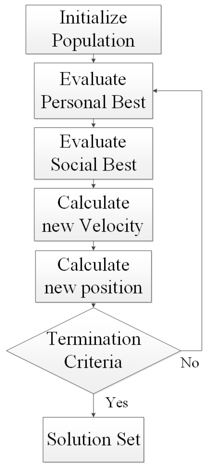
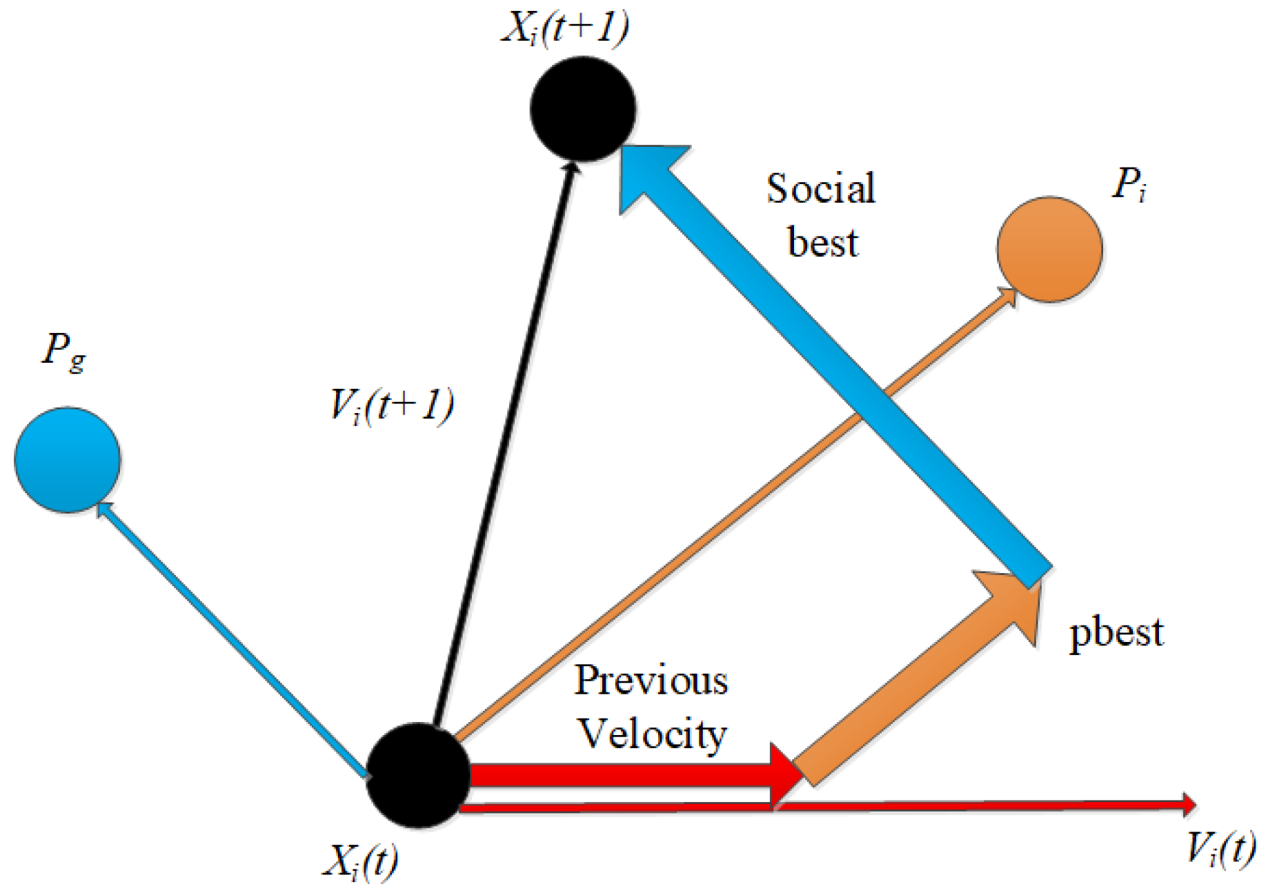
2.2. PSO for ODGP Problem
- i is the bus number.
- m the number of generators.
- refers to active power generation at ith node.
2.3. PSO for ORESP Problem
- is the number of RESs, and
- is the corresponding penalty term.
- optimal siting of RESs units,
- optimal sizing of RESs units,
- optimal aggregated RES capacity to be penetrated,
- optimal mix of RES technologies, and,
- optimal optimal number of units regarding each RES technology and in total,
3. Results
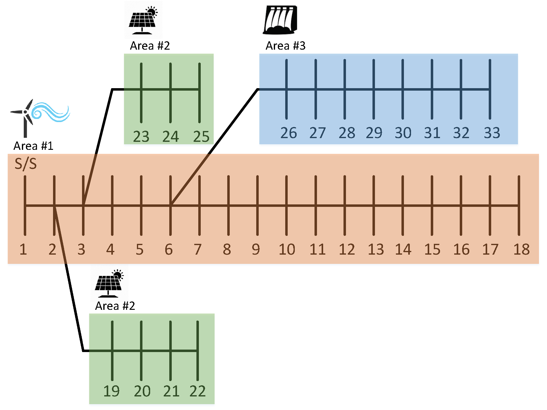
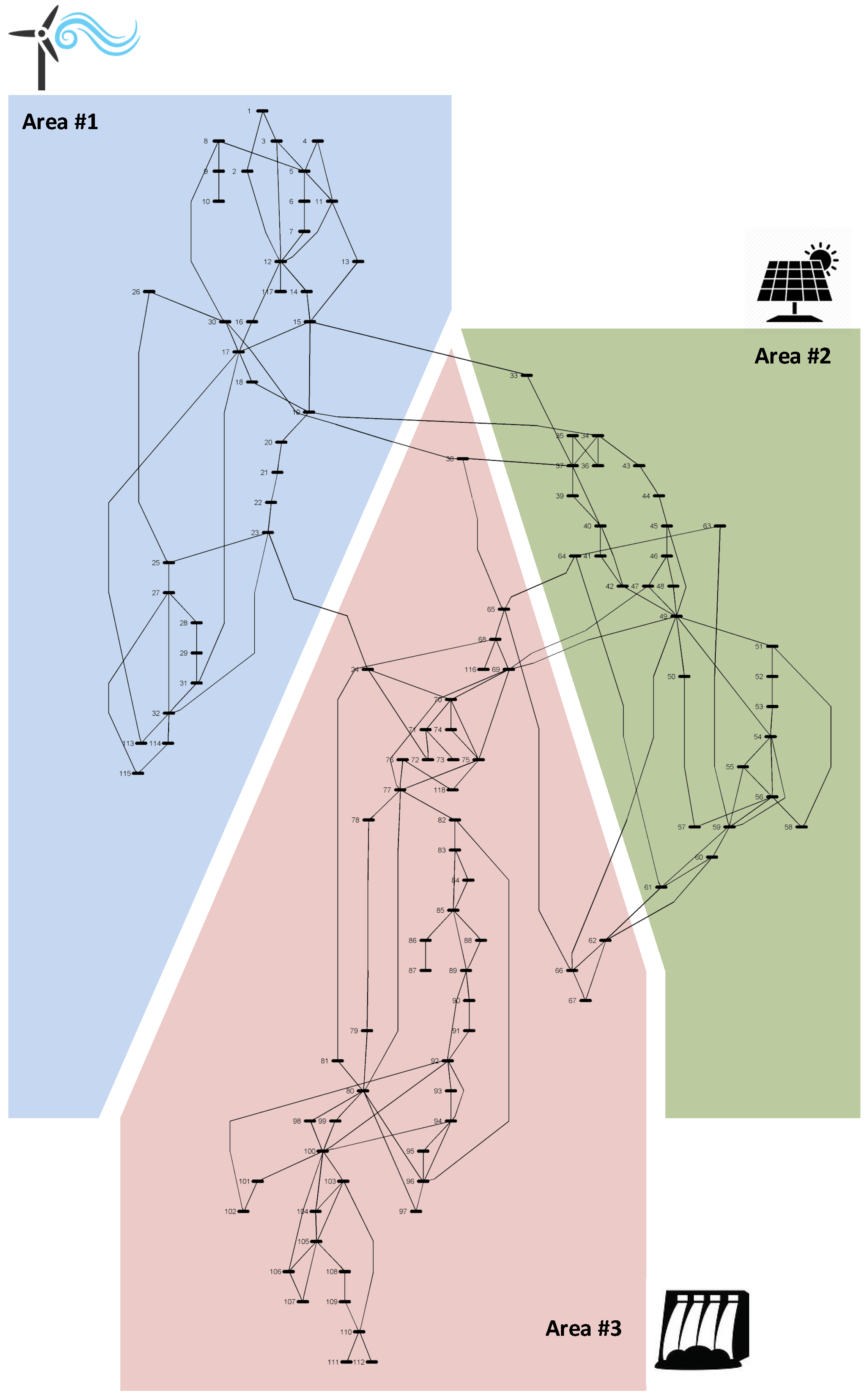
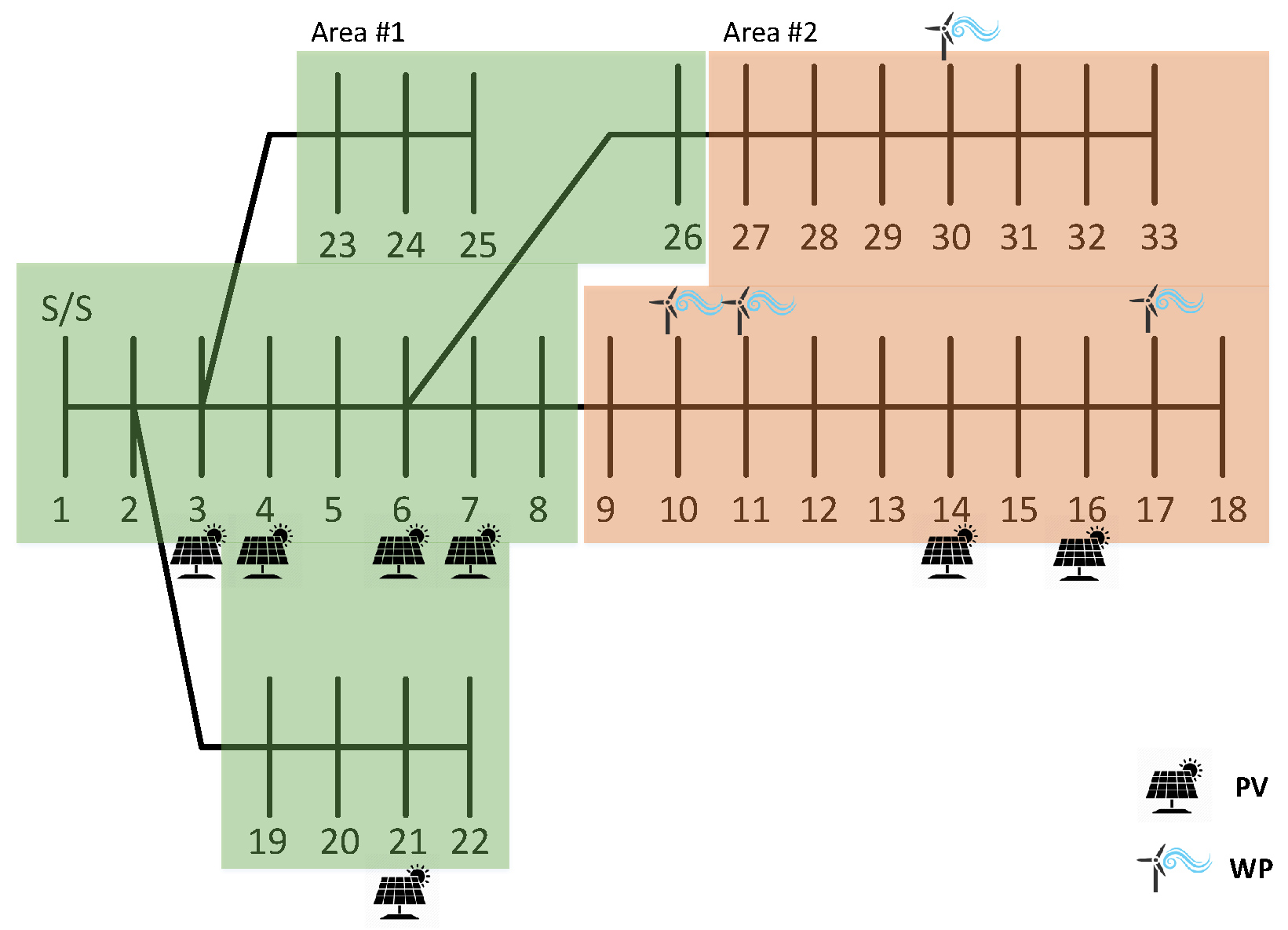
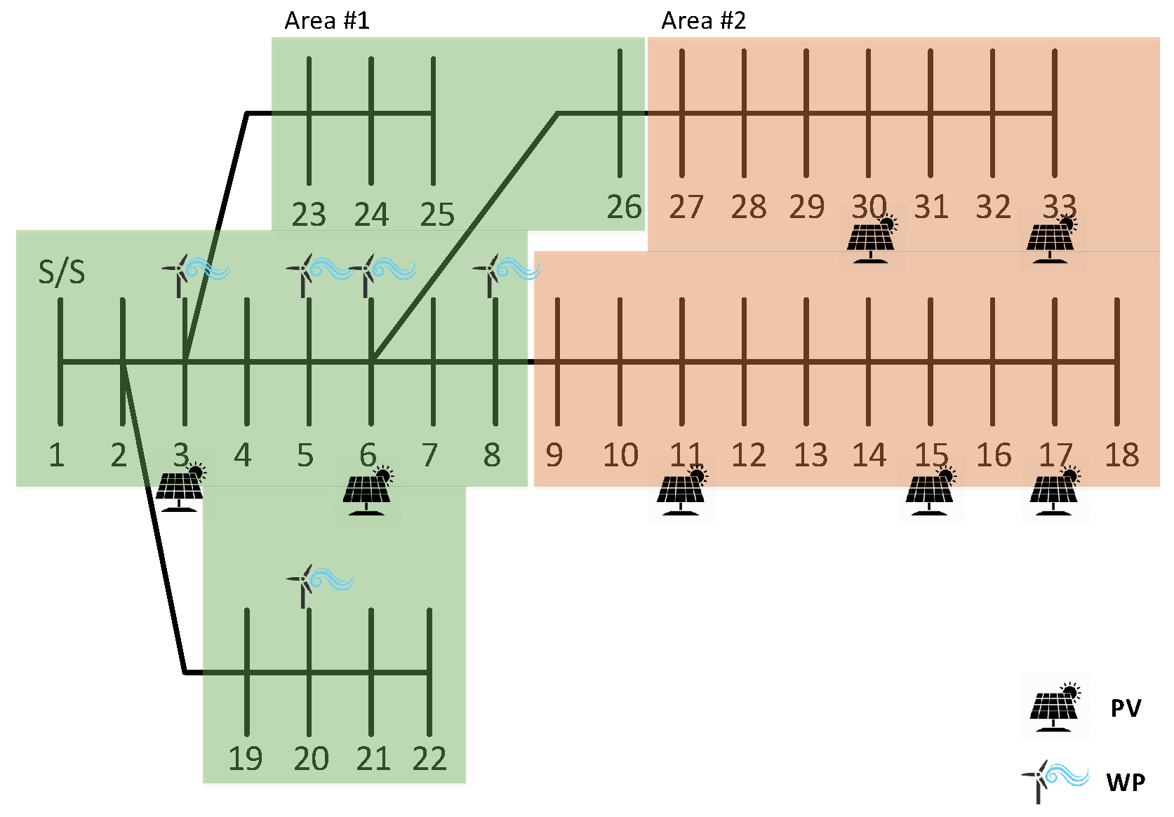
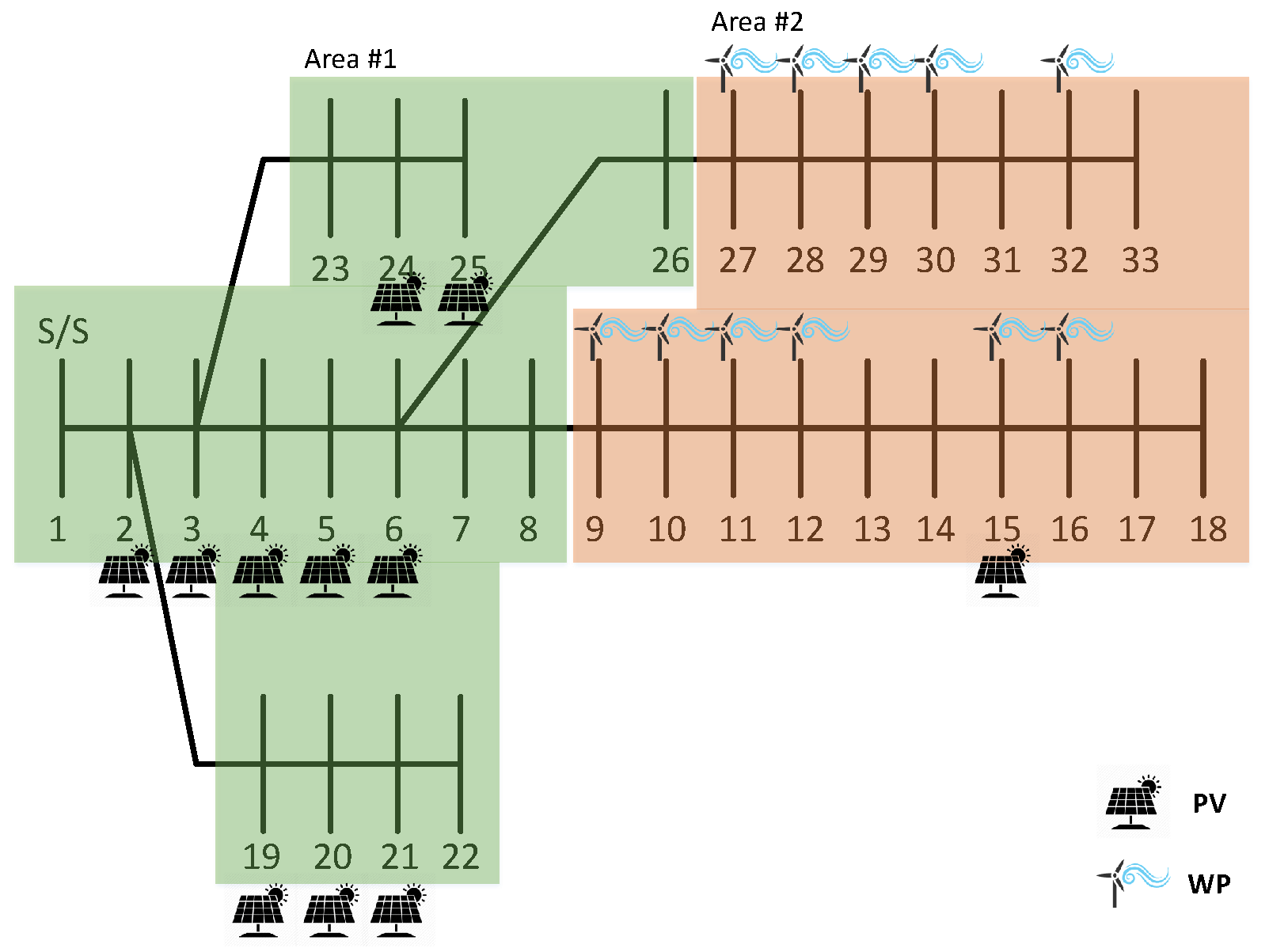
3.1. Examined DNs
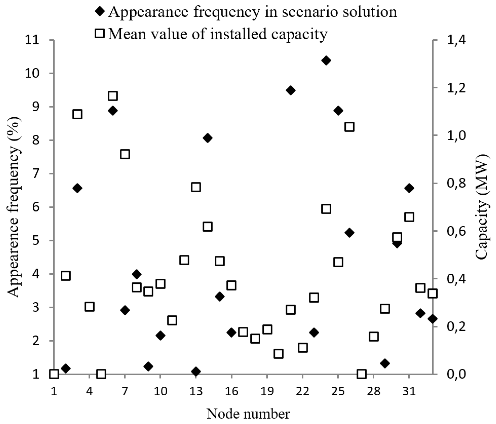
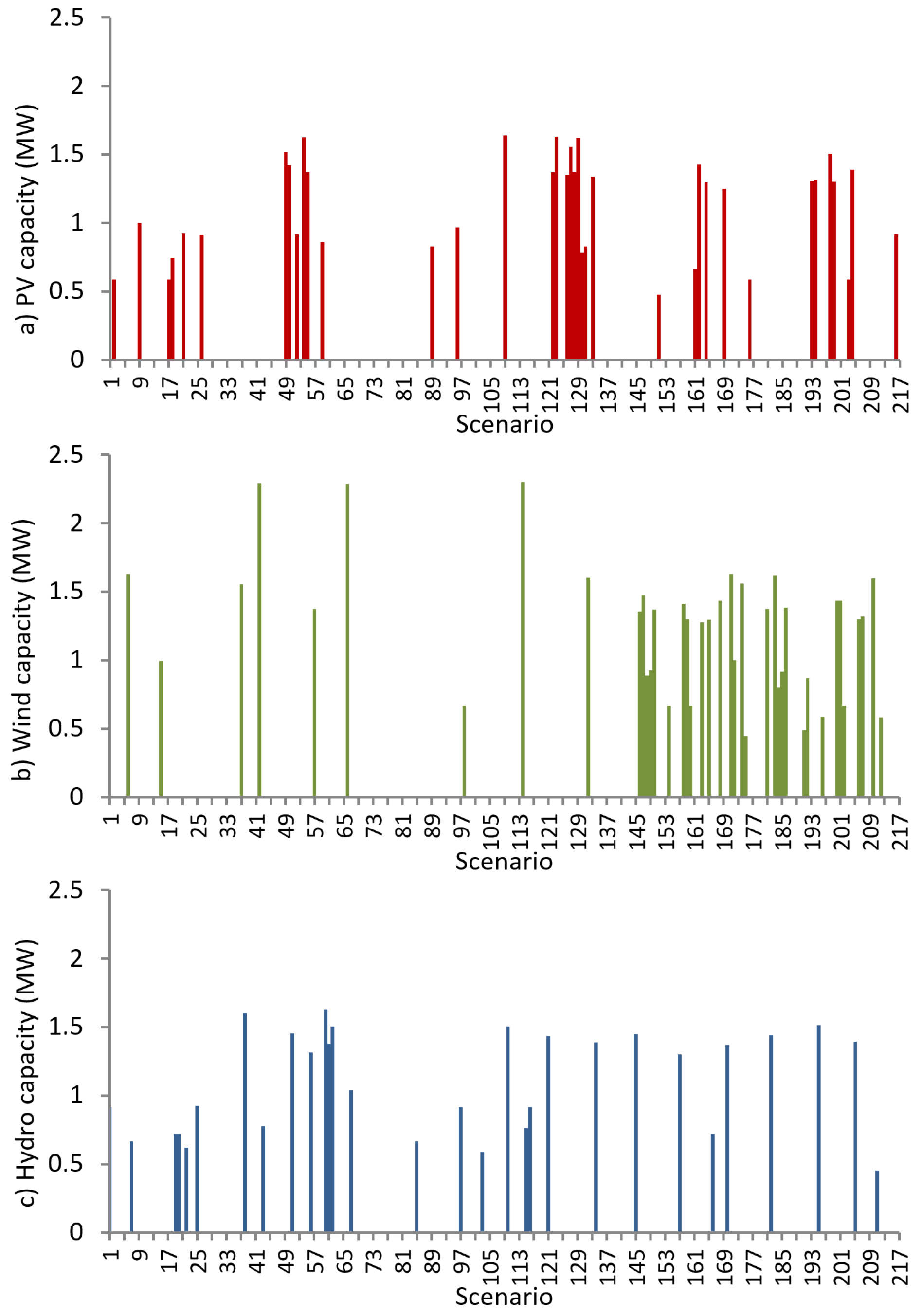
3.2. Results about the Examined Scenarios
3.3. Sensitivity Analysis Regarding the CFs Assignment
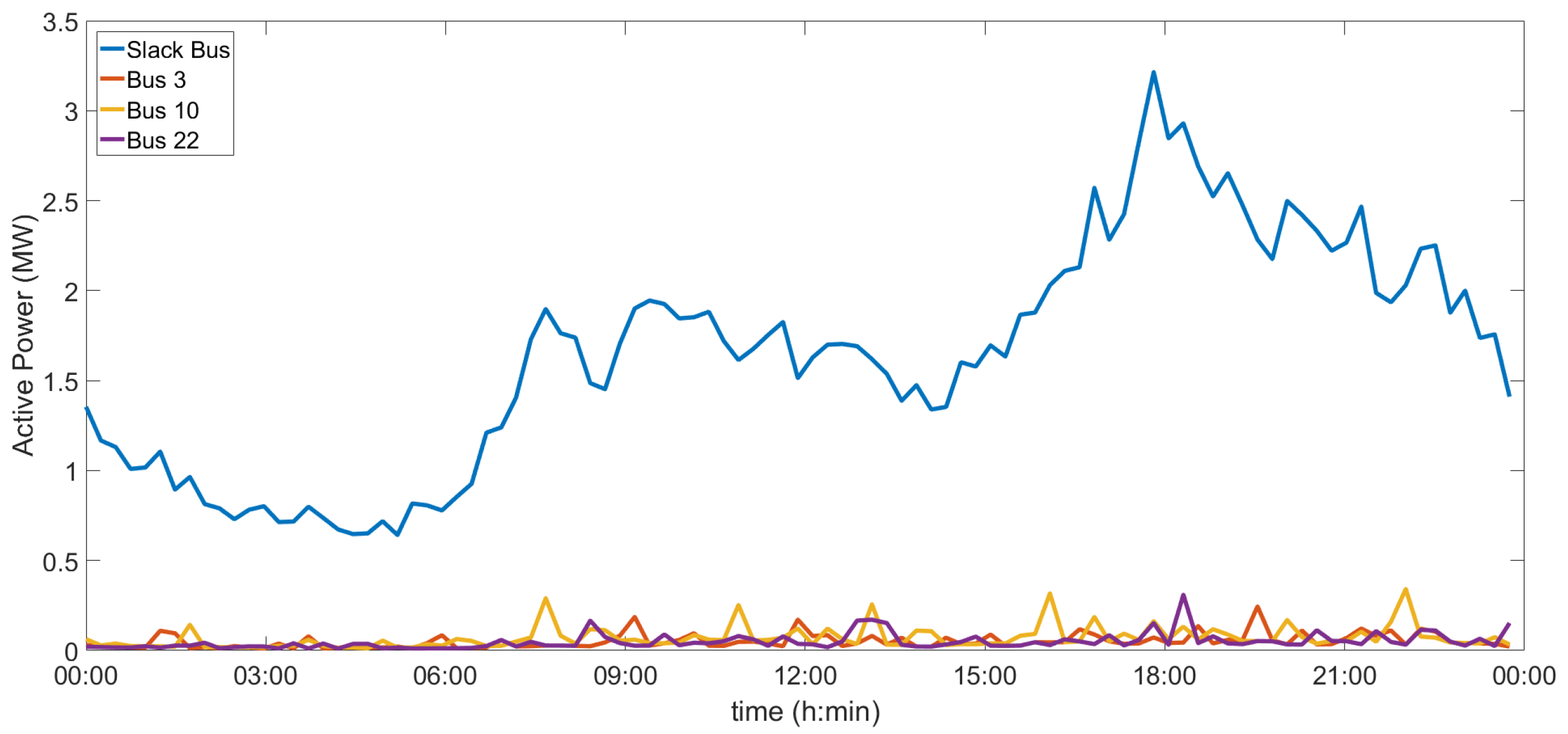
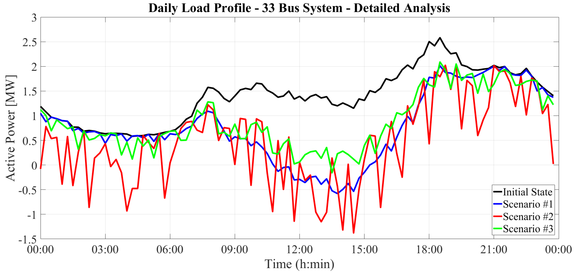
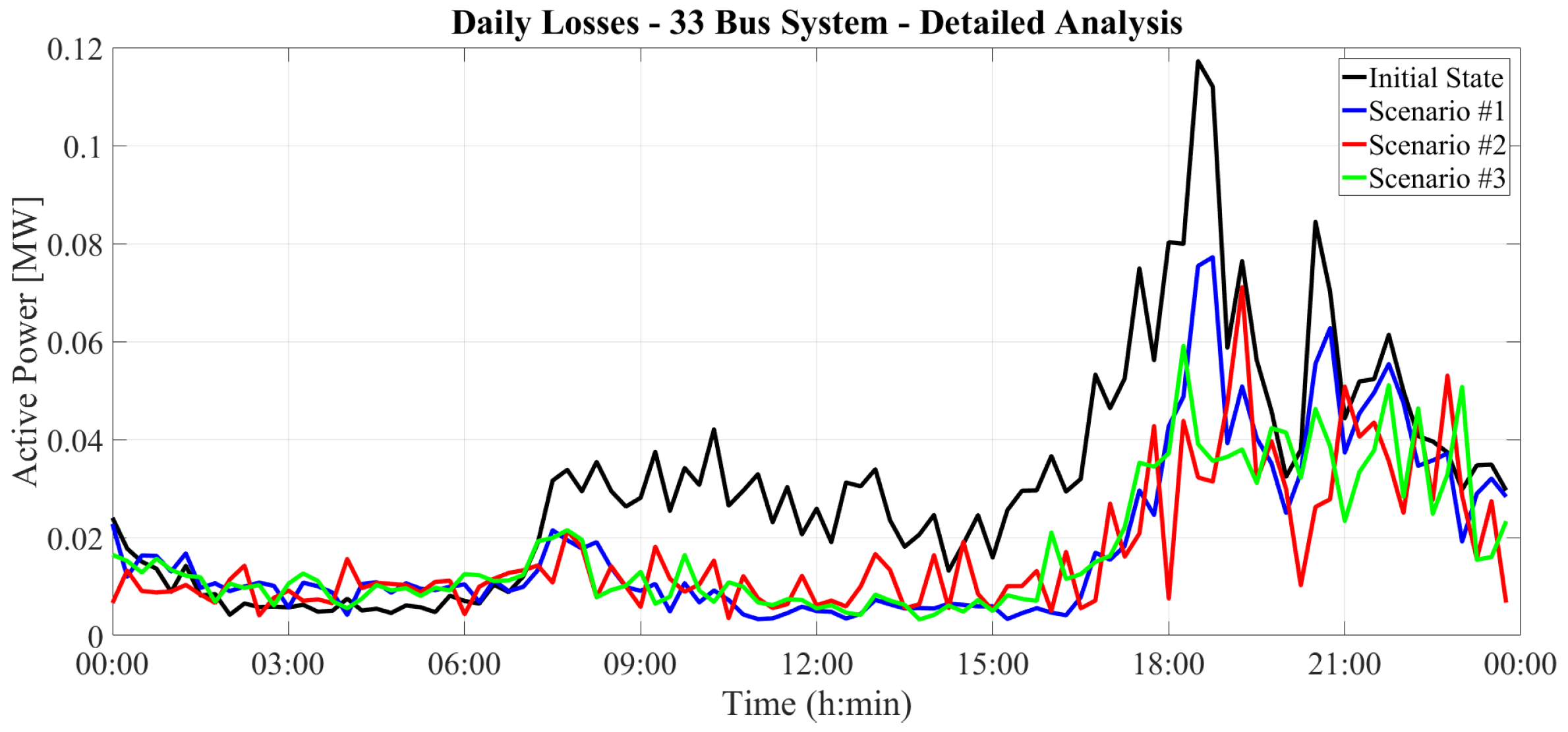
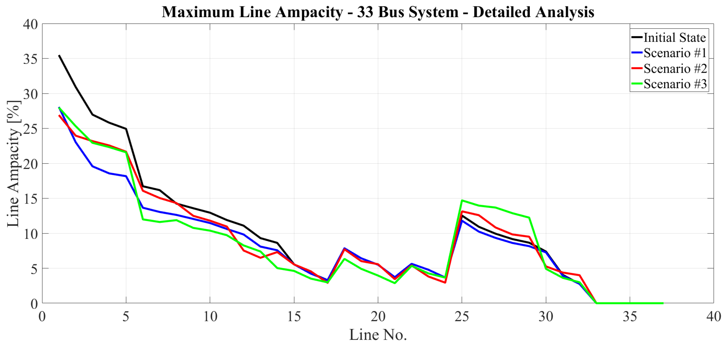
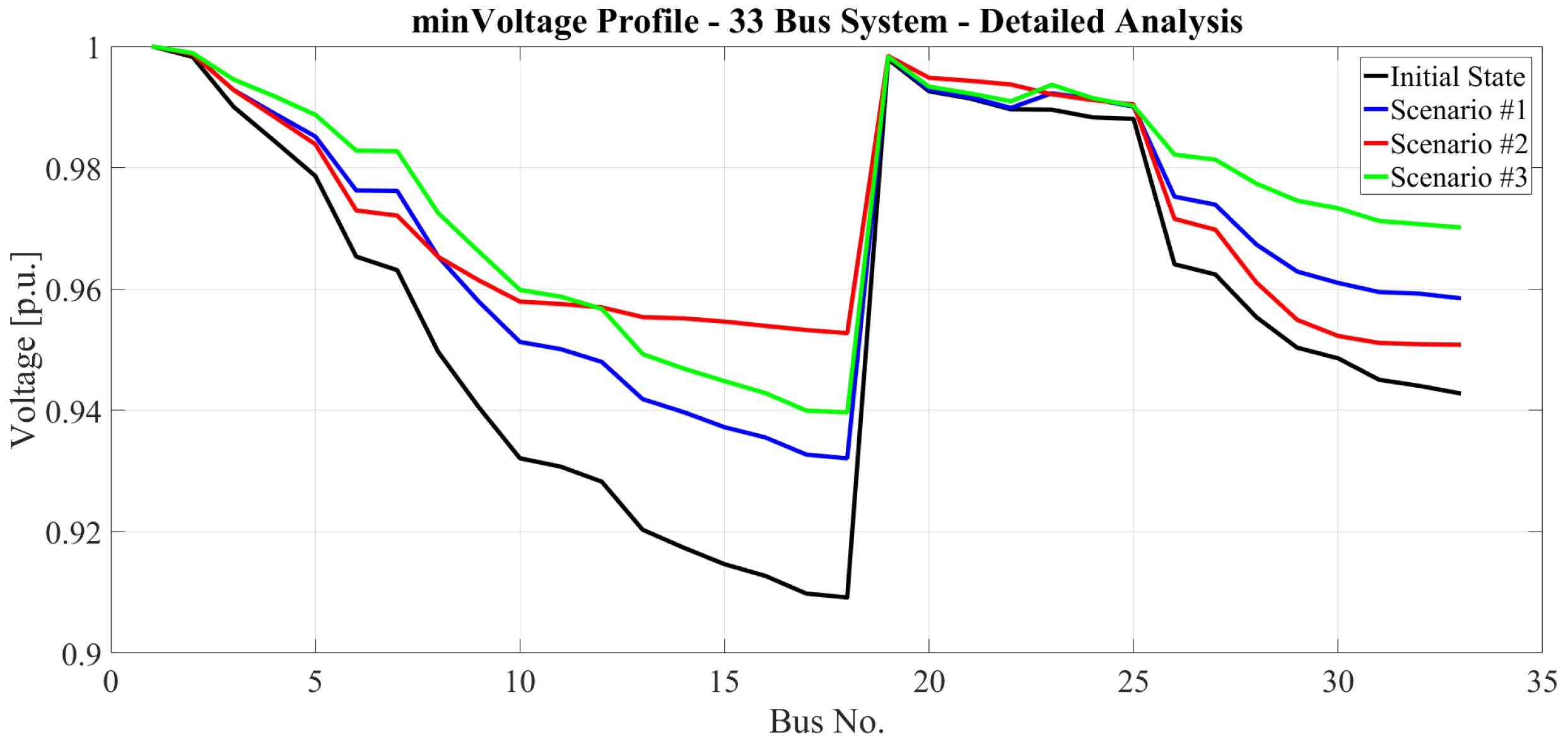
4. Detailed Analysis with Load and Generation Timeseries
- is the time interval considered and,
- is the total time period considered.
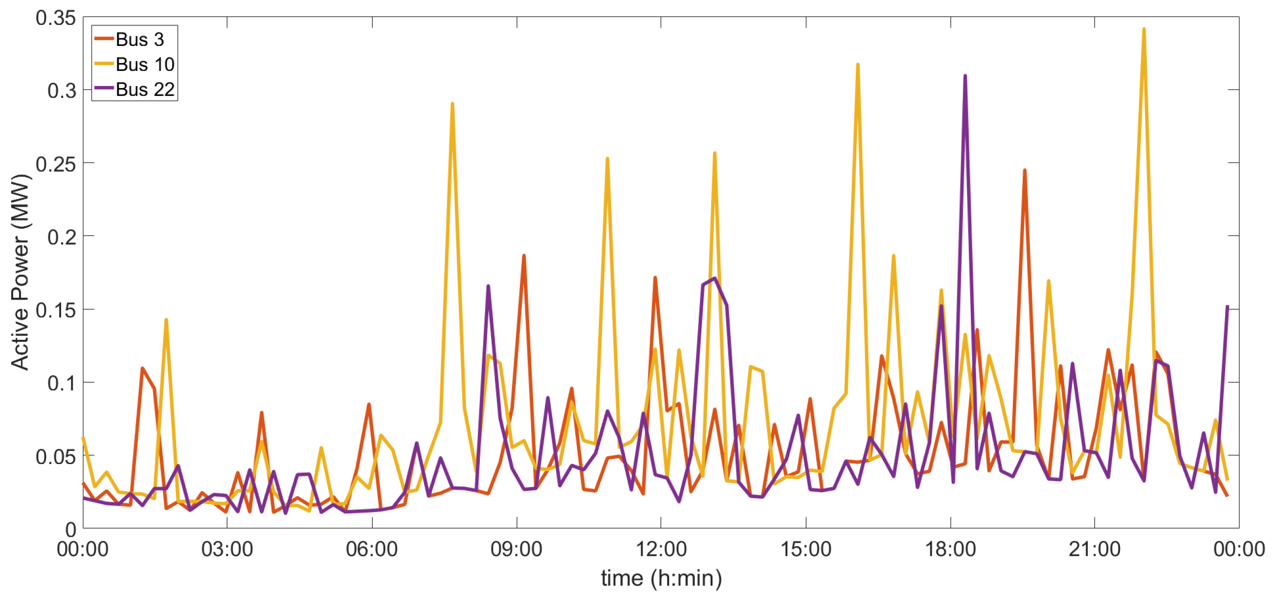
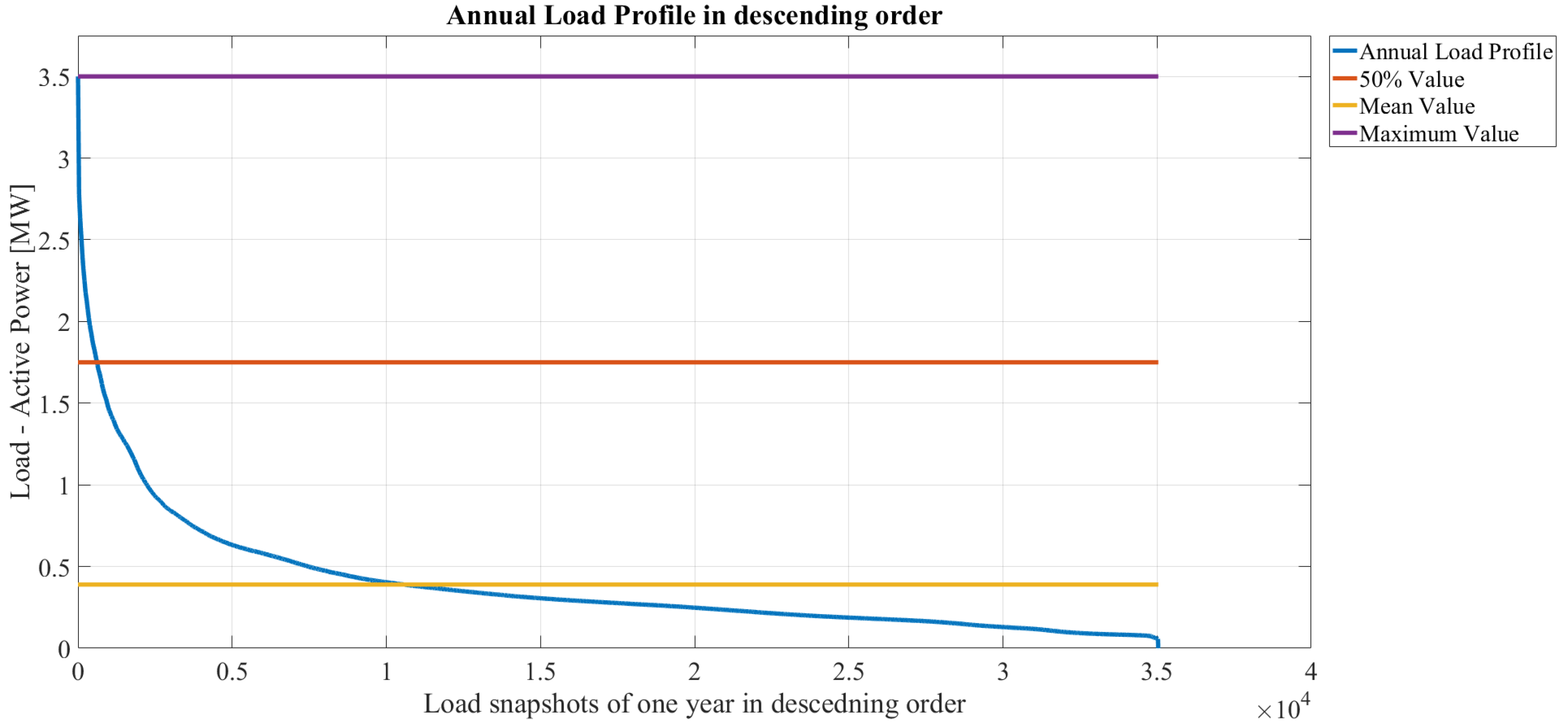
4.1. Load Variation
- the examined DN’s single snapshot is the annual DN’s load peak,
- the total DN load, as seen from the Slack Bus, follows the standard load profile’s pattern,
- the buses’ load profile follow their own random individual patterns, while not breaching any DN constraint, thus, no uniform load variations are considered, and,
- their total summation is equal to that seen from the Slack Bus, plus losses.
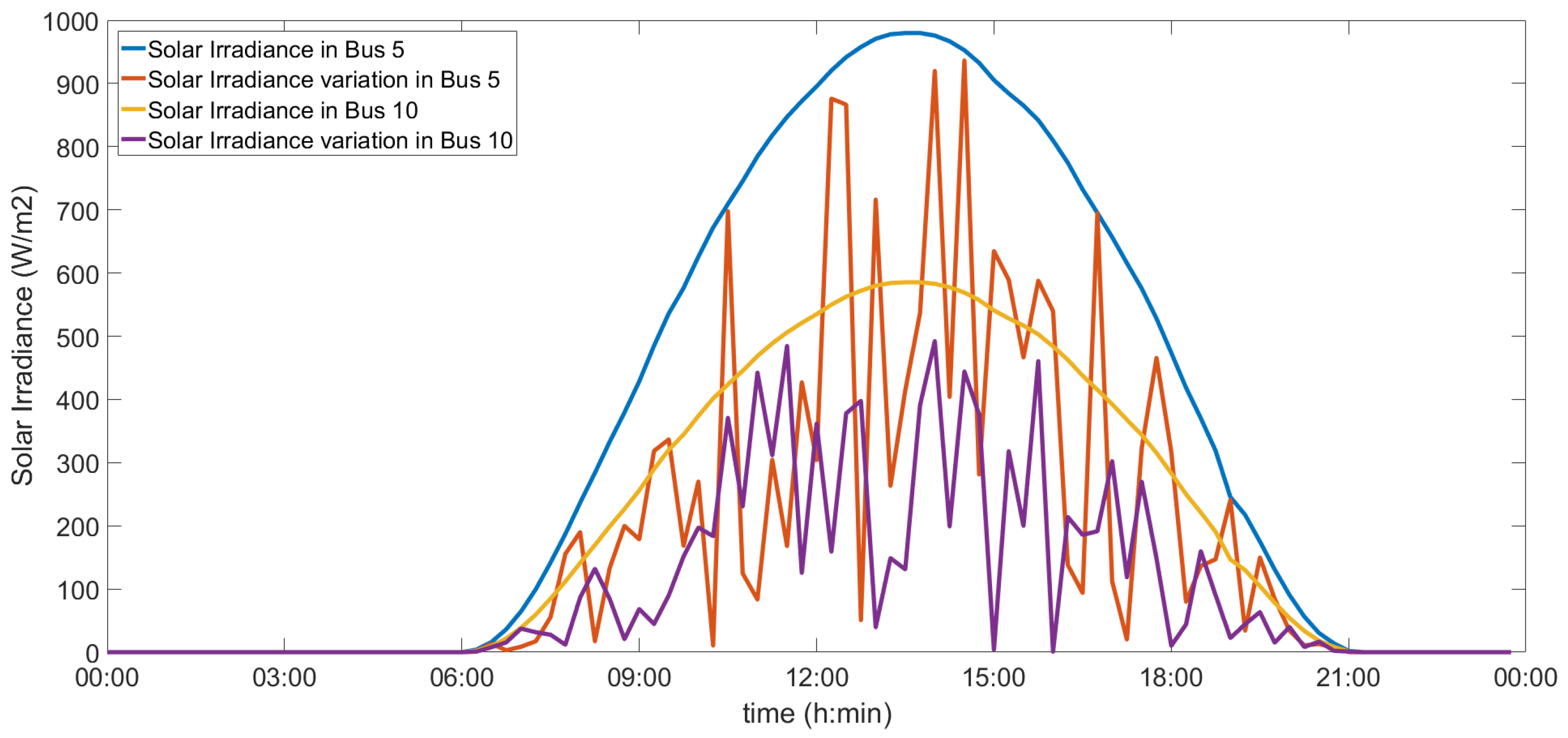
4.2. Generation Variation
4.2.1. PV
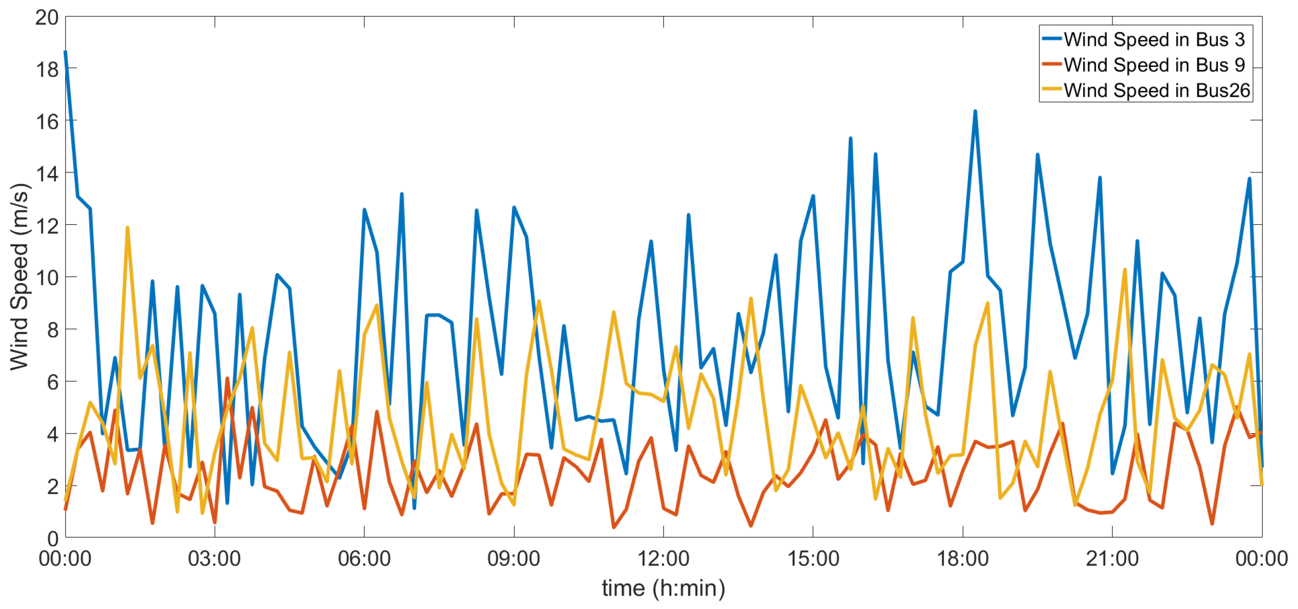
4.2.2. WP
- , is the power output of the WP unit according to the current wind speed,
- , is the rated power of the WP unit,
- , and are the cut-in, rated and cut-out speed of the WP unit, respectively.
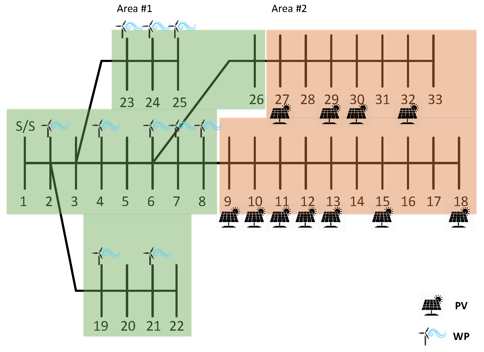
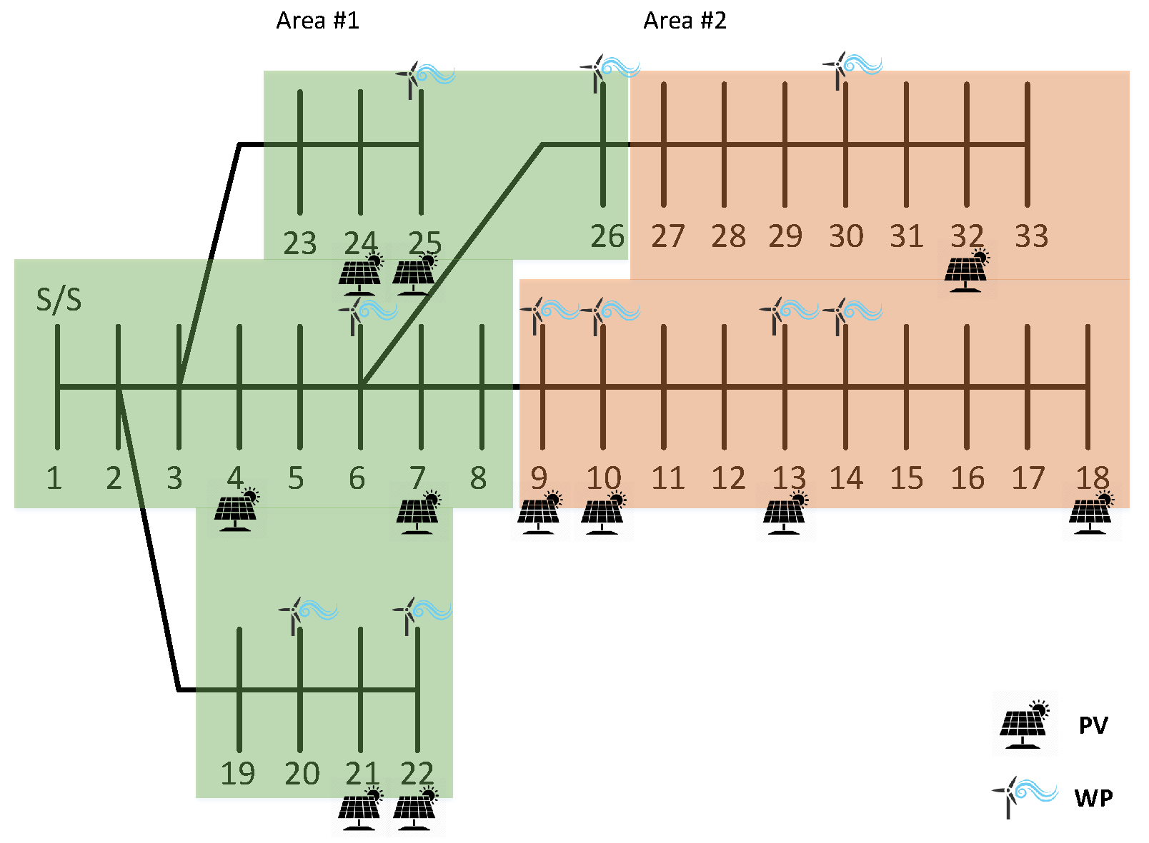
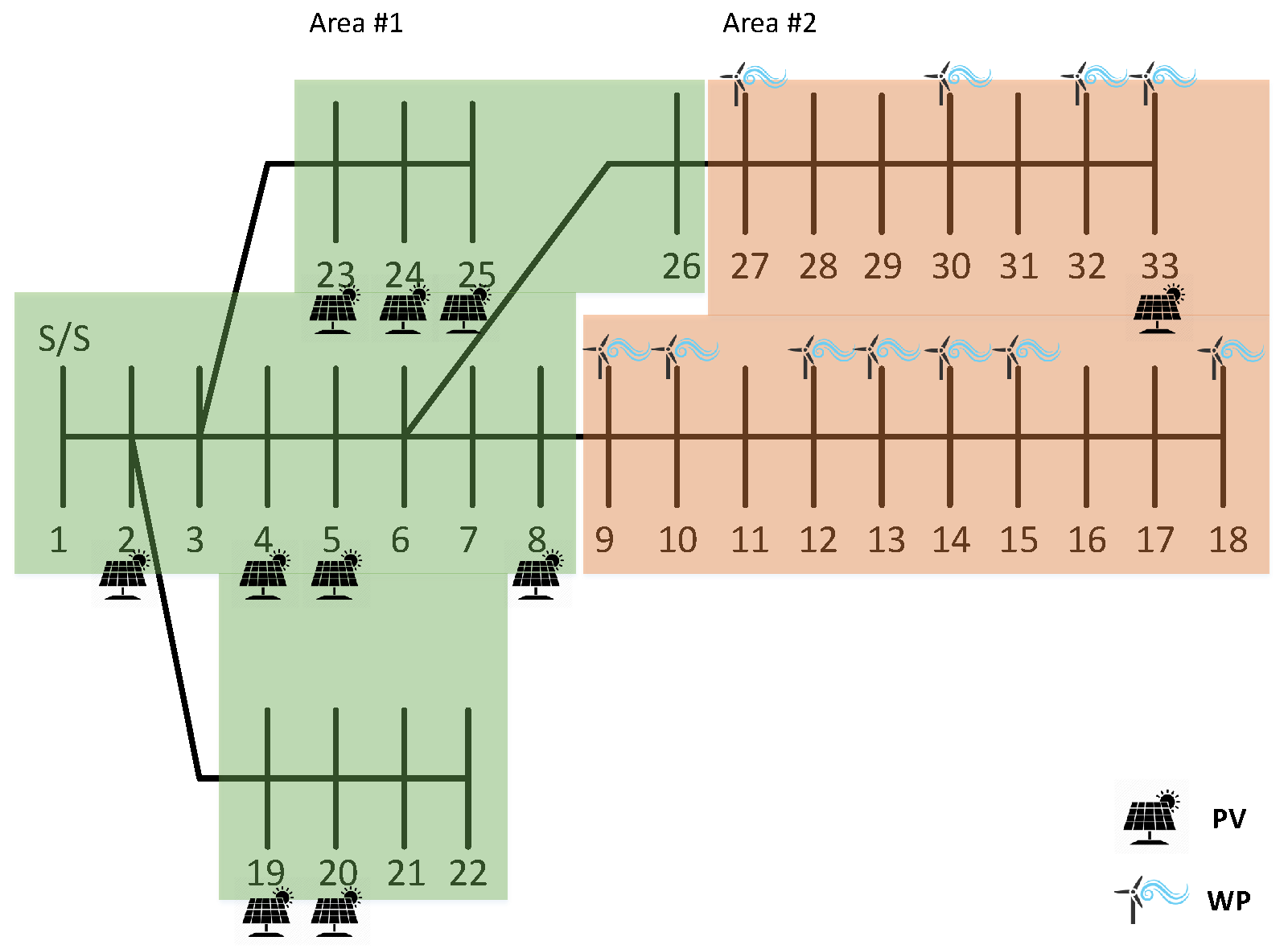
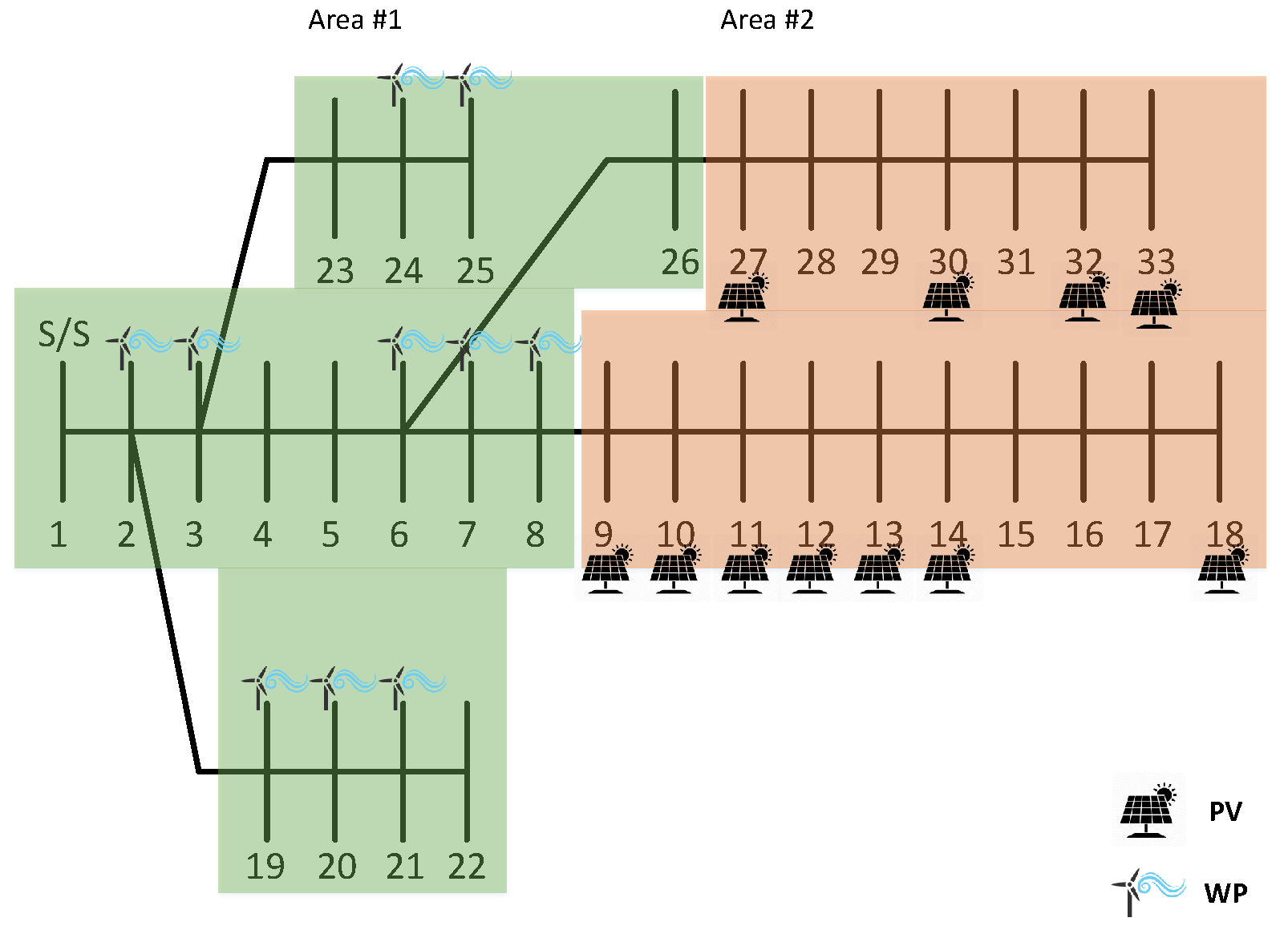
4.3. Implementation
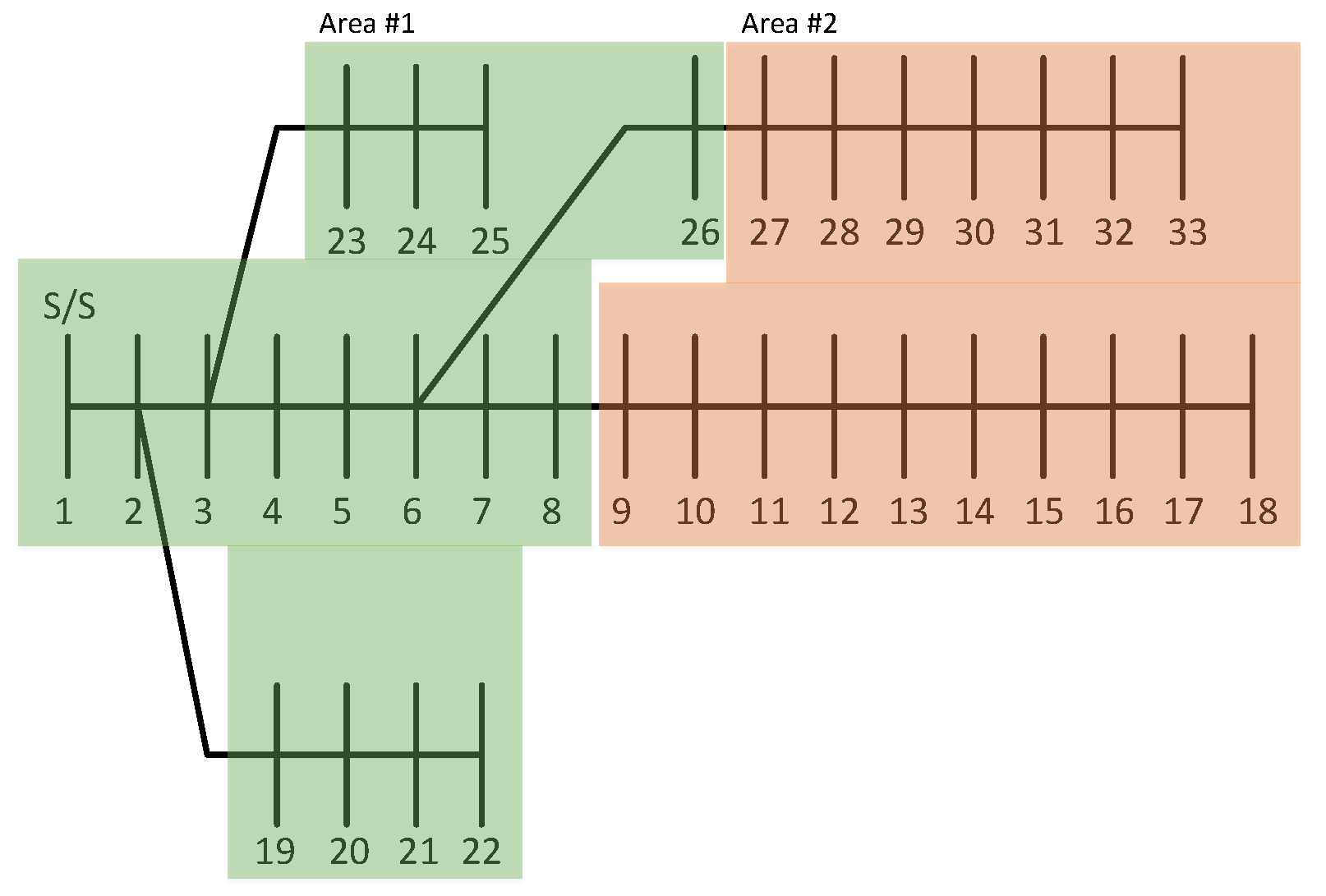
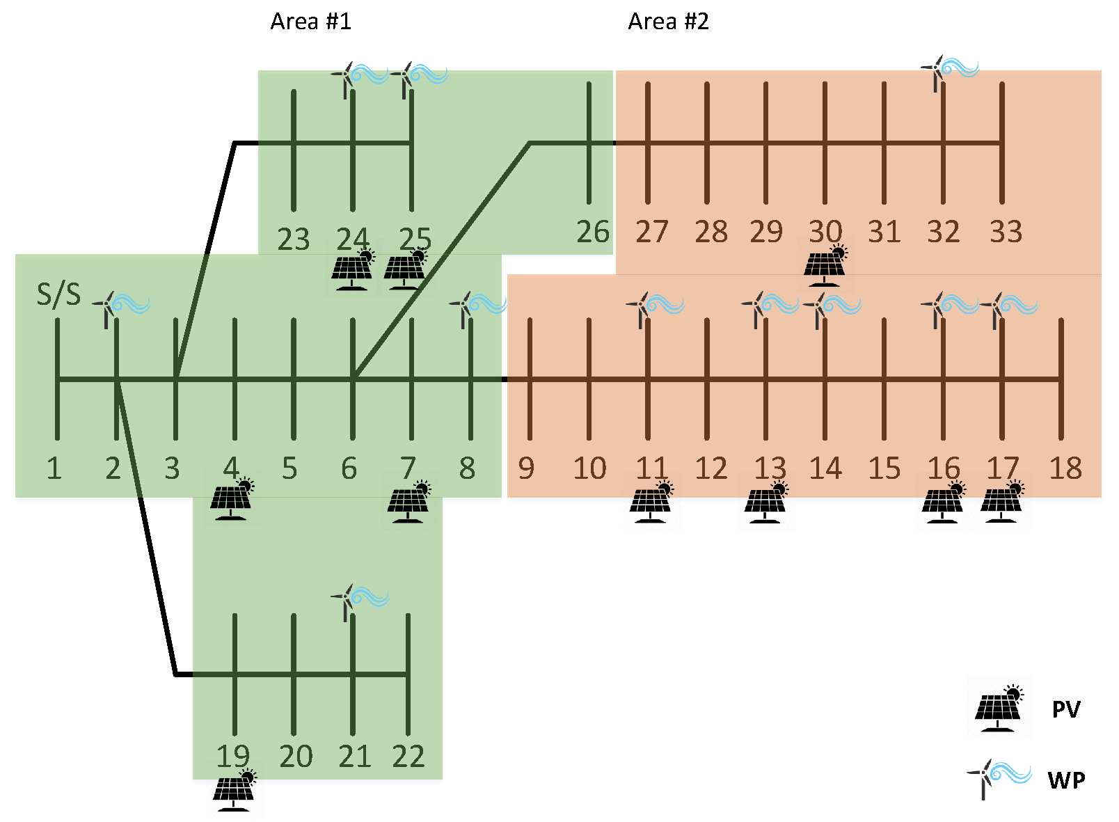
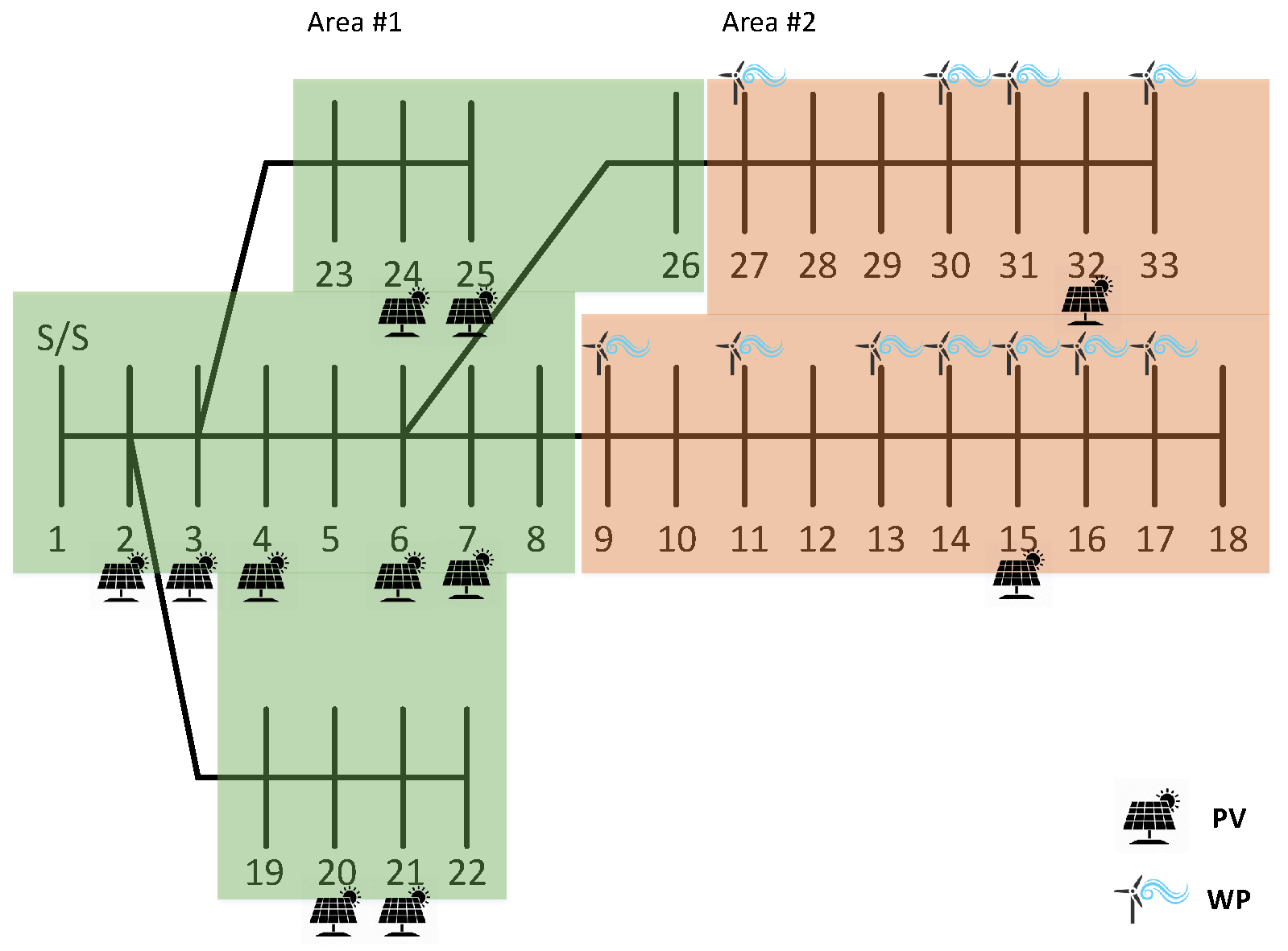
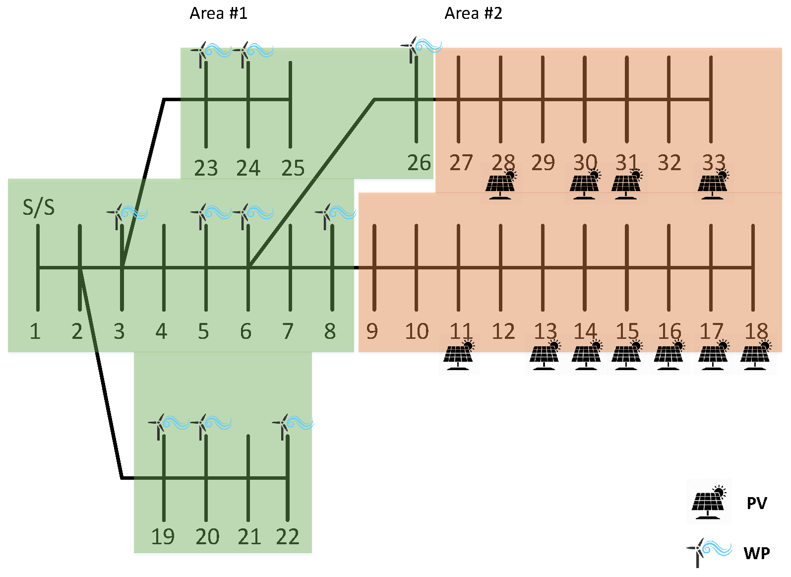
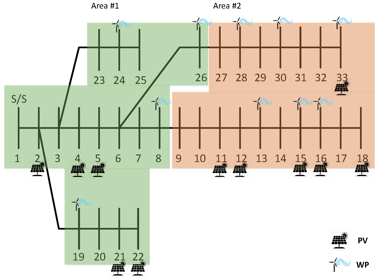
- Scenario #1: Area #1 has significantly better solar potential than wind potential, and Area #2 vice versa. Τhat is, in Area #1 PVs are promoted and in Area #2 WPs,
- Scenario #2: The opposite of Scenario #1, where Area #1 has significantly better wind potential than solar potential, and Area #2 vice versa. Τhat is, in Area #1 WPs are promoted and in Area #2 PVs, and,
- Scenario #3: Both Areas have good solar and wind potential. That is, in both areas PVs and WPs are promoted for installation.
5. Conclusions
Author Contributions
Funding
Conflicts of Interest
References
- Soroudi, A.; Ehsan, M.; Caire, R.; Hadjsaid, N. Hybrid immune-genetic algorithm method for benefit maximisation of distribution network operators and distributed generation owners in a deregulated environment. IET Gener. Transm. Distrib. 2011, 5, 961–972. [Google Scholar] [CrossRef]
- Kumar, M.; Nallagownden, P.; Elamvazuthi, I. Optimal Placement and Sizing of Renewable Distributed Generations and Capacitor Banks into Radial Distribution Systems. Energies 2017, 10, 811. [Google Scholar] [CrossRef]
- Esmaili, M. Placement of minimum distributed generation units observing power losses and voltage stability with network constraints. IET Gener. Transm. Distrib. 2013, 7, 813–821. [Google Scholar] [CrossRef]
- Abdmouleh, Z.; Gastli, A.; Ben-Brahim, L.; Haouari, M.; Al-Emadi, N.A. Review of optimization techniques applied for the integration of distributed generation from renewable energy sources. Renew. Energy 2017, 113, 266–280. [Google Scholar] [CrossRef]
- Tu, J.; Yin, Z.; Xu, Y. Study on the Evaluation Index System and Evaluation Method of Voltage Stability of Distribution Network with High DG Penetration. Energies 2018, 11, 79. [Google Scholar] [Green Version]
- Duong, M.Q.; Pham, T.D.; Nguyen, T.T.; Doan, A.T.; Tran, H.V. Determination of Optimal Location and Sizing of Solar Photovoltaic Distribution Generation Units in Radial Distribution Systems. Energies 2019, 12, 174. [Google Scholar] [CrossRef]
- Cetinay, H.; Kuipers, F.A.; Guven, A.N. Optimal siting and sizing of wind farms. Renew. Energy 2017, 101, 51–58. [Google Scholar] [CrossRef] [Green Version]
- Sanajaoba, S.; Fernandez, E. Maiden application of Cuckoo Search algorithm for optimal sizing of a remote hybrid renewable energy System. Renew. Energy 2016, 96, 1–10. [Google Scholar] [CrossRef]
- Vatu, R.; Ceaki, O.; Mancasi, M.; Porumb, R.; Seritan, G. Power quality issues produced by embedded storage technologies in smart grid environment. In Proceedings of the 2015 50th International Universities Power Engineering Conference (UPEC), Stoke on Trent, UK, 1–4 September 2015; pp. 1–5. [Google Scholar]
- Vatu, R.; Ceaki, O.; Golovanov, N.; Porumb, R.; Seritan, G. Analysis of storage technologies within smart grid framework. In Proceedings of the 2014 49th International Universities Power Engineering Conference (UPEC), Cluj-Napoca, Romania, 2–5 September 2014; pp. 1–5. [Google Scholar]
- Truong, A.V.; Ton, T.N.; Nguyen, T.T.; Duong, T.L. Two States for Optimal Position and Capacity of Distributed Generators Considering Network Reconfiguration for Power Loss Minimization Based on Runner Root Algorithm. Energies 2018, 12, 106. [Google Scholar] [CrossRef]
- Abu-Mouti, F.S.; El-Hawary, M.E. Optimal Distributed Generation Allocation and Sizing in Distribution Systems via Artificial Bee Colony Algorithm. IEEE Trans. Power Deliv. 2011, 26, 2090–2101. [Google Scholar] [CrossRef]
- El-Ela, A.A.A.; Allam, S.M.; Shatla, M.M. Maximal optimal benefits of distributed generation using genetic algorithms. Electr. Power Syst. Res. 2010, 80, 869–877. [Google Scholar] [CrossRef]
- Leeton, U.; Uthitsunthorn, D.; Kwannetr, U.; Sinsuphun, N.; Kulworawanichpong, T. Power loss minimization using optimal power flow based on particle swarm optimization. In Proceedings of the ECTI International Confernce on Electrical Engineering/Electronics, Computer, Telecommunications and Information Technology, Chiang Mai, Thailand, 19–21 May 2010; pp. 440–444. [Google Scholar]
- Kumar, T.; Thakur, T. Comparative analysis of particle swarm optimization variants on distributed generation allocation for network loss minimization. In Proceedings of the 1st International Confernce on Networks Soft Computing (ICNSC2014), Guntur, India, 19–20 August 2014; pp. 167–171. [Google Scholar]
- Hung, D.Q.; Mithulananthan, N.; Bansal, R.C. Analytical Expressions for DG Allocation in Primary Distribution Networks. IEEE Trans. Energy Convers. 2010, 25, 814–820. [Google Scholar] [CrossRef]
- Hung, D.Q.; Mithulananthan, N. Multiple Distributed Generator Placement in Primary Distribution Networks for Loss Reduction. IEEE Trans. Ind. Electron. 2013, 60, 1700–1708. [Google Scholar] [CrossRef]
- Abu-Mouti, F.S.; El-Hawary, M.E. Heuristic curve-fitted technique for distributed generation optimization in radial distribution feeder systems. IET Gener. Transm. Distrib. 2011, 5, 172–180. [Google Scholar] [CrossRef]
- Lee, S.H.; Park, J.W. Selection of Optimal Location and Size of Multiple Distributed Generations by Using Kalman Filter Algorithm. IEEE Trans. Power Syst. 2009, 24, 1393–1400. [Google Scholar]
- Moradi, M.; Abedini, M. A combination of genetic algorithm and particle swarm optimization for optimal DG location and sizing in distribution systems. Int. J. Electr. Power Energy Syst. 2012, 34, 66–74. [Google Scholar] [CrossRef]
- Moradi, M.H.; Reza Tousi, S.; Abedini, M. Multi-objective PFDE algorithm for solving the optimal siting and sizing problem of multiple DG sources. Int. J. Electr. Power Energy Syst. 2014, 56, 117–126. [Google Scholar] [CrossRef]
- Iyer, H.; Ray, S.; Ramakumar, R. Assessment of Distributed Generation Based on Voltage Profile Improvement and Line Loss Reduction. In Proceedings of the IEEE/PES Transmission and Distribution Conference and Exhibition, Dallas, TX, USA, 21–24 May 2006; pp. 1171–1176. [Google Scholar]
- Viral, R.; Khatod, D. An analytical approach for sizing and siting of DGs in balanced radial distribution networks for loss minimization. Int. J. Electr. Power Energy Syst. 2015, 67, 191–201. [Google Scholar] [CrossRef]
- Gkaidatzis, P.A.; Doukas, D.I.; Bouhouras, A.S.; Sgouras, K.I.; Labridis, D.P. Impact of penetration schemes to optimal DG placement for loss minimisation. Int. J. Sustain. Energy 2017, 36, 473–488. [Google Scholar] [CrossRef]
- Kayal, P.; Chanda, C. Placement of wind and solar based DGs in distribution system for power loss minimization and voltage stability improvement. Int. J. Electr. Power Energy Syst. 2013, 53, 795–809. [Google Scholar] [CrossRef]
- Pandi, V.R.; Zeineldin, H.H.; Xiao, W. Determining Optimal Location and Size of Distributed Generation Resources Considering Harmonic and Protection Coordination Limits. IEEE Trans. Power Syst. 2013, 28, 1245–1254. [Google Scholar] [CrossRef]
- Keane, A.; O’Malley, M. Optimal distributed generation plant mix with novel loss adjustment factors. In Proceedings of the IEEE Power Engineering Society General Meeting, Montreal, QC, Canada, 18–22 June 2006. [Google Scholar]
- Atwa, Y.M.; El-Saadany, E.F.; Salama, M.M.A.; Seethapathy, R. Optimal Renewable Resources Mix for Distribution System Energy Loss Minimization. IEEE Trans. Power Syst. 2010, 25, 360–370. [Google Scholar] [CrossRef]
- Yammani, C.; Maheswarapu, S.; Matam, S. Optimal placement of multi DGs in distribution system with considering the DG bus available limits. Energy Power 2012, 2, 18–23. [Google Scholar] [CrossRef]
- Parsopoulos, K.E.; Vrahatis, M.N. Particle Swarm Optimization and Intelligence: Advances and Applications; Information Science Reference: Hershey, PA, USA, 2010; pp. 25–41. [Google Scholar]
- Zimmerman, R.D.; Murillo-Sanchez, C.E.; Thomas, R.J. MATPOWER: Steady-State Operations, Planning, and Analysis Tools for Power Systems Research and Education. IEEE Trans. Power Syst. 2011, 26, 12–19. [Google Scholar] [CrossRef] [Green Version]
- Floudas, C.A.; Pardalos, P.M. A Collection of Test Problems for Constrained Global Optimization Algorithms; Springer Science & Business Media: Berlin, Germany, 1990; Volume 455. [Google Scholar]
- Hock, W.; Schittkowski, K. Test examples for nonlinear programming codes. J. Optim. Theory Appl. 1980, 30, 127–129. [Google Scholar] [CrossRef]
- Parsopoulos, K.E.; Vrahatis, M.N. Particle swarm optimization method for constrained optimization problems. In Intelligent Technologies—Theory and Application: New Trends in Intelligent Technologies; IOS Press: Hershey, NY, USA, 2002; Volume 76, pp. 214–220. [Google Scholar]
- Gkaidatzis, P.A.; Bouhouras, A.S.; Doukas, D.I.; Sgouras, K.I.; Labridis, D.P. Application and evaluation of UPSO to ODGP in radial Distribution Networks. In Proceedings of the 13th International Conference on the European Energy Market (EEM), Porto, Portugal, 6–9 June 2016; pp. 1–5. [Google Scholar]
- Gkaidatzis, P.A.; Doukas, D.I.; Labridis, D.P.; Bouhouras, A.S. Comparative analysis of heuristic techniques applied to ODGP. In Proceedings of the 2017 IEEE International Conference on Environment and Electrical Engineering and 2017 IEEE Industrial and Commercial Power Systems Europe (EEEIC/I CPS Europe), Milan, Italy, 6–9 June 2017; pp. 1–6. [Google Scholar]
- Kashem, M.A.; Ganapathy, V.; Jasmon, G.B.; Buhari, M.I. A novel method for loss minimization in distribution networks. In Proceedings of the International Conference on Electric Utility Deregulation and Restructuring and Power Technologies, Proceedings (Cat. No.00EX382), London, UK, 4–7 April 2000; pp. 251–256. [Google Scholar]
- Warkad, S.B.; Khedkar, M.K.; Dhole, G.M. Economics of AC-DC OPF Based Nodal Prices for Restructured Electric Power System. Int. J. Electr. Power Eng. 2009, 3, 276–288. [Google Scholar]
- Salameh, Z.M.; Borowy, B.S.; Amin, A.R.A. Photovoltaic module-site matching based on the capacity factors. IEEE Trans. Energy Convers. 1995, 10, 326–332. [Google Scholar] [CrossRef]
- Ackermann, T. Wind Power in Power Systems; John Wiley & Sons: West Sussex, UK, 2005. [Google Scholar]
- Lako, P. Technical and Economic Features of Renewable Electricity Technologies; Technical Report; Energy Research Centre of The Netherlands: Petten, The Netherlands, 2010. [Google Scholar]
- Standard Load Profiles | RMDS. Available online: https://rmdservice.com/standard-load-profiles/ (accessed on 30 March 2019).
- Solar Radiation Data—Solar Energy Services for Professionals. Available online: http://www.soda-is.com/eng/services/services_radiation_free_eng.php (accessed on 30 March 2019).
- Tu, J.; Xu, Y.; Yin, Z. Data-Driven Kernel Extreme Learning Machine Method for the Location and Capacity Planning of Distributed Generation. Energies 2019, 12, 109. [Google Scholar] [CrossRef]
- Hennessey, J.P., Jr. A comparison of the Weibull and Rayleigh distributions for estimating wind power potential. Wind Eng. 1978, 2, 156–164. [Google Scholar]
- Turitsyn, K.; Sulc, P.; Backhaus, S.; Chertkov, M. Options for Control of Reactive Power by Distributed Photovoltaic Generators. Proc. IEEE 2011, 99, 1063–1073. [Google Scholar] [CrossRef] [Green Version]
- Zhao, H.; Wu, Q.; Wang, J.; Liu, Z.; Shahidehpour, M.; Xue, Y. Combined Active and Reactive Power Control of Wind Farms Based on Model Predictive Control. IEEE Trans. Energy Convers. 2017, 32, 1177–1187. [Google Scholar] [CrossRef]
- Collins, L.; Ward, J. Real and reactive power control of distributed PV inverters for overvoltage prevention and increased renewable generation hosting capacity. Renew. Energy 2015, 81, 464–471. [Google Scholar] [CrossRef]


| Area | RES Technology | ||
|---|---|---|---|
| WP | PV | HD | |
| Area #1 | 0.28 | 0.10 | 0.00 |
| Area #2 | 0.00 | 0.15 | 0.00 |
| Area #3 | 0.14 | 0.10 | 0.45 |
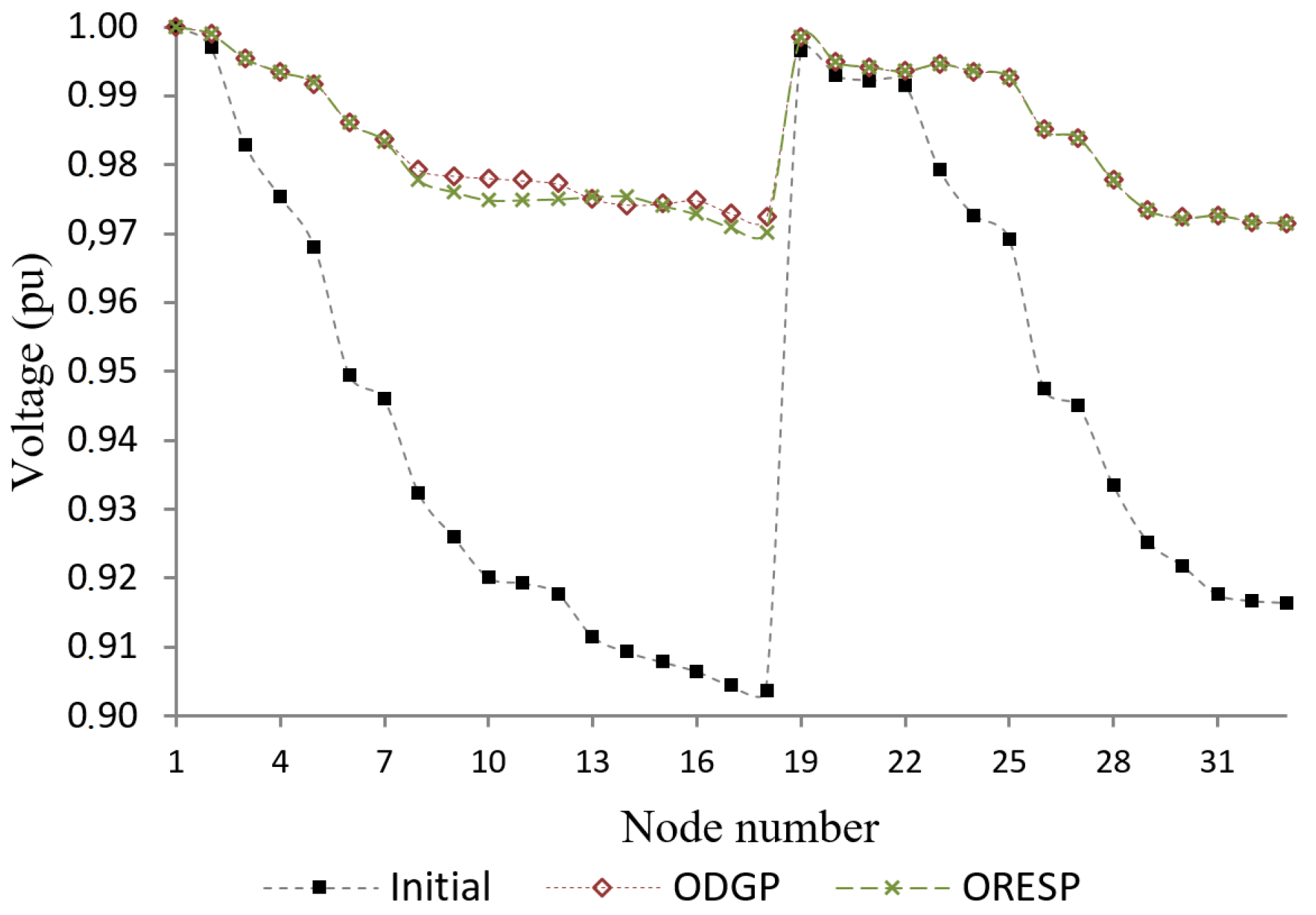
| ODGP—33 Bus System | ||||||||
|---|---|---|---|---|---|---|---|---|
| Initial losses | Loss reduction | Aggregated DG capacity | ||||||
| 211 kW | 69.06% | 3.22 MW | ||||||
| DG hosting node number and power (kW) | ||||||||
| Bus No. | 6 | 10 | 16 | 24 | 25 | 31 | ||
| DG Size (kW) | 792.3 | 392.8 | 379.2 | 543.8 | 420.8 | 687.9 | ||
| ORESP—33 Bus System | ||||||||
|---|---|---|---|---|---|---|---|---|
| Initial losses | Loss reduction | Aggregated DG capacity | ||||||
| 211 kW | 68.43% | 3.22 MW | ||||||
| RES hosting node number and power (kW) | ||||||||
| Bus No. | 6 | 14 | 24 | 25 | 31 | |||
| RES type | WP | WP | PV | PV | HD | |||
| RES Size (kW) | 926.3 | 646.8 | 545.0 | 420.2 | 686.4 | |||
| ODGP—118 Bus System | ||||||||||||
|---|---|---|---|---|---|---|---|---|---|---|---|---|
| Initial losses | Loss reduction | Aggregated DG capacity | ||||||||||
| 132.86 MW | 31.99% | 755.39 MW | ||||||||||
| DG hosting node number and power (MW) | ||||||||||||
| Bus No. | 1 | 2 | 20 | 28 | 31 | 40 | 42 | 43 | 44 | 45 | 52 | |
| DG Size (kW) | 10.90 | 19.26 | 16.85 | 18.77 | 92.48 | 70.99 | 21.11 | 0.54 | 43.11 | 15.53 | 15.47 | |
| Bus No. | 53 | 54 | 56 | 70 | 74 | 76 | 107 | 112 | 117 | 118 | ||
| DG Size (kW) | 11.91 | 47.69 | 97.56 | 34.92 | 76.22 | 35.65 | 28.78 | 47.07 | 9.50 | 41.08 | ||
| ORESP—118 Bus System | |||||||||||
|---|---|---|---|---|---|---|---|---|---|---|---|
| Initial losses | Loss reduction | Aggregated DG capacity | |||||||||
| 132.86 kW | 24.71% | 659.12 MW | |||||||||
| RES hosting node number, type, and power (MW) | |||||||||||
| Bus No. | 1 | 2 | 19 | 21 | 95 | 97 | 98 | 102 | 16 | 33 | 34 |
| RES type | WP | WP | WP | WP | WP | WP | WP | WP | PV | PV | PV |
| RES Size (kW) | 11.11 | 12.80 | 9.54 | 1.56 | 6.45 | 5.26 | 5.35 | 4.86 | 0.04 | 2.93 | 0.60 |
| Bus No. | 40 | 41 | 42 | 54 | 59 | 63 | 84 | 98 | 112 | 118 | 24 |
| RES type | PV | PV | PV | PV | PV | PV | PV | PV | PV | PV | HD |
| RES Size (kW) | 2.20 | 105.02 | 14.98 | 216.87 | 4.15 | 2.45 | 3.38 | 0.94 | 21.51 | 0.07 | 3.97 |
| Bus No. | 34 | 38 | 70 | 83 | 88 | 94 | 95 | 103 | 104 | 112 | |
| RES type | HD | HD | HD | HD | HD | HD | HD | HD | HD | HD | |
| RES Size (kW) | 20.49 | 11.81 | 138.73 | 2.72 | 0.21 | 2.36 | 3.34 | 0.20 | 29.48 | 13.75 | |
| Initial | ODGP | ORESP | |
|---|---|---|---|
| Average voltage (p.u.) | 0.9857 | 0.9867 | 0.9862 |
| Scenario | RES Technology | |
|---|---|---|
| PV | WP | |
| #1 | Area #1 | Area #2 |
| #2 | Area #2 | Area #1 |
| #3 | Both Areas | Both Areas |
| PV | WP | ||||||||
|---|---|---|---|---|---|---|---|---|---|
| Bus No. | P (kW) | Q (kVAr) | Area No. | CF | Bus No. | P (kW) | Q (kVAr) | Area No. | CF |
| 3 | 427.16 | 24.32 | 1 | 18.07 | 10 | 0.00 | 90.11 | 2 | 35.43 |
| 4 | 0.00 | 8.00 | 1 | 18.19 | 11 | 343.36 | 4.28 | 2 | 38.04 |
| 6 | 645.00 | 23.35 | 1 | 18.12 | 17 | 240.55 | 0.93 | 2 | 39.27 |
| 7 | 0.00 | 0.13 | 1 | 18.28 | 30 | 377.93 | 267.84 | 2 | 38.94 |
| 14 | 589.81 | 33.25 | 2 | 10.98 | |||||
| 16 | 5.03 | 47.05 | 2 | 10.89 | |||||
| 21 | 218.46 | 0.00 | 1 | 18.23 | |||||
| Total No. | Total P (kW) | Total Q (kVAr) | Total No. | Total P (kW) | Total Q (kVAr) | ||||
| 7 | 1885.46 | 136.10 | 4 | 961.85 | 363.15 | ||||
| Total RES No. | Total RES P (kW) | Total RES Q (kVAr) | |||||||
| 11 | 2847.31 | 499.25 | |||||||
| Initial Energy Losses (MWh) | Optimal Energy Losses (MWh) | Energy Loss Reduction (%) | |||||||
| 5397.17 | 2601.79 | −51.85 | |||||||
| PV | WP | ||||||||
|---|---|---|---|---|---|---|---|---|---|
| Bus No. | P (kW) | Q (kVAr) | Area No. | CF | Bus No. | P (kW) | Q (kVAr) | Area No. | CF |
| 3 | 429.47 | 215.49 | 1 | 10.86 | 3 | 270.87 | 223.67 | 2 | 37.23 |
| 6 | 0.00 | 0.13 | 1 | 10.82 | 5 | 177.78 | 0.00 | 2 | 38.83 |
| 11 | 221.30 | 114.86 | 2 | 18.11 | 6 | 375.30 | 124.82 | 2 | 34.37 |
| 15 | 409.77 | 0.00 | 2 | 18.07 | 8 | 547.76 | 20.16 | 2 | 37.49 |
| 17 | 0.00 | 76.04 | 2 | 18.00 | 20 | 195.47 | 0.00 | 2 | 38.83 |
| 30 | 374.16 | 247.72 | 2 | 18.19 | |||||
| 33 | 0.00 | 18.79 | 2 | 18.09 | |||||
| Total No. | Total P (kW) | Total Q (kVAr) | Total No. | Total P (kW) | Total Q (kVAr) | ||||
| 7 | 1434.70 | 673.02 | 5 | 1567.18 | 368.65 | ||||
| Total RES No. | Total RES P (kW) | Total RES Q (kVAr) | |||||||
| 12 | 3001.88 | 1041.68 | |||||||
| Initial Energy Losses (MWh) | Optimal Energy Losses (MWh) | Energy Loss Reduction (%) | |||||||
| 5397.17 | 2795.11 | −48.21 | |||||||
| PV | WP | ||||||||
|---|---|---|---|---|---|---|---|---|---|
| Bus No. | P (kW) | Q (kVAr) | Area No. | CF | Bus No. | P (kW) | Q (kVAr) | Area No. | CF |
| 3 | 302.00 | 240.30 | 1 | 18.22 | 4 | 138.10 | 201.44 | 1 | 37.45 |
| 7 | 0.00 | 185.93 | 1 | 18.23 | 5 | 0.00 | 0.34 | 1 | 34.83 |
| 8 | 286.26 | 0.69 | 1 | 18.22 | 6 | 295.82 | 0.00 | 1 | 38.30 |
| 15 | 329.57 | 83.68 | 2 | 18.02 | 9 | 2.59 | 35.75 | 2 | 34.72 |
| 30 | 292.83 | 239.42 | 2 | 18.05 | 11 | 271.94 | 64.90 | 2 | 38.66 |
| 13 | 89.00 | 0.00 | 2 | 38.86 | |||||
| 18 | 154.66 | 0.00 | 2 | 38.89 | |||||
| 33 | 207.03 | 0.00 | 2 | 38.60 | |||||
| Total No. | Total P (kW) | Total Q (kVAr) | Total No. | Total P (kW) | Total Q (kVAr) | ||||
| 5 | 1210.66 | 750.03 | 8 | 1159.15 | 302.43 | ||||
| Total RES No. | Total RES P (kW) | Total RES Q (kVAr) | |||||||
| 13 | 2369.81 | 1052.45 | |||||||
| Initial Energy Losses (MWh) | Optimal Energy Losses (MWh) | Energy Loss Reduction (%) | |||||||
| 5397.17 | 2587.14 | −51.98 | |||||||
| Scenario | Area#1 | Area#2 | ||
|---|---|---|---|---|
| PV | WP | PV | WP | |
| #1 | 17.56% | 0.00% | 10.69% | 38.17% |
| #2 | 10.69% | 38.17% | 17.56% | 0.00% |
| #3 | 17.56% | 38.17% | 17.56% | 38.17% |
| PV | WP | |||||||
|---|---|---|---|---|---|---|---|---|
| Bus No. | P (kW) | Q (kVAr) | Area No. | Bus No. | P (kW) | Q (kVAr) | Area No. | |
| 2 | 0.00 | −5.61 | 1 | 9 | 228.35 | 100.90 | 2 | |
| 3 | 207.00 | 133.58 | 1 | 10 | 0.00 | −11.25 | 2 | |
| 4 | 0.00 | 21.72 | 1 | 11 | 0.00 | 4.2 | 2 | |
| 5 | 180.65 | 33.13 | 1 | 12 | 236.15 | 123.26 | 2 | |
| 6 | 369.35 | 169.18 | 1 | 15 | 0.00 | 37.60 | 2 | |
| 15 | 481.38 | −601.25 | 2 | 16 | 351.61 | 129.60 | 2 | |
| 19 | 106.10 | 49.65 | 1 | 27 | 19.49 | 42.62 | 2 | |
| 20 | 121.32 | 36.90 | 1 | 28 | 98.58 | 1.40 | 2 | |
| 21 | 157.54 | 82.85 | 1 | 29 | 88.85 | 111.98 | 2 | |
| 24 | 455.06 | 183.51 | 1 | 30 | 254.59 | 574.15 | 2 | |
| 25 | 410.37 | 224.80 | 1 | 31 | 382.83 | 207.11 | 2 | |
| Total No. | Total P (kW) | Total Q (kVAr) | Total No. | Total P (kW) | Total Q (kVAr) | |||
| 11 | 2488.75 | 328.46 | 11 | 1660.44 | 1321.58 | |||
| Total RES No. | Total RES P (kW) | Total RES Q (kVAr) | ||||||
| 22 | 4149.20 | 1650.04 | ||||||
| Initial Energy Losses (MWh) | Optimal Energy Losses (MWh) | Energy Loss Reduction (%) | ||||||
| 5397.17 | 6525.83 | +20.78 | ||||||
| PV | WP | |||||||
|---|---|---|---|---|---|---|---|---|
| Bus No. | P (kW) | Q (kVAr) | Area No. | Bus No. | P (kW) | Q (kVAr) | Area No. | |
| 9 | 0.00 | 41.49 | 2 | 2 | 0.00 | 60.25 | 1 | |
| 10 | 205.80 | −81.56 | 2 | 4 | 0.00 | 82.32 | 1 | |
| 11 | 0.00 | 288.34 | 2 | 6 | 260.98 | 68.46 | 1 | |
| 12 | 0.00 | −164.95 | 2 | 7 | 153.22 | 74.85 | 1 | |
| 13 | 0.00 | 103.33 | 2 | 8 | 251.20 | 94.39 | 1 | |
| 15 | 271.96 | 78.74 | 2 | 19 | 207.48 | 45.30 | 1 | |
| 18 | 152.06 | 54.95 | 2 | 21 | 239.88 | 108.58 | 1 | |
| 27 | 123.88 | 29.11 | 2 | 23 | 185.81 | 145.84 | 1 | |
| 29 | 0.00 | 118.38 | 2 | 24 | 429.26 | 163.78 | 1 | |
| 30 | 351.27 | 590.80 | 2 | 25 | 410.27 | 193.32 | 1 | |
| 32 | 384.29 | 192.87 | 2 | |||||
| Total No. | Total P (kW) | Total Q (kVAr) | Total No. | Total P (kW) | Total Q (kVAr) | |||
| 11 | 1489.24 | 1251.49 | 10 | 2138.10 | 1037.11 | |||
| Total RES No. | Total RES P (kW) | Total RES Q (kVAr) | ||||||
| 21 | 3627.34 | 2288.60 | ||||||
| Initial Energy Losses (MWh) | Optimal Energy Losses (MWh) | Energy Loss Reduction (%) | ||||||
| 5397.17 | 7906.66 | +46.50 | ||||||
| PV | WP | |||||||
|---|---|---|---|---|---|---|---|---|
| Bus No. | P (kW) | Q (kVAr) | Area No. | Bus No. | P (kW) | Q (kVAr) | Area No. | |
| 4 | 229.22 | 138.26 | 1 | 6 | 135.67 | 133.00 | 1 | |
| 7 | 242.77 | 74.90 | 1 | 9 | 191.17 | 89.33 | 2 | |
| 9 | 429.13 | 73.30 | 2 | 10 | 136.92 | 69.69 | 2 | |
| 10 | 1113.36 | −326.92 | 2 | 13 | 82.47 | 46.30 | 2 | |
| 13 | 563.41 | 133.97 | 2 | 14 | 218.43 | 105.12 | 2 | |
| 18 | 171.79 | 66.04 | 2 | 19 | 309.13 | 67.36 | 1 | |
| 20 | 75.01 | 40.09 | 1 | 21 | 172.65 | 80.60 | 1 | |
| 21 | 45.80 | −380.91 | 1 | 25 | 420.26 | 197.66 | 1 | |
| 24 | 468.65 | 231.52 | 1 | 26 | 141.83 | 31.45 | 1 | |
| 25 | 863.77 | −486.96 | 1 | 30 | 378.56 | 687.04 | 2 | |
| 32 | 377.78 | 193.35 | 2 | |||||
| Total No. | Total P (kW) | Total Q (kVAr) | Total No. | Total P (kW) | Total Q (kVAr) | |||
| 11 | 4580.70 | −243.35 | 10 | 2187.10 | 1507.55 | |||
| Total RES No. | Total RES P (kW) | Total RES Q (kVAr) | ||||||
| 21 | 6767.80 | 1264.20 | ||||||
| Initial Energy Losses (MWh) | Optimal Energy Losses (MWh) | Energy Loss Reduction (%) | ||||||
| 5397.17 | 8504.35 | +57.85 | ||||||
| PV | WP | |||||||
|---|---|---|---|---|---|---|---|---|
| Bus No. | P (kW) | Q (kVAr) | Area No. | Bus No. | P (kW) | Q (kVAr) | Area No. | |
| 2 | 100.40 | −1.23 | 1 | 9 | 24.64 | 18.97 | 2 | |
| 4 | 129.68 | 51.93 | 1 | 10 | 83.97 | −17.58 | 2 | |
| 5 | 0.00 | 33.76 | 1 | 12 | 0.00 | 54.25 | 2 | |
| 8 | 132.23 | 64.48 | 1 | 13 | 9.28 | 16.16 | 2 | |
| 19 | 0.00 | 47.10 | 1 | 14 | 108.57 | 27.08 | 2 | |
| 20 | 138.60 | 56.82 | 1 | 15 | 34.60 | 24.17 | 2 | |
| 23 | 66.59 | 21.69 | 1 | 18 | 76.08 | 31.30 | 2 | |
| 24 | 159.93 | 120.82 | 1 | 27 | 164.60 | 61.88 | 2 | |
| 25 | 253.92 | 88.43 | 1 | 30 | 180.72 | 346.38 | 2 | |
| 33 | 320.10 | 201.15 | 2 | 32 | 139.34 | 66.75 | 2 | |
| 33 | 50.35 | 24.73 | 2 | |||||
| Total No. | Total P (kW) | Total Q (kVAr) | Total No. | Total P (kW) | Total Q (kVAr) | |||
| 11 | 1301.56 | 684.95 | 11 | 872.17 | 654.09 | |||
| Total RES No. | Total RES P (kW) | Total RES Q (kVAr) | ||||||
| 21 | 2173.73 | 1339.04 | ||||||
| Initial Energy Losses (MWh) | Optimal Energy Losses (MWh) | Energy Loss Reduction (%) | ||||||
| 5397.17 | 4473.61 | −17.20 | ||||||
| PV | WP | |||||||
|---|---|---|---|---|---|---|---|---|
| Bus No. | P (kW) | Q (kVAr) | Area No. | Bus No. | P (kW) | Q (kVAr) | Area No. | |
| 9 | 0.00 | 1.24 | 2 | 2 | 169.03 | 40.39 | 1 | |
| 10 | 0.00 | 8.12 | 2 | 3 | 0.00 | 66.70 | 1 | |
| 11 | 0.00 | 19.38 | 2 | 6 | 18.36 | 18.95 | 1 | |
| 12 | 87.32 | 20.30 | 2 | 7 | 128.08 | 57.86 | 1 | |
| 13 | 2.27 | 0.17 | 2 | 8 | 132.22 | 59.58 | 1 | |
| 14 | 133.97 | 70.18 | 2 | 19 | 0.00 | 10.89 | 1 | |
| 18 | 85.27 | 29.32 | 2 | 20 | 130.50 | 25.06 | 1 | |
| 27 | 121.13 | 39.52 | 2 | 21 | 11.84 | 37.68 | 1 | |
| 30 | 171.42 | 336.53 | 2 | 24 | 249.75 | 117.88 | 1 | |
| 32 | 192.83 | 83.85 | 2 | 25 | 214.67 | 91.70 | 1 | |
| 33 | 0.00 | 13.35 | 2 | |||||
| Total No. | Total P (kW) | Total Q (kVAr) | Total No. | Total P (kW) | Total Q (kVAr) | |||
| 11 | 794.21 | 621.95 | 10 | 1054.44 | 526.70 | |||
| Total RES No. | Total RES P (kW) | Total RES Q (kVAr) | ||||||
| 21 | 2138.10 | 1037.11 | ||||||
| Initial Energy Losses (ΜWh) | Optimal Energy Losses (ΜWh) | Energy Loss Reduction (%) | ||||||
| 5397.17 | 4077.88 | −24.44 | ||||||
| PV | WP | |||||||
|---|---|---|---|---|---|---|---|---|
| Bus No. | P (kW) | Q (kVAr) | Area No. | Bus No. | P (kW) | Q (kVAr) | Area No. | |
| 4 | 135.38 | 77.18 | 1 | 2 | 0.00 | 45.20 | 1 | |
| 7 | 196.23 | 87.35 | 1 | 8 | 118.49 | 56.10 | 1 | |
| 11 | 156.97 | −93.02 | 2 | 11 | 96.33 | 43.91 | 2 | |
| 13 | 466.47 | 566.09 | 2 | 13 | 0.00 | 17.18 | 2 | |
| 16 | 357.89 | −498.36 | 2 | 14 | 103.04 | 47.10 | 2 | |
| 17 | 370.10 | −214.53 | 2 | 16 | 45.14 | 9.72 | 2 | |
| 19 | 81.39 | 21.67 | 1 | 17 | 74.28 | 31.26 | 2 | |
| 24 | 263.81 | 175.90 | 1 | 21 | 125.25 | 55.83 | 1 | |
| 25 | 536.74 | −750.00 | 1 | 24 | 236.14 | 113.20 | 1 | |
| 30 | 196.98 | 348.60 | 2 | 25 | 210.52 | 99.71 | 1 | |
| 32 | 192.16 | 96.41 | 2 | |||||
| Total No. | Total P (kW) | Total Q (kVAr) | Total No. | Total P (kW) | Total Q (kVAr) | |||
| 10 | 2761.96 | −279.11 | 11 | 1201.35 | 615.63 | |||
| Total RES No. | Total RES P (kW) | Total RES Q (kVAr) | ||||||
| 21 | 3963.31 | 336.52 | ||||||
| Initial Energy Losses (MWh) | Optimal Energy Losses (MWh) | Energy Loss Reduction (%) | ||||||
| 5397.17 | 5163.39 | −4.16 | ||||||
| PV | WP | |||||||
|---|---|---|---|---|---|---|---|---|
| Bus No. | P (kW) | Q (kVAr) | Area No. | Bus No. | P (kW) | Q (kVAr) | Area No. | |
| 2 | 0.00 | 23.63 | 1 | 9 | 84.86 | 51.41 | 2 | |
| 3 | 91.23 | 34.34 | 1 | 11 | 120.01 | 17.18 | 2 | |
| 4 | 75.14 | 22.70 | 1 | 13 | 53.50 | 27.67 | 2 | |
| 6 | 93.05 | 15.50 | 1 | 14 | 66.23 | 17.02 | 2 | |
| 7 | 63.57 | 11.92 | 1 | 15 | 0.00 | −0.74 | 2 | |
| 15 | 107.74 | −16.78 | 2 | 16 | 86.04 | 10.55 | 2 | |
| 20 | 44.74 | 20.85 | 1 | 17 | 83.68 | 24.07 | 2 | |
| 21 | 101.53 | 19.32 | 1 | 27 | 97.94 | 29.90 | 2 | |
| 24 | 68.30 | 17.02 | 1 | 30 | 106.95 | 106.67 | 2 | |
| 25 | 41.20 | 13.68 | 1 | 31 | 29.46 | 5.00 | 2 | |
| 32 | 68.97 | 20.56 | 2 | 33 | 38.89 | 18.23 | 2 | |
| Total No. | Total P (kW) | Total Q (kVAr) | Total No. | Total P (kW) | Total Q (kVAr) | |||
| 11 | 755.47 | 182.73 | 11 | 767.56 | 306.94 | |||
| Total RES No. | Total RES P (kW) | Total RES Q (kVAr) | ||||||
| 22 | 1523.03 | 489.68 | ||||||
| Initial Energy Losses (MWh) | Optimal Energy Losses (MWh) | Energy Loss Reduction (%) | ||||||
| 5397.17 | 3022.70 | −44.06 | ||||||
| PV | WP | |||||||
|---|---|---|---|---|---|---|---|---|
| Bus No. | P (kW) | Q (kVAr) | Area No. | Bus No. | P (kW) | Q (kVAr) | Area No. | |
| 11 | 107.90 | 28.65 | 2 | 3 | 77.45 | 45.76 | 1 | |
| 13 | 70.05 | 81.67 | 2 | 5 | 60.59 | −15.72 | 1 | |
| 14 | 66.63 | −32.62 | 2 | 6 | 79.77 | 50.69 | 1 | |
| 15 | 30.00 | 10.21 | 2 | 8 | 123.85 | 9.77 | 1 | |
| 16 | 40.81 | 15.18 | 2 | 19 | 75.39 | 12.33 | 1 | |
| 17 | 63.66 | 16.35 | 2 | 20 | 50.86 | 19.87 | 1 | |
| 18 | 32.76 | 3.15 | 2 | 22 | 83.96 | 22.51 | 1 | |
| 28 | 102.05 | 4.03 | 2 | 23 | 45.46 | 16.91 | 1 | |
| 30 | 21.42 | 108.73 | 2 | 24 | 95.68 | 19.31 | 1 | |
| 31 | 82.82 | 5.46 | 2 | 26 | 86.02 | 28.93 | 1 | |
| 33 | 80.71 | 37.52 | 2 | |||||
| Total No. | Total P (kW) | Total Q (kVAr) | Total No. | Total P (kW) | Total Q (kVAr) | |||
| 11 | 698.81 | 278.32 | 10 | 779.02 | 210.35 | |||
| Total RES No. | Total RES P (kW) | Total RES Q (kVAr) | ||||||
| 21 | 1477.82 | 488.67 | ||||||
| Initial Energy Losses (MWh) | Optimal Energy Losses (MWh) | Energy Loss Reduction (%) | ||||||
| 5397.17 | 3455.82 | −35.97 | ||||||
| PV | WP | |||||||
|---|---|---|---|---|---|---|---|---|
| Bus No. | P (kW) | Q (kVAr) | Area No. | Bus No. | P (kW) | Q (kVAr) | Area No. | |
| 2 | 96.82 | −0.87 | 1 | 8 | 106.24 | 26.58 | 1 | |
| 4 | 84.97 | 44.01 | 1 | 13 | 74.23 | 36.56 | 2 | |
| 5 | 64.59 | 8.46 | 1 | 15 | 55.36 | 8.42 | 2 | |
| 11 | 0.12 | 53.47 | 2 | 16 | 76.38 | 16.90 | 2 | |
| 12 | 139.87 | −12.88 | 2 | 19 | 45.25 | 26.04 | 1 | |
| 15 | 45.43 | −64.56 | 2 | 24 | 119.10 | 34.02 | 1 | |
| 16 | 94.20 | 2.19 | 2 | 26 | 142.80 | 42.56 | 1 | |
| 18 | 72.87 | 17.43 | 2 | 28 | 75.57 | 8.26 | 2 | |
| 21 | 83.42 | 14.40 | 1 | 30 | 104.88 | 111.23 | 2 | |
| 22 | 47.65 | 19.33 | 1 | 33 | 109.69 | 37.73 | 2 | |
| 33 | 97.76 | 46,21 | 2 | |||||
| Total No. | Total P (kW) | Total Q (kVAr) | Total No. | Total P (kW) | Total Q (kVAr) | |||
| 11 | 827.69 | 127.19 | 10 | 909.50 | 348.30 | |||
| Total RES No. | Total RES P (kW) | Total RES Q (kVAr) | ||||||
| 21 | 1737.19 | 475.49 | ||||||
| Initial Energy Losses (MWh) | Optimal Energy Losses (MWh) | Energy Loss Reduction (%) | ||||||
| 5397.17 | 2969.20 | −44.87 | ||||||
| Approach | Scenario #1 | Scenario #2 | Scenario #3 | ||||||
|---|---|---|---|---|---|---|---|---|---|
| Energy Losses(MWh) | Loss Reduction (%) | RES Penetration (%) | Energy Losses (MWh) | Loss Reduction (%) | RES Penetration (%) | Energy Losses (MWh) | Loss Reduction (%) | RES Penetration (%) | |
| Detailed Analysis | 2601.79 | −51.85 | 66.10 | 2795.11 | −48.21 | 72.65 | 2587.14 | −51.98 | 59.29 |
| Max Value | 6525.83 | +20.78 | 102.10 | 7906.66 | +46.50 | 98.06 | 8504.35 | +57.85 | 157.42 |
| 50% Value | 4473.61 | −17.20 | 58.37 | 4077.88 | −24.44 | 49.76 | 5163.39 | −4.16 | 90.95 |
| mean Value | 3022.70 | −44.06 | 36.58 | 3455.82 | −35.97 | 35.59 | 2969.20 | −44.89 | 41.18 |
© 2019 by the authors. Licensee MDPI, Basel, Switzerland. This article is an open access article distributed under the terms and conditions of the Creative Commons Attribution (CC BY) license (http://creativecommons.org/licenses/by/4.0/).
Share and Cite
Gkaidatzis, P.A.; Bouhouras, A.S.; Sgouras, K.I.; Doukas, D.I.; Christoforidis, G.C.; Labridis, D.P. Efficient RES Penetration under Optimal Distributed Generation Placement Approach. Energies 2019, 12, 1250. https://doi.org/10.3390/en12071250
Gkaidatzis PA, Bouhouras AS, Sgouras KI, Doukas DI, Christoforidis GC, Labridis DP. Efficient RES Penetration under Optimal Distributed Generation Placement Approach. Energies. 2019; 12(7):1250. https://doi.org/10.3390/en12071250
Chicago/Turabian StyleGkaidatzis, Paschalis A., Aggelos S. Bouhouras, Kallisthenis I. Sgouras, Dimitrios I. Doukas, Georgios C. Christoforidis, and Dimitris P. Labridis. 2019. "Efficient RES Penetration under Optimal Distributed Generation Placement Approach" Energies 12, no. 7: 1250. https://doi.org/10.3390/en12071250