Analysis of Numerical Methods to Include Dynamic Constraints in an Optimal Power Flow Model †


1
Department of Electrical Engineering, Universidad Carlos III de Madrid, Av. de la Universidad 30, 28911 Leganés, Spain
2
Faculty of Electrical Engineering, Wrocław University of Science and Technology, 50-370 Wrocław, Poland
*
Author to whom correspondence should be addressed.
†
This paper is an extended version of our paper published in IEEE International Conference on Environment and Electrical Engineering and IEEE Industrial and Commercial Power Systems Europe (EEEIC/I&CPS Europe) 2018, Palermo, Italy, 12–15 June 2018.
Energies 2019, 12(5), 885; https://doi.org/10.3390/en12050885
Submission received: 15 January 2019
/
Revised: 19 February 2019
/
Accepted: 2 March 2019
/
Published: 7 March 2019
(This article belongs to the Special Issue Selected Papers from EEEIC 2018—18th International Conference on Environment and Electrical Engineering)
Abstract
:The optimization of the operation of power systems including steady state and dynamic constraints is efficiently solved by Transient Stability Constrained Optimal Power Flow (TSCOPF) models. TSCOPF studies extend well-known optimal power flow models by introducing the electromechanical oscillations of synchronous machines. One of the main approaches in TSCOPF studies includes the discretized differential equations that represent the dynamics of the system in the optimization model. This paper analyzes the impact of different implicit and explicit numerical integration methods on the solution of a TSCOPF model and the effect of the integration time step. In particular, it studies the effect on the power dispatch, the total cost of generation, the accuracy of the calculation of electromechanical oscillations between machines, the size of the optimization problem and the computational time.
1. Introduction
Transient Stability Constrained Optimal Power Flow (TSCOPF) techniques are receiving increasing interest as a tool for power system operation and planning. TSCOPF models combine a classical optimal power flow with dynamic constraints that make it possible to ensure that the optimal solution is transiently stable. During the last decade, a significant number of papers have been published on the subject and different approaches have been proposed [1,2,3,4].
Simultaneous discretization is one of the main paths followed in TSCOPF. It includes in a single non-linear optimization model: (1) the equations that represent the steady state operation of the power system and its operational constraints; and (2) the discretized differential equations that represent the dynamics of the system during one or several incidents and the corresponding transient stability limits. The model is completed with the objective function to minimize. The objective function is usually the total generation cost, although there are other alternatives such as the greenhouse emissions, the deviation with respect to a predefined dispatch, or a combination of them. One problem of the simultaneous discretization is that the inclusion of the dynamic equations over a period of, at least, 2–3 s, increases significantly the number of equations and variables. Under this circumstance the choice of the integration time step plays an important role: a small integration time step increases the size of the optimization model, while a large integration step may introduce significant errors. The use of a variable integration time step can help to reduce the computational effort by applying different time steps at several stages of the simulation, depending on the dominant transient phenomena. Using a variable time step is a relatively common approach in power system dynamic simulations [5,6], but it has rarely been used in TSCOPF studies.
Regarding the integration method, there are two main approaches to solve the differential-algebraic system of equations that represent the power system: simultaneous-implicit methods and partitioned-explicit methods [7]. On the one hand, partitioned-explicit methods are commonly used in power system transient stability programs because they are conceptually simple and easy to implement. On the other hand, simultaneous-implicit methods are generally preferred in TSCOPF studies because they are numerically more stable when applied to stiff systems. In the case of TSCOPF models the solution of an implicit method is not more complicated than the solution of an explicit one, as all the equations in the optimization model are solved simultaneously.
The trapezoidal rule is widely used in TSCOPF studies to integrate the dynamic equations [1,8,9,10,11]. However, the impact of the numerical integration method and the corresponding time step requires deeper studies but has not been addressed in detail yet. This paper applies a TSCOPF model representing the equations of the load flow at each bus and at each sample time [12]. The system dynamics are represented by a 4th order d-q generator model, which provides an adequate representation for studies of transient stability [13,14]. The model’s differential equations are discretized using several implicit and explicit methods of integration. This makes it possible to apply several algorithms commonly used in simulation of physical systems [15,16] to a TSCOPF problem. The Theta method is used in this paper to implement three of the most widely used integration procedures for power system simulation: the forward Euler method, the trapezoidal rule, and the backward Euler method [17,18,19]. Two variants of Runge-Kutta method are also implemented for comparison.
The purpose of this study is: (1) comparison of the performance of various numerical integration methods in the TSCOPF model solution; and (2) the implementation of a variable integration time step to reduce the size of the optimization problem and the convergence time. This paper applies a software framework that reads the network data from standard Power System Simulator for Engineering (PSS/E) files and builds the optimization model in GAMS language automatically. The study presented here is carried out in the IEEE 39 benchmark test system. The rest of the paper is arranged as follows: Section 2 describes the problem of optimization; Section 3 presents the case study and the software framework; Section 4 presents the results and discussion; and Section 5 shows the conclusions.
2. Optimization Model
The objective function (1) minimizes the generation cost of the system calculated as a quadratic function:
The proposed TSCOPF model is based on the direct discretization approach and is composed of a Pre-Fault (PF) stage and a Time-Domain (TD) stage. The PF stage corresponds to the representation of the steady state operation of the system. The time-domain stage, again divided into a fault and a post-fault stage, represents the behavior of the system during and after a contingency. Both stages include equality and inequality constraints and are solved together as a single optimization problem. Table 1 shows the set of constraints building the PF and TD stages of the optimization problem.
2.1. Network and Load Modeling
This section presents the set of equality and inequality constraints (2)–(9) that represents the network and loads in the optimization problem. Equations (2) and (3) represent the active and reactive power balance at each node and for each sample time.
Constraint (4) sets the reference angle at the initialization and constraints (5) limit both the active and reactive power injected by power plants and the voltages at each node of the grid:
Variables and model the active and reactive power injected by a synchronous power plant connected at bus i and at each sample time interval t. Variables and are the absolute value and angle of the complex voltage at bus i and at time t, respectively. Parameters and are the absolute value and angle of the bus admittance matrix in the i, j position. Finally, variables and represent the system loads which are modeled by the standard ZIP load model (6) and (7):
Parameters and are the initial values of the loads connected at bus i, variable is the voltage at bus i at the steady state stage, and parameters , and represent the load proportion that is formed of a constant power, a constant current, and a constant impedance component, respectively. To ensure numerical stability during severe contingencies, a correction factor during extremely low voltages is included in the optimization model as explained in [9].
In (8) the current flowing through the power lines and transformers is calculated for the pre-fault stage and constraints (9) limit their maximum values:
2.2. Modeling of Power Plants in the Optimization Model
Power plants are modeled by the 4th order d-q transient synchronous generator model, whose differential algebraic equations can be found in [7,19]. The model’s differential Equations (10)–(13) are discretized by using the generalized Theta method, which leads to constraints (14)–(17). By adjusting the theta value to 1, 1⁄2 and 0, respectively, the forward Euler method, the trapezoidal Rule and the backward Euler method are selected [17]:
Constraints (18)–(21) determine the initial values of the transient stability variables that result from equaling to zero differential Equations (10)–(13):
Constraints (22) and (23) represent the relationship between the internal variables of the power plants and the grid variables, while constraints (24) determine the electric power in the rotor of the synchronous machine at each discrete time t. Constraints (25) and (26) calculate direct and quadrature currents of synchronous generators and constraints (27) limit the field voltages:
2.3. Stability Limits
In order to ensure transient stability, constraint (28) determines the angle deviation of the center of inertia (COI) at each sample and constraints (29) limit the maximum deviation of the rotor angle of each power plant at each sample time:
3. Implementation and Case Study
The proposed problem of optimization is carried out using the software framework shown in Figure 1. First, a Python program reads data from standard PSSE files describing the network, power plants and loads. The TSCOPF model is then automatically constructed as follows: (1) It calculates the admittance matrices for the pre-fault, fault and post fault stages taking into account the information about the contingency and the switching operations; (2) It defines the set of power plants, buses, loads and parameters of the system using the data from the PSSE file; and (3) The optimization model is written as described by (1)–(9) and (14)–(29). Finally, the file is entered into GAMS [20], that compiles it and subsequently solves it using the IPOPT library. IPOPT is able to solve large scale non-linear optimization problems using a prime-dual interior point method [21,22]. The proposed approach is flexible in its application to electric power systems allowing modifications of the network topology, the loads, the contingencies and the optimization solver.
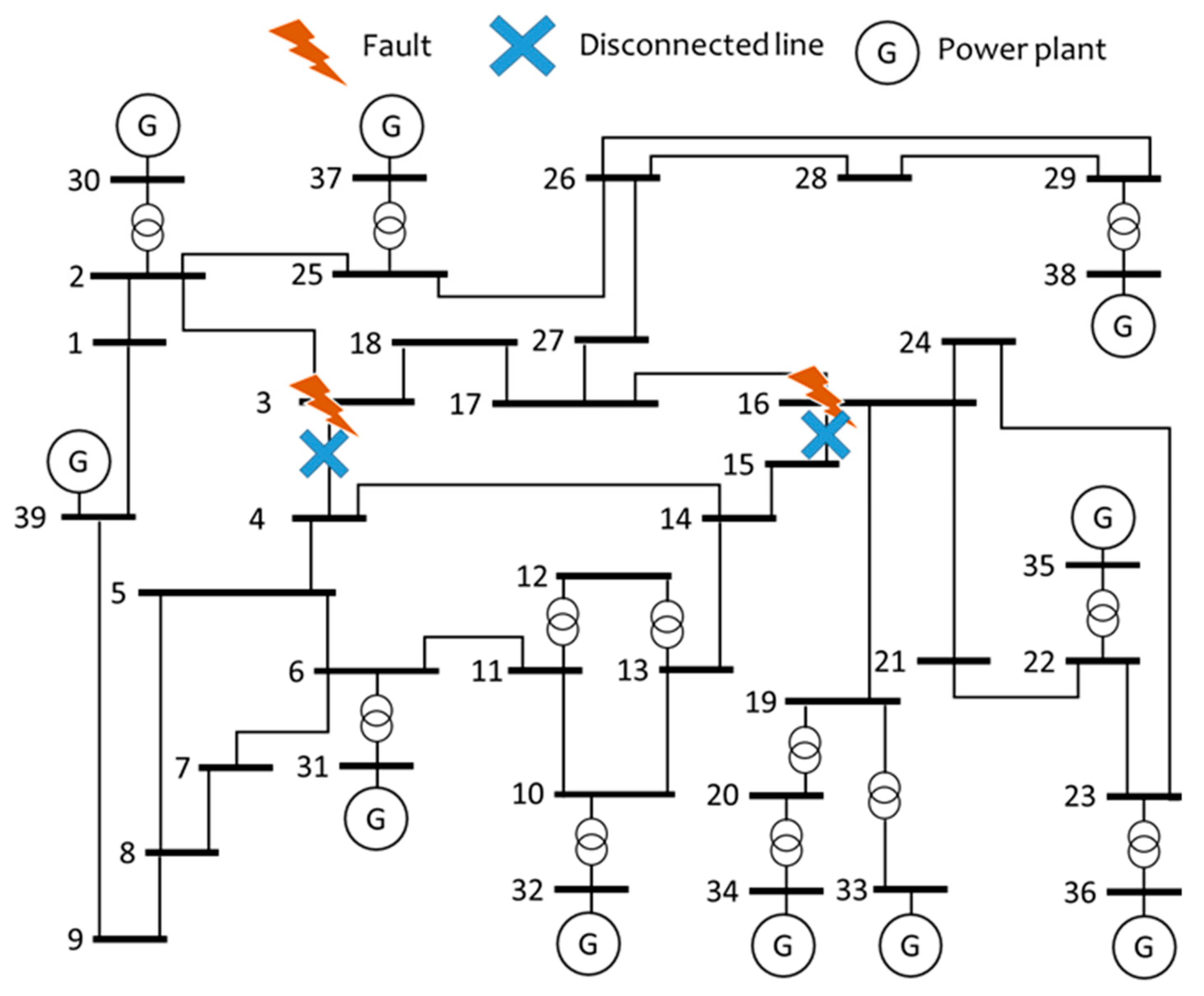
The study is applied to the IEEE 39 Bus New England benchmark test system, represented in Figure 2. The system data can be found in [23]. Two different contingencies have been analyzed, as shown in Figure 2:
- A three-phase short-circuit occurs in the transmission line connecting buses 15 and 16—adjacent to bus 16. The fault is cleared by opening the circuit breakers at the two ends of this line after 300 ms.
- A three-phase short-circuit occurs in the transmission line connecting buses 3 and 4—adjacent to bus 3. The fault is cleared by opening the circuit breakers at the two ends of this line after 300 ms.
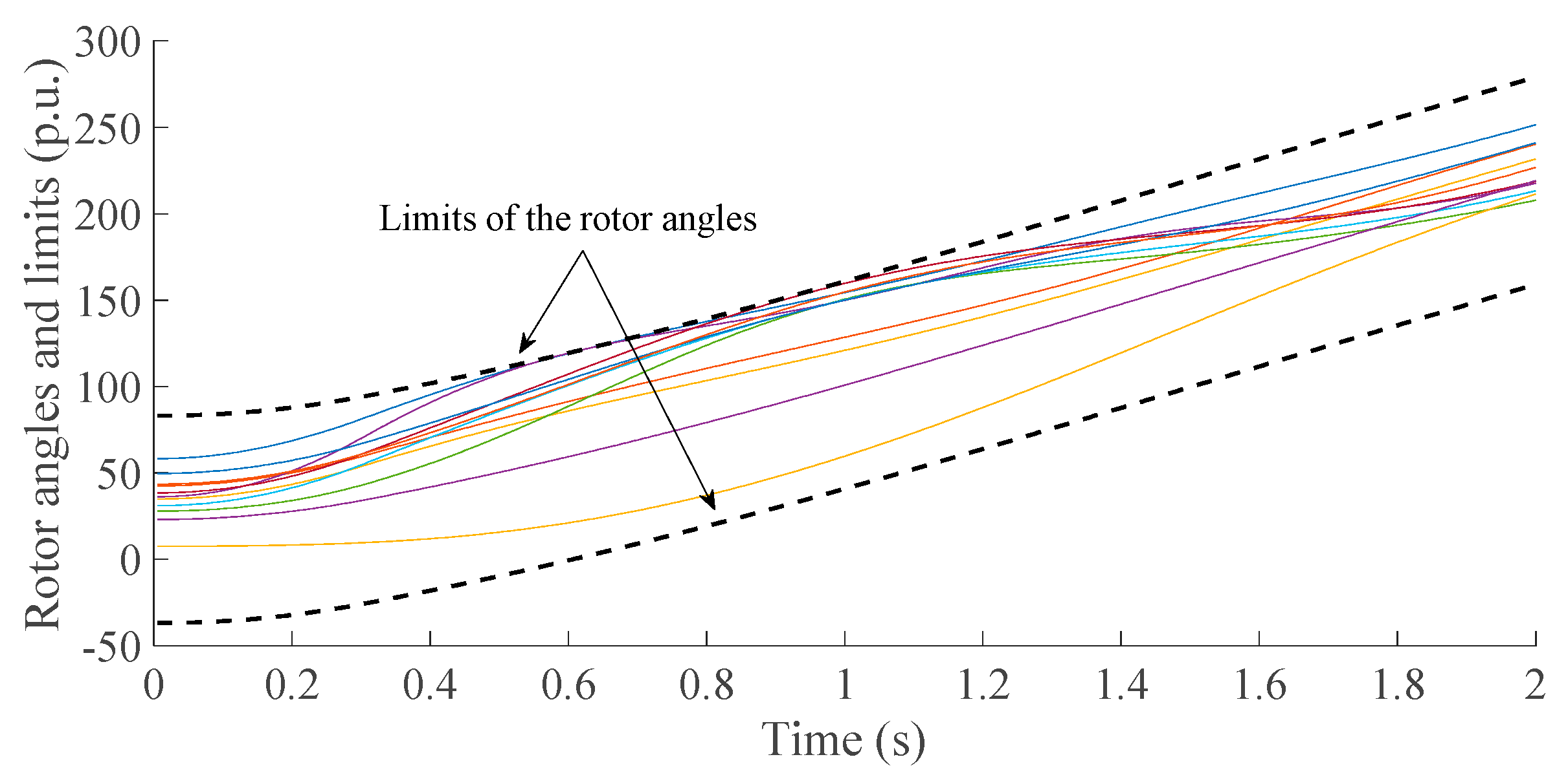
These faults have been selected because they pose a considerable risk to transient stability due, on the one hand, to their location in the bulk of the transmission system and, on the other hand, to the fact that the loss of the line after the clearance of the fault significantly weakens the system. In all the studied cases the rotor angle deviation at one or more synchronous generators reaches its limits, which means that the dynamic constraints affect the optimal dispatch. In other words, the solution provided by a classical OPF is not transiently stable and the TSCOPF modifies the dispatch to ensure that the solution is stable. Thus, in the studied cases the production cost of the dispatch provided by the TSCOPF is always higher than the cost of the dispatch provided by a classical OPF. As an example, Figure 3 shows the rotor angles of all synchronous generators in one of the solved TSCOPF models; it can be seen that the upper angle constraint is reached at approximately t = 0.6 s.
The simulations in this paper have been performed using the IPOPT library on a personal computer equipped with a 3.40 GHz processor. The results obtained by a version of the proposed TSCOPF model that implemented a trapezoidal rule have been verified using dynamic simulations in PSSE [24].
4. Results and Discussion
4.1. Comparison between Numerical Integration Methods
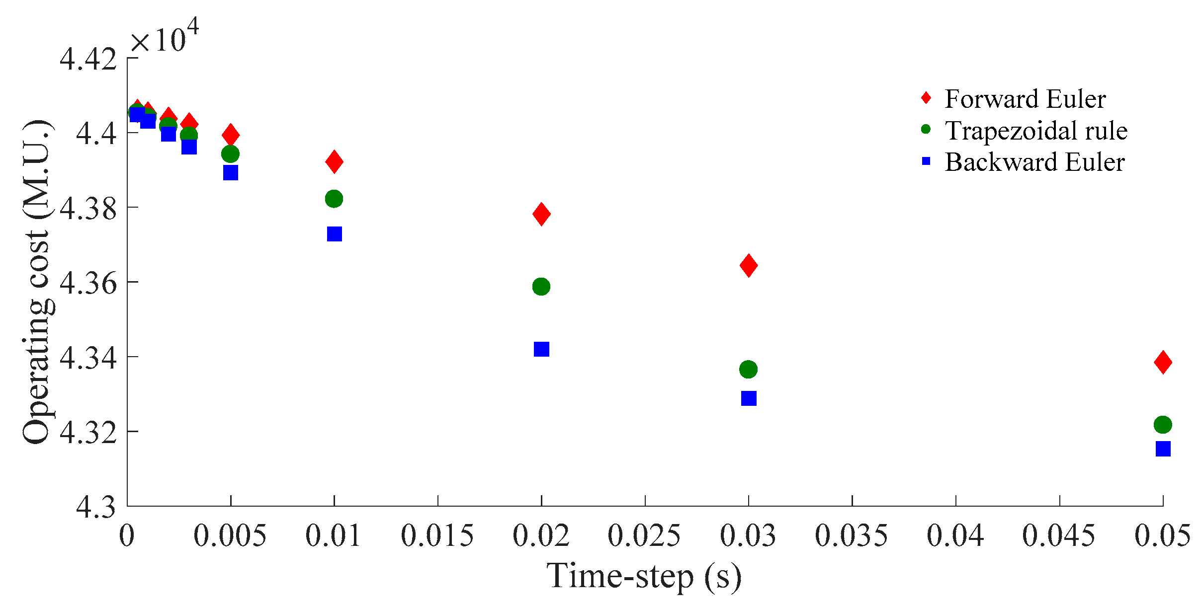
This section presents the influence of different integration methods on the solution of the TSCOPF model. Figure 4 shows the optimal production cost (i.e., the value of the objective function) calculated by the solution of the TSCOPF model when a short-circuit is applied at bus 16. The different values correspond to the three discretization methods implemented and several integration time steps. The study considers a time-horizon representation of 2 s after the fault.
It can be seen from Figure 4 that all three methods provide the same result when the integration step is small enough, while large integration steps produce different results depending on the integration method. To provide a term of comparison, a typical time step used in commercial power system simulators is one half of a cycle, this is 0.0083 s at 60 Hz and 0.01 s at 50 Hz. As can be seen, the forward Euler method is the least affected by the choice of integration step and the one that provides the most accurate solution in terms of the objective function. The largest errors are obtained with the backward Euler method, while the trapezoidal rule (the most commonly used method in TSCOPF studies) is located between the two variants of the Euler method.
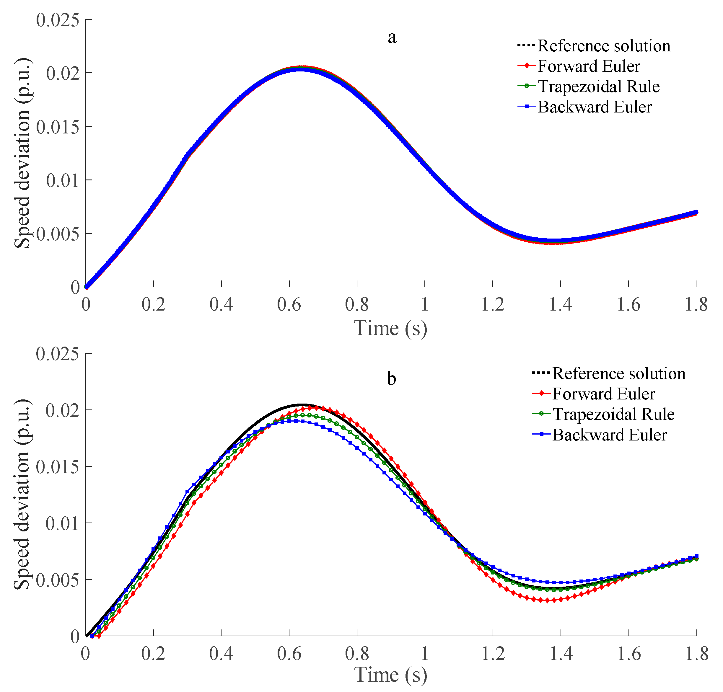
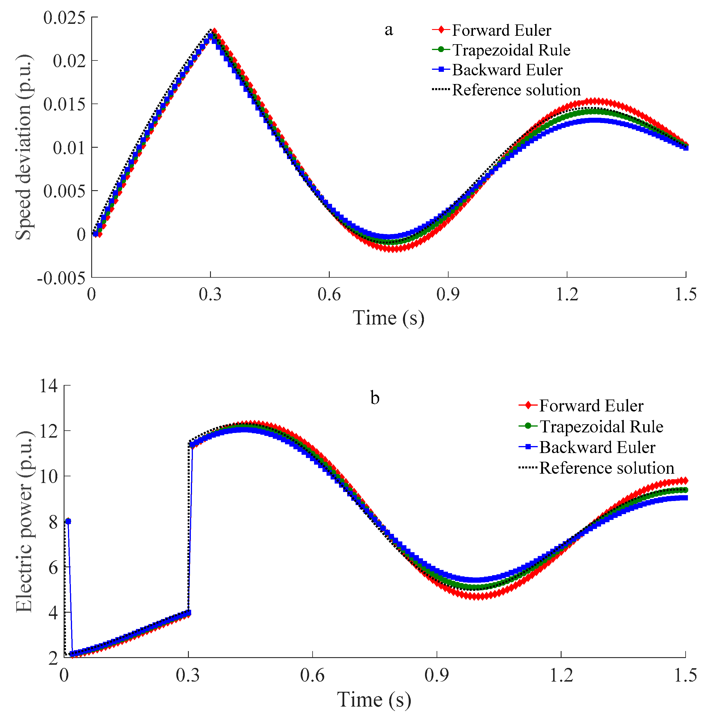
The results in Figure 4 may be explained by the trajectories of the rotor speed deviations given by the solution of the TSCOPF model when using each method. Figure 5 shows the speed deviation of the power plant at bus 33 using two integration time steps, 0.002 and 0.02 s. It can be seen in Figure 5a that for small integration steps the trajectories are similar. The common solution in Figure 5a, when the step size approaches zero, is taken as the reference solution in Figure 5b, which shows the electromechanical oscillations obtained with a larger integration time step by the three implemented methods. Figure 5b shows that the solution obtained by the backward Euler method is significantly damped compared to the reference solution. The oscillation obtained using the trapezoidal rule is damped, as well, but to a lesser degree. As a result, the solutions provided by the backward Euler method and the trapezoidal rule are more stable than the reference solution and their operating costs are lower, as shown in Figure 4. On the other hand, it can be seen that the forward Euler method augments the electromechanical oscillations with respect to the reference solution, which implies a more conservative solution.
Figure 6 shows two more examples corresponding to a short circuit at bus 3. Figure 6a represents the rotor speed deviation at the generator at bus 30, and Figure 6b the active power produced by the generator at bus 30. In both cases, it can be seen that the results are qualitatively similar to those discussed in Figure 5; as the integration time step increases the solution provided by the backward Euler method and the trapezoidal rule is damped compared to the reference solution, as opposed to the forward Euler method.
The backward Euler method and the trapezoidal rule are A-stable. This makes both methods well suited for numerical integration of stiff systems in general, and power system in particular [16,19]. Thus, it must be stressed that integration methods that are numerically stable can produce dispatches that are transiently unstable in the real world because they tend to damp electromechanical oscillations with respect to the real trajectories when large integration time steps are used.
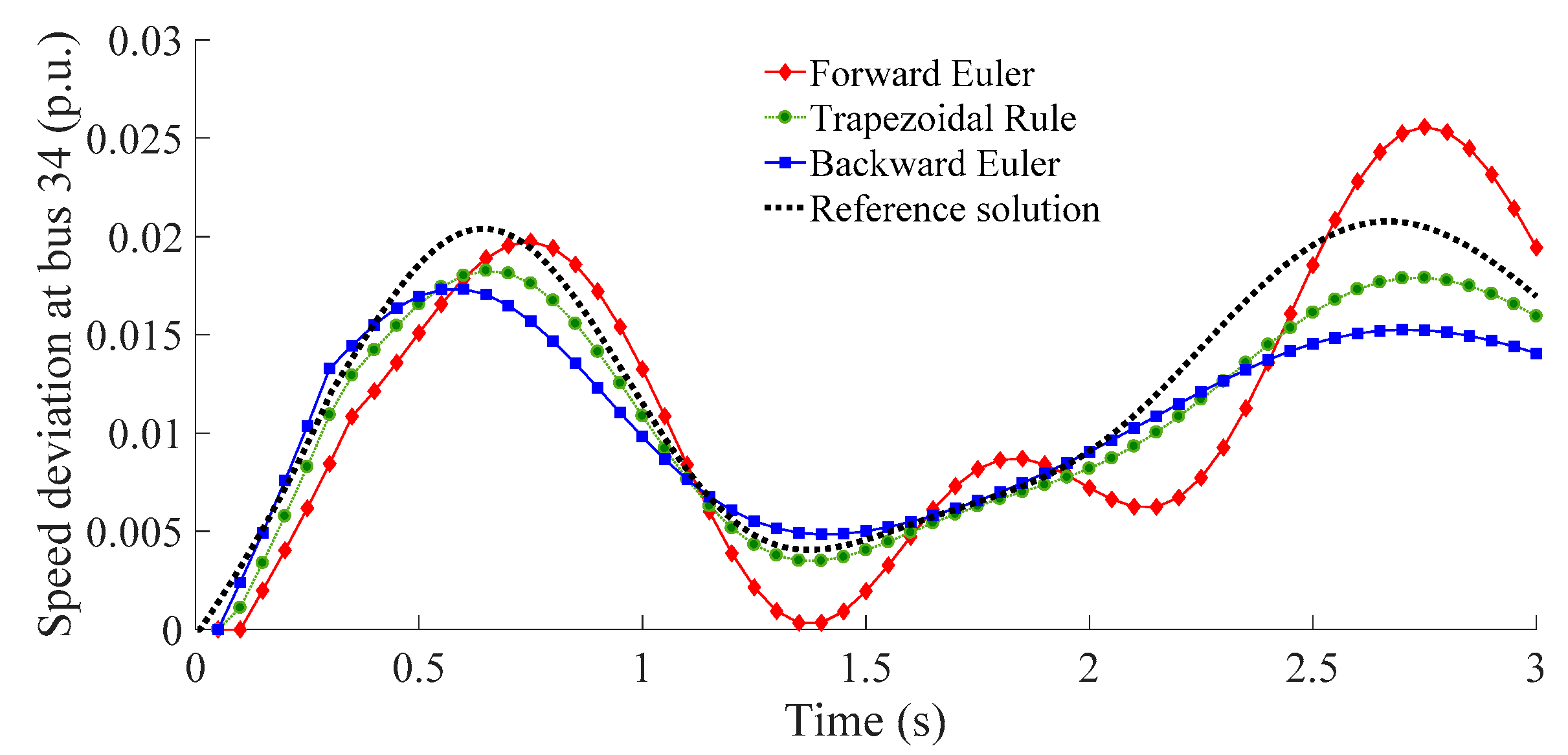
Regarding the numerical convergence of the solution, it must be observed that it has not been possible to obtain solutions of the TSCOPF model with the forward Euler method and time steps longer than 0.05 s. Figure 7 shows the rotor speed deviation at the synchronous generator connected to bus 34 when a short circuit is applied at bus 16 and the integration step is as large as 0.05 s. The trajectory obtained by the forward Euler method differs largely from the other two methods and the reference. This can be explained by the poor numerical stability of the forward Euler method.
Regarding the computation time, Table 2 presents the convergence times for the three cases of study in Figure 4. It can be seen that the computation time increases rapidly that as the integration step decreases. For example, as the integration step is divided by 10 from 0.01 to 0.001, the computation time is multiplied by 34 (forward Euler), by 44 (trapezoidal rule) and by 39 (backward Euler). The reason is that reducing the integration step increases the number of equality constraints in the optimization model. When large integration steps are used the convergence times are similar in the three methods. As the integration step decreases, and although the results vary depending on the specific case, it is observed that the optimization model applying the trapezoidal rule is solved with the shortest computational time. It is remarkable that the increase in computation time is not proportional to the number of equations or variables, as can be seen in the rows showing Time/Equations and Time/Variables. According to the results in this section it can be concluded that in terms of accuracy and calculation times, an integration time step of 0.01–0.02 s seems to be the optimal choice.
4.2. Simulation of Other Disturbances
This section shows the results of applying the TSCOPF algorithm to other types of contingencies using the different integration methods presented in Section 4.1. Three different types of contingencies are studied: (1) the power outage of a generator; (2) the loss of a load; and (3) the loss of a line. Three of the most severe cases are presented here:
- The power outage of power plant connected to bus 30 which is injecting 800 MW to the grid
- The loss of the load connected to bus 20 which is the largest of the system and consumes 680 MW.
- The loss of the line connecting buses 2 and 3.
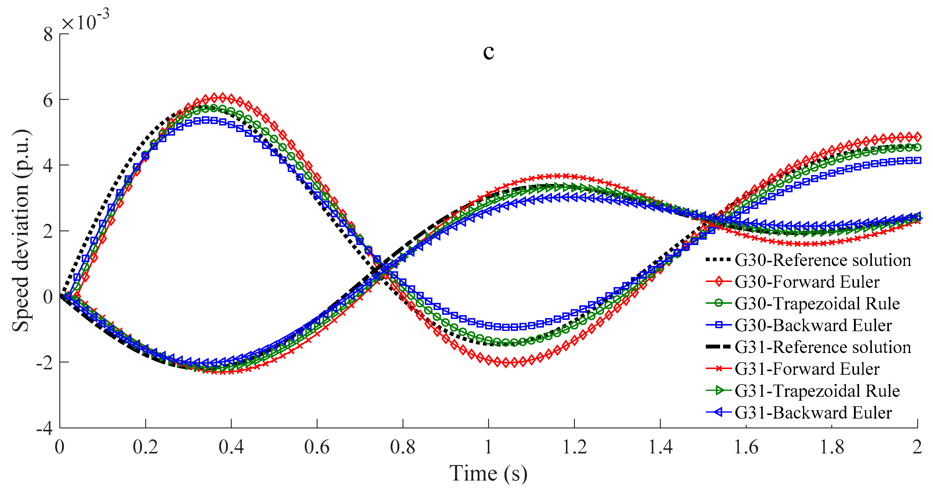
In contrast to the three-phase short-circuits presented previously these contingencies are not critical, which means that the operational costs given by the TSCOPF is the same obtained with an OPF. Figure 8 illustrates the speed deviation of different power plants when the described contingencies occur. Figure 8a shows the rotor speed deviation of power plants connected to buses 37 and 38 after a sudden disconnection of the power plant connected to bus 30. It can be observed how the speed of the machines decreases as they assume the generation of the disconnected power plant. It is remarkable how the curves obtained using the different integration methods follow the same tendency as those presented in Section 4.1. The forward Euler method presents the most conservative solution because it maintains the size of the oscillations. On the other hand, the trapezoidal rule and, to a higher degree, the backward Euler method damp the oscillations with respect to the reference solution. Figure 8b shows the rotor speed deviation of power plants connected to buses 34 and 36 when the load connected to bus 20 is shed.
In this scenario, the rotor speed of synchronous machines increases as they transform the demand of the disconnected load into kinetic energy. Again, the result of the curves obtained by the different integration methods follows the same tendency. Finally, Figure 8c shows the rotor speed deviation of power plants connected to buses 30 and 31 when the line connecting buses 2 and 3 is lost. Similar conclusions can be obtained here with respect to the different integration methods.
4.3. Generalized Theta Method
The Theta method represents alternatively the forward Euler method, when Theta = 1, the Trapezoidal Rule, when Theta = 0.5, and the backward Euler method, when Theta = 0 [17]. The generalized Theta method makes it possible to extend the range of application of this notation by assigning to Theta any other number between 0 and 1 in Equations (14)–(17).
Figure 9 shows the generation costs obtained when different values of Theta are used in the case of a short circuit at bus 16 and various time steps. A similar result is obtained with all the Theta values for short integration time steps However, as the integration step increases, the result obtained for the same case increases as the Theta value grows. These results are consistent with those shown in the previous section: the forward Euler method provides a more conservative solution, and therefore a slightly higher generation cost. As shown in Figure 9, the relation between the value of Theta and the generation cost when the generalized Theta method is applied is essentially linear.
Figure 10 shows the computation time needed to solve the cases in Figure 9. Similar convergence times are obtained using large integration time steps since the size of the optimization problem is small. However, it can be observed that the computation time tends to increase with Theta = 0 and with Theta = 1 when the time step is short. These are the cases corresponding to the forward and backward Euler methods, which are the cases in which the state variables appear at just one discretization point in the discretized differential Equations (14)–(17). According to Figure 10, when the computation time is an issue it is advisable to avoid these methods.
4.4. Comparison with RK2 and RK4 Runge-Kutta Methods
This section analyzes the performance of the second and fourth order Runge-Kutta methods (RK2 and RK4). These methods are rarely used in TSCOPF studies because implicit methods are usually preferred due to their numerical stability. The interest of Runge-Kutta methods lies in that they are widely used to solve differential-algebraic equation systems in general, and power system dynamic models in transient stability software programs in particular.
The implementation of the RK2 and RK4 methods involves the introduction of several intermediate variables and constraints to represent the differential equations (2 constraints per differential equation in the case of RK2 and 4 in the case of RK4). This has the unwanted effect of increasing the already large size of the optimization model, which is one of the main drawbacks of TSCOPF studies in real systems applications.
The 4th order d-q generator model is represented by four differential equations [7]. Constraints (30)–(34) result from the application of the RK4 method to the differential equation that calculates the transient voltage in the d-axis and serve as an example of the implementation of the RK4 method in the optimization model. Therefore, constraints (30)–(34) replace constraint (15) in the original optimization model (1)–(9), (14)–(29). As can be seen, five different constraints and four intermediate variables (k1D, k2D, k3D and k4D) must be added for each differential equation. Similarly, constraints (14), (16) and (17) must be substituted with the corresponding RK4. In the case of implementing the RK2 method, each differential equation requires three equations and two intermediate variables in the optimization model:
Table 3 shows the results obtained when applying the different algorithms to a short circuit at bus 16 and an integration time step of 0.002 s. It can be seen that the size of the model in terms of number of variables and number of constraints increases significantly with the order of the Runge-Kutta method. The computational time needed to solve the model increases too, although the number of iterations remains relatively small.
In the studied cases, it has not been possible to solve the model using the Runge-Kutta algorithms with integration time steps larger than 0.005 s or shorter than 0.0005 s. On the one hand, the size of the optimization model prevents the use of small integration time steps. On the other hand, numerical convergence issues prevent the use of large integration time steps. It can be concluded that in the studied cases the combined effect of the size of the model and numerical stability narrows the applicability of the Runge-Kutta methods to a point that can make them unfeasible for TSCOPF studies.
4.5. Effect of the Use of a Variable Integration Time Step
This section proposes the use of a variable integration step to reduce the convergence time. The implementation is carried out as follows: (1) A short time step is applied during the first second, to account for the severe transients produced during the fault and after the clearance of the fault; and (2) from that moment on a larger integration step is applied. This approach is adequate, since as shown in Figure 3, the generators reach the transient stability limit at approximately 0.6 s after the fault, before shifting to the longer time step.
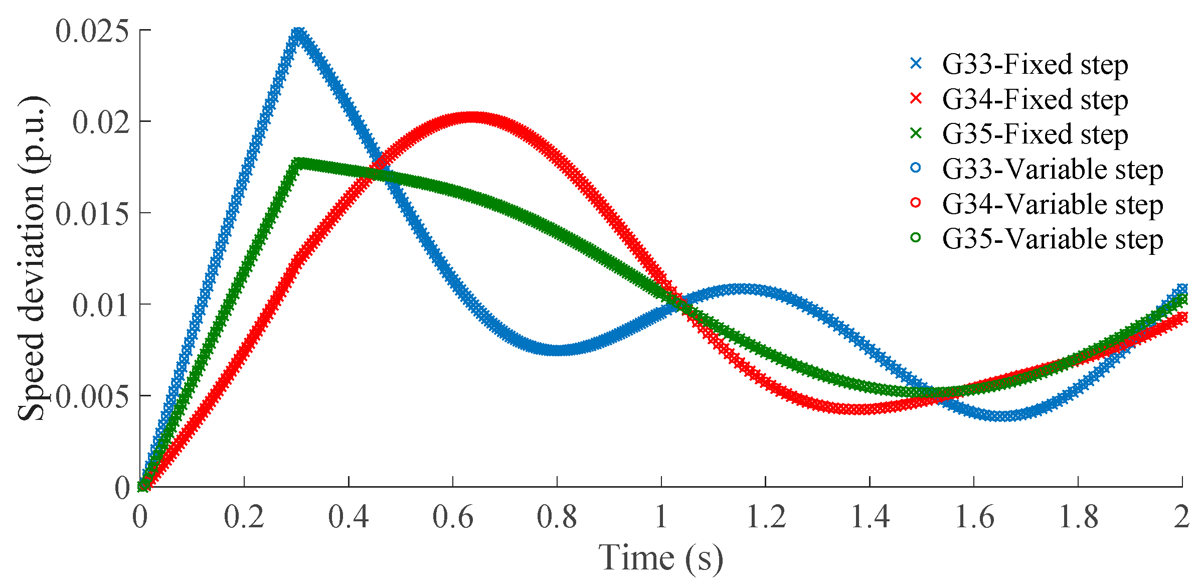
Table 4 shows the results obtained with and without a variable time step when a short-circuit is applied at bus 3. The first case uses a fixed time integration step of 0.005 s. The second case applies an integration time step of 0.005 s during the first second, and a step of 0.01 s from then on. It can be seen in Table 4 that the application of a variable integration time step reduces the size of the optimization problem: the number of equations is decreased by 24.97% and the number of variables by 24.99%. However, the impact on the computation time is more significant, reducing it by 79.48% with the forward Euler method, by 58.10% with the trapezoidal rule, and by 74.31% with the backward Euler method. The high impact on the reduction in terms of convergence times is due to the large nonlinearity between the computation time and the step size, as shown in Table 2.
Regarding the accuracy of the results, Figure 11 compares the rotor speed deviation of all the synchronous generators when using the trapezoidal rule with fixed and variable integration time steps as described above. It can be seen that the results are almost identical.
These results show that the use of a variable integration step in the TSCOPF model achieves a considerable reduction in computation times while maintaining the accuracy of the results. The results obtained for other contingencies have been qualitatively similar to those presented here.
5. Conclusions
The performance of several numerical integration methods in a transient stability constrained optimal power flow based on simultaneous discretization has been analyzed. The trapezoidal rule, the backward Euler method and the forward Euler method have been found to be practical alternatives, with these differences:
- In terms of convergence, no problems were observed in the studied cases for time steps shorter than 0.05 s. However, the forward Euler method provides results that differ significantly from the reference solution when the integration time step is 0.05 s and fails to converge if larger integration steps are used. As expected, the numerical stability of the forward Euler method is known to be poor compared to implicit integration methods. Although the forward Euler method is viable in the studied case, in other cases numerical stability could be a problem depending on the stiffness of the set of differential-algebraic equations representing the dynamics of the power system.
- In terms of the numerical solution, it has been found that the backward Euler method and, in less degree, the trapezoidal rule, tend to damp the electromechanical oscillations. This effect increases with the length of the integration time step and can lead to dispatches that produce unstable cases in the real world. Operators assessing the stability of a system should be aware of this effect, and perhaps compensate it by introducing a security margin in the dynamic constraints of the optimization model.
- In terms of the speed of convergence, the trapezoidal rule or, more exactly, any generalized Theta method with values of Theta larger than zero and smaller than one, has been found to be faster than the forward and the backward Euler methods.
In sum, all three methods have been found to be viable and an integration time step length of 0.01 s has provided accurate solutions and reasonable convergence times. Although in the studied cases the trapezoidal rule represents a good compromise between numerical stability, convergence speed and accuracy of the solution, the forward Euler method provides more conservative results. It is therefore advisable to keep the Theta formulation in the optimization model to be able to explore both methods depending on the specific case they are applied to.
Finally, the use of a variable integration time step has proved to be a valid technique to reduce the number of equations and variables of the optimization model and, substantially, convergence times. Reductions of up to almost 80% have been obtained and no problems of convergence or errors in the solution have been observed when using adequate variable integration steps.
Author Contributions
Conceptualization, F.A., E.D.C. and P.L.; Methodology, F.A.; Software, F.A.; Supervision, E.D.C., P.L. and Z.L.; Writing—review & editing, F.A., E.D.C., P.L. and Z.L.
Funding
This research received no external funding.
Conflicts of Interest
The authors declare no conflict of interest.
Nomenclature
| Abbreviations | |
| COI | Center of Inertia |
| GAMS | General Algebraic Modeling System |
| OPF | Optimal Power Flow |
| PF | Pre-Fault |
| PSSE | Power System Simulator for Engineering |
| RK2 | 2nd order Runge-Kutta method. |
| RK4 | 4th order Runge-Kutta method. |
| TD | Time Domain |
| TSCOPF | Transient Stability Constrained Optimal Power Flow. |
| Indices and sets | |
| i,j | Indices for nodes. |
| t | Indices for time periods. |
| Set of buses of the power system. | |
| Set of the synchronous generation units. | |
| Set of loads | |
| Set of the time periods corresponding to the pre-fault, fault and post fault stages. | |
| Set of the time periods corresponding to the fault and post fault stages. | |
| Parameters | |
| Fuel cost coefficients of the power plants. | |
| Active power coefficients of the ZIP load model. | |
| Reactive power coefficients of the ZIP load model. | |
| Damping coefficient of the power plant [p.u.]. | |
| Limits of the field voltage of the synchronous generator [p.u.]. | |
| Inertia constant of the power plant [s]. | |
| Upper limit of the current in lines and transformers. [p.u.]. | |
| Active and reactive nominal load [p.u.]. | |
| Active power limits of the generator [p.u.]. | |
| Reactive power limits of the generator [p.u.]. | |
| Armature resistance [p.u.]. | |
| Generator transient time constants[s]. | |
| Parameter that defines the numerical integration method. | |
| Limits of the bus voltage [p.u.]. | |
| Synchronous reactances of the power plant [p.u.]. | |
| Transient synchronous reactances of the power plant [p.u.]. | |
| Absolut value of the element (i,j) of the bus admittance matrix [p.u.]. | |
| Integration time step [s]. | |
| Phase of the element (i,j) of the bus admittance matrix [p.u.]. | |
| Frequency reference | |
| Limit of the rotor angle deviation [rad]. | |
| Variables | |
| Internal transient voltages of the synchronous generator [p.u.]. | |
| Field voltage of the synchronous generator [p.u.]. | |
| Output current d-q components of the synchronous generator [p.u.]. | |
| Current between nodes (i,j) [p.u.]. | |
| Intermediate variables for the calculation of the transient voltage in the d-axis when using the RK4 method | |
| Electrical power in the rotor of the synchronous generator [p.u.] | |
| Active and reactive power output of the synchronous generator [p.u.]. | |
| Active and reactive load | |
| Mechanical power input of the power plant [p.u.]. | |
| Bus voltage magnitude [p.u.]. | |
| Speed deviation of the synchronous generator [rad/s]. | |
| Phase of the bus voltage [rad]. | |
| Rotor angle [rad]. | |
| Rotor angle of the center of inertia [rad]. |
References
- Abhyankar, S.; Geng, G.; Anitescu, M.; Wang, X.; Dinavahi, V. Solution techniques for transient stability-constrained optimal power flow—Part I. IET Gener. Transm. Distrib. 2017, 11, 3177–3185. [Google Scholar] [CrossRef]
- Geng, G.; Abhyankar, S.; Wang, X.; Dinavahi, V. Solution techniques for transient stability-constrained optimal power flow—Part II. IET Gener. Transm. Distrib. 2017, 11, 3186–3193. [Google Scholar] [CrossRef]
- Capitanescu, F.; Martinez Ramos, J.L.; Panciatici, P.; Kirschen, D.; Marano Marcolini, A.; Platbrood, L.; Wehenkel, L. State-of-the-art, challenges, and future trends in security constrained optimal power flow. Electr. Power Syst. Res. 2011, 81, 1731–1741. [Google Scholar] [CrossRef] [Green Version]
- Arredondo, F.; Castronuovo, E.; Ledesma, P.; Leonowicz, Z. Comparative Implementation of Numerical Integration Methods for Transient Stability Constrained Optimal Power Flow. In Proceedings of the 2018 IEEE International Conference on Environment and Electrical Engineering and 2018 IEEE Industrial and Commercial Power Systems Europe (EEEIC/I CPS Europe), Palermo, Italy, 12–15 June 2018; pp. 1–6. [Google Scholar]
- Sanchez-Gasca, J.J.; D’Aquila, R.; Paserba, J.J.; Price, W.W.; Klapper, D.B.; Hu, I.-P. Extended-term dynamic simulation using variable time step integration. IEEE Comput. Appl. Power 1993, 6, 23–28. [Google Scholar] [CrossRef]
- Gao, Y.; Wang, J.; Xiao, T.; Jiang, D. A Transient Stability Numerical Integration Algorithm for Variable Step Sizes Based on Virtual Input. Energies 2017, 10, 1736. [Google Scholar] [CrossRef]
- Sauer, P.W.; Pai, M.A. Power System Dynamics and Stability; Prentice Hall: Upper Saddle River, NJ, USA, 1998; Volume 51. [Google Scholar]
- Gan, D.; Thomas, R.J.; Zimmerman, R.D. Stability-constrained optimal power flow. IEEE Trans. Power Syst. 2000, 15, 535–540. [Google Scholar] [CrossRef] [Green Version]
- Ledesma, P.; Arredondo, F.; Castronuovo, E.D. Optimal Curtailment of Non-Synchronous Renewable Generation on the Island of Tenerife Considering Steady State and Transient Stability Constraints. Energies 2017, 10, 1926. [Google Scholar] [CrossRef]
- Zarate-Minano, R.; Van Cutsem, T.; Milano, F.; Conejo, A.J. Securing Transient Stability Using Time-Domain Simulations Within an Optimal Power Flow. IEEE Trans. Power Syst. 2010, 25, 243–253. [Google Scholar] [CrossRef] [Green Version]
- Jiang, Q.; Huang, Z. An Enhanced Numerical Discretization Method for Transient Stability Constrained Optimal Power Flow. IEEE Trans. Power Syst. 2010, 25, 1790–1797. [Google Scholar] [CrossRef]
- Arredondo, F.; Ledesma, P.; Castronuovo, E.D. Optimization of the operation of a flywheel to support stability and reduce generation costs using a Multi-Contingency TSCOPF with nonlinear loads. Int. J. Electr. Power Energy Syst. 2019, 104, 69–77. [Google Scholar] [CrossRef]
- Weckesser, T.; Jóhannsson, H.; Østergaard, J. Impact of model detail of synchronous machines on real-time transient stability assessment. In Proceedings of the 2013 IREP Symposium Bulk Power System Dynamics and Control—IX Optimization, Security and Control of the Emerging Power Grid, Rethymno, Greece, 25–30 August 2013; pp. 1–9. [Google Scholar]
- Tu, X.; Dessaint, L.; Kamwa, I. A global approach to transient stability constrained optimal power flow using a machine detailed model. Can. J. Electr. Comput. Eng. 2013, 36, 32–41. [Google Scholar] [CrossRef]
- Eberly, D. Stability Analysis for Systems of Differential Equations; 2008. Available online: https://www.geometrictools.com/Documentation/StabilityAnalysis.pdf (accessed on 8 December 2018).
- Milano, F. Power System Modelling and Scripting; Springer: Berlin, Germany, 2010; ISBN 978-3-642-13669-6. [Google Scholar]
- Faragó, I. Convergence and stability constant of the theta-method. Appl. Math. 2013, 2013, 42–51. [Google Scholar]
- Milano, F. An Open Source Power System Analysis Toolbox. IEEE Trans. Power Syst. 2005, 20, 1199–1206. [Google Scholar] [CrossRef]
- Kundur, P.; Balu, N.J.; Lauby, M.G. Power System Stability and Control; McGraw-hill: New York, NY, USA, 1994. [Google Scholar]
- GAMS—Cutting Edge Modeling. Available online: https://www.gams.com/ (accessed on 6 March 2018).
- IPOPT. Available online: https://projects.coin-or.org/Ipopt (accessed on 6 March 2018).
- IPOPT and IPOPTH. Available online: http://citeseerx.ist.psu.edu/viewdoc/download?doi=10.1.1.589.5002&rep=rep1&type=pdf (accessed on 28 March 2018).
- Power Flow Cases—Illinois Center for a Smarter Electric Grid (ICSEG). Available online: http://icseg.iti.illinois.edu/power-cases/ (accessed on 28 March 2018).
- Ledesma, P.; Calle, I.A.; Castronuovo, E.D.; Arredondo, F. Multi-contingency TSCOPF based on full-system simulation. IET Gener. Transm. Distrib. 2017, 11, 64–72. [Google Scholar] [CrossRef] [Green Version]
Figure 1.
Software implementation for TSCOPF.

Figure 2.
IEEE 39 Bus New England benchmark system with fault locations corresponding to the study in Section 4.
Figure 2.
IEEE 39 Bus New England benchmark system with fault locations corresponding to the study in Section 4.

Figure 3.
Synchronous generator rotor angles as provided by the solution of the TSCOPF when a short circuit is applied at bus 16.
Figure 3.
Synchronous generator rotor angles as provided by the solution of the TSCOPF when a short circuit is applied at bus 16.

Figure 4.
TSCOPF result for the short-circuit at bus 16, obtained using different numerical integration methods and time steps.
Figure 4.
TSCOPF result for the short-circuit at bus 16, obtained using different numerical integration methods and time steps.

Figure 5.
Rotor speed deviation at the generator at bus 33 when a short circuit is applied at bus 16. (a) with an integration time step of 0.002 s (b) with an integration time step of 0.02.
Figure 5.
Rotor speed deviation at the generator at bus 33 when a short circuit is applied at bus 16. (a) with an integration time step of 0.002 s (b) with an integration time step of 0.02.

Figure 6.
Two variables when a short circuit is applied at bus 3 and the integration time step is 0.01 s: (a) Rotor speed deviation at the generator at bus 30 (b) Electric power output at the generator at bus 30.
Figure 6.
Two variables when a short circuit is applied at bus 3 and the integration time step is 0.01 s: (a) Rotor speed deviation at the generator at bus 30 (b) Electric power output at the generator at bus 30.

Figure 7.
Rotor speed deviation at the generator at bus 34 when a short circuit at bus 16 and a integration time step of 0.05 s.
Figure 7.
Rotor speed deviation at the generator at bus 34 when a short circuit at bus 16 and a integration time step of 0.05 s.

Figure 8.
Rotor speed deviation of generators. (a) Generators 37 and 38 when a power outage of generator connected to bus 30. (b) Generators 34 and 36 when the loss of the load connected to bus 20. (c) Generators 30 and 31 when the loss of line 2–3.
Figure 8.
Rotor speed deviation of generators. (a) Generators 37 and 38 when a power outage of generator connected to bus 30. (b) Generators 34 and 36 when the loss of the load connected to bus 20. (c) Generators 30 and 31 when the loss of line 2–3.


Figure 9.
Results of the TSCOPF depending on the value of Theta when a short circuit is applied at bus 16.
Figure 9.
Results of the TSCOPF depending on the value of Theta when a short circuit is applied at bus 16.

Figure 10.
Computation time depending on the value of Theta when a short circuit is applied at bus 16.
Figure 10.
Computation time depending on the value of Theta when a short circuit is applied at bus 16.

Figure 11.
Rotor speed deviation of generators connected to nodes 33, 34 and 35 as provided by the solution of the TSCOPF when a short circuit at bus 16 using a fixed and variable integration time step.
Figure 11.
Rotor speed deviation of generators connected to nodes 33, 34 and 35 as provided by the solution of the TSCOPF when a short circuit at bus 16 using a fixed and variable integration time step.


Table 1.
Summary of the constraints of the optimization problem.
| Network and load modeling | Equality constraints | PF | TD |
| Power flow Equations (2) and (3) | Χ | Χ | |
| Angle reference (4) | Χ | - | |
| Load Equations (6) and (7) | Χ | Χ | |
| Currents in branches and transformers (8) | Χ | - | |
| Inequality constraints | PF | TD | |
| Voltage limits at buses (5) | Χ | - | |
| Active and reactive power generation limits (5) | Χ | - | |
| Maximum currents through branches and transformers (9) | Χ | - | |
| Power plant modeling | Equality constraints | PF | TD |
| Discretized differential equations of power plants (14)–(17) | - | Χ | |
| Initialization of the differential Equations (18)–(21) | Χ | - | |
| Power plant static Equations (22)–(26) | Χ | Χ | |
| Inequality constraints | PF | TD | |
| Field voltage limits (27) | Χ | Χ | |
| Stability Limits | Equality constraints | PF | TD |
| Calculation of the center of inertia (28) | Χ | Χ | |
| Inequality constraints | PF | TD | |
| Rotor angle deviation limits (29) | Χ | Χ |
Table 2.
Time of convergence of the TSCOPF for the studied numerical integration methods and different integration time steps.
Table 2.
Time of convergence of the TSCOPF for the studied numerical integration methods and different integration time steps.
| 0.0005 | 0.001 | 0.002 | 0.003 | 0.005 | 0.01 | 0.02 | 0.05 | |
|---|---|---|---|---|---|---|---|---|
| Equations | 680,071 | 340,071 | 170,071 | 113,291 | 68,071 | 34,071 | 17,071 | 6871 |
| Variables | 600,030 | 300,030 | 150,030 | 60,030 | 30,030 | 15,030 | 9930 | 6030 |
| Forward Euler | ||||||||
| Time (s) | 4211 | 796 | 394 | 188 | 157.6 | 23.48 | 9.95 | 2.84 |
| Time/Equations | 6.2 × 10⁻³ | 2.3 × 10⁻³ | 2.3 × 10⁻³ | 1.7 × 10⁻³ | 2.3 × 10⁻³ | 7 × 10⁻⁴ | 6 × 10⁻⁴ | 4 × 10⁻⁴ |
| Time/Variables | 7 × 10⁻³ | 2.7 × 10⁻³ | 2.6 × 10⁻³ | 1.9 × 10⁻³ | 2.6 × 10⁻³ | 8 × 10⁻⁴ | 7 × 10⁻⁴ | 5 × 10⁻⁴ |
| Trapezoidal Rule | ||||||||
| Time (s) | 3799 | 774 | 184 | 176 | 69.3 | 17.7 | 7.85 | 2.83 |
| Time/Equations | 5.6 × 10⁻³ | 2.3 × 10⁻³ | 1.1 × 10⁻³ | 1.6 × 10⁻³ | 1 × 10⁻³ | 5 × 10⁻⁴ | 4.6 × 10⁻⁴ | 4 × 10⁻⁴ |
| Time/Variables | 6.3 × 10⁻³ | 2.6 × 10⁻³ | 1.2 × 10⁻³ | 1.8 × 10⁻³ | 1.2 × 10⁻³ | 5.9 × 10⁻⁴ | 5.2 × 10⁻⁴ | 4.7 × 10⁻⁴ |
| Backward Euler | ||||||||
| Time (s) | 5739 | 1055 | 537 | 289 | 116 | 18 | 7.97 | 2.94 |
| Time/Equations | 8.4 × 10⁻³ | 3.1 × 10⁻³ | 3.2 × 10⁻³ | 2.6 × 10⁻³ | 1.7 × 10⁻³ | 5.3 × 10⁻⁴ | 4.7 × 10⁻⁴ | 4.3 × 10⁻⁴ |
| Time/Variables | 9.6 × 10⁻³ | 3.5 × 10⁻³ | 3.6 × 10⁻³ | 2.9 × 10⁻³ | 1.9 × 10⁻³ | 6 × 10⁻⁴ | 5.3 × 10⁻⁴ | 4.9 × 10⁻⁴ |
Table 3.
Comparison of the common methods used in TSCOPF with the Runge Kutta methods.
| Method | Forward Euler | Trapezoidal Rule | Backward Euler | Runge Kutta 2 | Runge Kutta 4 |
|---|---|---|---|---|---|
| Number of variables | 150,030 | 150,030 | 150,030 | 459,950 | 619,870 |
| Number of constraints | 170,071 | 170,071 | 170,071 | 499,991 | 659,911 |
| Number of iterations | 50 | 49 | 56 | 55 | 54 |
| CPU time (s) | 404 | 347 | 451 | 1463 | 1438 |
Table 4.
Results of TSCOPF considering fixed and variable integration time step.
| Size | Fixed Step | Variable Step | ∆Size (%) | ||
| Equations | 68,071 | 51,071 | −24.97 | ||
| Variables | 60,030 | 45,030 | −24.99 | ||
| Method | Cost (M.U.) | Convergence (s) | Cost (M.U. 1) | Convergence (s) | ∆Convergence (%) |
| F. Euler | 43,993 | 157.708 | 43,960 | 32.359 | −79.48 |
| T. rule | 43,942 | 69.289 | 43,942 | 29.033 | −58.10 |
| B. Euler | 43,893 | 116.569 | 43,925 | 29.947 | −74.31 |
1 Monetary Units.
© 2019 by the authors. Licensee MDPI, Basel, Switzerland. This article is an open access article distributed under the terms and conditions of the Creative Commons Attribution (CC BY) license (http://creativecommons.org/licenses/by/4.0/).
Share and Cite
MDPI and ACS Style
Arredondo, F.; Castronuovo, E.D.; Ledesma, P.; Leonowicz, Z. Analysis of Numerical Methods to Include Dynamic Constraints in an Optimal Power Flow Model. Energies 2019, 12, 885. https://doi.org/10.3390/en12050885
AMA Style
Arredondo F, Castronuovo ED, Ledesma P, Leonowicz Z. Analysis of Numerical Methods to Include Dynamic Constraints in an Optimal Power Flow Model. Energies. 2019; 12(5):885. https://doi.org/10.3390/en12050885
Chicago/Turabian StyleArredondo, Francisco, Edgardo Daniel Castronuovo, Pablo Ledesma, and Zbigniew Leonowicz. 2019. "Analysis of Numerical Methods to Include Dynamic Constraints in an Optimal Power Flow Model" Energies 12, no. 5: 885. https://doi.org/10.3390/en12050885
Note that from the first issue of 2016, this journal uses article numbers instead of page numbers. See further details here.