A New Dynamic Model to Predict Transient and Steady State PV Temperatures Taking into Account the Environmental Conditions

Abstract

Photovoltaic (PV) cell and module temperature profiles, T_c and T_pv, respectively, developed under solar irradiance were predicted and measured both at transient and steady state conditions. The predicted and measured T_c or T_pv covered both a bare c-Si PV cell, by SOLARTEC, at laboratory conditions using a solar light simulator, as well as various c-Si and pc-Si modules (SM55, Bioenergy 195W, Energy Solutions 125W) operating in field conditions. The time constants, τ, of the T_c and T_pv profiles were determined by the proposed model and calculated using the experimentally obtained profiles for both the bare PV cell and PV modules. For model validation, the predicted steady state and transient temperature profiles were compared with experimental ones and also with those generated from other models. The effect of the ambient temperature, T_a, wind speed, v_w, and the solar irradiance, I_T, on the model performance, as well as of the mounting geometries, was investigated and incorporated in the prediction model. The predicted temperatures had the best matching to the measured ones in comparison to those from six other models. The model developed is applicable to any geographical site and environmental conditions.

1. Introduction

The photovoltaic (PV) temperature is a significant factor which affects the PV module performance through its effect on the PV cell electric characteristics, analytically presented in PV cell textbooks. Correspondingly, we speak about the PV module temperature, T_pv, and the PV cell temperature, T_c, which are equal provided the cells of the module are healthy and experience the same environmental conditions. It is of much interest to develop reliable models to predict T_pv, and the PV performance, through prediction of the power output P_m(t), when the module operates under any configuration and field conditions. Various mathematical expressions have been proposed and validated on their reliability to predict steady state T_pv [1,2,3,4,5,6,7,8,9], as to be discussed in detail later in this paper or transient T_pv profiles, [10,11,12,13,14] with good accuracy under any field conditions and for Building Integrated Photovoltaic (BIPV) configurations [15,16,17,18,19]. Those T_pv prediction models are grouped in: explicit models described in [1,2,3,4,5,6,7], usually physics based theoretical models which try to incorporate the environmental parameters, mainly, solar irradiance on the PV plane I_T, wind velocity v_w, wind direction, heat transfer from the PV to the environment, and radiation exchanges between PV and environment:

• Implicit models which use various algorithms and regression analysis to produce formulae to predict T_pv through quantities which depend on T_pv, as reviewed in [3,20].
• Theoretical based semi-empirical models, a mixture of Physics based processes elaborated on implicit functions, which through regression analysis incorporate the environmental conditions and develop expressions to predict T_pv including geometrical factors like PV module inclination, sun-tracking systems, BIPV [6,8,21].
• Approaches based on Artificial Neural Networks (ANN) [5,10,22].

An assessment of the T_pv prediction models discloses that those which have incorporated the radiation exchanges and the air flow regimes, where heat extraction off the modules is affected specifically, provide values closer to the measured ones [6,7,23,24,25]. A comparison among the models is necessary as to conclude on the conditions T_pv is predicted effectively and consistently. It is, therefore, necessary to compare T_pv models extensively to examine their validity in any PV configuration as the ones studied in [20,26,27,28,29].

A time dependent temperature profile is developed in a PV cell when under solar irradiance, I_T, [8,30]. The latter is the main factor contributing to the development of the temperature profile in which the ambient temperature T_a and the wind speed play a role too. This profile has a straight relationship with I_T at low Concentration Ratio, C, conditions, with C < 4, where C = I_T/10³ W/m², and a strong dependence on the wind speed, v_w; that is, T_c(t; I_T, v_w). T_c(t) depends, also, on the cell structure and the material composition of its layers. Figure 1 shows a section of a PV cell with its characteristic layers which govern the heat conduction causing an effect on the time constant, τ, of the temperature profiles. T_c(t) or T_pv(t), either the PV module is heated or cooled due to changes in the environmental conditions, is described through an exponential term, exp(−t/τ), as discussed in Section 2 and Section 3.

The PV cell electric characteristics, short circuit current I_sc, open circuit voltage V_oc depend on T_c(t) and on I_T according to (1) and (2). The prediction of T_c(t) by the model analytically outlined in this paper and the equations below [1,11], may lead to an excellent V_oc(t) and I_sc(t) profile prediction under any operating conditions.

$${\mathrm{V}}_{\mathrm{oc}}({\mathrm{I}}_{\mathrm{T}},{\mathrm{T}}_{\mathrm{c}})={\mathrm{V}}_{\mathrm{oc}}({\mathrm{I}}_{\mathrm{T},\mathrm{ref}},{\mathrm{T}}_{\mathrm{c},\mathrm{ref}})+\frac{\mathrm{n}·\mathrm{k}}{\mathrm{q}}·{\mathrm{T}}_{\mathrm{c}}·({\mathrm{lnI}}_{\mathrm{T}}-{\mathrm{lnI}}_{\mathrm{T},\mathrm{ref}})+\frac{{\mathrm{dV}}_{\mathrm{oc}}}{{\mathrm{dT}}_{\mathrm{c}}}({\mathrm{T}}_{\mathrm{c}}-{\mathrm{T}}_{\mathrm{c},\mathrm{ref}})$$

(1)

$${\mathrm{I}}_{\mathrm{sc}}({\mathrm{I}}_{\mathrm{T}},{\mathrm{T}}_{\mathrm{c}})=\frac{{\mathrm{I}}_{\mathrm{T}}}{{\mathrm{I}}_{\mathrm{T},\mathrm{ref}}}{\mathrm{I}}_{\mathrm{ph}}({\mathrm{I}}_{\mathrm{T},\mathrm{ref}},{\mathrm{T}}_{\mathrm{c},\mathrm{ref}})-{\mathrm{I}}_{\mathrm{o}}\left(\exp \left(\frac{{\mathrm{I}}_{\mathrm{sc}}({\mathrm{I}}_{\mathrm{T}},{\mathrm{T}}_{\mathrm{c}})·{\mathrm{R}}_{\mathrm{s}}}{\mathrm{n}·\mathrm{k}·{\mathrm{T}}_{\mathrm{c}}/\mathrm{q}}\right)-1\right)-\frac{{\mathrm{I}}_{\mathrm{sc}}({\mathrm{I}}_{\mathrm{T}},{\mathrm{T}}_{\mathrm{c}})·{\mathrm{R}}_{\mathrm{s}}}{{\mathrm{R}}_{\mathrm{sh}}}$$

(2)

Equation (1) has a form outlined in more detail in [1] and explains the V_oc(t) vs. T_c behavior from the very early stage of the transient profile, where it is not a straight line. The fact that T_c(t) is affected by v_w, may be used as simple recover agent for both I_sc, V_oc and P_m. The degree of the T_c effect depends indirectly on the PV cell size, especially as I_T increases, [31]. This is related to the module internal resistance, R_s and thus due to Joule effect P_m decreases as I_T increases, beyond a critical value.

To reduce the deviations between predicted and measured values of the PV power output P_m(t), it is necessary that the model provides accurate T_c(t) results. This is the objective of this research project whose final outcome is a formula built on theoretical background and regression analysis and predicts T_pv under any environmental conditions. The predicted T_pv values provide the correction required for an accurate estimation of the PV power output which is necessary for online monitoring, control and diagnostic purposes in PV installations.

2. T_pv Prediction Models for Steady State and Transient Conditions

T_c(t) or T_pv(t) may be obtained theoretically by building the Energy Balance Equation (EBE) for any PV cell or module with conversion efficiency η_c and incident solar radiation I_T. A fraction η_cI_Tdt of the intensity of the global solar radiation on the cell is converted into electricity, while the rest (1 − η_c)I_Tdt is converted into heat, assuming a negligible reflection. The heat propagates to both sides front and back, whereof it is transferred to the environment by convection, with coefficients h_c,f and h_c,b for the front and back side, respectively, and by infrared (IR) radiated heat with coefficients h_r,f and h_r,b for the front and back side respectively. The coefficients h_c,f, h_c,b, h_r,f, and h_r,b depend on the surface conditions, geometry and the thermal and environmental conditions that the PV cell operates. Therefore, all possible factors related to the mode of heat transfer from the cell surface to the environment must be considered, either it is natural flow, forced flow, or mixed; the type of the air flow, laminar or turbulent; also, the wind velocity and its angle of incidence relative to the PV cell plane. The formulae to estimate the coefficients h_r,f, h_r,b, h_c,f and h_c,b for any of the above conditions are elaborated and discussed critically in [23,32,33,34]. Typical values of the physico-thermal properties of the cell components with their usual dimensions are provided in

Table 1. Characteristic, average values of the thickness δx, conductivity k, density ρ, specific heat capacity c_p, mass heat capacity mc and thermal resistance R_k normalised to surface area, for the PV cell components.

Material	δx (m)	K (W/mK)	ρ (kg/m3)	cp (J/kgK)	(mc = ρcpAcδx)/Ac (J/Km2)	Rk = δx/kAc (K/W)
Glass *	0.003–0.004	1.0–1.4	2500–3000	500	4500	3 × 10−3
ARC	100 × 10−9	32	2400	691	0.165	3.13 × 10−9
EVA	250 × 10−6	0.35	960	2090	502	714 × 10−6
Cell	225 × 10-6	148	2330	677	355	1.52 × 10−6
EVA	250 × 10-6	0.35	960	2090	502	714 × 10−6
Tedlar **	0.0001	0.2	1200	1000–1760	150	5 × 10−4

* Glass c_p ranges from 600–750 J/kgK based on its composition; ** Tedlar/PET/Tedlar (TPT) or Tedlar/PET/Ethylen primer (TPE), surface density 380–480 g/m², thickness = 0.3–0.4 mm, Tedlar c_p = 1760 J/kgK for UV screening glass. The c_p of TPT or TPE is almost the same as of the Tedlar.

which was developed based on data from [17,35,36]. These data are required to estimate the resistance due to conduction within the cell, the mass heat capacity (mc), and the T_c(t) or T_pv(t) time constant, τ.

Figure 2 shows the coefficient f = f(t; I_T, v_w) given by Equations (3) and (4) vs. the hour in a mid-day of March with v_w and I_T as parameters, determined both for the fixed inclination (FIX) and double-axis sun tracking (ST) PV systems. Coefficient f and T_pv are given by the expressions, [12,21,37].

T_pv = T_a + fI_T

(3)

F = [(τα) − η_c]/[U_f + U_b]

(4)

The strong effect of v_w on f is shown in Figure 2 where for an increase in v_w from 1 to 3.3 m/s, f decreases by 28.5% in the ST to 46.6% in the FIX. In absolute values, f changed by 0.01 for the ST and 0.02 m²K/W for FIX. Based on these results and Equation (3), the T_pv generally follows the f profile. The heat losses coefficients from the front and back PV sides, U_f and U_b respectively are represented by U_g−a and U_b−a respectively according to:

$${\mathrm{U}}_{\mathrm{g}-\mathrm{a}}={\mathrm{h}}_{\mathrm{c},\mathrm{f}}+{\mathrm{h}}_{\mathrm{r},\mathrm{f}}$$

(5)

$${\mathrm{U}}_{\mathrm{b}-\mathrm{a}}={\mathrm{h}}_{\mathrm{c},\mathrm{b}}+{\mathrm{h}}_{\mathrm{r},\mathrm{b}}$$

(6)

The PV module temperature in the front side, T_g, is generally higher than T_b at the back at steady state conditions by 2–3 °C [16]. However, this figure may not be taken for granted and might be even reversed as it depends on the PV cell structural details, the specific heat capacity of each one of the cell components, their thickness, conductivity, and emissivity coefficients ε_g and ε_b of the PV glass cover and backsheet respectively, as well as the v_w along with its angle of incidence on the module, either windward or leeward [23].

2.1. Steady State T_pv Prediction Models

The steady state T_pv or T_c may be estimated by using formulas derived in this work and others proposed in [1,2,3,4,5,6,7]. Usually, there is no discrimination between T_c with the T_f or T_g and the T_b, which stand for the cell, glass, and back cover PV temperatures, respectively. Those temperatures will be analytically determined by the model proposed in Section 2.2. They differ to each other depending on the PV cell structure, PV cell type, the thermo-physical properties and the mounting e.g., for Building Adapted Photovoltaics (BAPV), PV thermal (PV/T) [37,38,39,40,41].

Various Formulae for the T_pv Prediction at Steady State Conditions:

T_pv = T_a + f(v_w; η_pv)I_T

(7)

f may be expressed as a function of v_w, and δη_pv according to the model proposed, Equations (8)–(10),

f = f(v_w; η_pv) = f(v_w)(1 − δη_pv/(1 − η_pv,m))

(8)

δη_pv = η_pv − η_pv,m where, η_pv,m is the PV efficiency at the average conditions, (T_a = 20°C, I_T = 800 W/m²), during the experiments carried out and which are used as reference. The regression analysis of one year’s monitored data (I_T, T_a, T_pv, v_w) from a pc-Si PV (Energy Solutions 125W_p module) generator gave for f(v_w; η_pv) a quadratic v_w function multiplied with a correction function standing for the change in η_pv due to deviations of the environmental conditions from the average values mentioned above.

f(v_w; η_pv) = (a + bv_w + cv_w²) (1 − δη_pv/(1 − η_pv,m))   (the proposed model)

(9)

a, b, and c values when the PV module is at open rack conditions are given in (10)

f(v_w; η_pv) = (0.0381 − 0.00428v_w + 0.000196v_w²)(1 − δη_pv/(1 − η_pv,m))

(10)

T_pv = T_a + I_T/(U_o + U₁v_w)   model [2]

(11)

U_o takes values from 23.5 to 26.5 W/m² K, with an average 25.5 W/m² K; U₁ takes values from 6.25 to 7.68 W/m² K, with an average 6.84 W/m² K.

T_c = T_a + I_Texp(a + bv_w)  model [1]

(12)

a and b are provided in

Table 2. Values of the parameters a and b. Data from [1].

Type of Module	Mount	a *	b *
Glass-cell-polymer sheet	Open rack	−3.56	−0.0750
Glass-cell-polymer sheet	Insulated back	−2.81	−0.0455

* for values of a and b for different type of modules and configurations, see [1].

, below.

The (T_pv − T_a)/I_T equal to f, Equation (7), was fitted onto a quadratic function given by (13),

f × 10³ = 0.0712v_w² − 2.411v_w + 32.96 for v_w < 18 m/s with v_w at 10 m  model [7]

(13)

T_pv is then estimated from T_pv = T_a + fI_T

$${\mathrm{T}}_{\mathrm{pv}}=0.943{\mathrm{T}}_{\mathrm{a}}+0.028{\mathrm{I}}_{\mathrm{T}}-1.528{\mathrm{v}}_{\mathrm{w}}+4.3\hspace{1em}\hspace{1em}\hspace{1em}\hspace{1em}\mathrm{model}\left[5\right]$$

(14)

T_c = T_a + ω(0.32/(8.91 + 2v_F)) I_T  v_F = v_W/0.67  model [3]

(15)

where ω = 1, according to [3], as this paper addresses free standing PV. The v_F = v_w,p which is the parallel component of v_w on the PV plane

T_c = [U_pv∙T_a + I_T[((τα) − η_r) − μΤ_r]/(U_pv − μΙ_Τ)     model [4]

(16)

where, μ = 0.05%/°C, Τ_r = 25 °C and η_r is the reference efficiency of the PV cell or module.

2.2. The Proposed Prediction Model for the Transient Profile T_c(t) or Generally, T_pv(t)

To obtain theoretically the T_c(t) profile the following set of energy balance equations is developed for the characteristic PV module components, that is, glass, cell and back sheet,

(mc)_cdT_c/dt = A_c[((τα) − η_c)I_T−U_c−g(T_c − T_g) −U_c−b(T_c − T_b)]

(17)

(mc)_gdT_g/dt = A_c[U_c−g(T_c − T_g) −U_g−a(T_g − T_a)]

(18)

(mc)_bdT_b/dt = A_c[U_c−b(T_c − T_b) −U_b−a(T_b − T_a)]

(19)

where:

U_c−g = 1/R_c−g = 1/(δx_Cell/2k_Cell + δx_ARC/k_ARC + δx_EVA/k_EVA + δx_Glass/k_Glass)

U_c−b = 1/R_c−b = 1/(δx_Cell/2k_Cell + δx_EVA/k_EVA+ δx_Tedlar/k_Tedlar)

The corresponding values of the above properties are shown in Table 1.

For the case of a bare PV cell the optical factor (τα) in (17) is nearly equal to 1, and the U_g−a and U_b−a for the front and back side were assumed to be equal. This is acceptable in case the PV cell is positioned at vertical and there is no wind on the cell. Hence, T_g and T_b in this case are equal to a very good approximation. Based on the continuity of the heat flow from the cell to the environment the following formula holds, too,

U_c−a(T_c − T_a) = U_g−a(T_g − T_a) + U_b−a(T_b − T_a)

(20)

Equation (21) gives the heat flow from the cell to the glass cover which equals the one from the front, i.e., glass cover to the environment and Equation (22) from the cell to the back cover and the back cover to the environment.

U_c−g(T_c − T_g) = U_g−a(T_g − T_a)

(21)

U_c−b(T_c − T_b) = U_b−a(T_b − T_a)

(22)

The derivatives dT_g/dt and dT_c/dt with respect to dT_b/dt are derived from (20)–(22),

dT_c/dt = [(U_c−b + U_b−a)/U_c−b]dT_b/dt

(23)

dT_g/dt = [U_c−g/(U_c−g + U_g−a)]dT_c/dt = [U_c−g/(U_c−g + U_g−a)][(U_c−b + U_b−a)/U_c−b]dT_b/dt

(24)

Adding (17)–(19), using (20)–(24), rearranging the terms and making the proper substitutions, the following 2 groups of relationships are obtained as in Section 2.2.1 and Section 2.2.2 and lead to the estimation of T_c(t) and T_b(t).

2.2.1. The Relationships to Determine T_c(t)

dT_c/dt = A_c[((τα) − η_c)I_T − U_c−a(T_c − T_a)]/(mc)_ef = F₁ − F₂(U)(T_c − T_a)

(25)

(mc)_ef = (mc)_c + ((mc)_EVA + (mc)_g)[U_c−g/(U_c−g + U_g−a)] + ((mc)_EVA + (mc)_b)[U_c−b/(U_c−b + U_b−a)]

(26)

F₂(U) = A_cU_c−a/(mc)_ef

(27)

F₁ = A_c((τα) − η_c)I_T/(mc)_ef

(28)

2.2.2. The Relationships to Determine T_b(t)

dT_b/dt = F₁−F₂(U)(T_b − T_a)

(29)

(mc)_ef = ((mc)_b + (mc)_EVA)+(mc)_c[(U_c−b + U_b−a)/U_c−b] + ((mc)_EVA + (mc)_g)[(U_c−g/(U_c−g + U_g−a)] [(U_c−b + U_b−a)/U_c−b]

(30)

In this subsection, F₁ and F₂(U) are given by:

F₁ = A_c((τα) − η_c)I_T/(mc)_ef

(31)

F₂(U) = A_c[U_b−a + U_g−a[(1 + (U_b−a/U_c−b))/(1 + (U_g−a/U_c−g))]]/(mc)_ef

(32)

Based on (29), T_b(t) is provided by the algorithmic expression below, which is part of the model proposed:

[F₁ − F₂(U)(T_b(t + δt) − T_a)]/[F₁ − F₂(U)(T_b(t) − T_a)] = exp(−δt/τ)

(33)

T_b(t + δt) is the PV backside temperature at time interval t + δt, and T_b(t) at time t. Time intervals δt may be equal to a practical time unit. Equation (33) allows for introducing I_T(t + δt) and I_T(t) to Equation (31) and for using v_w(t) to estimate U_g−a and U_b−a from equations in [23] taking into account the environmental conditions in that time interval [t, t + δt] and introducing the values to (32). For the T_c(t) the same expression is used where instead of T_b is T_c and the factors F₂(U) and (mc)_ef are given in Section 2.2.1. In all cases, the time constant of the PV module temperature profile (τ) is given by:

τ = 1/F₂(U)

(34)

For the estimation of the time constants, τ_b, τ_g, τc appropriate (mc)_ef and F₂(U) are used in (34). F₂(U) for the T_b(t) prediction tends to:

F₂(U) = A_c(U_b−a + U_g−a)/(mc)_ef

(35)

provided that U_c−g and U_c−b have high values compared to U_b−a and U_g−a and for U_b−a = U_g−a

F₂(U) = 2A_cU_b−a/(mc)_ef = U_b−a/((ρc)_efL_c)

(36)

Hence, in simplified cases the time constant, τ, of the T_c(t) profile is given by:

τ = (ρc)_efL_c/U_b−a

(37)

The (ρc)_ef for the c-Si cell is taken from Table 1 data and is estimated by the sum of the products of the density and the specific heat capacity of every component of the PV cell. L_c is the characteristic length of the cell for the heat propagation process from inside the cell to outside, which is equal to the ratio of the PV cell volume (V) over its total surface. In this case, L_c due to the very small cell thickness is equal to the half of the PV cell thickness. In such simplified cases, recurrence formulae like in [11] are used, while Equations (23)–(32) are opted to get accurate T_c(t), T_b(t) and T_f(t) prediction under any environmental conditions. From Equations (34)–(37) becomes clear that τ increases with (mc)_ef that is, with the glass and back sheet thickness, which mostly contribute to (mc)_ef and inversely decreases with v_w (see Figure 2) or with the friction of air flow on the PV back side due to U_f and U_b increase.

3. Results

3.1. The Experimental Set Up

The experimental set up includes a Data Acquisition System, a solar simulator model Solar Light 16S-300-002 Class A Air Mass 1.5 emission spectrum, as well as the simulation model to predict T_pv(t), V_oc(t) and I_sc(t). Also, thin diameter Cu-Const thermocouples attached at the PV cell or module back side to monitor T_b(t), a Pt 100 for the ambient temperature and a series of c-Si bare cells and several c-Si and pc-Si modules mounted on FIX and ST frames installed at free environment. According to the data acquisition system used in the experiments data were collected and recorded every 1 s.

3.2. Predicted and Measured Transient T_b(t) Profiles for Bare c-Si Cells

Figure 3 shows the measured and predicted profile of a SOLARTEC 2.5 × 2.5 cm² c-Si part of a cell under I_T = 10³ W/m² at controlled environmental conditions in the laboratory, by using Equations (33)–(36). The deviation between the measured T_b,meas(t) and predicted T_b,pred(t) values is less than 3% throughout the transient period. Thus, the theoretical and experimental τ values for the bare cell are practically the same as discussed below. The time constant, τ, was predicted from the expression (mc)_ef/(U_f + U_b), given in Equations (34) and (35). The (mc)_ef normalized to the bare cell surface is equal to 857 J/m² K based on Table 1 data. The appropriate equations from [23] gave U_f = U_b = 11.5–12 W/m² K at air free flow for T_b in the range 20–50 °C and 16–20 °C indoor temperature and therefore, τ was determined in the range of 35.7–37.3 s compared to the experimental 37.1 s, which was estimated by fitting the function T_b(t) = a − b∙exp(−t/τ) on the T_b(t) measured values. The deviation of the theoretical τ from the experimental one was less than 3.8%. The predicted T_b,pred(t) were introduced into (1) to obtain V_oc(t), as in Figure 4, where predicted and experimentally determined V_oc(t) are shown. A maximum difference of 6 mV is observed at the saturation time period of 5τ to 6τ. This corresponds to 1.1% deviation between measured and predicted values. It is noted that the V_oc(t) time constant, was determined experimentally, as done with the T_b(t), by fitting an exponential function on the data.

According to (1) the τ of V_oc(t) is the same with the T_b(t) time constant determined from the curve analysis of Figure 3, equal to 37.1 s. Fitting the function a+b∙exp(−t/τ) on the measured V_oc(t) the result was τ = 37.2 s. Similarly, a good practical estimation of τ is obtained from the V_oc(t) curve, Figure 4, using the value of 6τ at saturation which is in the range of 215–225 s/6 = 35.8–37.5 s. From (1) the sign of the derivative of T_pv(t) is opposite to the corresponding of V_oc(t).

3.3. Predicted and Measured Transient T_b(t) Profiles and Time Constants,τ, for PV Modules

The improved set of the abovementioned iterative relationships which provide transient profiles, end up to the steady state value,

T_b = T_a + ((τα) − η_pv)I_T/(U_f + U_b)

(38)

T_b obtained from (38) lies very close to T_pv at saturation predicted in the previous section, provided that proper values for η_pv and (U_f + U_b) are substituted in the above expression. For (τα) = 0.91 (bare cell) η_pv = 0.15 (manufacturer value), (U_f + U_b) = 24 W/m² K, as above, and T_a = 16 °C, Equation (38) gives T_b = 47.6 °C compared to the 44.8 °C predicted, i.e., a 5.8% deviation.

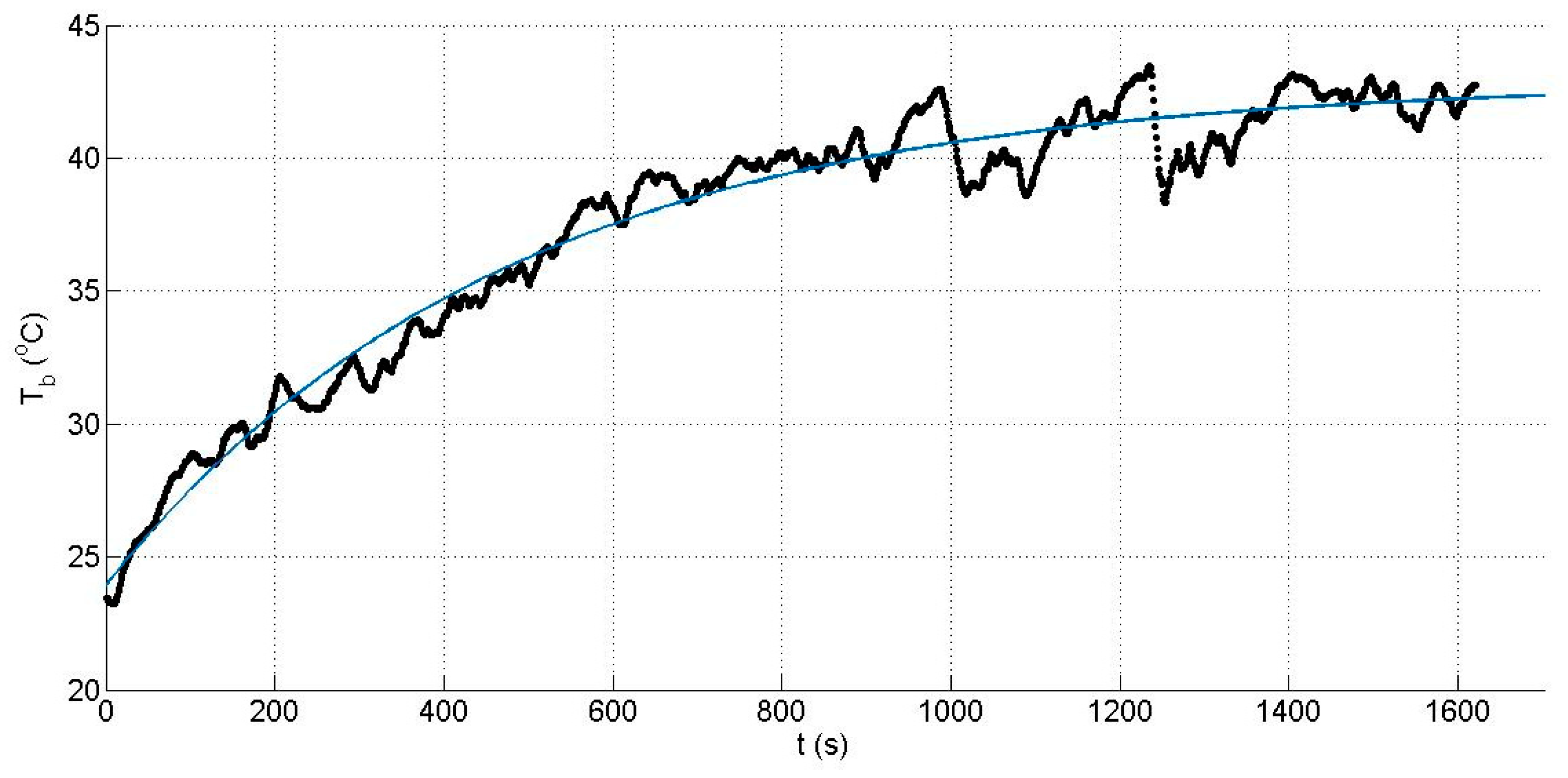
Figure 5 gives measured T_b(t) of a PV module Bioenergy 195W. τ was experimentally determined by the curve fitting analysis and found equal to τ = 316.7 s. For the theoretical prediction of τ, the total heat losses coefficient at field conditions with low v_w was given above equal to 24 W/m² K. According to the values from Table 1, the (mc)_ef normalized to surface A_c for this module, with 3.2 mm glass and PET back sheet of 0.4mm, is estimated in the range of 6760–7720 depending on the c_p of the glass cover. Hence, τ = [6760–7720]:24 = 281.7–321.6 s. In fact, the experimental τ lies inside the domain of the theoretically predicted τ values.

Figure 6 shows the T_b(t) profile of an SM55 module inclined over a window as shadow hanger and power generator, too. The expression F(x) = A(1 − exp(−Bx)) + C was fitted on the data, (upper curve) with R² = 0.959, and gave τ = 306.2 s while the predicted value was determined by setting (mc)_ef 6760 J/m² K (considered for the lower size SM55) and 23–24 W/m² K for the heat losses coefficient. Thus, τ lies in the range 281.7–293.9 s with a deviation of its average from the experimental <6%. However, the wind speed increases at around 1100 s and steady state temperature reached earlier, see lower curve in Figure 6, where the final time constant due to the wind increase shortened τ to 235.7 s, according to the curve analysis. Using (39) [4], a theoretical estimate of τ, is obtained.

U = h_c,f + h_c,b = 11.34 + 7.73v

(39)

which for average wind speed during the experiments v = 1 m/s, as the PV module, operating as a shadow hanger, was in wind protected zone, U = 19.07 W/m² K. Adding 10 W/m² K for h_r,f + h_r,b then, U_pv = 29.07 W/m² K and hence, τ = 6760/29.07 = 232.5 s which is a very good prediction. That shows the strong effect of v_w on PV performance.

3.4. Predicted Steady State T_b(t) Values and Comparison with Measured Data and Results from other Models: Validation of the Proposed Model

The steady state T_b and the f values of pc-Si PV modules operating in field conditions in FIX and ST mounting were experimentally determined and theoretically predicted. The experiments for both FIX and ST PV systems were carried out in months of different environmental conditions, January and July. T_b and f were predicted by:

• the simulation model elaborated and proposed in this article, Equation (10), and
• formulae provided from the other models [1,2,3,4,5,7].

Those f and T_pv values were compared with the experimentally determined ones, shown in

Table 3. Comparison of predicted by this model (T_c − T_a) for morning–noon–afternoon hours in a mid-day of July with the measured values from the FIX and ST and those calculated using models [1,2,3,4,5].

Hour	Model [1]		Model [2]		Model [4]		Model [3]		This Model		Model [5]		Measured *
	F	ST	F	ST	F	ST	F	ST	F	ST	F	ST	F	ST
10	12.9	24	11.4	21.3	10.15	18.8	11.25	21.0	13.6	25.3	12.5	24.1	14.0	23.0
12	20.5	27.3	19.9	26.5	16.25	26.9	20.0	26.6	23.3	27.1	20.4	27.2	23.5	27.3
14	23.2	28.2	22.2	27.1	19	22.2	22.3	27.2	24.1	28.5	22.9	28.0	24.0	29.0
16	16.7	24	13	18.7	12.75	18.55	12.52	18.05	16.5	24	15.4	23.8	17	23

* The fixed inclination (FIX) and ST systems were installed at free environment.

.

In addition,

Table 4. The predicted by this model f values compared with those calculated using models [1,2,3,4,5,7] and the experimentally determined ones, for various hours of a mid-day of January and July under various environmental conditions, I_T and v_w. Both cases of FIX and ST PV systems were considered.

Hour/Type	IT	Tc − Ta	vw	fexp *	fmodel	Model [2]	Model [7]	Model [1]	Model [5]	Model [4]	Model [3]
14 h/7/FIX	840	24.5	2.0	0.0291	0.0303	0.0255	0.0305	0.0245	0.0285	0.0276	0.0278
11 h/7/FIX	623	17	3.8	0.0272	0.0267	0.0195	0.0248	0.0215	0.0227	0.0203	0.0202
16 h/7/ST	970	23	4.2	0.0237	0.0235	0.0184	0.0240	0.0208	0.0237	0.0196	0.0185
16 h/7/FIX	680	16	4.2	0.0235	0.0236	0.0184	0.0240	0.0208	0.0227	0.0220	0.0185
12 h/1/ST	1050	35	1.0	0.0335	0.0340	0.0309	0.0307	0.0264	0.0305	0.0366	0.0300
14 h/1/ST	1020	30.5	2.5	0.0299	0.0286	0.0235	0.0273	0.0236	0.0284	0.0266	0.0264
14 h/1/FIX	800	26.5	2.5	0.0330	0.0340	0.0235	0.0273	0.0236	0.0286	0.0250	0.0264
13 h/1/ST	1080	34.5	1.5	0.0318	0.0337	0.0280	0.0295	0.0254	0.0290	0.0332	0.0322
13 h/1/FIX	860	30.5	1.5	0.0355	0.0330	0.0280	0.0295	0.0254	0.0316	0.0330	0.0322
8 h/7/ST	625	19	1.2	0.0304	0.0318	0.0297	0.0302	0.0260	0.0295	0.0360	0.0343

* f_exp is the f value determined from (T_b − T_a)/I_T measured during the day by a monitoring system.

gives the f values predicted by this model, (10), and also by the known models [1,2,3,4,5,7] during the hours in a mid-day of July and January. In the application presented T_a, v_w and I_T change during the day and the two PV generators sun-tracker and fixed inclination system having identical modules were used. Hence, the tests included two different PV mountings and varying environmental conditions.

It is clear from Table 3 that the proposed model has an overall higher prediction performance over the other models. For this, a statistical analysis on both Tables data provides the consistency and the prediction quality of the models, as shown in Figure 7.

From the results deployed in Table 3 and Table 4 it is clear that the proposed model predicts f and T_pv for FIX and ST configurations systematically very close to the experimentally determined values with deviation less than 4%. The predicted values from models [1,2,3,4,5,7] experience a larger dispersion disclosed by the determination coefficient, R², while their deviations may in general reach up to 15%. In general, the models which do not provide correction due to the effect of I_T, T_a on η_pv exhibit higher deviation compared to this model. Figure 7a–g show the predicted by this model and the models [1,2,3,4,5,7] f values versus the experimental ones. The model proposed exhibits the least dispersion of data and is nearer to the best theoretical line.

4. Discussion

The measured T_b(t) values either for the bare PV cell or the PV modules were best fitted on the function a(1 − exp(t/τ_Tc)), with a coefficient of determination always >0.998, which provided for the τ_Tc. T_b(t) and τ were also predicted theoretically from Equations (29)–(34) accounting for the environmental conditions. The predicted T_b values for a cell deviated by <3% from the measured ones. Both depend on I_T, v_w and the PV geometrical and physico-chemical characteristics, as in Table 1. The dependence on I_T creeps in through the heat transfer coefficients as U_g−a and U_b−a increase with the T_b, which in turn increases with I_T. A formula proposed to predict τ_Tc directly based on Equations (37) and (39) gave very good results, which deviated by <5% from the experimental value. Using more accurate expressions for the U_f and U_b as proposed by the authors in [23], would result in much smaller deviations between the predicted and experimental values but would raise the algorithmic complexity of the model which requires the use of many theoretical expressions to accurately simulate T_pv as analyzed in [23,24], rather than the mixed type compact model proposed here which was the aim of the current work. For the bare c-Si τ_Tc was found equal to 35.8 s–37.1 s for I_T = 10³ W/m², while for c-Si and pc-Si PV modules the τ_Tc value was around 4.5–5.5 min. For v_w higher than 1–2 m/s, τ decreased to 2–2.5 min. This is explained through Equations (32) and (34) where the effect of environmental conditions is expressed through the total effect of U_b−a and U_g−a which inversely affects τ. Note that U_c−b and U_c−g are much larger than U_b−a and U_g−a respectively and therefore the ratio (1 + (U_b−a/U_c−b))/(1 + (U_g−a/U_c−g)) tends to 1. Therefore, the effect of the characteristics of the layers of the module on the time constant is expressed mainly through (mc)_ef in Equations (32) and (34), which proportionally affects τ. For example, the effect of the EVA encapsulant alone is significant as may be estimated using Equation (30) for the modules used in the study the EVA has 15% contribution in the module (mc)_ef value, leading to a larger time constant (by 15%) and more pronounced transient phenomena.

The predicted T_c(t) was used to predict V_oc(t). The result was in excellent agreement with the experimental values for I_T = 10³ W/m². The time constants, τ_Voc, of the theoretically developed V_oc(t) profiles by using (1) lie very close to the experimentally determined ones. The transient prediction model is easily handled even for I_T and v_w changing during monitoring. The introduction of the I_T(t) and v_w(t) values into the algorithm, Equations (31)–(33), is done using their average values in each time unit. The recorded steady state T_b values during the hours of the mid-day of 2 climatically opposite months, July and January, were compared with the predicted values. An excellent agreement was confirmed and the diagram of the predicted by this model f values versus experimental ones was of higher quality compared to the other models. It is important to underline that the constants a, b, c in Equations (9) and (10) were derived by regression analysis of data taken from the operation of 7 years old pc-Si modules. Therefore, an ageing correction, of +7 years × 0.85%/year = +6% must be added in the predicted f values obtained from the other models [1,2,3,7], provided that those models were developed using brand new PV modules. Thus, a good improvement will be achieved in their prediction performance. Finally, it is emphasized that the experimentally determined f and T_b values used in the validation test were excluded from the data used in the regression analysis to build the f(v_w) quadratic formula.

The model developed applies to free standing PV modules or cells in any environmental conditions. It is based on c-Si PV modules but could be easily adapted to flat plate PV modules of other types as long as the properties of Table 1 are enriched for the layers and composition of these types. The model would need to be adapted for PV modules inclined before windows and BIPV as it concerns the view factor and the convection coefficients. The steady state model takes into account wind velocity but not wind direction, while module inclination is not considered. These can be integrated into the model through U_f and U_b as in [23] and will be presented in future work.

5. Conclusions

A new model to predict the steady state PV cell or module temperature, T_pv or T_b with a version to predict the transient temperature profiles was elaborated, presented, and validated. The model is based on a quadratic v_w function multiplied with a correction function accounting for the change in η_pv due to the deviation of the environmental conditions from their average values taken as reference. An excellent agreement under any environmental conditions was confirmed between predicted and recorded PV module T_b values, deviation <3%, in comparison with other 6 known models. The model performed better than any other one. Accurate PV temperature prediction is especially important considering its significant effect on PV power output, with a typical value for the temperature coefficient of P_m of −0.5%/°C. Considering that a range of 5–25% reduction in power output is normally expected from the nominal value for 1000 W/m² incident irradiance due to PV temperature alone, accurate prediction of PV temperature can assist in adequate control measures, monitoring and diagnostic procedures to be taken in practical situations of PV installations.

Finally, a mathematical algorithmic expression was developed to predict the transient T_b(t), T_g(t), T_c(t). The time constant of the T_b(t) profiles for the PV modules theoretically derived and experimentally determined deviated by less than 5%. The accuracy can be further increased with a more analytical determination of U_f and U_b as in [23]. The transient model provided also a simple expression for the steady state T_b whose deviation from the theoretical and experimental values was less than 5.8%. The transient T_b(t) profile produced by the model followed closely the measured T_b data, as was shown in many cases examined in a bare c-Si cell and also in 3 c-Si and pc-Si PV modules. The compact model developed is applicable to any geographical site and environmental conditions.

References

- King, D.L.; Boyson, W.E.; Kratochvill, J.A. Photovoltaic Array Performance Model; SAND2004-3535; Sandia National Laboratories: Albuquerque, NM, USA; Livermore, CA, USA, 2004.
- Faiman, D. Assessing the outdoor operating temperature of photovoltaic modules. Prog. Photovolt. Res. Appl. 2008, 16, 307–315. [Google Scholar] [CrossRef]
- Skoplaki, E.; Palyvos, J.A. On the temperature dependence of photovoltaic module electrical performance: A review of efficiency/power correlations. Sol. Energy 2009, 83, 614–624. [Google Scholar] [CrossRef]
- Mattei, M.; Notton, G.; Cristofari, C.; Muselli, M.; Poggi, P. Calculation of the polycrystalline PV module temperature using a simple method of energy balance. Renew. Energy 2006, 31, 553–567. [Google Scholar] [CrossRef]
- Mani, T.G.; Ji, L.; Tang, Y.; Petacci, L.; Osterwald, C. Photovoltaic Module Thermal/Wind Performance: Long Term Monitoring and Model Development for Energy Rating. In Proceedings of the NCPV and Solar Program Review Meeting, Denver, CO, USA, 24–26 March 2003. [Google Scholar]
- Fuentes, M.K. A Simplified Thermal Model for Flat-Plate Photovoltaic Modules; SAND85-0330 UC-63; Sandia National Laboratories: Albuquerque, NM, USA; Livermore, CA, USA, 1987.
- King, D.L. Photovoltaic module and array performance characterization methods for all system operating conditions. In Proceedings of the NREL/SNL Photovoltaics Program Review Meeting, Lakewood, CO, USA, 18–22 November 1996; AIP Press: New York, NY, USA, 1997. [Google Scholar]
- Mora Segado, M.; Carretero, J.; Sidrach-de-Cardona, M. Models to predict the operating temperature of different photovoltaic modules in outdoor conditions. Prog. Photovolt. Res. Appl. 2015, 23, 1267–1282. [Google Scholar] [CrossRef]
- Hammami, M.; Torretti, S.; Grimaccia, F.; Grandi, G. Thermal and Performance analysis of a Photovolatic Module with an Integrated Energy Storage System. Appl. Sci. 2017, 7, 1107. [Google Scholar] [CrossRef]
- Ciulla, G.; Lo Brano, V.; Moreci, E. Forecasting the cell temperature of PV modules with an adaptive system. Int. J. Photoenergy 2013, 2013, 192854. [Google Scholar] [CrossRef]
- Kaplanis, S. Determination of the electrical characteristics and thermal behaviour of a c-Si cell under transient conditions for various concentration ratios. Int. J. Sustain. Energy 2016, 35, 887–992. [Google Scholar] [CrossRef]
- Tina, G.M.; Marletta, G.; Sardella, S. Multy-layer thermal models of PV modules for monitoring applications. In Proceedings of the 38th IEEE Photovoltaic Specialists Conference, Austin, TX, USA, 3–8 June 2012. [Google Scholar] [CrossRef]
- Jones, A.D.; Underwood, C.P. A Thermal Model for Photovoltaic Systems. Sol. Energy 2001, 70, 349–359. [Google Scholar] [CrossRef]
- Shahzada, P.A.; Ahzi, S.; Barth, N.; Abdallah, A. Using energy balance method to study the thermal behavior of PV panels under time varying field conditions. Energy Convers. Manag. 2018, 175, 246–262. [Google Scholar]
- Kayhan, O. A thermal model to investigate the power of solar array for stratospheric balloons in real conditions. Appl. Therm. Eng. 2018, 139, 13–120. [Google Scholar] [CrossRef]
- Brinkworth, B.J.; Marshall, R.H.; Ibarahim, Z. A validated model of naturally ventilated PV cladding. Sol. Energy 2000, 69, 67–81. [Google Scholar] [CrossRef]
- Armstrong, S.; Hurley, W.G. A thermal model for photovoltaic panels under varying atmospheric conditions. Appl. Therm. Eng. 2010, 30, 1488–1495. [Google Scholar] [CrossRef]
- Trinuruk, P.; Sorapipatana, C.; Chenvidhya, D. Estimating operating cell temperature in BIPV modules in Thailand. Renew. Energy 2009, 34, 2515–2523. [Google Scholar] [CrossRef]
- AssoaYa, B.; Zamini, S.; Sprenger, W.; Misara, S.; Pellegrino, M.; Erleaga, A.A. Numerical Analysis of the Impact of Environmental Conditions on BIPV: An Overview of the BIPV Modelling in SOPHIA Project. In Proceedings of the 27th European Photovoltaic Solar Energy Conference and Exhibition, Frankfurt, Germany, 24–28 September 2012; pp. 4143–4149. [Google Scholar]
- Jakhrany, A.Q.; Othman, A.K.; Rigit, A.R.H.; Samo, S.R. Comparison of Solar Photovoltaic Temperature Models. World Appl. Sci. J. 2011, 14, 1–8. [Google Scholar]
- Kaplanis, S.; Kaplani, E. A PV temperature prediction model for BIPV configurations, comparison with other models and experimental results. In Proceedings of the 9th International Workshop on Teaching in Photovoltaics (IWTPV 2018), Prague, Czech Republic, 15–16 March 2018; Ceske Centrum IET. pp. 20–26. [Google Scholar]
- Kamuyu, W.C.L.; Lim, J.R.; Won, C.S.; Ahn, H.K. Prediction model of Photovoltaic Module Temperature for Power Performance of Floating PVs. Energies 2018, 11, 447. [Google Scholar] [CrossRef]
- Kaplani, E.; Kaplanis, S. Thermal modelling and experimental assessment of the dependence of PV module temperature on wind velocity and direction, module orientation and inclination. Sol. Energy 2014, 107, 443–460. [Google Scholar] [CrossRef] [Green Version]
- Kaplani, E.; Kaplanis, S. PV module temperature prediction at any environmental conditions and mounting configurations. In Proceedings of the World Renewable Energy Congress (WREC’18), London, UK, 30 July–3 August 2018. [Google Scholar]
- Akhasassi, M.; El Fathi, A.; Erraissi, N.; Aarich, N.; Bennouna, A.; Raoufi, M.; Outzourhit, A. Experimental investigation and modeling of the thermal behaviour of a solar PV module. Sol. Energy Mater. Sol. Cells 2018, 180, 271–279. [Google Scholar] [CrossRef]
- KouadriBoudjelthia, E.A.; Abbas, M.L.; Semaoui, S.; Kerkouche, K.; Zeraïa, H.; Yaïche, R. Role of the wind speed in the evolution of the temperature of the PV module: Comparison of prediction models. Rev. Energies Renouvelables 2016, 19, 119–126. [Google Scholar]
- Schwingshackl, C.; Petitta, M.; Wagner, J.E.; Belluardo, G.; Moser, D.; Castelli, M.; Zebisch, M.; Tetzlaff, A. Wind effect on PV module temperature: Analysis of different techniques for an accurate estimation. Energy Procedia 2013, 40, 77–86. [Google Scholar] [CrossRef]
- Mittelman, G.; Alshare, A.; Davidson, J.H. A model and heat transfer correlation for rooftop integrated photovoltaics with a passive air cooling channel. Sol. Energy 2009, 83, 1150–1160. [Google Scholar] [CrossRef]
- Saadon, S.; Gaillard, L.; Giroux-Julien, S.; Menezo, C. Simulation study of a naturally-ventilated building integrated photovoltaic/thermal, BIPV/T, envelope. Renew. Energy 2016, 87, 517–531. [Google Scholar] [CrossRef]
- Ciulla, G.; Lo Brano, V.; Franzitta, V.; Trapanese, M. Assessment of the operating temperature of crystalline PV modules based on real use conditions. Int. J. Photoenergy 2014, 2014, 718315. [Google Scholar] [CrossRef]
- Rubin, L.; Nebusov, V.; Leutz, R.; Schneider, A.; Osipov, A.; Tarasenko, V. DAY4TM PV Receivers and Heat Sinks for Sun Concentration Applications. In Proceedings of the 4th International Conference on Solar Concentrators for the Generation of Electricity or Hydrogen, El Escorial, Spain, 12–16 March 2007. [Google Scholar]
- Peng, C.; Yang, J. The effect of Photovoltaic Panels on the Rooftop Temperature in the EnergyPlus Simulation Environment. Int. J. Photoenergy 2016, 2016, 9020567. [Google Scholar] [CrossRef]
- Misara, S. Thermal Impacts on Building Integrated Photovoltaics (BIPV). Ph.D. Thesis, Universitat Kassel, Kassel, Germany, 2014. [Google Scholar]
- Lienhard, J.H., IV; Lienhard, J.H., V. A Heat Transfer Textbook, 3rd ed.; Phlogiston Press: Cambridge, MA, USA, 2000. [Google Scholar]
- Dupont, Tedlar PVF Films for Industrial Applications. Available online: www.tedlar.com (accessed on 20 October 2018).
- Webb, J.E.; Wilcox, D.I.; Wasson, K.L.; Gulati, S.T. Specialty thin glass for PV modules: Mechanical Reliability Considerations. In Proceedings of the 24th European Photovoltaic Solar Energy Conference and Exhibition, Hamburg, Germany, 21–25 September 2009. [Google Scholar]
- Ross, R.G. Interface design considerations for terrestrial solar cell modules. In Proceedings of the 12th IEEE Photovoltaic Specialist’s Conference, Baton Rouge, LA, USA, 15–18 November 1976; pp. 801–806. [Google Scholar]
- D‘Orazio, M.; Di Perna, C.; Di Giuseppe, E. Experimental operating cell temperature assessment of BIPV with different installation configurations on roofs under the Mediterranean climate. Renew. Energy 2014, 68, 378–386. [Google Scholar] [CrossRef]
- Muller, M.T.; Rodriguez, J.; Marion, B. Performance comparison of a BIPV roofing tile system in two mounting configurations. In Proceedings of the 2009 34th IEEE Photovoltaic Specialists Conference, Philadelphia, PA, USA, 7–12 June 2009. [Google Scholar]
- Pantic, S.; Candanedo, L.; Athienitis, A.K. Modeling of energy performance of a house with three configurations of building-integrated photovoltaic/thermal systems. Energy Build. 2010, 42, 1779–1789. [Google Scholar] [CrossRef]
- Kaplanis, S.; Kaplani, E. On the relationship factor between the PV module temperature and the solar radiation on it for various BIPV configurations. AIP Conf. Proc. 2014, 1618, 341–347. [Google Scholar] [CrossRef] [Green Version]
Figure 1.
A schematic section of a photovoltaic (PV) module with its characteristic layers. EVA: Ethylene-vinyl Acetate, ARC: Anti-reflective Coating.
Figure 2.
f versus t as determined for the mid-day of March with parameters vw and IT. The strong impact of vw on f is obvious. (a) Corresponds to the FIX PV system and (b) to the sun tracking (ST) one.
Figure 3.
Predicted Tb,pred(t) and measured Tb,meas(t) profiles of a c-Si bare cell in controlled laboratory conditions.
Figure 4.
Predicted Voc,pred(t) and measured Voc,meas(t) profiles for a bare c-Si cell in controlled laboratory conditions.
Figure 5.
Tb(t) profile for a c-Si Bioenergy 195W PV module in field conditions.
Figure 6.
Tb(t) profile SM55 module placed inclined over a window in a Building Adapted Photovoltaics (BAPV) configuration.
Figure 7.
Results from a regression analysis of predicted f values versus the experimentally determined f values where f is predicted by (a) the proposed model, (b) model [2], (c) model [1], (d) model [7], (e) model [5], (f) model [4], and (g) model [3].