Thermal Characteristics Investigation of the Internal Combustion Engine Cooling-Combustion System Using Thermal Boundary Dynamic Coupling Method and Experimental Verification

Abstract

The engine cooling system must be able to match up with the stable operating conditions so as to guarantee the engine performance. On the working cycle level, however, the dynamic thermo-state of engines has not been considered in the cooling strategy. Besides, the frequent over-cooling boiling inside the gallery changes the cooling capacity constantly. It is necessary to study the coupling effect caused by the interaction of cooling flow and in-cylinder combustion so as to provide details of the dynamic control of cooling systems. To this end, this study develops a coupled modeling scheme of the cooling process considering the interaction of combustion and coolant flow. The global reaction mechanism is used for the combustion process and the multiphase flow method is employed to simulate the coolant flow considering the wall boiling and the interphase forces. The two sub-models exchange information of in-cylinder temperature, heat transfer coefficient, and wall temperature to achieve the coupled computation. The proposed modeling process is verified through the measured diesel engine power, in-cylinder pressure, and fire surface temperature of cylinder head. Then the effects of different cooling conditions on the cyclic engine performances are analyzed and discussed.

1. Introduction

Concerning the energy and environment performances of diesel engines, efficiency is an increasingly important issue since only 30% to 40% of the fuel energy is transformed into mechanical work. As a main part of energy loss, the cooling process affects the combustion by means of the cylinder wall temperature. Generally the cooling strategy is correlated to the engine speed, which would result in overcooling effects in operation [1].

To simulate the cooling procedure, Jung et al. [2] combined multiple models of thermal mass, coolant, lubricant, heat transfer, friction and exhaust. A variable-speed water pump with proper coolant flow control was adopted to increase the fuel economy by about 2.5%. Based on thermal management modeling, Kang [3] designed a double loop coolant circuit for the cylinder head and engine block, which indicates 30% coolant flow rate of the basic system can satisfy the thermal requirement of the target engine. Wang [4] presented a nonlinear adaptive control strategy for a radiator fan matrix for transient engine temperature tracking and the power consumption was reduced greatly. Zhou [5] developed a 1D model to simulate the thermal management system by combining the coolant circuit and the oil circuit together. The proposed strategy makes the engine operate under an appropriate temperature and the total power consumption can be significantly reduced. Reference [6] shows that the fuel consumption can be reduced by 1–3% by using electrified cooling systems and advanced thermal topologies. For emissions, it has been presented that increasing the in-cylinder temperature by increasing the coolant temperature can reduce Total Hydrocarbons (THC) and carbon monoxide (CO) but increase nitrogen oxides (NO_x) [7].

A certain portion of gas bubbles in the liquid can produce a turbulent regime to increase heat transfer, so the presence of bubbles in the coolant could be an effective tool to improve the engine cooling efficiency. On this basis, Reference [8] set up a controlled air injection into the engine coolant inlet to generate bubbles, which can reduce the warm-up time by injecting a large amount of air and enhance the heat transfer by making a few bubbles under normal working condition. The nuclear flow boiling in the gallery, which can be regarded as a gas-liquid two phase flow, has a similar mechanism as the air injection that can improve the heat transfer capability in addition to the phase change heat transfer. Without extra equipment, the nuclear boiling heat transfer flow generates gas bubbles automatically under certain superheated temperature conditions. The occurrence of nuclear flow boiling depends on the operational conditions, including pressure, temperature and flow rate. Castiglione et al. [9,10,11] conducted a series of studies on the nuclear boiling operation conditions for engine cooling systems. The relationship between the flow rate and the nuclear boiling onset was studied under a constant engine speed [10]. According to the calculated nuclear boiling heat transfer, a control strategy for the cooling system under nuclear boiling conditions was presented [11], which is proved effective in decreasing the warm-up time as well as in reducing the coolant flow rate under fully warmed conditions. It can be found the nuclear boiling is beneficial to the engine cooling, which can provide faster warm-up and lower friction with smaller coolant mass, smaller radiator and lower pump power.

Most studies for engine cooling control are conducted in steady state, which means the control strategies are developed separately for different operation conditions. Although the engine can be considered working stably in a certain load case, the thermal state and the cooling process within a working cycle are still crankshaft angle-dependent. It is necessary to extract the correlation between the cooling system and the in-cylinder work in cycle level in order to provide detailed information for engine cooling control. Two issues should be highlighted: (1) whether the microscopic transient changes in the cooling conditions are effective to achieve power changes; (2) how to achieve a change in cooling conditions. This article focuses on the first issue. If the dynamic response of cooling and combustion coupling is achieved by simulation, the most accurate method is three-dimensional (3-D) coolant simulation and combustion simulation with thermal coupling through the wall of the combustion chamber. However, the computational cost is high and multi-field coupling simulation is very difficult. Moreover, the one-dimensional (1-D) combustion model also has good accuracy in engine power, so the 1-D combustion is selected to solve the change in the energy consumption in the cylinder. To this end, a coupled modeling process is proposed combined of 3-D coolant nuclear flow boiling and 1-D combustion. The two major simulation parts iteratively exchange wall temperature, in-cylinder temperature and heat transfer coefficient information. Using the coolant rated flow and the inlet temperature as design variables, the effects of cooling parameters on engine performances are analyzed and discussed. This article only researches the change law of engine thermal characteristics under changing cooling conditions by a simulation method and proposes a control concept for intelligent engine cooling control. It does not involve the actual engineering means of how to achieve any cooling conditions changes.

2. Modelling Process

2.1. In-Cylinder Model

This article mainly studies the energy change of the engine due to the cooling conditions variation, which does not include a detailed study on the combustion of the chemical reaction and combustion turbulent flow in the engine, so the simplified 1-D combustion is used to describe the in-cylinder energy change.

2.1.1. Energy Conservation

The in-cylinder thermodynamic state calculation is based on the first law of thermodynamics:

$$\frac{d\left(m_{c}u\right)}{dt}=-p_c\cdot \frac{dV}{dt}+\frac{d{Q}_F}{dt}-{\displaystyle \sum \frac{d{Q}_w}{dt}}+Q_{in}+Q_{out}+Q_{oth}$$

(1)

where m_c is the in-cylinder mass and u is the internal energy of unit mass, $p_c$ is the in-cylinder gas pressure, $V$ is the actual cylinder volume, Q_F is the fuel heat input, Q_w is the wall heat loss, $Q_{in}$ is the heat of inflow, $Q_{out}$ is the heat of outflow, and $Q_{oth}$ is the residual heat loss.

As reported in Taymaz et al. [12] the heat transfer to the coolant reaches 30%~50% of fuel energy at 20%~80% load, and the remainder heat loss is only 1% of the fuel energy. Tauzia [13] stated that, in the total energy, the cooling loss accounts for about 35%, the exhaust loss is about 25% and the output work is about 35%, so it is reasonable to neglect the rest of the heat loss in the following study. The total energy generated by combustion is divided into three parts: the output work, the energy change, and the wall heat loss. Some assumptions are defined. The fuel added to the cylinder charge is immediately combusted, and the combustion products mix instantaneously with the rest of the cylinder charge and form a uniform mixture. The gas flow rate is calculated by in-cylinder pressure and volume. As assumed that the in-cylinder gas is ideal, the pressures of compression stroke and power stroke can be obtained as follows:

$$p_c\cdot V=n\cdot R\cdot T$$

(2)

where $n$ is the number of moles of gas, and $R$ is the gas constant. Similarly, the number of moles of air in the intake or exhaust stroke can be obtained using the intake pressure and the in-cylinder pressure.

2.1.2. Combustion

A 1-D combustion model is adopted to simulate the in-cylinder combustion. The combustion chemical reaction is simplified through the global reaction mechanism as follows:

$$\begin{array}{l}{\mathrm{C}}_x{\mathrm{H}}_y+\left(x+\frac{y}{4}\right){\mathrm{O}}_2\stackrel{k_G}{\circledR }x\mathrm{C}{\mathrm{O}}_2+\frac{y}{2}{\mathrm{H}}_2\mathrm{O}\frac{dy}{dx}\\ \frac{d\left[{\mathrm{C}}_x{\mathrm{H}}_y\right]}{dt}=-k_G{\left[{\mathrm{C}}_x{\mathrm{H}}_y\right]}^a{\left[{\mathrm{O}}_2\right]}^b\end{array}$$

(3)

where $k_G$ is the global rate coefficient related to temperature. Using the Arrhenius form, the global rate coefficient is:

$$k_G(T)=Aexp\left(-E_A/RT\right)$$

(4)

The diesel fuel is represented by C₇H₁₆ with rate coefficients A = 5.1 × 10¹¹ mol/(cm³s), E_A = 30 kcal/mol, a = 0.25, b = 1.5, 44,926 kJ/kg of lower Heating Value [14]. Then the fuel heat input $\frac{d{Q}_F}{dt}$ is calculated according to Equations (3) and (4).

2.1.3. Heat Transfer

The heat transfer to the walls of the combustion chamber, i.e., the fire surface of the cylinder head, the piston top surface, and the cylinder liner, is calculated from:

$$Q_{wi}=A_i\cdot a_w\cdot \left(T_c-T_{wi}\right)$$

(5)

where $Q_{\mathrm{wi}i}$ is the wall heat flow, $A_i$ is the surface area, $a_w$ is the heat transfer coefficient, $T_c$ is the in-cylinder gas temperature, and $T_{wi}$ is the wall temperature. The Hohenberg model [15] is adopted in this simulation as follows:

$$a_w=130\times V^{-0.06}\cdot p_c^{0.8}\cdot T_c^{-0.4}\cdot {\left(c_m+1.4\right)}^{0.8}$$

(6)

where V is the actual cylinder volume, $p_c$ is the in-cylinder pressure, and $c_m$ is the mean piston speed. The one-dimensional model [16] is used to predict the heat transfer coefficient in the inlet and exhaust of the engine:

$$Nu=0.032\mathrm{R}{\mathrm{e}}^{0.8}\mathrm{P}{\mathrm{r}}^{0.43}2\times {10}^5\le \mathrm{R}\mathrm{e}\le 5\times {10}^6$$

(7)

2.2. Nuclear Boiling Model

In some regions of the cooling gallery, phase change occurs in the coolant due to superheat wall temperature, which converts the convection heat transfer to a more efficient mode—the nuclear boiling heat transfer. The flow boiling model based on Eulerian multiphase flow method is used.

The continuity equation for phase $q$ is:

$$\frac{\partial }{\partial t}\left({\alpha }_q{\rho }_q\right)+\nabla \left({\alpha }_q{\rho }_q{\overrightarrow{u}}_q\right)={\displaystyle \sum _{p=1}^n\left({\dot{m}}_{pq}-{\dot{m}}_{qp}\right)}+S_q$$

(8)

The momentum equation for phase $q$ is:

$$\frac{\partial }{\partial t}\left({\alpha }_q{\rho }_q{\overrightarrow{u}}_q\right)+\nabla \left({\alpha }_q{\rho }_q{\overrightarrow{u}}_q{\overrightarrow{u}}_q\right)=-{\alpha }_q\nabla p+\nabla {\tau }_q+{\alpha }_q{\rho }_q\overrightarrow{g}+{\displaystyle \sum _{p=1}^n\left({\dot{m}}_{pq}{\overrightarrow{u}}_{pq}-{\dot{m}}_{qp}{\overrightarrow{u}}_{qp}\right)}+{\displaystyle \sum \overrightarrow{F}}$$

(9)

The energy equation for phase $q$ is:

$$\frac{\partial }{\partial t}\left({\alpha }_q{\rho }_q{h}_q\right)+\nabla \left({\alpha }_q{\rho }_q{\overrightarrow{u}}_q{h}_q\right)=-{\alpha }_q\frac{\partial p_q}{\partial t}+{\tau }_q:\nabla {\overrightarrow{u}}_q-\nabla {\overrightarrow{q}}_q+S_{source,q}+{\displaystyle \sum _{p=1}^n\left(Q_{pq}+{\dot{m}}_{pq}{h}_{pq}-{\dot{m}}_{qp}{h}_{qp}\right)}$$

(10)

where $u$ is the velocity, $p$ is the pressure, $\alpha$ is the void fraction, $\rho$ is the density, $m$ is the mass, and $S$ is the source term. The wall boiling model is used for the heat transfer, and the phase interaction force is used for the momentum transfer.

2.2.1. Wall Boiling

The wall boiling heat equations are:

$$q=q_{con}+q_e+q_q$$

(11)

$$q_{con}=h_c\left(T_w-T_l\right)\left(1-A_b\right)$$

(12)

$$q_e=m_b{N}_w{h}_{lg}$$

(13)

$$q_q=\frac{2k_l\sqrt{f}}{\sqrt{\pi {\lambda }_l}}\left(T_w-T_l\right)$$

(14)

where q is the total heat flux, q_con is the convection heat flux, q_e is the gas evaporation latent heat flux, $T_w$ and $T_l$ are the wall temperature and the liquid temperature, $h_c$ is the convection heat transfer coefficient, $h_{lg}$ is the latent heat, $A_b$ is the wall area covered by gas, $\left(1-A_b\right)$ is the wall area covered by liquid, $m_b$ is the mass of the bubble based on the bubble departure diameter, $N_w$ is the nucleation sites density, and $f$ is the bubble departure frequency. The gas covered wall area $A_b$ is a function of the bubble departure diameter $d_d$ and the nucleation sites density:

$$\begin{array}{l}{A}_b=K\frac{N_w\pi d_d^2}{4}\\ K=4.8e^{\left(-\frac{Ja}{80}\right)}\end{array}$$

(15)

where K is the empirical constant and Ja is Jakob number.

The bubble departure diameter [17], the bubble departure frequency [18] and the nucleation sites density [19] can be expressed as:

$$d_d=\mathrm{m}\mathrm{i}\mathrm{n}\left(0.0014,0.0006{\mathrm{e}}^{-\frac{\Delta T_w}{45}}\right)$$

(16)

$$f=\sqrt{\frac{4g\left({\rho }_l-{\rho }_v\right)}{3{\rho }_l{d}_d}}$$

(17)

$$N_w={210}^{1.805}{\left(T_w-T_{sat}\right)}^{1.805}$$

(18)

where T_w is the saturation temperature.

2.2.2. Phase Interaction

The phase interaction force $\overrightarrow{F}$ is

$${\displaystyle \sum \overrightarrow{F}}={\overrightarrow{F}}_{drag}+{\overrightarrow{F}}_{lift}+{\overrightarrow{F}}_{vm}+{\overrightarrow{F}}_{TD}+{\overrightarrow{F}}_{WL}$$

(19)

where ${\overrightarrow{F}}_{drag}$ is the drag force and aroused by interfacial friction force and pressure difference, ${\overrightarrow{F}}_{lift}$ is the lift force due to velocity gradients in the primary-phase flow field, ${\overrightarrow{F}}_{vm}$ is the virtual mass force caused by the secondary phase acceleration relative to the primary phase, ${\overrightarrow{F}}_{WL}$ is the wall lubrication force in the lateral direction tending to push the secondary phase away from the wall, and ${\overrightarrow{F}}_{TD}$ is the turbulent dispersion force which acts as a turbulent diffusion in dispersed flows accounting for the interphase turbulent momentum transfer.

The drag force between the gas phase g and liquid phase l is:

$$F_{drag}=0.75\frac{{\alpha }_g{\rho }_l{C}_D\Delta u^2}{d_b}$$

(20)

where $d_b$ is the bubble diameter, $\Delta u$ is the velocity difference of two phase, $C_D$ is the drag force coefficient [20]

$$\begin{array}{l}{C}_D=24\left(1+0.15\mathrm{R}{\mathrm{e}}^{0.687}\right)/\mathrm{R}\mathrm{e}\\ C_D=0.44\end{array}\begin{array}{l}\hspace{1em}\mathrm{R}\mathrm{e}\ge 1000\\ \hspace{1em}\mathrm{R}\mathrm{e}>1000\end{array}$$

(21)

The lift force acting on a secondary phase p in a primary phase q is:

$${\overrightarrow{F}}_{lift,q}=-C_l{\alpha }_g\left({\overrightarrow{u}}_q-{\overrightarrow{u}}_p\right)\times \left(\tilde{N}\times {\overrightarrow{u}}_q\right)$$

(22)

where $C_l$ is the lift force coefficient [21]:

$$\begin{array}{c}{C}_l=\{\begin{array}{l}0.0767\\ -\left(-0.12-0.2e^{-\frac{\phi }{3.6}\times {10}^{-5}}\right)e^{\frac{\phi }{3}\times {10}^{-7}{}^{}}\\ -0.6353\end{array}\begin{array}{l}\phi \le 6000\\ 6000<\phi <5\times {10}^7\\ \phi \ge 5\times {10}^7\end{array},\\ \phi =\frac{{\rho }_q^2\left|{\overrightarrow{u}}_q-{\overrightarrow{u}}_p\right|\times \left|\tilde{N}\times {\overrightarrow{u}}_q\right|d_p^3}{{\mu }_q^2}\end{array}$$

(23)

The virtual mass force acting on a secondary phase p in a primary phase q is:

$${\overrightarrow{F}}_{vm,q}={\alpha }_q{\rho }_p{C}_{vm}\left(\frac{d{\overrightarrow{u}}_q}{dt}-\frac{d{\overrightarrow{u}}_p}{dt}\right)$$

(24)

where $C_{vm}$ is the virtual mass force coefficient with a typically value of 0.5.

The wall lubrication force acting on a secondary phase p in a primary phase q is:

$${\overrightarrow{F}}_{WL}=C_{WL}{\rho }_q{\alpha }_q{\left|{\overrightarrow{u}}_q-{\overrightarrow{u}}_p\right|}^2{\overrightarrow{n}}_w$$

(25)

where $C_{WL}$ is the wall lubrication force coefficient [22].

$$C_{WL}=max\left(0,\frac{-0.001}{d_b}+\frac{0.05}{y_w}\right)$$

(26)

where $d_b$ is the bubble/particle diameter and $y_w$ is the distance to the nearest wall.

The turbulent dispersion force between the gas phase g and liquid phase l is [23]:

$$F_{TD}=\frac{3{\alpha }_g{\rho }_l{C}_D\Delta u^2}{4d_b}\frac{{\mu }_{tl}}{{\delta }_k{\rho }_l}\left(\frac{\tilde{N}{\alpha }_g}{{\alpha }_g}-\frac{\tilde{N}{\alpha }_l}{{\alpha }_l}\right)$$

(27)

2.3. Modelling Scheme

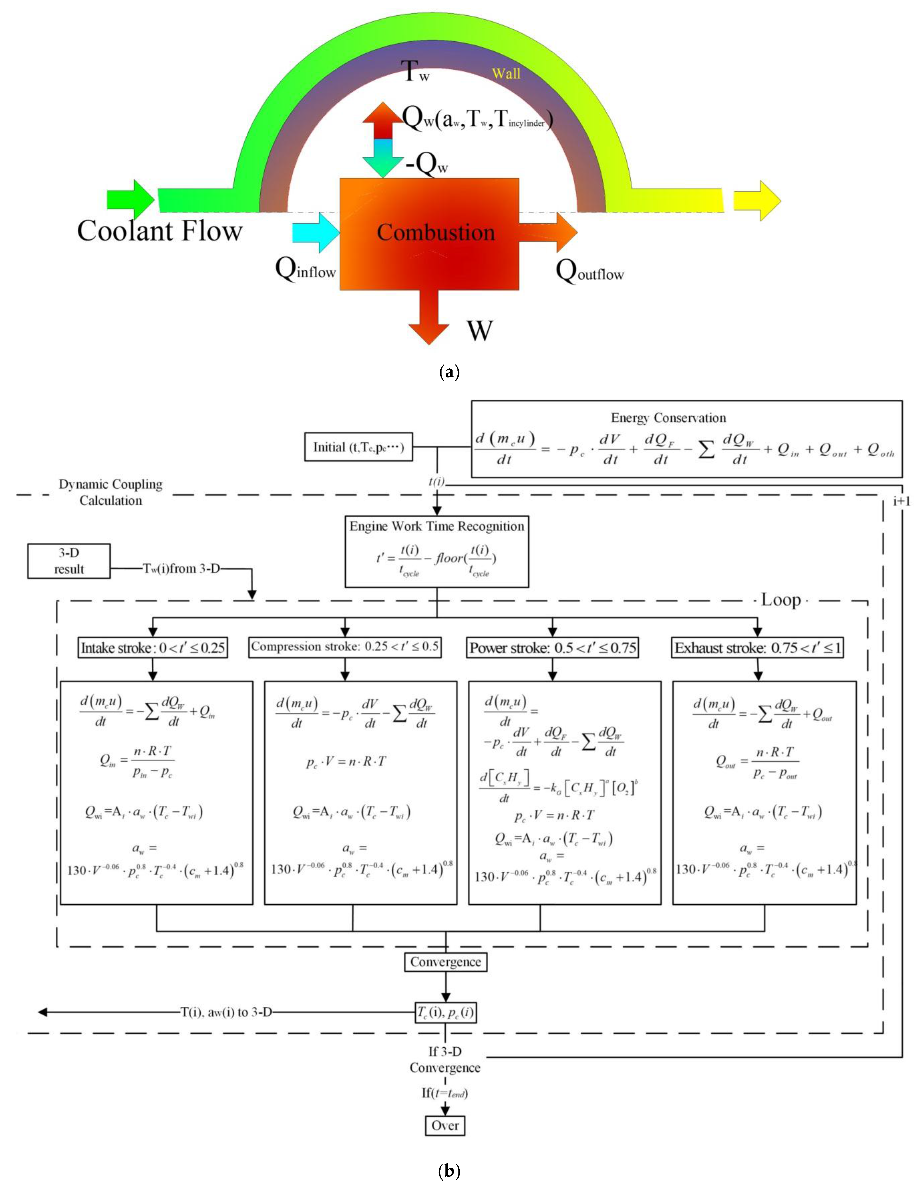
The heat loss from the piston is approximately calculated by the average temperature of the gas and combustion chamber and heat transfer coefficient. The dynamic relationship between cooling and combustion is shown in Figure 1a. The piston work and the heat of inflow and outflow are defined in Equation (1), and the wall heat flow is described in Equation (5). The two independent variables, the in-cylinder pressure and temperature, are used as the criteria for the convergence of the 1-D combustion equation. The wall temperature can be determined by the dynamic reaction of cooling and combustion. 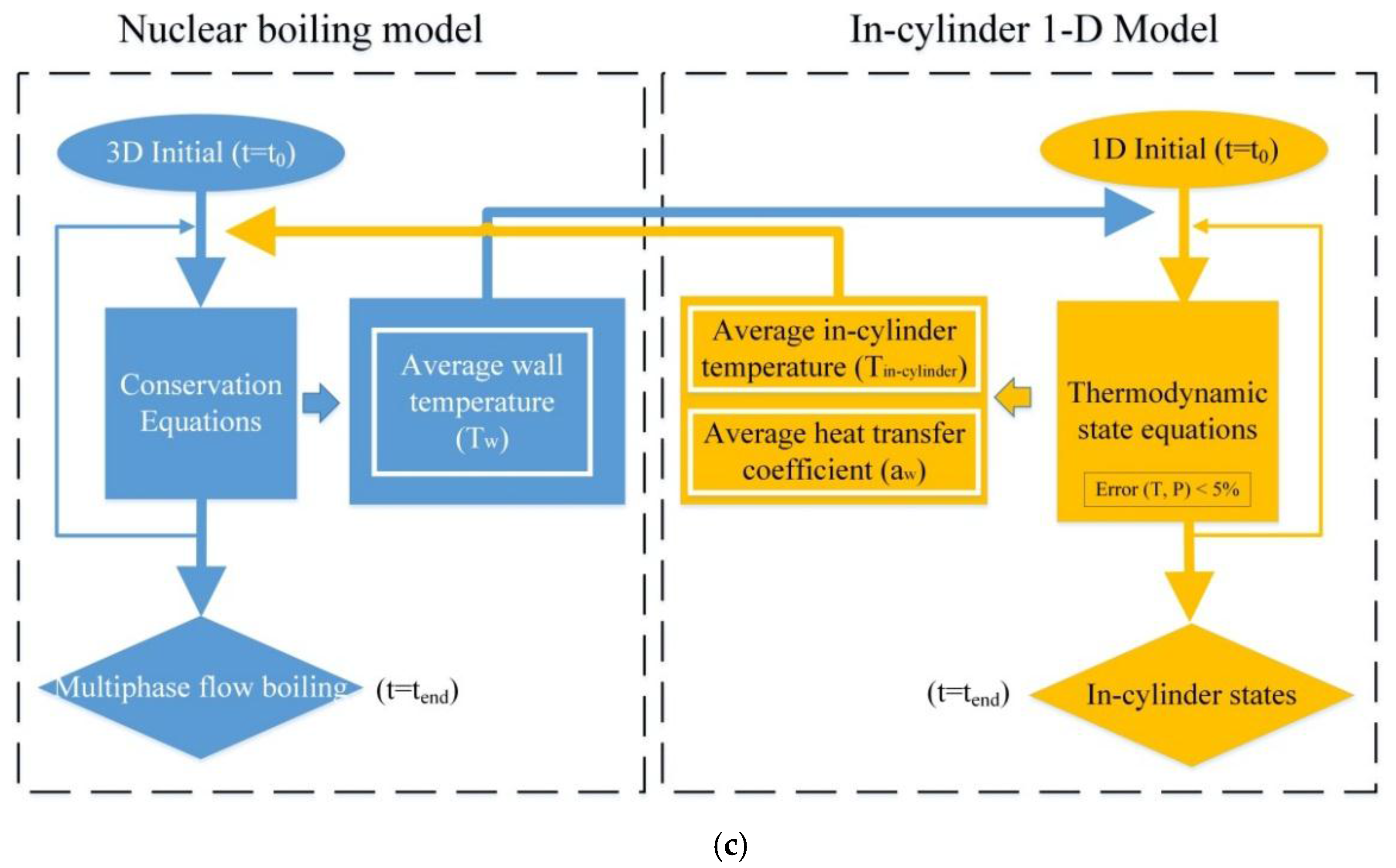All of these calculations are shown in Figure 1b. The coupled simulation of cooling and combustion is carried out according to the scheme shown in Figure 1c. In the 3-D simulation of coolant flow, the wall temperature can be obtained through the third type thermal boundary condition, where the heat transfer coefficient and the in-cylinder temperature are provided by the 1-D simulation. Iterations are executed on both parts with the dynamic information exchange in every time step: one is the loop for combustion pressure and temperature, the other is the multiphase turbulent flow solution. The 1-D combustion model is compiled in C language and calculated by Fluent through the User Define Function (UDF).

Detailed iterative process: the temperature and pressure at the previous time step are used as the initial values of the current time step, and the wall temperature obtained by the three-dimensional calculation is used as the boundary condition. A result of the cylinder gas temperature and pressure are calculated by thermodynamic equilibrium (Equations (1)–(6)), compared with the last iteration value, and corrected until the two iterations error is less than 5%. Then the gas temperature and heat transfer coefficient are fed back to the 3-D coolant nucleate flow boiling calculation, and the 3-D calculation converges to obtain a new average wall temperature, which is then fed back to the 1-D calculation until the 3-D calculation converges. In each 3-D calculation of this process, the 1-D calculation undergoes a computational convergence. When the three-dimensional calculation converges, the one-dimensional calculation has also reached convergence state, and then the coupled system enters the next time step.

3. Experiment and Verification

3.1. Experiment Set Up

The engine used in this study is an inline 6-cylinder four-stroke diesel engine with 108 mm bore diameter, 136 mm piston stroke and 18.1 compression ratio. The temperature of cylinder head is measured by a thermocouple. The experimental setup and the measurement points on the cylinder head are shown in Figure 2a. The temperature sensor with a PT100 thermal resistance has a measurement accuracy of ±0.5 K. They are set on the cylinder heat fire face though the hole, and their lines penetrate the outer surface of the cylinder head linking to the test equipment. The coolant inlet and outlet temperature is tested though the hole of tubes as shown in Figure 2b. A FCD-1300 engine measurement and control system, FC2212L fuel consumption meter, JD445 dynamometer, etc. are used to measure the power, the speed, the fuel consumption and the coolant inlet flow rate. Engine performance parameters and coolant temperature measurements are listed in

Table 1. Operation conditions of engine experiment.

Speed (r/min)	Power (kW)	Fuel Consumption (g/(kW·h))	Coolant Inlet Temperature (K)	Peak Explosion Pressure (MPa)	Coolant Inlet Flow Rate (m3/h)
2100	222.31	212.1	357	15.23	15.1
1800	218.45	204.4	357	15.75	13.8
1500	199.16	198.2	357	15.84	11.7
1200	156.69	195.1	358	15.79	9.4
900	98.39	204.1	358	13.77	7.0
700	60.10	219.8	359	11.94	5.5

.

3.2. Thermal Boundary

The engine model (Figure 3) consists of intake, exhaust, tappet chamber, oil gallery and combustor. The coolant inlet is on the cylinder block and the outlet is on the cylinder head. The thermal boundaries obtained from other thermal experiments and simulations are listed in

Table 2. Steady thermal boundary in other parts.

Boundary	Value
	Heat Transfer Coefficient (W/m2K)	Temperature (K)
Exhaust	443	901
Intake	196	328
Tappet chamber	52	320
Oil gallery	50	315
Engine surface	23	298

.

Apart from the cases used in the experiment, six additional cases (

Table 3. Cooling operation conditions at 1200 (r/min).

Case	Rated Flow (kg/s)				Temperature of Inlet (K)
	Stroke 1	Stroke 2	Stroke 3	Stroke 4
1	1.3	1.3	1.3	1.3	358
2	1.3	1.3	1.3	1.3	363
3	3.9	1.3	1.3	3.9	358
4	1.3	0.65	0.65	1.3	358
5	1.3	1.95	1.95	1.3	358
6	1.3	3.9	3.9	1.3	358

) are simulated by controlling two design variables: the rated flow of coolant and the temperature of inlet in 1200 r/min condition. The strokes 1–4 of Table 3 are the intake stroke, the compression stroke, power stroke and exhaust stroke, respectively. Case 1 is taken as the baseline, in which the rated flows of coolant in four strokes are the same (1.3 kg/s) and the temperature of inlet is 358 K. Case 2 is used to study the effect of inlet temperature so the rated flow of coolant is the same as baseline, Cases 3–6 are for the effect of rated flow of coolant so the inlet temperature is the same as baseline.

3.3. Model Validation

To validate the simulation model, the calculated in-cylinder pressure and engine power are overlaid by the corresponding experimental results, as shown in Figure 4. The simulation power obtained by converting the volume work into the same unit. The relative difference between the calculated and the experimental in-cylinder pressure is within 5% and that of the engine power is within 10%. Considering the simplification of the combustion model, the simulation accuracy is acceptable. Figure 5 gives the variation of engine temperature, pressure, heat transfer coefficient, work and combustion heat loss in a constant refrigerant flow condition (Case 1), which all show maximum values on the beginning of the power stroke. Comparison between case 1 and the case of constant wall temperature T_w = 430 K (Figure 5) shows the in-cylinder pressure of latter is lower and depends on the in-cylinder temperature. Furthermore, the calculated temperature distribution of the fire surface is given in Figure 6 Compared to the tested temperatures at the measurement points, the biggest relative error of simulation is 1.6%, which means the coupling model developed in this study is able to reasonably reflect the interaction of in-cylinder combustion and coolant flow.

4. Results and Discussion

Heat transfer coefficient, in-cylinder temperature, in-cylinder pressure, average wall temperature, wall heat loss, gas phase distribution of coolant and engine work are used to analyze the effects of the rated flow of coolant and the inlet temperature on engine thermal characteristics.

4.1. Heat Transfer Coefficient

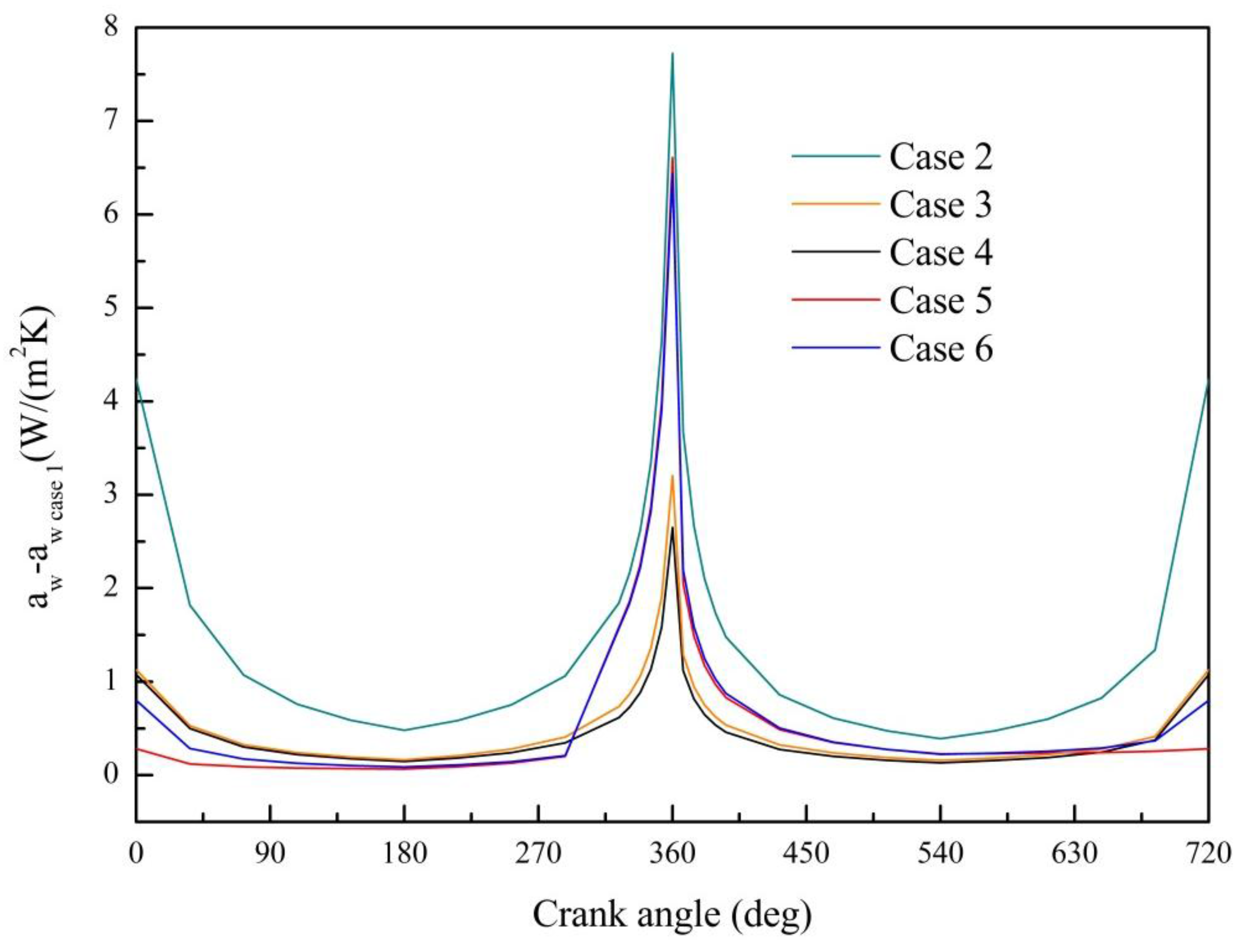
Differences in heat transfer coefficient between each case (Cases 2–6) and baseline (Case 1) are drawn in a complete cycle of 720° CA (crank angle) (Figure 7). It is shown the heat transfer coefficient is increased with the increase of inlet temperature, and the same effect can be found when the rated flow of coolant is changed in different strokes. Compared with changing the coolant flow, variation in the inlet temperature can achieve a much bigger increment in heat transfer coefficient. Increasing the rated flow of the compression and power strokes (Cases 5 and 6) can obtain higher heat transfer coefficient than Cases 3 and 4 Additionally, the rated flow of coolant in Stroke 2 and Stroke 3 have greater effect on the heat transfer coefficient than that in Stroke 1 and Stroke 4, and the beneficial effect seems to be negatively related to the increment of flow.

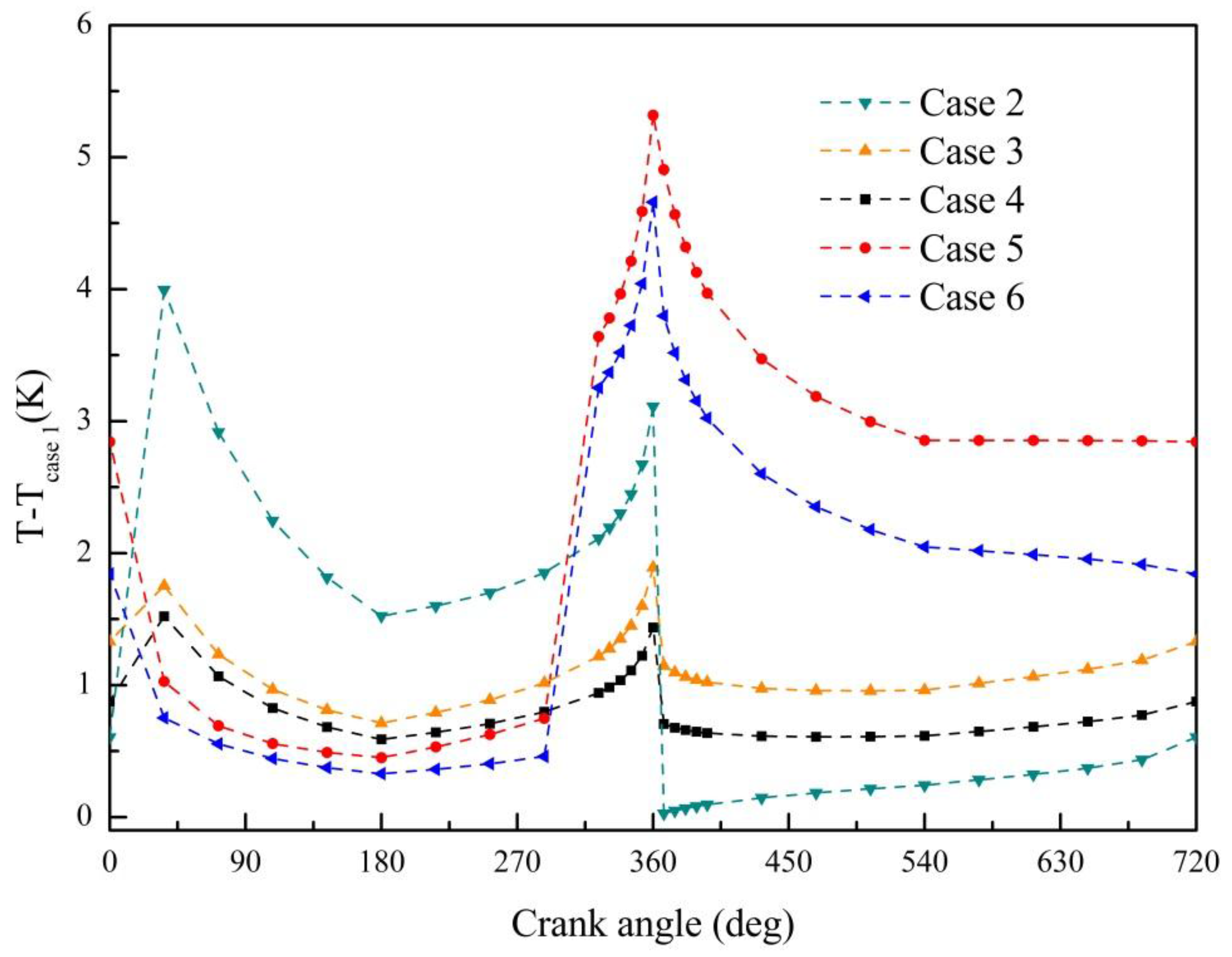
4.2. In-Cylinder Temperature

Differences in the in-cylinder temperature between each case (Cases 2–6) and baseline (Case 1) are drawn in a complete cycle of 720° CA (Figure 8). Taking the baseline case as reference, all the other five cases can obtain higher in-cylinder temperature if the coolant flow or the inlet temperature is changed. To increase the coolant flow in Strokes 2 and 3 (Cases 5 and 6) can result in much higher in-cylinder temperature increments compared with other cases. A smaller increment in coolant flow (Case 5) will lead to a higher increment in in-cylinder temperature. Controlling the inlet temperature can reach a considerable increment in in-cylinder temperature as well. In particular, the increment of in-cylinder temperature by rising the inlet temperature is apparently higher than that by changing the coolant flow before combustion, while that after combustion is the smallest. Increasing the coolant rated flow of the intake and exhaust strokes (Case 3) or decreasing that of the compression and power strokes (Case 4) increases the in-cylinder temperature very slightly.

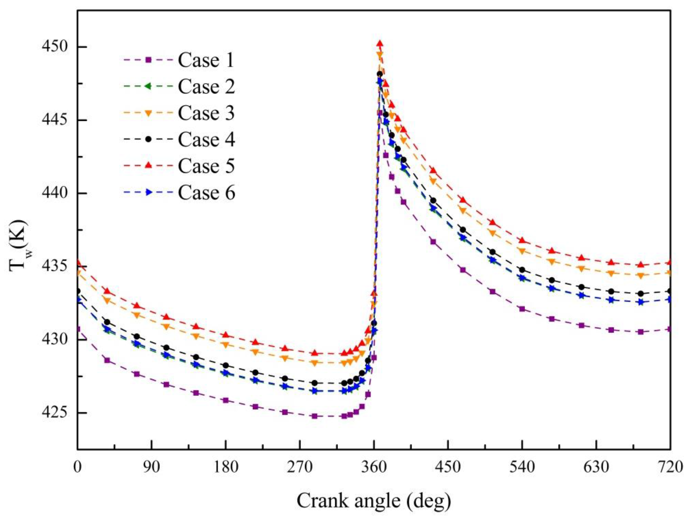
4.3. Average Wall Temperature

In Figure 9, the average wall temperature changes by about 20 K in all cases in a cycle and reaches a peak when the power stroke begins. Similar to the heat transfer coefficient and the in-cylinder temperature, increasing the coolant flow of the compression and power strokes by 50% (Case 5) can get the highest average wall temperature. However, the increment of average wall temperature of Case 6 is the smallest except the baseline case. In case 6, the increases of heat transfer coefficient and in-cylinder temperature are both the second highest. Instead, increasing the coolant flow in the intake and exhaust strokes leads to the second highest increase of average wall temperature.

4.4. Wall Heat Loss

Differences in wall heat flux between each case (Cases 2–6) and baseline (Case 1) are drawn in a complete cycle of 720° CA (Figure 10). Except for the inlet temperature control case (Case 2), the wall heat losses of other cases are lower than the baseline value in the intake stroke. After that, increasing the coolant flow of the compression and power strokes (Case 5) can significantly promote the heat transfer to the gas near the first bottom dead center, while keeping the coolant flow of the intake and exhaust strokes higher than that of the compression and power strokes (Cases 3–4) can reduce the heat loss, especially near 360°. It can be concluded that increasing the coolant flow is beneficial to the heat dissipation and decreasing the coolant flow is good for thermal efficiency.

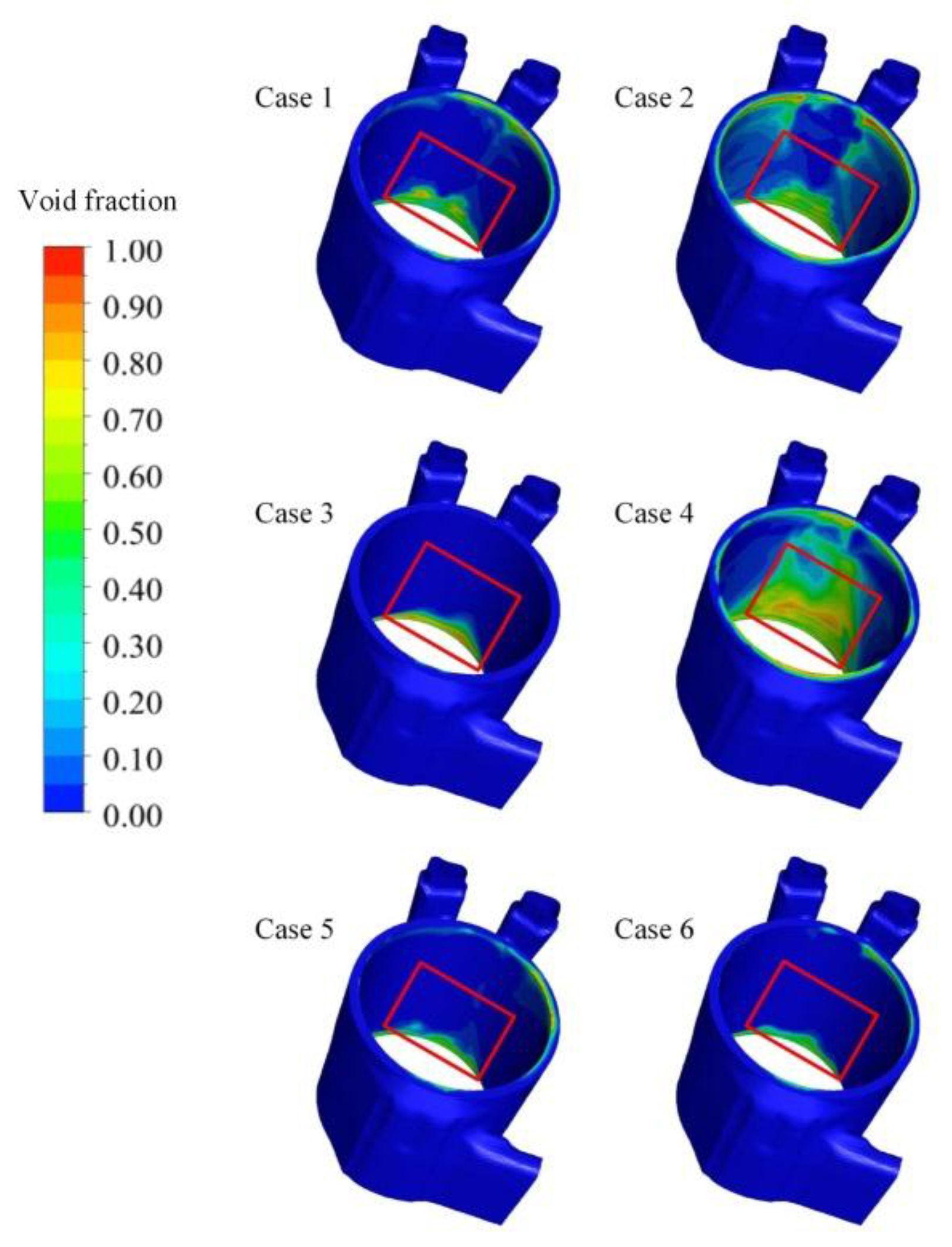
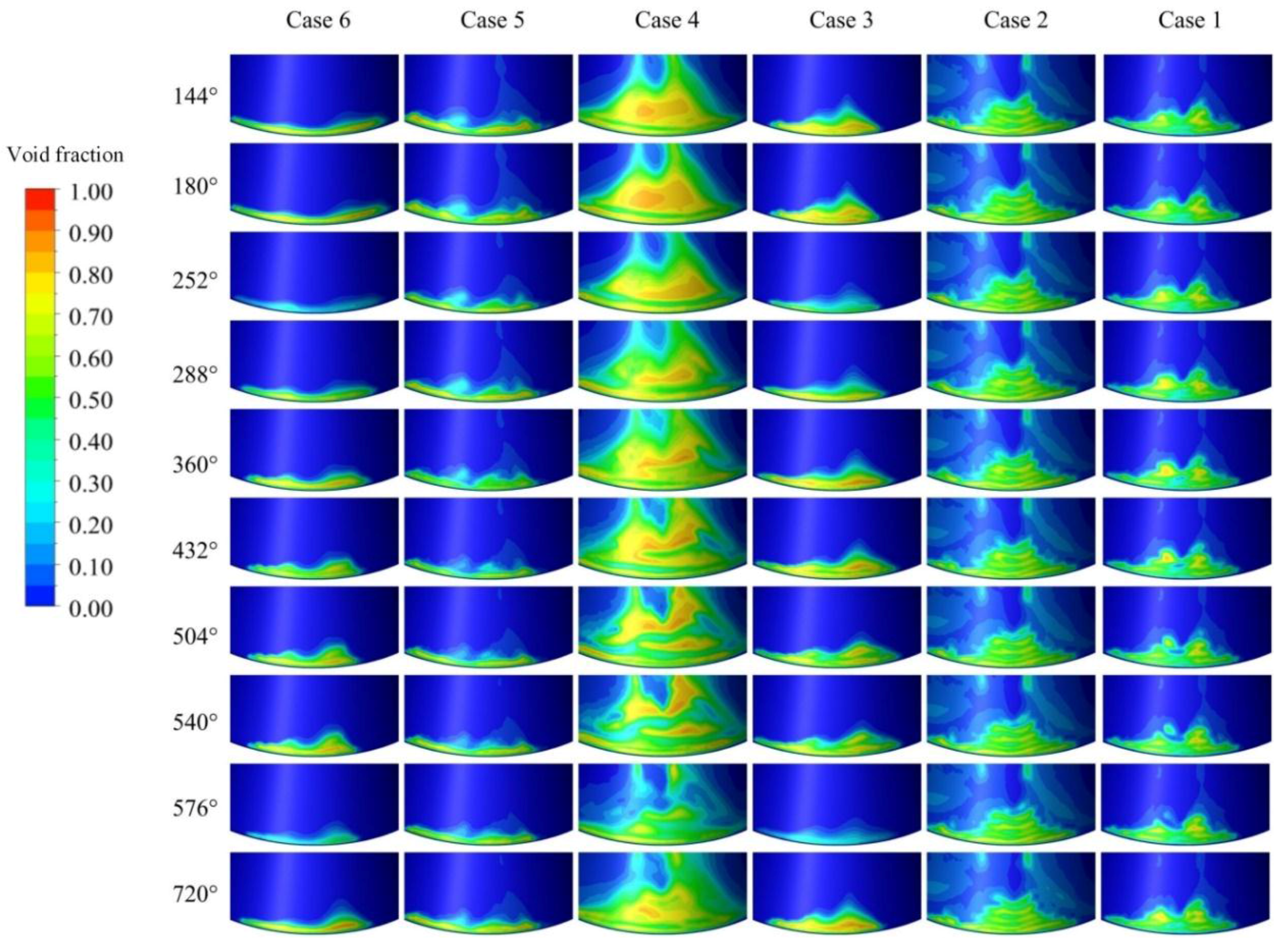
4.5. Gas Phase Distribution of Coolant

The gas phase distributions of coolant in different cases at different moments are given in Figure 11 and Figure 12. The color spectra represent the percentage of gas phase in the coolant. In most cases, the gas phase mainly concentrates on the outlet of the cylinder gallery. The top edge of the cylinder gallery on the outlet side also show gas phase concentration in some cases. In the baseline case, the gas distributions in all four strokes are quite similar, and those in the compression and power strokes are slightly higher than the intake and exhaust strokes. When the inlet temperature increases, more gas phase appears in the coolant, on the top edge of the cylinder gallery in particular. When the coolant flow of the intake and exhaust strokes is increased (Cases 3), the gas percentage in coolant decreases apparently especially for the top edge of the cylinder gallery. On the contrary, the decrease of coolant flow in the compression and power strokes (Cases 4) leads to significantly increase of gas phase in coolant. On the outlet side, about half of the gallery has more than 50% gas phase within coolant. Increasing the rated flow of coolant in the compression and power strokes (Cases 5 and 6) can greatly reduce the gas phase in the whole gallery. The gas phase distributions of the four strokes are also quite stable, and very small area of the cylinder gallery has relatively high gas phase in coolant. In the power stroke, the increase of flow reduces the gas phase slightly as shown from 360° CA to 432° CA in Figure 12. It is because the influence of increased coolant flow on the gas distribution is higher and covers the effect of the high heat flux. Comparing with Case 6, a lower coolant flow rate (Case 5) brings a higher gas phase distribution, especially in the intake and exhaust strokes. The variation of flow rate causes a retardation effect from the inlet to the cylinder wall, which leads to a minimum of gas phase around the bottom dead center, as shown from 252° CA to 576° CA in Figure 12. The reason is that near the bottom dead center of the intake stroke the gas in the coolant condensates and transfers heat to the in-cylinder gas. At the bottom dead center of the power stroke, the cylinder wall is still heating the coolant, the gas phase variation is positively related to the in-cylinder heat transfer coefficient due to the comprehensive effect caused by the heat flux changes and the multiphase heat transfer.

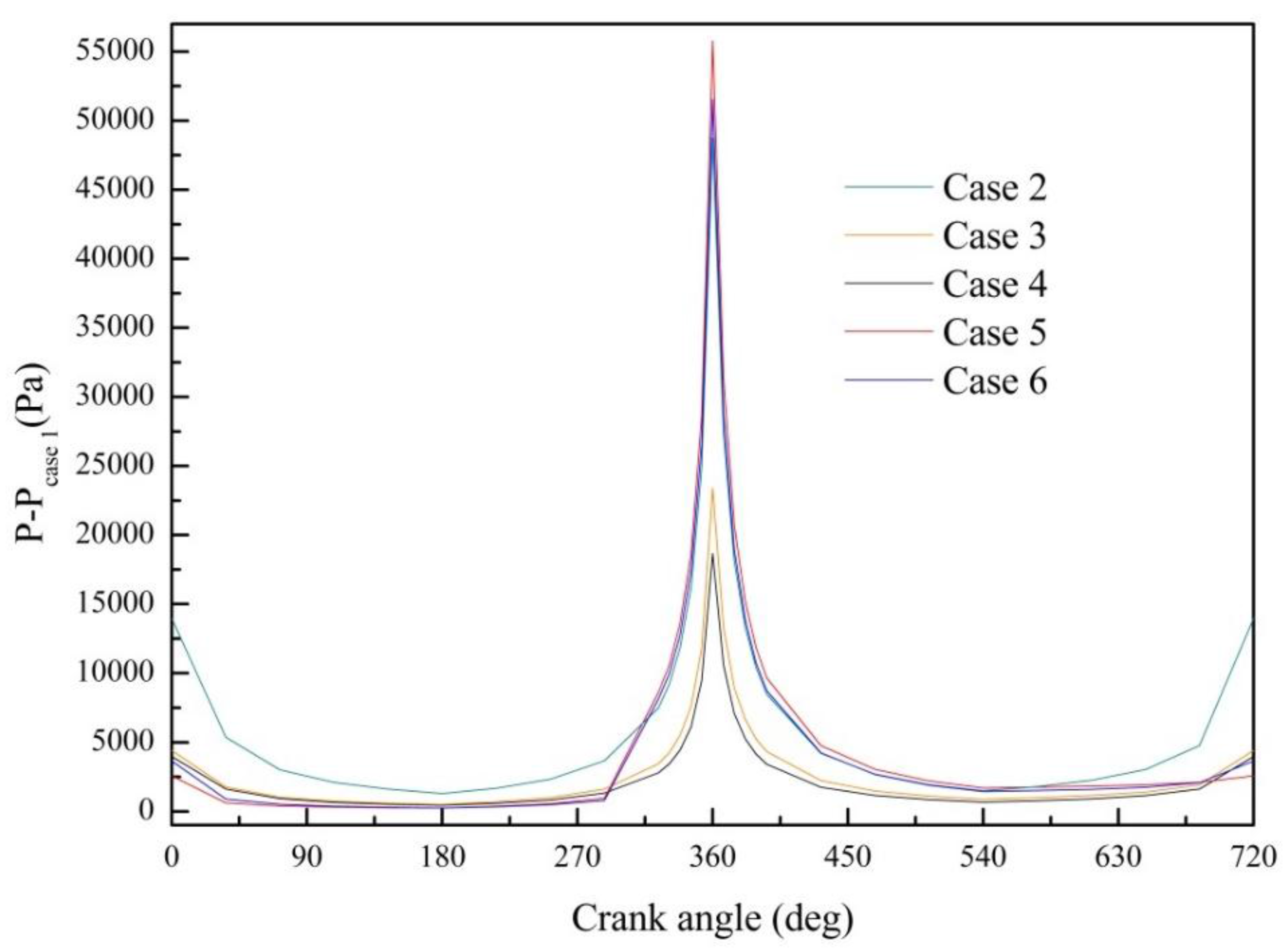
4.6. In-Cylinder Pressure

Differences in in-cylinder pressure between each case (Cases 2–6) and baseline (Case 1) are drawn in 720° CA (Figure 13). Controlling the inlet temperature (Case 2) is the only way to enhance the in-cylinder pressure in a whole working cycle. The control of the coolant flow is only able to increase the in-cylinder pressure around the combustion moment. The greatest increase (around 50 KPa) in peak in-cylinder pressure can be achieved by increasing the coolant flow of the compression and power strokes. Besides, rising the inlet temperature can also apparently increase the peak pressure as well.

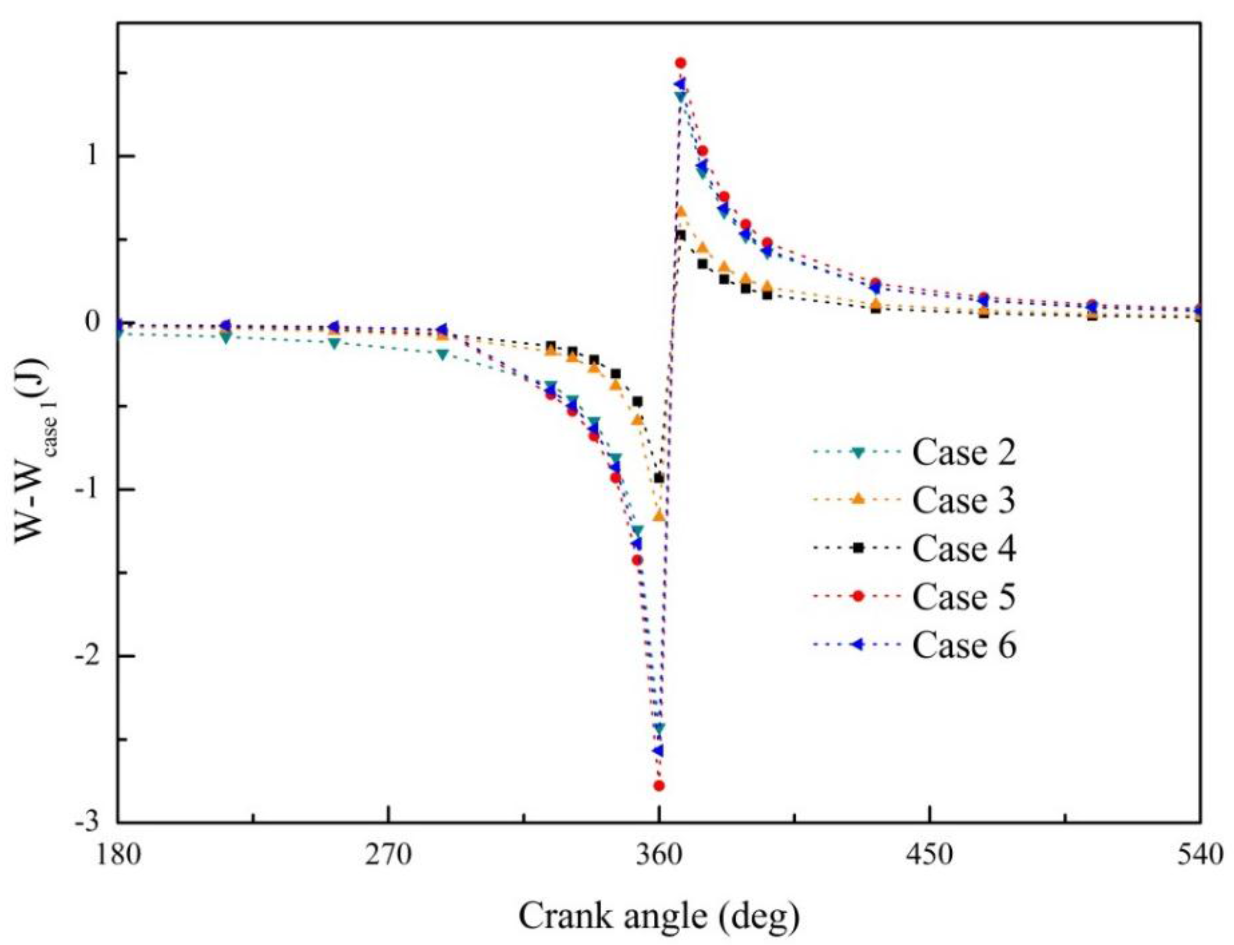
4.7. Engine Work

Differences in engine work between each case (Cases 2–6) and baseline (Case 1) are drawn in Figure 14.

The increase in in-cylinder pressure at the end of the compression stroke due to changing the control variables causes the increasingly negative work of engine. After that, the increase in pressure starts to provide beneficial effect on the engine work continuously. Among the five control cases (Cases 2–6), increasing the coolant flow of the compression and power strokes (Cases 5 and 6) can lead to the highest negative and positive engine work at the same time. Comparing with the inlet temperature-control case (Case 2), although the peak negative work of Case 5 and Case 6 is higher, the two coolant flow-control cases can lead to higher positive work at the power and exhaust strokes, even for the intake and compression strokes they would result in a lower total negative work.

The four coolant flow change schemes (Cases 3–6) use the top or bottom dead center as the starting point for the flow rate change. The coolant flow rate change delayed produces a change in engine thermal characteristics. It can be expected that if the flow rate is changed only in the vicinity of the combustion stroke, only the positive work of the gas in the cylinder increases. The coolant flow change time is determined by changing the flow rate, and the negative work can be minimized. This paper is focusing on the study of the thermal characteristics law of cooling variation based on the coolant rated flow scope, and has not explored the greatest benefits. The more exaggerated flow changes may bring the better returns.

4.8. Application Method Prediction

According to the changing laws discussed, effective intelligent control design of the engine can be performed. Taking into account the low accuracy of the coolant temperature monitoring, other parameters such as the in-cylinder pressure can be monitored based on the above-described changes in the engine's other thermal characteristics. The preliminary idea of a method for realizing such a pulse-like flow variation in each working cycle is to add a mechanical open-close flow device (such as a cam) on the basis of the original engine water pump or another auxiliary cooling circuit, according to the relationship between the flow rate change and the engine speed. This increases or decreases the stable coolant flow for a period of time in each cycle. Regardless of the cost of the device, only increasing coolant flow rate in the combustion stroke can be applied to high torque engineering work due to the higher maximum in-cylinder pressure and engine torque.

5. Conclusions

A modelling scheme for the coupling process of engine cooling and combustion is proposed by combining 1-D in-cylinder model and 3-D nuclear boiling model. The coupling simulation is carried out by exchanging information of in-cylinder temperature and heat transfer coefficient in every iteration. The detailed effects of cooling parameters on engine performances are obtained in working cycle level. Main conclusions drawn are as follows:

(1)

Increasing the coolant flow in compression and combustion strokes can significantly improve the in-cylinder gas temperature. The decrease in coolant flow in compression and combustion strokes can reduce the heat loss.

(2)

Reasonable increasing the coolant flow can achieve high wall and in-cylinder temperatures and low heat loss at the same time.

(3)

If the rated flow is decreased, the coolant with lower gas phase fraction can benefit the output power more. If the rated flow is increased, the coolant with higher gas phase fraction can improve the output power more. Proper design of coolant flow change time can maximize positive work without increasing negative work.