Assessment of Energetic, Economic and Environmental Performance of Ground-Coupled Heat Pumps


Department of Environment, Land and Infrastructure Engineering, Politecnico di Torino, Corso Duca degli Abruzzi 24, 10129 Torino, Italy
*
Author to whom correspondence should be addressed.
Energies 2018, 11(8), 1941; https://doi.org/10.3390/en11081941
Submission received: 15 June 2018
/
Revised: 17 July 2018
/
Accepted: 24 July 2018
/
Published: 26 July 2018
(This article belongs to the Special Issue Geothermal Energy: Utilization and Technology 2018)
Abstract
:Ground-coupled heat pumps (GCHPs) have a great potential for reducing the cost and climate change impact of building heating, cooling, and domestic hot water (DHW). The high installation cost is a major barrier to their diffusion but, under certain conditions (climate, building use, alternative fuels, etc.), the investment can be profitable in the long term. We present a comprehensive modeling study on GCHPs, performed with the dynamic energy simulation software TRNSYS, reproducing the operating conditions of three building types (residential, office, and hotel), with two insulation levels of the building envelope (poor/good), with the climate conditions of six European cities. Simulation results highlight the driving variables for heating/cooling peak loads and yearly demand, which are the input to assess economic performance and environmental benefits of GCHPs. We found that, in Italy, GCHPs are able to reduce CO2 emissions up to 216 g CO2/year per euro spent. However, payback times are still quite high, i.e., from 8 to 20 years. This performance can be improved by changing taxation on gas and electricity and using hybrid systems, adding a fossil-fuel boiler to cover peak heating loads, thus reducing the overall installation cost compared to full-load sized GCHP systems.
1. Introduction
Heating, ventilation and air cooling (HVAC) of buildings account for 30–40% of global energy demand [1,2,3] and approximately 30% of energy-related greenhouse gas (GHG) emissions [2]. For this reason, introducing low-carbon technologies in this sector is vital for the fight against climate change. Geothermal heat pumps (GHPs), which exploit shallow ground as a heat source or sink, are one of the least carbon-intensive HVAC technologies [4,5]. Compared to air source heat pumps, they are more efficient, since the ground has a stable temperature which is usually warmer than air during winter and cooler during summer. GHPs can exchange heat with groundwater (groundwater heat pumps, GWHPs) or by circulating a water-antifreeze mixture through pipe loops buried into the ground (ground-coupled heat pumps, GCHPs). The most common GCHP technique is the borehole heat exchanger (BHE), composed of one or two U-pipes installed in an expressly drilled small borehole filled with a special grout, reaching depths between 50 and 100 m [6]. While GWHPs need a thick and productive aquifer, BHEs can be installed almost everywhere. Recent projects have highlighted the role of ground properties on the economic feasibility of BHEs [7,8], but they did not take into account a detailed usage profile of the heating and/or cooling system, which is also very influential for their economic return. The main drawback of BHE systems is their high cost and, thus, an accurate assessment of thermal loads and their time trends is vital to avoid under- or over-sizing of GHPs. The best approach to fulfil this task is dynamic energy simulation, integrating the building and the HVAC system (i.e., BHEs, heat pump, storage, distribution network, and heating/cooling terminals) [9]. The TRNSYS (TRaNsient SYstem Simulation tool) (Thermal Energy System Specialists, LLC, Madison, WI, USA) suite is one of the most used dynamic energy simulation tools. It is based on modular components called Types, which reproduce devices (e.g., a heat pump, a boiler, a PV panel, a pump, and a heat exchanger) and external driving forces (e.g., climate and shading), allowing to link them through input and output variables [10,11].
Numerous studies on GCHPs have been conducted with TRNSYS [12,13,14,15,16,17,18,19,20,21,22,23,24,25,26,27,28,29,30,31,32]. The importance of using short time steps (even sub-hourly) to allow a realistic system sizing has been stressed in Ref. [12]. The integration of solar thermal and PV systems with GHPs was studied in Refs. [13,14,15,16]. Studies on GCHPs applications in European [17,18,19,20,21], American [22,23] and Asian climates [24,25] have been performed, in single residential or office building cases. Analyses of economic feasibility and environmental benefits for residential buildings were carried out by Lu et al. [26], Morrone et al. [27], and Chang et al. [28]. Ciulla et al. [29] estimated the thermal energy demand for the office building typology in different European climates. Moreover, Junghans [30] studied the effect of thermal insulation on the profitability of geothermal systems. The hybrid gas boiler–GCHP configuration, i.e., plants where peak heating loads are partially covered by a gas boiler, was studied as a mean to reduce the overall installation costs of GCHPs in Refs. [31,32].
The aforementioned studies separately examined technical, economic and environmental aspects of GCHPs in different contexts, but a comprehensive analysis of these factors is missing, in particular for the hybrid–GCHP configuration. This paper fills this gap through the analysis of the results of a series of dynamic TRNSYS simulations on benchmark buildings of three different typologies (detached house, office building and hotel), two degrees of thermal insulation, and six climate datasets representative of all Europe. The building energy model developed in TRNBuild allowed the sizing of the heat pump–BHE system and the subsequent integrated simulation of building and HVAC system with the TRNSYS suite. The results of these simulations were processed to derive indicators for the energy, economic and environmental performance of GCHPs in different contexts. Peak loads and yearly heating/cooling needs for different building typologies and different climates are analyzed and their influence on the economic convenience of GCHPs is assessed through indicators such as discounted payback period (DPP), net present value (NPV), and internal rate of return (IRR). The influence of incentives is also quantified, considering current Italian schemes. Since the initial investment proved to be a relevant barrier, the use of different hybrid heat pump–gas boiler configurations is also evaluated to reduce the installation cost of GCHPs. The reduction of greenhouse and pollutant emissions is finally estimated, assessing the cost-effectiveness of GCHPs from the environmental point of view.
2. Methods
The operation of GCHP systems in different building typologies and climates across Europe was simulated with TRNSYS 16.0. The build-up of models and the modeling assumptions are described in this Section, with further explanation and data in the Supplementary Materials.
2.1. Buildings and Climatic Conditions Simulated
A total of 36 models were developed considering combinations of:
- -
- Three different building types, i.e., a single family detached house (House), a small two-story office building (Office) and a multi-story hotel (Hotel). Data on their size are reported in Table 1. Each building destination is characterized by a different occupancy level, air change schedule, temperature setpoint and use of the HVAC system, as described in Section 2.2.
- -
- -
- Two thermal insulation levels: “good” insulation, in compliance with the present Italian legislation (see Ref. [34]), and “poor” insulation, representative of buildings of the 1960s using reference values from TABULA project [35]. The thermal transmittance values of building envelope are reported in Table 2 for opaque elements and in Table 3 for windows. Details on the layers constituting the opaque elements are available in the Supplementary Materials (Section 1.1, Tables S1–S8).
2.2. The Building-HVAC Model
The main subdivision of the TRNSYS model is between the building and the other subsystems as shown in Figure 2.
Type 56 (building) is the central component of the TRNSYS global model, which receives the external weather conditions as input, determines the thermal balance, and delivers the internal conditions to the thermostat/humidistat [37]. Consequently, the thermostat controls the distribution components to maintain the desired indoor temperature and humidity previously set in the schedules. The distribution system is composed of fancoils and an air handling unit (AHU), which work exchanging heat between the air inside the building and the water circuit. The heat pump (HP) heats (or cools) the water of the distribution system and thus supplies energy to the fancoils, the AHU, and the Domestic Hot Water (DHW) systems. A buffer tank is placed between the HP and the distribution system, to ensure the correct operation of the HP, reducing the frequency and increasing the length of its operating cycles. In the hybrid system cases, the heat pump is assisted by a gas boiler. Finally, the HP exchanges heat with the ground through the BHEs.
2.2.1. Building
The building was defined in Type 56, identifying the different zones and providing input data such as wall and window stratigraphy, shading schedules and internal gains.
Type 56 solves the thermal balance of the different thermal zones of the building, lumped into “air nodes” representing the air volume inside them. The air node receives a heat input (W), which is the sum of the convective heat flow (W) from all inside surfaces (walls), the infiltration gains/losses (W), the ventilation gain (W) from sources such as a heating/cooling terminal, the internal gains (people, equipment, etc.), and a coupling term (W) representing the air flow from neighbouring thermal zones (further details in Ref. [37]):
where (°C) is the temperature of the “air node”, (W m2 K−1), (m2) and (°C) are, respectively, the transmittance, the area and the external temperature of the i-th wall, (J m−3 K−1) is the thermal capacity of the air, (m3 s−1) is the infiltration volumetric flow rate, (°C) is the outdoor temperature, (m3 s−1) is the ventilation volumetric flow rate of the i-th ventilation component, (°C) is the air temperature of the i-th ventilation component, (m3 s−1) is the air volumetric flow rate coming from the i-th bounding zone, and (°C) is the air temperature of the i-th zone.
The House and Office buildings were divided into the heated/cooled space and the attic (with no thermal regulation); the Hotel, instead, was divided into first (i.e., lobby/reception and restaurant) and upper floors (i.e., the rooms) with different occupancy levels and ventilation requirements.
The occupancy level, which influence internal gains and aeration, were set as follows:
- -
- The House hosts 4 people from 4:00 p.m. to 8:00 a.m. on working days, and all day on weekends.
- -
- The Office hosts 20 people during working hours (8:00 a.m. to 4:00 p.m.).
- -
- The Hotel hosts a maximum of 28 and 112 people, respectively, during low and high season. Further details on the occupancy level of the Hotel are shown in Table S9 of the Supplementary Materials [38].
Weather data such as solar irradiation and air temperature were provided by Type 109, based on the Meteonorm database [36].
2.2.2. Thermostat and Schedules
The five-stage thermostat (Type 108, see Ref. [39], page 33) and the on-off humidistat (Type 658, see Ref. [40]) evaluate the building inner conditions (air temperature and humidity) and control the distribution system operation in order to keep the room temperatures and relative humidity values within the following ranges:
- -
- Temperature: 20 ± 1.3 °C in winter and 26 ± 1.3 °C in summer for the House and Office buildings. The Hotel has more demanding setpoints, i.e., 22 ± 1.3 °C in summer and 25 ± 1.3 °C in winter.
- -
- Relative humidity: 50 ± 10% for all building types.
The temperature regulation is performed by the heating and cooling system, while the relative humidity control is used to adjust the internal air change rate, which is calculated depending on the building type according to Ref. [41] (see Section 1.3 of the Supplementary Materials). The setpoints have to be respected during the scheduled time ranges reported in Table 5.
The dead band around the temperature (±1.3 K) and relative humidity (±10%) setpoints was defined to reduce the frequency of on-off cycles of the fan coils (Section 2.2.3) of the heat pump. A setback temperature was set in the heating season for the House (18 °C) and Office (15 °C), as suggested by Rable and Norford [42], to soften the start-up of the heat pump at the beginning of the scheduled times (see Table 5). No setback is set for the Hotel since thermal regulation is always on.
2.2.3. Distribution and Terminals
The distribution system is composed of the fancoils and the AHU, and it is controlled by the thermostat and the humidistat. The fancoils work with a water temperature of 50 °C in heating conditions and 12 °C in cooling conditions. Type 752 for cooling (see Ref. [40]) and Type 754 for heating (see Ref. [40]) were chosen to control the room temperature by modulating the air flow rate according to the internal conditions. Inside the fancoils, air is heated or cooled by 7 K relative to the building temperature [43], while water inside the coils is cooled by 10 K in heating conditions, and heated by 5 K in cooling mode. Air change and humidity level are controlled by the AHU (Type 696, see Ref. [40]), except for the House, where air changes are adjusted manually and no humidity control is provided.
2.2.4. Buffer Tank
The buffer tank (Type 4, see Ref. [39], page 347) is a stratified reservoir of hot water in winter and of cold water in summer, connected to the heat pump circuit and the distribution system. Inlet and outlet pipes are arranged to preserve water stratification; thus, their position is switched from summer to winter. Two aquastats (Type 502 for heating season and 503 for cooling season, see Ref. [40]) control the water temperature inside the tank, activating the heat pump when the temperature of the water flowing to the distribution system drops below 50 °C (heating season) or exceeds 12 °C (cooling season) [43]. Furthermore, a dead band of ±2 K was applied to the aquastat. The tank volume is set to 25 L per kW of HP capacity according to Ref. [44].
2.2.5. Heat Pump and Auxiliaries
The water-to-water heat pump is simulated with Type 668 (see Ref. [40]), which interpolates the values of thermal power delivered and the electrical power consumed (and, hence, the COP) from a number of values determined at specific source and sink temperatures, derived from technical sheets of commercial HPs with different peak heating/cooling power [45,46]. An example is shown in Figure 3 for a heat pump with 10.5 kW of heating peak power.
The HP size was first determined equal to the steady-state thermal power exchanged by the building at heating design temperature, in the absence of any solar or internal heat gains [41]. The design outdoor temperatures values are 0.4% quantiles, as suggested by ASHRAE [45] and are reported in the Supplementary Materials (Table S10, Section 1.4). This kind of evaluation could not be performed for the cooling needs, which depend on the gains and irradiation. Therefore, the cooling peak load was estimated by trial-and-error, and the heat pump capacity was finally sized based on the largest between heating and cooling peaks. After this pre-sizing phase, a yearlong simulation was conducted to derive the heating and cooling load curves.
2.2.6. Domestic Hot Water
The domestic hot water (DHW) is provided by the tap water circuit and a specific buffer tank (Type 60, see Ref. [39], page 367) that exchanges heat with the HP water circuit through a copper coil. The DHW usage profiles differ for each building type, with daily consumption per capita defined by the Italian UNI TS 11300 part 2 [46]. The Office usage profile was assumed to be equally distributed during working hours, while a report by Jordan and Vajen [47] was used for the House and Hotel. The water is heated up to 60 °C inside the tank and then mixed with cold water from the main until it reaches 45°C, as suggested by Ref. [46].
In the case of concurrent ambient cooling and DHW needs, the HP can switch the heat exchange with the condenser from the borehole heat exchangers to the hot water tank circuit [9].
An anti-legionella cycles is also scheduled based on Ref. [41].
2.2.7. Borehole Heat Exchangers
Borehole heat exchangers (BHEs) are included in Type 557 and based on the Duct Ground Heat Storage Model (DST) developed by Hellström [48]. The borehole field was sized with the ASHRAE method [49,50]:
where (m) is the borehole total length; (°C) is the average fluid temperature; (°C) is the undisturbed ground temperature (here assumed equal to the yearly average air temperature); (°C) is the temperature penalty due to reciprocal interference between BHEs (a model is provided in Ref. [49]); , and (W/m) are the annual mean, the peak monthly and the peak hourly values of the thermal load exchanged with the ground, respectively; , , and (mK/W) are the respective values of the thermal resistance of the ground; and (mK/W), assumed equal to 0.109 mKW−1 [19], is the borehole thermal resistance.
This equation should be applied considering both the heating and the cooling function. Two different lengths (, ) are derived, and the highest value is selected.
Thermal loads (, , ) were extracted from the system simulation; monthly () and hourly () loads for the calculation of heating () and cooling () BHE lengths are different, while is the same and was derived from the yearly thermal budget between heating and cooling.
The BHE field was first sized with Equation (6) using the thermal loads calculated in the heat pump sizing procedure, i.e., without including the components of the HVAC system but considering an ideal one, which adapts the indoor temperature instantaneously to the set point/setback. This first estimate was used as an input for Type 557 in the complete TRNSYS model to derive thermal load curves to be used as an input for a second BHE sizing with Equation (6). The process was repeated until the length difference between two iterations became negligible and the final length was rounded to realistic BHEs installation lengths (of 80, 90, 100, 110 or 120 m).
2.2.8. Backup Gas Boiler
In hybrid systems, a condensing gas-fired boiler (Type 700, see Ref. [40]) was placed in the water circuit after the buffer tank. In the case of heating load exceeding the HP capacity, the boiler switches on and delivers a user-defined thermal power at a fixed efficiency (assumed equal to 97% based on Refs. [41,46]).
The hybrid system was sized based on the correlation between the HP load factor and the total energy demand met (TEDM) by the GCHP [32], derived from the load time series generated by the building model (explained later in Section 3.2.1). For each model case, either a 90% or a 70% energy demand coverage by the heat pump was assumed, while the remaining peak demand was assumed to be covered by the gas boiler. The HP power was consequently reduced according to the load factor corresponding to the TEDM value adopted, while the boiler power was set to equal the HP power in the GCHP-only case.
3. Results and Discussion
The results of the simulations provide insights on energy demand, which can be used as an input for economic and environmental analyses. Section 3.1 presents the resulting energy demands and peak loads, both for heating and cooling. The results of plant sizing and of energy demand were used to estimate the installation and operational costs, and hence to assess the economic feasibility of shallow geothermal energy, with a focus on the Italian situation (Section 3.2). Finally, the environmental benefits are assessed, estimating the reduction of fossil fuel use, of CO2 emissions and of air pollution (Section 3.3).
3.1. Energy Consumption
The peak heating/cooling loads and the energy demand are the key input parameters for sizing the HVAC components. To make results comparable among buildings of different size, results are shown in Figure 4 as heating/cooling peak loads per unit area (W/m2). Heating loads are generally higher than cooling ones in European climates, especially in poorly-insulated buildings. This is the case of the Office building (Figure 4A,B), with values 30% to 130% higher than the other building types due to the Monday morning start-up, and of the high cooling loads (up to seven times the Hotel loads, Figure 4C,D) due to the high internal gains. The Hotel has lower peaks since the HVAC system operates with a longer schedule (see Figure 4) due to higher comfort standards. A better thermal insulation reduces heating loads by about 50–70% and, in warm climates, also cooling loads. On the other hand, it slightly increases cooling loads in cold climates, as the internal gains increase their relevance in the heat budget, especially in the Office case. With a good insulation, the difference between heating and cooling peaks diminishes (especially in Zones B and D) thus allowing for a better exploitation of the reversible heat pump.
The energy demand for heating and cooling is expressed per unit area (kWh/m2/year) and is closely correlated to the heating (Figure 5A,B) and cooling (Figure 5C,D) degree days, thus confirming the validity of the heating/cooling signature approach [51].
Similar to the thermal loads, the energy demand is strongly influenced by the thermal insulation, and switching from poor to good insulation can reduce it by 70–90%. The heating signatures of poorly insulated buildings (Figure 5B) are of course characterized by steeper slopes, as well as by a higher intercept, since building heating is required even in warmer conditions. The energy signature of the Hotel has a gentler slope due to the smoothing effect of the uninterrupted schedule but, at the same time, the higher comfort requirements determine a high intercept, because heating is switched on at warmer conditions to cope with a higher setpoint compared to the other buildings. The well-insulated Office requires some cooling even in the coldest climates with low or zero CDD (Figure 5C), due to the high internal gains. On the contrary, the House typology has relatively low cooling needs due to the low occupancy in the warmest hours of the working days.
The heating demand (Figure 5A,B) depends more on climate compared to the peak heating load (Figure 4A,B): the ratio between these quantities is the number of full-load equivalent operation hours (FLEH) and indicates how intensely is a heating (or cooling) plant used. Zones A and C have both a low heating demand and low FLEH, which limit the economic feasibility of installing a GCHP (Section 3.2). A small difference between the annual heating and cooling demand is highly desirable, since it reduces the long-term thermal alteration of the ground, and it is observed mostly in well-insulated cases in the climate Zones B and D. In the other cases, the heat budget unbalance induces a ground thermal drift, reducing the system performance over time.
Domestic Hot Water (DHW) is not considered in the heat pump sizing, because it is stored and not produced instantaneously, and hence the required power is much lower than any building peak heating load. However, the energy demand for DHW may represents up to 80% of the consumption in well-insulated buildings in warm climate zones, due to the low heating needs. In the other cases, its value ranges between 24% and 1% of the total heating demand.
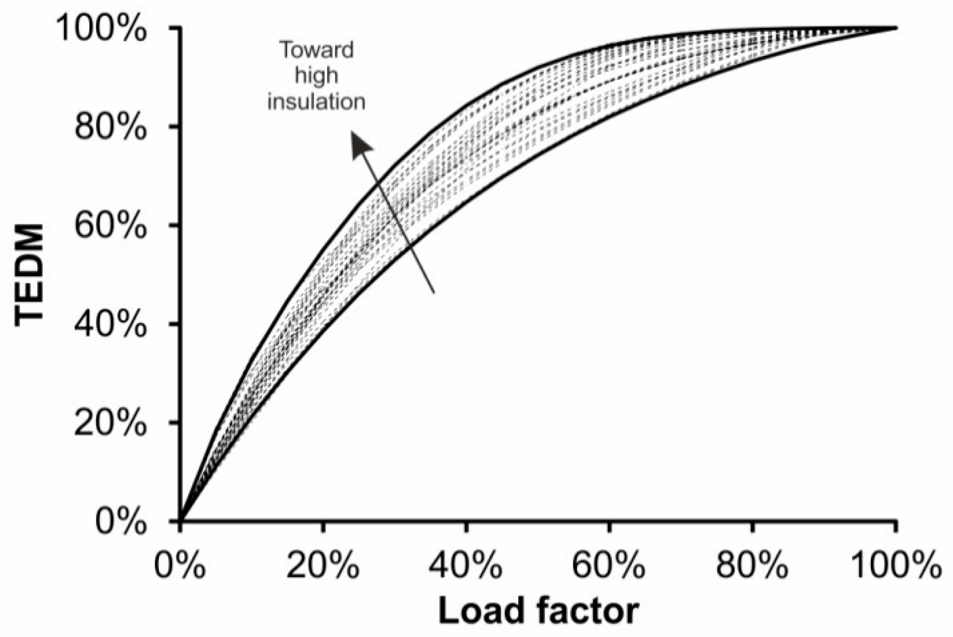
The time series of heating and cooling load allow to derive cumulate distributions, such as the one shown in Figure 6, which correlates the load factor of the heat pump with the total heating/cooling demand met (TEDM), on an hourly basis. The results of all simulations are comprised among the thick black lines. For example, a heat pump sized at 60% of the peak load is able to meet 82–96% of the total yearly heating demand, consistent with a few previous studies [31,32,52].
In the hybrid cases analyzed below, the HP is installed to cover the base demand, while a backup system is used to manage the peaks. The plot shown in Figure 6 can be used for sizing the HP and the auxiliary boiler at different shares of TEDM.
The installation cost of the system with a hybrid configuration can significantly be cut due to the reduced HP capacity and BHE length. Additionally, a reduction of the frequency of on–off cycles is achieved, which could extend its operating lifetime [43].
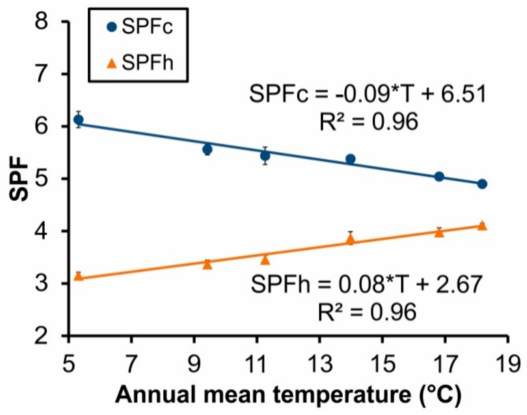
The efficiency of the HP strongly depends on climate and it is usually expressed by the seasonal performance factor (), i.e., the load-weighted average COP during heating () or cooling () seasons. As shown in Figure 7, the heat pump performs better for heating in warmer climates, while the opposite occurs for cooling. This behavior is attributable to the undisturbed ground temperature (here assumed equal to the annual mean air temperature).
Of course, as the underground temperature can be locally altered (e.g., by geothermal gradients) these conclusions may not apply in all cases.
3.2. Economic Performance
To compare a conventional heating/cooling system and a GCHP system, an economic analysis was carried out, considering either a new installation (in well-insulated buildings) or a replacement of the existing heating/cooling system (refurbishing of poorly-insulated buildings). This analysis allows distinguishing profitable investments from ineffective ones, based on three economic indicators: the net present value (NPV), the discounted payback period (DPP) and the internal rate of return (IRR) [53]. It is straightforward that, at least, NPV should be positive at the end of the evaluation period of the investment. The net present value is calculated as:
where (€) is the total investment cost, (€) is the operational saving granted by the GCHP compared to the conventional system over the plant lifetime, (€) is the difference between the total operation and maintenance cost difference of the GCHP and the conventional plant over their lifetime, (€) are the total subsidies supplied, is the discount rate, is the effective discount rate [53], (year) is the lifetime of the GCHP system (assumed equal to 25 years [54,55]), (year) is the number of years during which subsidies are provided.
The discount rate represents the cost of capital and was assumed equal to 2% as suggested by the European Central Bank [56]. The rate of increase of energy cost was set to 2% same as the discount rate but, of course, it can have different values. The installation cost, , is the sum of the components’ costs including installation labour and taxation.
The equipment required for both conventional and new plants were not considered in the analysis; thus, AHU and fancoils were assumed to be already installed in the Office and Hotel, and their installation cost was not calculated. Conversely, fancoils were considered, along with the GCHP installation, in the House refurbishment case, where they are supposed to replace high temperature radiators.
The capacity-cost curves for each piece of the system were built with data derived from commercial catalogues [57,58,59,60,61] and are reported in the Supplementary Materials (Table S15), while the BHEs drilling and installation cost were assumed constant and equal to 60 €/m [62]. After defining the components’ cost, the total investment cost of the plant was obtained by summing the single components’ costs and the labor cost for plant installation. Tax was added to the final cost considering the Italian taxation system (Value Added Tax, VAT) on the labor and equipment component of the installation costs [63]. VAT rates on equipment (normal rate) range between 18% and 27% in the EU-28 Member States [64], while different kind of rates could be applied to the labor costs.
The share of each factor contributing to the total cost of the system varies in the different cases. In the example of the 28 kW poorly-insulated House in Zone D, the total cost is distributed as follows: drilling and BHEs installation (44%), HP (19%), fancoils (9%), labor (6%), taxes (17%), and additional equipment (5%). In general, the cost related to boreholes represents the largest contribution to the total installation cost, with a logarithmic correlation with the BHEs total length installed as shown in the Supplementary Materials (Figure S4).
Data obtained from the simulation were processed to calculate the annual electrical energy consumed by the heat pump and the circulation pump of the BHEs. The energy required for both the conventional and the GCHP system was not considered in the analysis (e.g., distribution pump, AHU, etc.). The price for the energy resources were extracted from Eurostat data [65].
The annual revenue achieved with the installation of a GCHP was calculated as:
where and (kWh) are the building heating and cooling energy determined by the model simulation; and (€/kWh) are the natural gas and the electricity price, equal to 0.0719 €/kWh and 0.1818 €/kWh, respectively [66]; is the conventional non-condensing gas boiler efficiency, equal to 76% [41,46]; is the seasonal coefficient of performance of the conventional air conditioning system obtained from the model simulations (for each climate zone) and based on NREL tests [67]; and (kWh) is the electrical energy consumed by the system calculated through simulations, considering all the components related only to the GCHP (i.e., excluding the distribution and terminal auxiliaries, since they are also included in conventional HVAC systems).
The O&M costs represent the annual expenditures for ordinary maintenance of the plant and are calculated as the difference between the GCHP and the conventional system maintenance costs, based on Refs. [54,55,68].
Finally, two different scenarios were considered: absence of subsidies, which represents the case of a GCHP installation in a brand-new building, and the presence of subsidies, in the case of the refurbishment of an existing building. Subsidies were assumed equal to 65% of the total investment cost, refunded in ten equal yearly payments (), according to the Italian incentive scheme [63]. For this reason, while the evaluation on the unsubsidized case could be extended with a good degree of approximation to other EU countries, the subsidized case only applies for Italy.
The discounted payback period is the time required for the NPV to become equal to 0 [53], while the internal rate of return represents the discount rate for which the net present value is null at a certain period of time [69]. The calculated IRR corresponds to the one evaluated at the end of the plant life (i.e., after 25 years).
The GCHP system is profitable if IRR is sufficiently high, NPV is positive and DPP is not too long. According to Newnan et al. [69], 2% is the lowest acceptable IRR for investments in energy efficiency, but companies are more focused on the short term, and hence a higher IRRs are usually requested to opt for a certain investment [70]. Table 6, the feasibility of the different cases, with or without subsidies, is reported: in the case of negative NPV and IRR the system is not economically feasible; if the IRR is lower than the acceptable rate of return (2%), the investment should be carefully evaluated; finally, if the IRR is acceptable and the NPV positive the system installation is feasible.
In general, in the current European economic scenario, GCHP systems designed to cover the whole heating demand are unfeasible without public subsidies. Replacing an existing system in a poorly-insulated building is economically convenient due to the high energy consumption, which implies high possible revenues. This holds true in particular for hotels due to the higher number of operation hours per year. As shown in Figure 8, the discounted payback periods (DPP) are similar throughout the heating-dominated incentivized cases with a general decrease toward high energy-consuming buildings (i.e., scarce insulation cases and cold climates) and when the full load hours are maximized and the load curve is characterized by low peaks, because of both lower installation costs and higher operational savings. DPP of 9–13 years can be achieved in most of the refurbished buildings displayed in Figure 8. Among these, climate Zone B (in poorly insulated cases) presents balanced heating and cooling needs, and the shortest DPP (i.e., 8.6 years). Cooling-dominated buildings in Zones A and C are, instead, low energy-consuming, which results in very long payback periods. This is particularly true when subsidies are not available (generally the case for new buildings), with a minimum payback period of 16 years.
3.2.1. Hybrid System Results
The energy and economic analysis was extended to the hybrid cases. The building load curves were used to size the HP capacity to cover 90% or 70% of the annual heating demand, while the share is assumed to be covered by a gas boiler.
The estimation on load factor–TEDM curves such as in Figure 6 proved accurate for the House (Figure 9), with a slight underestimation of the TEDM by the backup system (3% average difference, see Table 7). By contrast, the predicted energy covered by the boiler was highly overestimated for the Office and the Hotel (13% difference on average, see Table 7), meaning that an ad hoc simulation process with a trial-and-error approach is required for sizing. The peak loads are reduced by the thermostat dead band and by the buffer tank, and, thus, the loads based on the building requirements are overestimated compared to the real ones.
These results suggest that an estimation of the hybrid backup system based on the building load curve is conservative for the Office and Hotel buildings, while it is correct in the House case as shown in Table 7. In the example of the poorly-insulated Hotel in Zone D (HP covering 100% of the peak load), the payback period is equal to 18.4 years without subsidies and 9.9 years with subsidies. When sized at 90% TEDM (54% load factor), the system actually covers 97% of the heating demand, with a payback time of 14.2 years without incentives (23% reduction) and 8.6 years with incentives (13% reduction). In the 70% TEDM sized case (36% load factor) the system actually covers 86% of energy demand, with a payback equal to 12.9 years without incentives (30% reduction) and 7.3 years with incentives (−26%). Summarizing, the introduction of a backup system can reduce the payback period of the system by up to 20–40% thanks to the reduction of the HP and BHE costs. The investment becomes profitable for the Hotel cases even without subsidies. Further studies should optimize the economic output of a hybrid system and provide a reliable estimation method based on the building load curve.
3.2.2. Electricity/Fuel Price Ratio Analysis
An additional analysis was conducted on the electricity/fuel price ratio and on its effects on the economic indicators. In general, the price ratio should be lower than the heat pump SPF/boiler efficiency ratio, otherwise no saving can be achieved on the operational costs. This request is always met in the simulated scenarios, since the lowest SPF/boiler efficiency ratio equal to 4.1 (poorly-insulated Hotel in Zone F) and the electricity/fuel price ratio (Table 8) never reaches such a high value. For this reason, the GCHP allows achieving some operational saving in all 36 cases analyzed. The ratio was evaluated in the base case of natural gas combustion (with and without the actual taxation share) in the Euro Area (EA) and in different countries (Italy, Germany, Spain, and France). A further comparison with heating oil and heating LPG [66,71] is made for Italy.
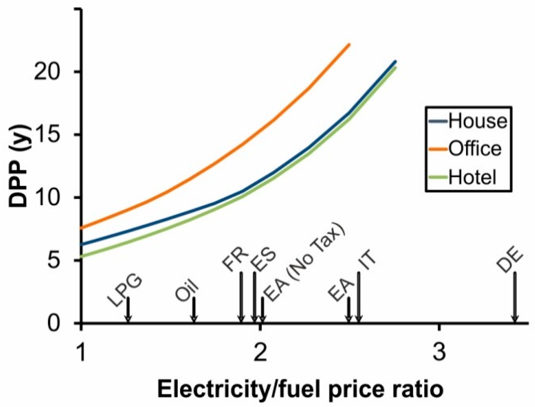
Figure 10 shows that the Discounted Payback Period grows exponentially with the ratio between electricity and the fossil fuel considered. In the present European price scenario, electricity is relatively expensive compared to natural gas, leaving little room for heat pump-driven revenues. This is partly due to the different taxation regimes, with a heavier taxation on electricity. If the GCHP replaced or prevented the installation of oil/LPG boilers (i.e., in areas not connected to methane pipelines), the electricity/fuel price ratio would be much lower, enabling profitable investments. The comparison between different countries shows that (geothermal) HPs installation in Germany is greatly penalized by the low gas price, while the low electricity price in France favors GCHP implementation.
3.3. Environmental Benefits
The environmental benefit of GCHP systems with respect to conventional systems was assessed, based on the simulation results, considering the non-renewable primary energy saved and the total CO2 emission avoided. Besides the efficiency of the GCHP system, the energy and environmental benefits mainly depend, respectively, on the non-renewable energy factor and the CO2 emission factor of the national grid. In Italy, the primary non-renewable energy factor of electrical energy is equal to 1.19 (ISPRA, 2017 [72]), while the emission factor for electricity (424 g CO2/kWh) and gas (240 g CO2/kWh) according to the Joint Research Centre (JRC) (2017, [73]).
In general, GCHPs reduce the primary energy consumption by 33–75% and CO2 emissions by 27–56% relative to conventional heating (gas boiler) and cooling (air chiller) systems. These two indicators are similar throughout the cases and mostly depend on the full load equivalent hours (FLEH) of the GCHP system operation, with lower results in cooling-dominated buildings, as the energy efficiency improvement given by GCHPs is higher in heating mode.
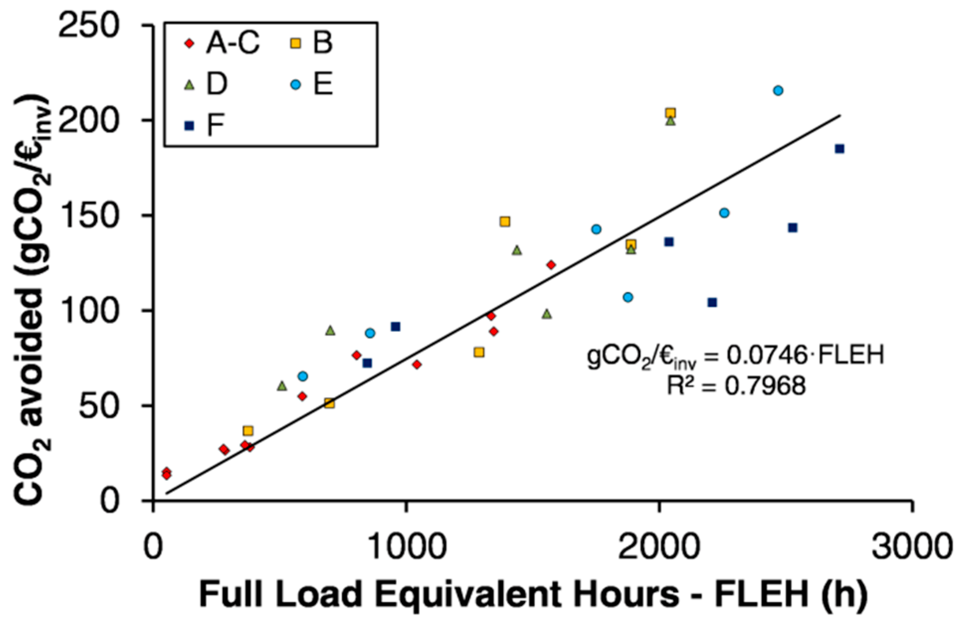
The effectiveness of investing in GCHPs to fight against climate changes can be expressed by the amount of avoided CO2 per year per Euro invested (Figure 11). With the aforementioned input data for the Italian case, this indicator ranges between 13 and 216 g CO2/€/year for the simulated cases, and it is proportional to the full load equivalent hours (FLEH) with a reduction 7.5 g CO2/€/year every 100 FLEH (). This indicator strongly depends on the CO2 emission factor of electricity, which varies depending on the source (if it is produced on site, e.g., with a PV plant) or, if it is taken from the grid, depending on the country. GCHPs global emissions are expected to reduce with time, along with the CO2 emission factor: for example, according to JRC, the Italian grid CO2 emission factor has fallen from 654 to 424 g CO2/kWh from 1990 to 2013 [73], and this reduction (−35%) is reflected on the CO2 emission factor of heat pumps, too.
The environmental performance of hybrid systems is slightly worse than GCHP systems, due to the consumption of natural gas to manage peak loads, but effectiveness of subsidies is increased due to the lower installation cost. Considering 90% and 70% of total energy demand met by HP, the primary energy and CO2 saved decrease as the share of the backup coverage increases; however, the CO2 avoided per Euro spent is 30% higher (in the 90% TEDM case) and 64% higher (in the 70% TEDM case) on average. This means that the GCHP-hybrid configuration is especially convenient to achieve the maximum results of incentives in terms of climate change mitigation.
The analysis on CO2 emissions performed for Italy was extended to the other 27 countries of the European Union, based on an emission assessment performed by the EU Joint Research Centre on the CO2 emission factor of the national electrical grids, with two methods (standard IPCC and LCA). The emission factors of electricity in EU-28 countries range from 15 g CO2/kWh of Sweden (38 g CO2/kWh with LCA) to 1977 g CO2/kWh of Estonia (2017 g CO2/kWh with LCA). Italy is close to the EU-28 average (respectively, 343 and 393 g CO2/kWh with the standard IPCC and the JRC LCA method). The full dataset is available in Table S16 of the Supplementary Materials, along with the calculation of the CO2 reduction achieved by a GCHP compared to a conventional HVAC system (gas boiler and air-source chiller), for which the minimum and the maximum reductions are shown. For highly carbon-intensive grids (i.e., higher than about 800 g CO2/kWh) such as in Bulgaria, Cyprus, Czech Republic, Estonia, Greece, Malta, and Poland, the use of GCHP can even lead to higher carbon dioxide emissions compared to a gas boiler. In the detail for each case study (Figure S6 of the Supplementary Materials), we observe that, for an average (Italy) and low (France) carbon emission factor, the highest reductions are achieved in the coldest climates (climate Zones D, E, F and, to a lesser extent, B, according to the classification by Tsikaloudaki et al. [33], since the main benefit is achieved by heating with the electrical heat pump, compared to gas. On the other hand, if electricity has a high emission factor (e.g., Poland), the GCHP in heating mode becomes more carbon-intensive than the gas boiler; in this case, a global CO2 emission reduction could be achieved only in the case of a cooling-dominated building, since both air-source chillers and GCHPs use electricity, and GCHPs are more efficient.
A further benefit of heat pumps (both ground and air-source ones) is related to air quality, which is a major issue especially for metropolitan areas. Heat pumps do not release pollutants in the air as they only consume electrical energy, usually generated elsewhere. The benefit compared to natural gas boilers on the air quality is rather limited, except for NOx [74], but it is much higher when compared to oil boilers (with high SOx emissions). The need to reduce the dependence on fossil fuel, however, makes it necessary to increase the share of renewable heat production. To date, the most used renewable heat source in Europe is still wood biomass in the form of wood logs, chips or pellets [75]. Their impact on particulate matter (PM10 and PM2.5), NOx and COV [76,77] has become hardly sustainable both in urban areas (e.g., Thessaloniki [78]) and in larger regions (e.g., the Po Plain in Italy [79]). Moreover, the supply chain of wood logs and pellets and hence their global environmental impact are critical, as demonstrated in various LCA studies [80,81]. If compared to biomass boilers, the electric energy production related to GCHP emits significantly less NOx (80–94%) and almost eliminates the particulate. The Fraunhofer Institute [82] studied the externality cost linked to NOx and PM10 emissions of biomasses, estimating externalities of 6 c€/kWh and 3 c€/kWh associated to wood log and pellet combustion, respectively. The internalisation of such costs would make biomasses more expensive of natural gas and, a fortiori, of heat pumps.
4. Conclusions
In this paper, the application of a ground-coupled heat pump (GCHP) in different buildings and climates was analyzed. The results highlight how climate, thermal insulation and building usage influence the required system capacity, annual energy consumption and, therefore, profitability and environmental benefits of the installation when compared to conventional systems.
A good thermal insulation (coping with present legislation) dramatically reduces both heating loads (50–70%) and heating demand (70–90%) compared to the typical insulation levels of the 1950s; cooling loads and needs in colder climate, are slightly increased, especially in Office buildings where internal heat gains are contained within the well-insulated envelope. Office buildings are also affected by long inactivity periods that imply high heating peak loads at the start-up of the HVAC system, in both heating and cooling modes (30–130% higher than other buildings), thus requiring a large-size plant which works at a few full-load equivalent hours per year (FLEH), compared to other building typologies. Conversely, in the Hotel case, the less variable schedule reduces the peak loads, thus increasing the heat pump (HP) yearly operational time. A substantial balance between building annual heating and cooling needs is found in temperate (B and D) climate zones for the highly-insulated cases. This is a desirable condition for the operation of reversible heat pumps and, in particular, for GHPs as it reduces the thermal imbalance of the ground and hence the required length of BHEs to be installed. Buildings in the coldest climates (Zones E and F), especially if poorly insulated, have the highest heating needs and utilize the HP extensively, a favorable condition to the use of GCHPs. On the other hand, buildings in warmer zones (A and C) are characterized by a low utilization factor in both heating and cooling modes, thus making it difficult to recover the investment on a GCHP. Domestic hot water consumption can represent a non-negligible part of the thermal needs (up to 80%) for well-insulated buildings in warm climates; however, the required peak load is very low and does not impact the system sizing process.
The building loads analysis proves that a large part of thermal energy consumptions can be covered with a fraction of the HP capacity (e.g., 60% of the peak load capacity meets 82–96% of the annual demand). This makes hybrid systems (HP and fossil-fuel boiler) an interesting solution to reduce the initial investment.
The economic analysis identifies the sustainability of a GCHP investment, revealing that public subsidies are essential to ensure the profitability, considering the energy prices in European countries. High energy consumption of buildings implies high revenues from the technology implementation; at the same time, reduced peak load determines a lower investment cost. Therefore, the most profitable building cases for GCHPs are the poorly insulated hotels placed in cold climates (payback times of 8.6–9.9 years). For the other cases analyzed, payback times are much longer and sometimes they exceed the system lifetime. Such a poor economic performance can be explained with the European average low price for natural gas and high price for electricity, reducing annual savings when HPs are compared to gas boilers. The economic return becomes easier in the case of substitution of an Oil/LPG heating system and in countries with lower electricity price such as France. The hybrid heat pump–gas boiler configuration is interesting as it reduces the system initial cost and thus improves the global economic results (20–40% payback period reduction).
Geothermal heat pumps reduce the primary energy consumption (33–75%) and the CO2 emissions (27–56%) with respect to conventional heating/cooling technologies (gas boiler and air-source chiller). Moreover, they have no emission on site, unlike fossil-fuel and biomass boilers, making HPs (both geothermal and aerothermal) a valuable solution for urban areas. The environmental effectiveness of private investment and public subsidies supporting GCHPs is quite high, with avoided emissions of 13–216 g CO2/year per euro spent; this performance can be enhanced by 30–81% with hybrid configurations, where the granted incentive is strongly reduced at the expense of a slightly smaller CO2 reduction.
This study provides a useful set of information for planning ground-coupled heat pumps in different contexts, identifying solutions to improve the economic viability of this technology, which remains the main barrier to its diffusion.
Supplementary Materials
The following are available online at https://www.mdpi.com/1996-1073/11/8/1941/s1: Table S1: Stratigraphy of the external wall in “good insulation” buildings; Table S2: Stratigraphy of the under-roof slab in the “good insulation” buildings; Table S3: Stratigraphy of the roof in the “good insulation” buildings; Table S4: Stratigraphy of the basement slab on cellar in the “good insulation” buildings; Table S5: Stratigraphy of the external wall in the “poor insulation” buildings; Table S6: Stratigraphy of the under-roof slab in the “poor insulation” buildings; Table S7: Stratigraphy of the roof in the “poor insulation” buildings; Table S8: Stratigraphy of the basement slab on cellar in the “poor insulation” buildings; Table S9: Occupancy levels (number of people) in the Hotel during different times at the first floor and upper floors. (WD, Working Days; WE, Weekend days); Table S10: Ventilation flow rates qve,k,mn expressed as number of air changes (h–1) in the Office building.; Table S11: Ventilation flow rates qve,k,mn expressed as number of air changes (h–1) in the Hotel building.; Table S12: Reference temperatures for design heating load in different climate zones; Table S13: Borehole heat exchangers and ground properties [7,8]; Table S14: Borehole total length for the different building and climates calculated with the ASHRAE method [9]; Table S15: Cost curve in Euro for different components related to specific capacities. A linear cost was supposed for the Borehole Heat Exchanger (BHE). (DHW: Domestic Hot Water, ACS: Air Conditioning System); Table S16: Electricity CO2 emission factors according to JRC (2017, [15]), calculated with two methods (standard and LCA), and the respective minimum and maximum CO2 emission reductions achieved in the 36 simulated cases. Figure S1: Specific heating demand for highly-insulated (A) and poorly-insulated (B) buildings, specific cooling demand for highly-insulated (C) and poorly-insulated (D) buildings; Figure S2: Full Load Equivalent Hours (FLEH) of heat pump operation for highly-insulated (A) and poorly-insulated (B) buildings in heating conditions, FLEH for highly-insulated (C) and poorly-insulated (D) buildings in cooling conditions.; Figure S3: Share of Domestic Hot Water (DHW) demand over the total energy demand for the different building cases in heating (A) and cooling (B) conditions.; Figure S4: Incidence of BHE costs on the total cost of a GCHP; Figure S5: Discounted Payback Period (DPP) compared with the electricity/fuel price ratio for the brand new highly-insulated buildings in climate Zone E (A), Net Present Value (NPV) compared with the electricity/fuel price ratio for the brand new highly-insulated buildings (B) and refurbished poorly-insulated building (C) in climate Zone E.; Figure S6: CO2 reduction achieved for the 36 simulated cases, using electricity from the grid with a low (France, 93 g CO2/kWh, in green), an average (Italy, 424 g CO2/kWh, in blue) and a high (Poland, 1090 g CO2/kWh, in red) CO2 emission factor. (Hou, House; Off, Office; Hot, Hotel; g, good insulation; p, poor insulation; A, B, C, D, E, and F, the climate zones according to Table 2 of the main text.
Author Contributions
Conceptualization: A.C., B.P., R.S. and M.R.; Formal analysis: M.R. and B.P.; Funding acquisition and project administration: R.S. and A.C.; Methodology: M.R., A.C., and B.P.; Supervision: R.S.; Visualization: M.R.; Writing—original draft: M.R., A.C., and B.P.; and Writing—review and editing: A.C. and R.S.
Funding
The study was performed in the framework of the project GRETA, which is co-financed by the European Regional Development Fund through the INTERREG Alpine Space program.
Acknowledgments
The authors gratefully acknowledge the contribution of Elena Dalla Vecchia, who assisted in the proofreading and language editing of the manuscript.
Conflicts of Interest
The authors declare to have no conflict of interest.
References
- IEA. World Energy Investment Outlook. 2014. Available online: www.iea.org/publications/freepublications/publication/WEIO2014.pdf (accessed on 27 November 2017).
- Polesello, V.; Johnson, K. Energy-Efficient Buildings for Low-Carbon Cities; ICCG Reflection; ICCG: Venice, Italy, 2016. [Google Scholar]
- Nejat, P.; Jomehzadeh, F.; Taheri, M.M.; Gohari, M.; Majid, M.Z. A global review of energy consumption, CO2 emissions and policy in the residential sector (with an overview of the top ten CO2 emitting countries). Renew. Sustain. Energy Rev. 2015, 43, 843–862. [Google Scholar] [CrossRef]
- Bayer, P.; Saner, D.; Bolay, S.; Rybach, L.; Blum, P. Greenhouse gas emission savings of ground source heat pump systems in europe: A review. Renew. Sustain. Energy Rev. 2012, 16, 1256–1267. [Google Scholar] [CrossRef]
- Heinonen, J.; Laine, J.; Pluuman, K.; Säynäjoki, E.-S.; Soukka, R.; Junnila, S. Planning for a low carbon future? Comparing heat pumps and cogeneration as the energy system options for a new residential area. Energies 2015, 8, 9137–9154. [Google Scholar] [CrossRef]
- Lund, J.W. Direct utilization of geothermal energy. Energies 2010, 3, 1443–1471. [Google Scholar] [CrossRef]
- Casasso, A.; Pestotnik, S.; Rajver, D.; Jež, J.; Prestor, J.; Sethi, R. Assessment and mapping of the closed-loop shallow geothermal potential in Cerkno (Slovenia). Energy Procedia 2017, 125, 335–344. [Google Scholar] [CrossRef]
- Casasso, A.; Sethi, R. Assessment and mapping of the shallow geothermal potential in the province of Cuneo (Piedmont, NW Italy). Renew. Energy 2017, 102, 306–315. [Google Scholar] [CrossRef]
- Yang, H.; Cui, P.; Fang, Z. Vertical-borehole ground-coupled heat pumps: A review of models and systems. Appl. Energy 2010, 87, 16–27. [Google Scholar] [CrossRef]
- Klein, S.A.; Beckman, W.A.; Mitchell, J.W.; Duffie, J.A.; Duffie, N.A.; Freeman, T.L.; Mitchell, J.C.; Braun, J.E.; Evans, B.L.; Kummer, J.P. Trnsys 16—User Manual; Solar Energy Laboratory, University of Wisconsin: Madison, WI, USA, 2004. [Google Scholar]
- Klein, S.A.; Beckman, W.A.; Mitchell, J.W.; Duffie, J.A.; Duffie, N.A.; Freeman, T.L.; Mitchell, J.C.; Braun, J.E.; Evans, B.L.; Kummer, J.P.; et al. Trnsys 16—Volume 3 Standard Component Library Overview; Solar Energy Laboratory, University of Wisconsin: Madison, WI, USA, 2005; p. 92. [Google Scholar]
- Zogou, O.; Stamatelos, A. Optimization of thermal performance of a building with ground source heat pump system. Energy Convers. Manag. 2007, 48, 2853–2863. [Google Scholar] [CrossRef]
- Fabrizio, E.; Ferrara, M.; Urone, G.; Corgnati, S.P.; Pronsati, S.; Filippi, M. Performance assessment of solar assisted ground source heat pump in a mountain site. Energy Procedia 2015, 78, 2286–2291. [Google Scholar] [CrossRef]
- Franco, A.; Fantozzi, F. Experimental analysis of a self consumption strategy for residential building: The integration of PV system and geothermal heat pump. Renew. Energy 2016, 86, 1075–1085. [Google Scholar] [CrossRef]
- Tagliabue, L.C.; Maistrello, M.; Del Pero, C. Solar heating and air-conditioning by gshp coupled to PV system for a cost effective high energy performance building. Energy Procedia 2012, 30, 683–692. [Google Scholar] [CrossRef]
- Thygesen, R.; Karlsson, B. An analysis on how proposed requirements for near zero energy buildings manages pv electricity in combination with two different types of heat pumps and its policy implications—A swedish example. Energy Policy 2017, 101, 10–19. [Google Scholar] [CrossRef]
- Ruiz-Calvo, F.; Montagud, C.; Cazorla-Marín, A.; Corberán, J.M. Development and experimental validation of a TRNSYS dynamic tool for design and energy optimization of ground source heat pump systems. Energies 2017, 10, 1510. [Google Scholar] [CrossRef]
- De Rosa, M.; Ruiz-Calvo, F.; Corberán, J.M.; Montagud, C.; Tagliafico, L.A. A novel trnsys type for short-term borehole heat exchanger simulation: B2G model. Energy Convers. Manag. 2015, 100, 347–357. [Google Scholar] [CrossRef]
- Ruiz-Calvo, F.; De Rosa, M.; Monzó, P.; Montagud, C.; Corberán, J.M. Coupling short-term (B2G model) and long-term (g-function) models for ground source heat exchanger simulation in trnsys. Application in a real installation. Appl. Therm. Eng. 2016, 102, 720–732. [Google Scholar] [CrossRef]
- Emmi, G.; Zarrella, A.; De Carli, M.; Galgaro, A. An analysis of solar assisted ground source heat pumps in cold climates. Energy Convers. Manag. 2015, 106, 660–675. [Google Scholar] [CrossRef]
- Montagud, C.; Corberán, J.M.; Ruiz-Calvo, F. Experimental and modeling analysis of a ground source heat pump system. Appl. Energy 2013, 109, 328–336. [Google Scholar] [CrossRef] [Green Version]
- Han, C.; Yu, X. Performance of a residential ground source heat pump system in sedimentary rock formation. Appl. Energy 2016, 164, 89–98. [Google Scholar] [CrossRef] [Green Version]
- Safa, A.A.; Fung, A.S.; Kumar, R. Heating and cooling performance characterisation of ground source heat pump system by testing and TRNSYS simulation. Renew. Energy 2015, 83, 565–575. [Google Scholar] [CrossRef]
- Zhao, Z.; Shen, R.; Feng, W.; Zhang, Y.; Zhang, Y. Soil thermal balance analysis for a ground source heat pump system in a hot-summer and cold-winter region. Energies 2018, 11, 1206. [Google Scholar] [CrossRef]
- Jung, Y.-J.; Kim, H.-J.; Choi, B.-E.; Jo, J.-H.; Cho, Y.-H. A study on the efficiency improvement of multi-geothermal heat pump systems in Korea using coefficient of performance. Energies 2016, 9, 356. [Google Scholar] [CrossRef]
- Lu, Q.; Narsilio, G.A.; Aditya, G.R.; Johnston, I.W. Economic analysis of vertical ground source heat pump systems in melbourne. Energy 2017, 125, 107–117. [Google Scholar] [CrossRef]
- Morrone, B.; Coppola, G.; Raucci, V. Energy and economic savings using geothermal heat pumps in different climates. Energy Convers. Manag. 2014, 88, 189–198. [Google Scholar] [CrossRef]
- Chang, Y.; Gu, Y.; Zhang, L.; Wu, C.; Liang, L. Energy and environmental implications of using geothermal heat pumps in buildings: An example from North China. J. Clean. Prod. 2017, 167, 484–492. [Google Scholar] [CrossRef]
- Ciulla, G.; Lo Brano, V.; D’Amico, A. Modelling relationship among energy demand, climate and office building features: A cluster analysis at european level. Appl. Energy 2016, 183, 1021–1034. [Google Scholar] [CrossRef]
- Junghans, L. Evaluation of the economic and environmental feasibility of heat pump systems in residential buildings, with varying qualities of the building envelope. Renew. Energy 2015, 76, 699–705. [Google Scholar] [CrossRef]
- Alavy, M.; Nguyen, H.V.; Leong, W.H.; Dworkin, S.B. A methodology and computerized approach for optimizing hybrid ground source heat pump system design. Renew. Energy 2013, 57, 404–412. [Google Scholar] [CrossRef]
- Nguyen, H.V.; Law, Y.L.E.; Alavy, M.; Walsh, P.R.; Leong, W.H.; Dworkin, S.B. An analysis of the factors affecting hybrid ground-source heat pump installation potential in North America. Appl. Energy 2014, 125, 28–38. [Google Scholar] [CrossRef]
- Tsikaloudaki, K.; Laskos, K.; Bikas, D. On the Establishment of Climatic Zones in Europe with Regard to the Energy Performance of Buildings. Energies 2011, 5, 32–44. [Google Scholar] [CrossRef] [Green Version]
- Italian Ministry of Economic Development. Supplemento Ordinario n.39 alla Gazzetta Ufficiale—Serie Generale—n.162; Repubblica Italiana: Rome, Italy, 2015; pp. 1–41.
- Ballarini, I.; Corgnati, S.P.; Corrado, V. Use of reference buildings to assess the energy saving potentials of the residential building stock: The experience of TABULA project. Energy Policy 2014, 68, 273–284. [Google Scholar] [CrossRef]
- Meteonorm. Meteonorm—Irradiation Data for Every Place on Earth. Available online: www.meteonorm.com/ (accessed on 31 January 2018).
- Klein, S.A.; Beckman, W.A.; Mitchell, J.W.; Duffie, J.A.; Duffie, N.A.; Freeman, T.L.; Mitchell, J.C.; Braun, J.E.; Evans, B.L.; Kummer, J.P.; et al. Trnsys 16—Volume 6 Multizone Building Modeling with Type 56 and Trnbuild; Solar Energy Laboratory, University of Wisconsin: Madison, WI, USA, 2004; p. 199. [Google Scholar]
- Aprile, M. Caratterizzazione Energetica del Settore Alberghiero in Italia (Energy Characterisation of the Hotel Sector in Italy). Available online: progettoegadi.enea.it/it/RSE162.pdf (accessed on 3 May 2017).
- Klein, S.A.; Beckman, W.A.; Mitchell, J.W.; Duffie, J.A.; Duffie, N.A.; Freeman, T.L.; Mitchell, J.C.; Braun, J.E.; Evans, B.L.; Kummer, J.P.; et al. Trnsys 16—Volume 5 Mathematical Reference; Solar Energy Laboratory, University of Wisconsin: Madison, WI, USA, 2006; p. 434. [Google Scholar]
- TESS (Thermal Energy System Specialists). Tess Library Documentation; TESS: Madison, WI, USA, 2004. [Google Scholar]
- UNI/TS. Uni ts 11300-1: Prestazioni Energetiche Degli Edifici, Parte 1. Available online: http://www.dabove.com/index.php?page=la-norma-uni-ts-11300-1 (accessed on 14 June 2018).
- Rabl, A.; Norford, L. Peak load reduction by preconditioning buildings at night. Int. J. Energy Res. 1991, 15, 781–798. [Google Scholar] [CrossRef]
- Dimplex. Manuale di Progettazione. Riscaldare e Raffreddare con Pompe di Calore (Design Manual. Heating and Cooling with Heat Pumps). Available online: goo.gl/LehE2v (accessed on 27 April 2017).
- Ochsner, K. Geothermal Heat Pumps: A Guide for Planning and Installing; Routledge: London, UK, 2012. [Google Scholar]
- ASHRAE. Handbook-Fundamentals; ASHRAE: Atlanta, GA, USA, 2013. [Google Scholar]
- UNI/TS. Uni ts 11300-2: Prestazioni Energetiche Degli Edifici, Parte 2. Available online: http://www.dabove.com/index.php?page=la-norma-uni-ts-11300-2 (accessed on 14 June 2018).
- Jordan, U.; Vajen, K. Realistic Domestic Hot-Water Profiles in Different Time Scales. Available online: goo.gl/7Nkzzq (accessed on 6 May 2017).
- Hellström, G. Duct Ground Heat Storage Model, Manual for Computer Code; Department of Mathematical Physics, University of Lund: Lund, Sweden, 1989. [Google Scholar]
- Philippe, M.; Michel Bernier, P.; Marchio, D. Sizing calculation spreadsheet: Vertical geothermal borefields. Ashrae J. 2010, 52, 20. [Google Scholar]
- Kavanaugh, S.P.; Rafferty, K. Ground-Source Heat Pumps: Design of Geothermal Systems for Commercial and Institutional Buildings; ASHRAE: Atlanta, GA, USA, 1997. [Google Scholar]
- Belussi, L.; Danza, L. Method for the prediction of malfunctions of buildings through real energy consumption analysis: Holistic and multidisciplinary approach of energy signature. Energy Build. 2012, 55, 715–720. [Google Scholar] [CrossRef]
- Ni, L.; Song, W.; Zeng, F.; Yao, Y. Energy Saving and Economic Analyses of Design Heating Load Ratio of Ground Source Heat Pump with Gas Boiler as Auxiliary Heat Source. In Proceedings of the IEEE 2011 International Conference on Electric Technology and Civil Engineering (ICETCE), Jiujiang, China, 22–24 April 2011; pp. 1197–1200. [Google Scholar]
- Bierman, H., Jr.; Smidt, S. The Capital Budgeting Decision: Economic Analysis of Investment Projects; Routledge: London, UK, 2012. [Google Scholar]
- EIA. Updated Buildings Sector Appliance and Equipment Costs and Efficiencies. Available online: www.eia.gov/analysis/studies/buildings/equipcosts/pdf/full.pdf (accessed on 28 June 2017).
- IEA. Renewables for Heating and Cooling. Available online: www.iea.org/publications/freepublications/publication/Renewable_Heating_Cooling_Final_WEB.pdf (accessed on 27 June 2017).
- European Central Bank. Harmonised Long-Term Interest Rates. Available online: www.ecb.europa.eu/stats/shared/download/stats/download/irs/irs/irs.pdf (accessed on 17 July 2017).
- Ochsner. Price List 2012. Available online: wagnersolar.hu/dokumentumok/OCHSNER_Arlista2012-2.pdf (accessed on 27 April 2017).
- Vaillant. Listino Prezzi Settembre 2016 (Price List September 2016). Available online: goo.gl/eYAcFC (accessed on 30 June 2017).
- Viessmann. Price List. Available online: www.viessmann.de (accessed on 30 June 2017).
- Bosch. Listino Prezzi 2016 (Price List 2016). Available online: www.junkers.it/privati/documentazione/cataloghi_e_listini/cataloghi_e_listini (accessed on 30 June 2017).
- Hoval Hoval website. Available online: www.hoval.it/ (accessed on 27 April 2017).
- BRGM. Qualiforage. Engagement of Borehole Heat Exchanger Drilling Enterprises. Available online: infoterre.brgm.fr/rapports/RP-63015-FR.pdf (accessed on 2 July 2017).
- Agenzia Delle Entrate. Guida Agevolazioni Risparmio Energetico 2017 (Guide to Incentives for Energy Saving). Available online: goo.gl/boZuRg (accessed on 5 July 2017).
- European Commission. Vat Rates Applied in the Member States of the European Union. Situation at 1st January 2018. Available online: https://ec.europa.eu/taxation_customs/sites/taxation/files/resources/documents/taxation/vat/how_vat_works/rates/vat_rates_en.pdf (accessed on 8 July 2018).
- Eurostat. Eurostat Website. Available online: ec.europa.eu/eurostat (accessed on 8 July 2017).
- European Commission. Consumer Prices of Petroleum Products. Available online: ec.europa.eu/energy/en/data-analysis/weekly-oil-bulletin (accessed on 18 October 2017).
- Winkler, J.; Booten, C.; Christensen, D.; Tomerlin, J. Laboratory Performance Testing of Residential Window Air Conditioners. Available online: goo.gl/L6ykA8 (accessed on 3 August 2017).
- Buckley, C.; Pasquali, R.; Lee, M.; Dooley, J.; Williams, T. Ground Source Heat and Shallow Geothermal Energy Homeowner Manual. Available online: goo.gl/7L1tcE (accessed on 6 September 2017).
- Newnan, D.G.; Eschenbach, T.; Lavelle, J.P. Engineering Economic Analysis; Oxford University Press: Oxford, UK, 2004; Volume 2. [Google Scholar]
- Chinese, D.; Nardin, G.; Saro, O. Multi-criteria analysis for the selection of space heating systems in an industrial building. Energy 2011, 36, 556–565. [Google Scholar] [CrossRef]
- IEA. Monthly Oil Price Statistics. Available online: www.iea.org/statistics/monthlystatistics/monthlyoilprices/ (accessed on 18 October 2017).
- ISPRA. Fattori di Emissione Atmosferica di CO2 e Altri Gas a Effetto Serra nel Settore Elettrico (CO2 Emission Factors of the Electric Sector). Available online: www.isprambiente.gov.it/files2017/pubblicazioni/rapporto/R_257_17.pdf (accessed on 19 November 2017).
- Koffi, B.; Cerutti, A.; Duerr, M.; Iancu, A.; Kona, A.; Janssens-Maenhout, G. Com Default Emission Factors for the Member States of the European Union. Available online: data.europa.eu/89h/jrc-com-ef-comw-ef-2017 (accessed on 13 July 2018).
- ARPA Lombardia; Regione Lombardia; Regione Piemonte; Regione Emilia Romagna; Regione Veneto; Giulia, R.F.-V.; Regione Puglia; Provincia di Trento; Provincia di Bolzano. Inemar—Inventario Emssioni Aria (Inventory of Emissions of Air Pollutants). Available online: http://www.inemar.eu/ (accessed on 10 December 2017).
- INNOVHUB. Comparative Study on the Emissions of Gas, LPG, Oil and Pellet Boilers. Available online: goo.gl/GmhhKn (accessed on 15 December 2017).
- Shen, G.; Tao, S.; Wei, S.; Zhang, Y.; Wang, R.; Wang, B.; Li, W.; Shen, H.; Huang, Y.; Chen, Y.; et al. Reductions in emissions of carbonaceous particulate matter and polycyclic aromatic hydrocarbons from combustion of biomass pellets in comparison with raw fuel burning. Environ. Sci. Technol. 2012, 46, 6409–6416. [Google Scholar] [CrossRef] [PubMed]
- Ozgen, S.; Caserini, S.; Galante, S.; Giugliano, M.; Angelino, E.; Marongiu, A.; Hugony, F.; Migliavacca, G.; Morreale, C. Emission factors from small scale appliances burning wood and pellets. Atmos. Environ. 2014, 94, 144–153. [Google Scholar] [CrossRef]
- Sarigiannis, D.A.; Karakitsios, S.P.; Kermenidou, M.V. Health impact and monetary cost of exposure to particulate matter emitted from biomass burning in large cities. Sci. Total Environ. 2015, 524–525, 319–330. [Google Scholar] [CrossRef] [PubMed]
- Pietrogrande, M.C.; Bacco, D.; Ferrari, S.; Kaipainen, J.; Ricciardelli, I.; Riekkola, M.L.; Trentini, A.; Visentin, M. Characterization of atmospheric aerosols in the po valley during the supersito campaigns—Part 3: Contribution of wood combustion to wintertime atmospheric aerosols in Emilia Romagna region (Northern Italy). Atmos. Environ. 2015, 122, 291–305. [Google Scholar] [CrossRef]
- McKechnie, J.; Colombo, S.; Chen, J.; Mabee, W.; MacLean, H.L. Forest bioenergy or forest carbon? Assessing trade-offs in greenhouse gas mitigation with wood-based fuels. Environ. Sci. Technol. 2010, 45, 789–795. [Google Scholar] [CrossRef] [PubMed]
- Ter-Mikaelian, M.T.; Colombo, S.J.; Chen, J. The burning question: Does forest bioenergy reduce carbon emissions? A review of common misconceptions about forest carbon accounting. J. For. 2015, 113, 57–68. [Google Scholar] [CrossRef]
- Fraunhofer Institute. Ermittlung Vermiedener Umweltschäden—Hintergrundpapier zur Methodik—Im: “Rahmen des Projekts Wirkungen des Ausbaus Erneuerbarer Energien” (Determination of Avoided Environmental Damage—Background Paper on Methodology. In Impact of the Expansion of Renewable Energies; Fraunhofer Institute: Munich, Germany, 2012; Available online: publica.fraunhofer.de/eprints/urn_nbn_de_0011-n-2363162.pdf (accessed on 5 January 2018).
Figure 1.
Climatic classification of major European cities according to Heating/Cooling Degree Days (HDD/CDD) criteria reported in Table 4.
Figure 1.
Climatic classification of major European cities according to Heating/Cooling Degree Days (HDD/CDD) criteria reported in Table 4.

Figure 2.
Building-HVAC integrated model on TRNSYS Studio. (AHU, Air Handling Unit; DHW, Domestic Hot Water; HP, Heat Pump; BHE, Borehole Heat Exchangers).
Figure 2.
Building-HVAC integrated model on TRNSYS Studio. (AHU, Air Handling Unit; DHW, Domestic Hot Water; HP, Heat Pump; BHE, Borehole Heat Exchangers).

Figure 3.
Heating and cooling COP map for a heat pump with a peak heating power of 10.5 kW.

Figure 4.
Heating peak loads with good insulation (A) and poor insulation (B) cooling peak loads with good insulation (C) and poor insulation (D), in different climate zones identified in Table 2.
Figure 4.
Heating peak loads with good insulation (A) and poor insulation (B) cooling peak loads with good insulation (C) and poor insulation (D), in different climate zones identified in Table 2.

Figure 5.
Heating signature for well-insulated (A) and poorly-insulated (B) buildings; cooling signature for the well-insulated (C) and poorly-insulated (D) buildings.
Figure 5.
Heating signature for well-insulated (A) and poorly-insulated (B) buildings; cooling signature for the well-insulated (C) and poorly-insulated (D) buildings.

Figure 6.
Load factor vs. TEDM (Total Energy Demand Met by the heat pump) in heating season for the simulations performed.
Figure 6.
Load factor vs. TEDM (Total Energy Demand Met by the heat pump) in heating season for the simulations performed.

Figure 7.
Heating and cooling SPF (Seasonal Performance Factor) vs. annual mean air temperature.

Figure 8.
Discount Payback Period (DPP, [54]) for the subsidized GCHP system installation in poorly-insulated building refurbishing cases in the different climate zones (Table 2).

Figure 9.
Estimated vs. simulated load curves for the high-insulated House in climate Zone E.

Figure 10.
Discounted Payback Period (DPP, [54]) of subsidized GCHP system in low-insulated buildings in Zone E vs. different electricity/fuel price ratio.
Figure 10.
Discounted Payback Period (DPP, [54]) of subsidized GCHP system in low-insulated buildings in Zone E vs. different electricity/fuel price ratio.

Figure 11.
GHG reduction effectiveness of GCHPs in Italy, expressed as CO2 avoided emissions per euro spent, plotted against the system Full Load Equivalent Hours (FLEH) of operation. The dots, representing every GCHP simulated, are provided with a color code which identifies the specific climate zone (A–F).


Table 1.
Buildings features. (S/V ratio = external Surface area to gross Volume ratio).
| Building | Floor Area (m2) | External Surface (m2) | Gross Volume (m3) | S/V Ratio (m−1) |
|---|---|---|---|---|
| House | 221 | 556 | 855 | 0.65 |
| Office | 381 | 953 | 1832 | 0.52 |
| Hotel | 2840 | 4374 | 15,620 | 0.28 |
Table 2.
Thermal transmittance value of opaque elements of the building envelope for “Good insulation” and “Poor insulation” buildings.
Table 2.
Thermal transmittance value of opaque elements of the building envelope for “Good insulation” and “Poor insulation” buildings.
| Element | U-Value (W/(m2 K)) “Good Insulation” | U-Value (W/(m2 K)) “Poor Insulation” |
|---|---|---|
| External wall | 0.28 | 1.60 |
| Under-roof slab | 0.51 | 1.76 |
| Roof | 0.24 | 2.38 |
| Floor | 0.15 | 0.75 |
Table 3.
Thermal properties of windows for “Good insulation” and “Poor insulation” buildings.
| Property | Good Insulation | Poor Insulation |
|---|---|---|
| Window type | Double 4/15/4 | Single 4 |
| U-value (W/m2 K) | 1.430 | 5.680 |
| g-value | 0.605 | 0.855 |
| Transmittance | 0.521 | 0.830 |
| Reflectance | 0.355 | 0.075 |
Table 4.
Studied cities for each European climate zone defined by Tsikaloudaki et al. [33] (HDD, Heating Degree Days; CDD, Cooling Degree Days; values calculated with Meteonorm data [36]).
| Climate Zone | HDD Criterion | CDD Criterion | City | Average Annual Temperature | HDD | CDD |
|---|---|---|---|---|---|---|
| A | <1500 | ≥500 | Seville, Spain | 18.18 °C | 920 | 986 |
| B | 1500–3000 | ≥500 | Bologna, Italy | 13.98 °C | 2115 | 649 |
| C | <1500 | <500 | Lisbon, Portugal | 16.81 °C | 914 | 480 |
| D | 1500–3000 | <500 | Belgrade, Serbia | 11.26 °C | 2743 | 239 |
| E | 3000–3750 | <500 | Berlin, Germany | 9.42 °C | 3172 | 41 |
| F | ≥3750 | <500 | Stockholm, Sweden | 5.31 °C | 4632 | 0 |
Table 5.
Heating and cooling schedules for different buildings. (Monday has a different schedule for the Office case to extend the heat up period and reduce the peak load after the weekend. WD, Other Working Days; WE, Weekend days.)
Table 5.
Heating and cooling schedules for different buildings. (Monday has a different schedule for the Office case to extend the heat up period and reduce the peak load after the weekend. WD, Other Working Days; WE, Weekend days.)
| Mode | Building | Monday | WD | WE |
|---|---|---|---|---|
| Heating | House | 6:00–8:00 a.m. and 4:00–10:00 p.m. | 6:00 –8:00 a.m. and 4:00–10:00 p.m. | 8:00 a.m.–10:00 p.m. |
| Office | 4:00 a.m.–6:00 p.m. | 6:00 a.m.–6:00 p.m. | Always off | |
| Hotel | Always on | Always on | Always on | |
| Cooling | House | 4:00–10:00 p.m. | 4:00–10:00 p.m. | 8:00 a.m.–10:00 p.m. |
| Office | 7:00 a.m.–6:00 p.m. | 8:00 a.m.–6:00 p.m. | Always off | |
| Hotel | Always on | Always on | Always on |
Table 6.
Economic feasibility of GCHP system installation in different buildings at actual energy prices. (-, not feasible investments; !, investments with low internal rate of return; +, feasible investments).
Table 6.
Economic feasibility of GCHP system installation in different buildings at actual energy prices. (-, not feasible investments; !, investments with low internal rate of return; +, feasible investments).
| Installation Type | Climate Zone | Subsidies | No Subsidies | ||||
|---|---|---|---|---|---|---|---|
| House | Office | Hotel | House | Office | Hotel | ||
| New installation | A | ! | - | ! | - | - | - |
| B | + | ! | ! | - | - | - | |
| C | ! | - | - | - | - | - | |
| D | + | ↑ | ↑ | - | - | - | |
| E | + | ↑ | ↑ | - | - | - | |
| F | + | ↑ | ↑ | - | - | - | |
| Substitution | A | ! | ! | + | - | - | - |
| B | + | + | + | ! | ! | + | |
| C | + | ! | + | - | - | ! | |
| D | + | + | + | - | - | + | |
| E | + | + | + | ! | - | + | |
| F | + | + | + | - | - | + | |
Table 7.
Average simulated Total Energy Demand Met (TEDM) by the heat pump in comparison with the TEDM estimated from the building load curves.
Table 7.
Average simulated Total Energy Demand Met (TEDM) by the heat pump in comparison with the TEDM estimated from the building load curves.
| Building | House | Office | Hotel |
|---|---|---|---|
| 90% estimated TEDM | 87% | 97% | 98% |
| 70% estimated TEDM | 68% | 88% | 91% |
Table 8.
Electricity/fuel price ratio for different fuels and countries. (EA, Euro Area electricity/gas price ratio; Oil, heating oil as fuel; LPG, heating LPG as fuel).
Table 8.
Electricity/fuel price ratio for different fuels and countries. (EA, Euro Area electricity/gas price ratio; Oil, heating oil as fuel; LPG, heating LPG as fuel).
| Present EA | EA (No Taxes) | Oil (IT) | LPG (IT) | IT | DE | ES | FR |
|---|---|---|---|---|---|---|---|
| 2.53 | 2.04 | 1.64 | 1.27 | 2.59 | 3.48 | 1.99 | 1.91 |
© 2018 by the authors. Licensee MDPI, Basel, Switzerland. This article is an open access article distributed under the terms and conditions of the Creative Commons Attribution (CC BY) license (http://creativecommons.org/licenses/by/4.0/).
Share and Cite
MDPI and ACS Style
Rivoire, M.; Casasso, A.; Piga, B.; Sethi, R. Assessment of Energetic, Economic and Environmental Performance of Ground-Coupled Heat Pumps. Energies 2018, 11, 1941. https://doi.org/10.3390/en11081941
AMA Style
Rivoire M, Casasso A, Piga B, Sethi R. Assessment of Energetic, Economic and Environmental Performance of Ground-Coupled Heat Pumps. Energies. 2018; 11(8):1941. https://doi.org/10.3390/en11081941
Chicago/Turabian StyleRivoire, Matteo, Alessandro Casasso, Bruno Piga, and Rajandrea Sethi. 2018. "Assessment of Energetic, Economic and Environmental Performance of Ground-Coupled Heat Pumps" Energies 11, no. 8: 1941. https://doi.org/10.3390/en11081941
Note that from the first issue of 2016, this journal uses article numbers instead of page numbers. See further details here.