Network Features of the EU Carbon Trade System: An Evolutionary Perspective

1
Institute of Science and Development, Chinese Academy of Sciences, Beijing 100190, China
2
School of Humanities and Economic Management, China University of Geosciences, Beijing 100083, China
3
School of Public Policy and Management, University of Chinese Academy of Sciences, Beijing 100049, China
*
Author to whom correspondence should be addressed.
Energies 2018, 11(6), 1501; https://doi.org/10.3390/en11061501
Submission received: 28 April 2018
/
Revised: 2 June 2018
/
Accepted: 5 June 2018
/
Published: 8 June 2018
(This article belongs to the Special Issue Lessons from the Evaluation of Existing Emission Trading Schemes)
Abstract
:In this paper, a network model is constructed using real trading data from the EU carbon market. Metric indicators are then introduced to measure the network, and the economic meanings of the indicators are discussed. By integrating time windows with the network model, three types of network features are examined: growth features, structural features, and scale-free features. The growth pattern of the carbon trading network is then analyzed. As the market grow, the geodesic distances become shorter and the clustering coefficients become larger. The trends of these two indicators suggest that the market is evolving towards efficiency; however, their tiny changes are insufficient to have significant impact. By modeling the heterogeneity of the carbon trading network, we find that the trading relationships between firms obey a broken power law model, which consists of two power law models. The broken power law model can be approximately defined as a traditional power law but with a longer tail in distribution. Furthermore, we find that the model is valid for most of the time of both phases, the model only invalid when the market approaches a high growth rate.
1. Introduction
Emission trading schemes (ETS) are one of the preferred tools for combating climate change. Following the cap-and-trade principle, they are a cost-effective method for reducing greenhouse gas (GHG) emissions. Several countries and regions have launched emissions trading schemes, including the European Union, Japan, South Korea, and China. The biggest one by far is the European ETS; known as the European Union Emission Trading Scheme (EU ETS), which includes more than 11,000 heavily emitting installations from 31 European countries, representing more than 45% of Europe’s overall GHG emissions. In the EU scheme, the right to emit CO2 is represented by carbon allowances, primarily the European Union Allowances (EUA).
In the first two phases of the EU ETS, EUAs were freely allocated to emitters according to their emission history. Thereafter, emitters have been obliged to cover their annual CO2 emissions with equivalent allowances through a process called surrender. A deficiency of allowances compared to actual emissions brings emitters a penalty; emitters therefore trade and buy allowances from each other, giving emitters with spare allowances an incentive to sell their allowances [1,2].
After 10 years of development, the EU ETS has become the largest carbon market in the world. Generally, participants in the EU carbon markets can be categorized as belonging to one of three types: governments, emitters, or financial institutions. First, the purpose of the government entities is to regulate the allocation and surrender of allowances. Second, the emitters trade carbon allowances based on market supply and demand. Third, the financial institutions are not themselves subject to emission regulations, but act as intermediaries in the carbon trade [3]. Thus, the governments are the market regulators, while the emitters and financial institutions—real EU-based firms—are the market players.
In the EUA market, the emitters can trade allowances through three types of transaction: bilateral transactions, Over-the-counter (OTC) transactions, and transactions on organized exchanges. In bilateral transactions, two emitters can directly trades allowances with each other without using intermediaries. The price on the bilateral transactions are not disclosed to public. OTC transactions are executed by intermediaries for facilitating trading between various emitters. The intermediaries in the OTC market help emitters to find a seller or buyer, and negotiate the deal. The price and volume of the OTC transactions are not available to public. The organized exchanges on EUA trading emerged in mid-2005, such as ECX, EEX, BlueNext and so on. Traders in the organized exchanges trade EUA anonymously through electronic platforms, the exchanges release the settlement price and total volume timely on their platform.
The literature on carbon markets mostly focuses on market performance, such as price dynamics [4,5,6], market efficiency [7,8], trading behaviors [9,10], and firm performance [11,12]. However, the market structure and its evolution are seldom mentioned [13]. Over the past decades, thousands of firms have participated in the Emission trading schemes and ten thousands of trading relationships set up between firms in the EU carbon market, which form a complex trading network. Thus, the emission trading market is a complex and nonlinear system. In order to understand the emission trading behaviors in the market, we should detect the complex emission trading relationships between thousands of firms clearly. Complex network theory provides a particular approach for studying the structure of the emission trading market. The advantage of the complex network theory is to understand the essential nature of the system operation by abstracting the elements and the relationships between elements as complex network. Because the core idea of the complex network theory is that the network structure determines the system function [14]. Recently, complex network theory has become increasingly popular in commodity market and emission research [15,16,17,18] because it reveals market structure through the relationships between traders. Using firm-level emissions trading data, the carbon market can be modeled as a network, whose nodes are firms and whose edges are the trading relationships between companies.
With the growth of the emission trading market, the market structure become more and more complex. There may be different structures of the emission trading market in different periods. It means that the emission trading behaviors between firms may show different characteristics with the development of the emission trading market. Thus, in order to understand the evolutionary characteristics of the emission trading networks, we divide the development history of the EU carbon market into a series of periods by time windows. Then we analyzing the evolutionary characteristics of the carbon trade network by metric complex network analysis indicators. This paper provides a novel perspective on the structure of the EU carbon market.
2. Data
The carbon trading data used in this research comes from the European Union Transaction Log (EUTL), which is a database that records each transfer of allowances in the EU ETS. The data are published with a 3-year delay, so the latest data available are from April 2014. The data used for this paper span from January 2005 to April 2014 and contain more than 800,000 allowance transfers. In previous work, we analyzed the data structure [19] and tested its completeness [20], and we found that the EUTL data presents a closed system of allowance circulation, in which a specific quantity of allowances are transferred between finite accounts. The allowance transfers can be divided into two types: regulated transfers and trading. The former is driven by the policies and regulations of the EU ETS, while the latter is driven by market mechanisms.
The EUTL data is presented at the account level; however, the carbon market is identified at the level of firms. Therefore, we identified all of the firms in the EUTL data and transformed the account-level trading data into firm-level data by associating each account with a firm. Firms can trade allowances using two types of account: operator holding accounts (OHA) and person holding accounts (PHA). Each OHA is associated with a unique CO2 emitting installation, so if a single firm owns multiple emitting installations, they will have multiple OHAs. The allocation and surrender of allowances must be executed through OHAs; PHAs, in contrast, can only trade allowances. In this paper, emitters are defined as companies which hold at least one OHA, while all other firms are defined as financial institutions.
The data can be easily divided in to two phases according to the types of emissions unit and allowances that were traded in the market. In the Phase I data, which span from January 2005 to April 2008, only a specific type of allowance was traded, called non-Kyoto allowances. However, in Phase II, which spanned from January 2008 to April 2013, the trades included EUAs, certified emissions reductions, emission reduction units, and aviation allowances. The EU ETS data also contains some trading data for Phase III, but the data is insufficient for analysis.
Table 1 gives an overview of the data. In Phase I, there were 8214 OHAs and 782 PHAs, which belonged to 4711 emitters and 15 financial institutions. The number of trades between those accounts was 48,931. When accounts were attached to firms, the data showed that there were 41,490 trades between different firms, while the other trades took place within firms. In Phase II, the number of firms is 6681, of which 6349 were emitters while 332 were financial institutions.
3. Methods
3.1. Construction of the Carbon Trade Network
In this paper, we assume that once two firms have traded allowances in the EU carbon market, a long-term relationship will be built between them. Moreover, we assume that firms in a relationship will receive information about each other, making them more trustful of each other for future trades. In the EU carbon markets, the trading relationships thus increase the connectivity of the market and enable allowances to circulate effectively among firms.
Based on the firm-level carbon trading data, an undirected and unweighted network can be built to model the trading relationships between firms in the EU ETS. The nodes represent the firms, and its edges are the binary trading relationships between firms. is the number of nodes and is the number of edges. ( describes the size of a set). The edges are undirected because the trading relationship is mutual to both firms.
3.2. Network Metric Indicators
To observe the structural features of the carbon trading networks, we introduce three metric indicators with specific meanings in economics, namely network density, average geodesic distances, and average clustering coefficients. The definitions and economic meanings of these indicators are presented as follows:
1. Network density
Network density describes the portion of the potential connections in a network that are actual connections. Supposing there are n nodes and m edges in a network G, the maximum number of edges that a n-nodes network can reach is n(n − 1), so the density of the network is:
2. Average geodesic distance
A geodesic path is the shortest path between two nodes. Formally, given a path between two nodes, the length of this path is given by . Let for the set of all paths between nodes and . Therefore, the geodesic path is defined by:
The identification of the geodesic paths is based on the Dijkstra algorithm. The average geodesic distance of a network is given by:
In most real-world networks, a short average path length facilitates the quick transfer of information and materials. In this paper, the efficiency of carbon trading can be judged by studying its average geodesic distance. A lower average geodesic distance suggests that firms are easily able to find appropriate buyers or sellers, therefore indicating that the market is more efficient.
3. Average clustering coefficient
In the carbon trading network, although a firm A and a firm B may both have trading relationships with a firm C, firms A and B may or may not have direct trading relationships with each other. For a firm with many trading partners, if its partners do not build direct trading relationships with each other, then transfers of information and allowances are highly dependent on the willingness of the centered firm to manage the flow of data and trading. It can be said that the position of the centered firm grants it power to control the trading among its dependent firms; as a result, the efficiency of the market will degenerate for lack of competitiveness. On the centered firm’s trading partners are fully clustered (i.e., also build direct relationships with each other), then the positions of the centered firm and its trading partners are equal. This equality forces them to compete with others in trading, therefore making the overall market more competitive and efficient.
In this paper, the clustering coefficients of networks were introduced to describe the market efficiency of the EU ETS in terms of competitiveness. The local clustering coefficient is a metric indicator measuring the possibility that the two neighbors of a given node are connected. If the two neighbors are connected, then a triangle (consisting of three nodes connected by three edges) can be obtained.
The clustering coefficient describes the portion of the potential triangles in a node’s neighborhood that are actual triangles. Given a node , let be the number of edges that satisfies:
So, the local clustering coefficient is defined as:
where is the degree of , i.e., the number nodes that are connecting with . If is connecting with , then is said to be a neighbor of . is the number of triangle edges that include node ; and is the maximum number of edges that the neighbors of can reach. A higher clustering coefficient of indicates that the neighbors of are inclined to cluster together [21].
Typically, the average clustering coefficient is used to measure the overall level of clustering in a network. With more firms clustered together, the competitiveness of the market will increase as the transfer of information and allowances will be more extensive.
3.3. Distribution of Network Degree
Distribution of the node degree is defined by distribution function . Given a random node , is the probability density of the node degree . Past research shows that most of real-world networks can be described by power law distribution [22,23], which is given by:
where is the exponent of the power law distribution.
In log-log coordinates, the power law distribution of a network can be presented as a straight and descending line. By performing a logarithmic transformation on both and , the function of the power law can be transformed into a linear model; therefore, the exponent of distribution can be estimated with the linear least square method. However, for some networks, this method will lead to biased estimates of the exponent [24].
Prior research has note that for some real-world networks the degree of distribution follows a broken power law [25,26]; i.e., there is a threshold value of , namely , and the distribution of follows different power laws when is on a different side of , such as:
where , and are the exponents of the broken power law distribution. In addition, by performing a logarithmic transformation, the exponents of broken power law distribution can be estimated by a segmented linear regression.
A network is said to be a scale-free if its degree distribution follows the power law [27]. Furthermore, a network can be defined as a generalized scale-free model if there is a power law distribution in the model, such as a broken power law model. Mathematically, the probability of is higher when is low, and descends quickly as grows, indicating that the distribution will lead to a higher heterogeneity in degrees. In a scale-free network, most of the edges are connected to very few nodes. The nodes with high numbers of connections are called the “hub” of the network.
In economics, one of the most important features of the scale-free network is preferential attachment [28,29,30], whereby new nodes will be connected to the “hub” node with a high probability. Preferential attachment will bring cumulative advantages to firms which have already built lots of trading relationships; this is called “the richer get richer.”
By performing both a linear regression and a segmented linear regression, this paper tested whether the carbon trading network follows the power law.
3.4. Time Windows for the Carbon Trading Networks
Let be the period of time in which the carbon market exists. is the start of the market, and is the end of the market (or, the time period in which the market can be observed). A time window (or window) is a segmentation of , where is the start time and is the end time. A set of time windows can be generated by specifying the mathematical relationship between and .
To analyze the evolution of the carbon trading network, we propose the following time windows:
In these time windows, the start time of the windows are fixed at , and the end time of the windows increases by a step width when increases. Trading data are scarce at the beginning of the carbon market, so we introduce an initial step to ensure sufficient data for analysis.
Let be the carbon trading network in the period of . Its nodes are the set of firms which traded allowances at least once in the period of , and its edges are the trading relationships between the firms. It can be proven that, as increases, the network incorporates new information of carbon trading without loss of old information. Therefore, the proposed time windows are feasible for observing the long-term patterns of network evolution.
The carbon market of Phase I is independent from the carbon market of Phase II, although the latter was built on the foundation of the former. The Phase I market was a trial market, which was closed in May 2008. Allowances from Phase I could not be carried to Phase II, therefore the Phase II market was a brand-new market. Therefore, time windows are discriminately for Phase I and Phase II. In this paper, the label of represents the time windows of Phase I, while the label of represents the time windows of Phase II. The settings are listed in Table 2.
In Table 2, is also different in Phase I and Phase II. For Phase I, is the end time of the market. For Phase II, is the most recent time at which the market was observable from the data. For both Phase I and II, is set to 6 months to ensure data sufficiency for the initial time window, and is set to 1 month based on the tradeoff between information loss and computational load.
4. Results and Discussion
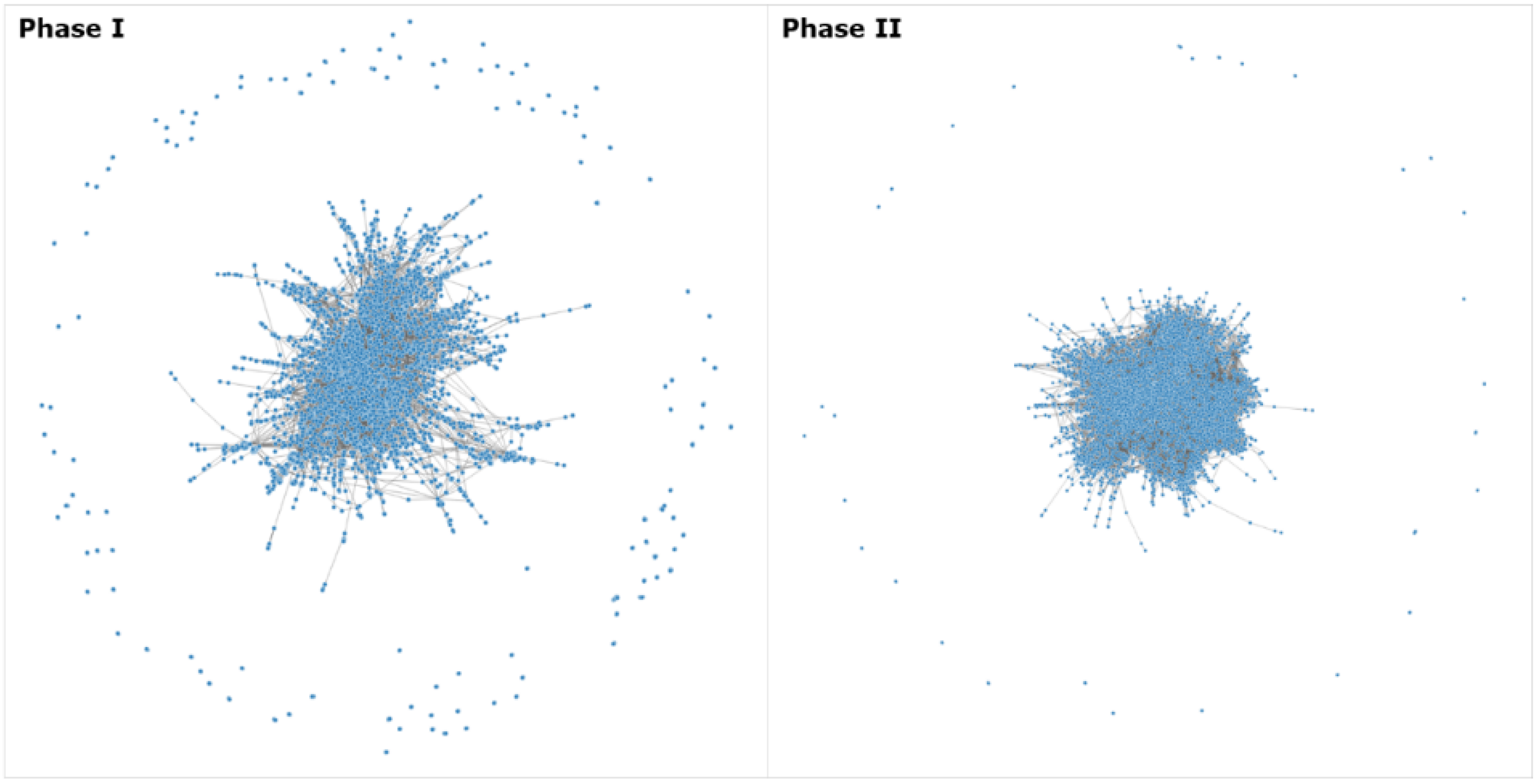
Based on the carbon trading data, we built the network as described in Section 3.1. The results are visualized in Figure 1. The nodes represent the firms which participate in the EU ETS, and the edges are their trading relationships.
For both phases, there is one major network comprising thousands of nodes and edges. Around the major network, there are a few small outlying networks consisting of only a few nodes. As shown in Figure 1, the carbon trading network can be considered a complex network due to its complexities in both network structure and evolution. In this section, we propose an integrated method to analyze the network. First, time windows (as defined in Section 3.4) were introduced to make the network time-varying. Through these time windows, the evolutionary features of the network can be observed, including, for example, the growth of the network nodes and edges. Second, metric indicators (defined in Section 3.2) are used to measure the structural features of the network. The evolution of those features is also analyzed with the time windows. Finally, the scale-free feature of the carbon trading network is tested by both linear regression and segmented linear regression (as mentioned in Section 3.3).
As shown in Table 2, the label of a time window, namely (or ), corresponds to a specific time range. For example, represents the time range of 1 January 2005 to 1 May 2008 of Phase I, and represents the time range of 1 January 2008 to 1 July 2008 of Phase II. For ease of comparison, the labels for the time windows of Phase I and II are combined in all following figures. In the combined labels, the time window of Phase I and of Phase II share the same label because they have 4 months of overlap.
4.1. Growth Features of the Carbon Trading Network
The size of the EU carbon market can be measured by the number of nodes and edges. The overall sizes of the networks are reported in Table 3. In Phase I, 4605 firms built 7803 trading relationships with each other. It may be noted that 106 firms are missing compared to the number of firms listed in Table 1; this is because those firms did not trade any allowances with other firms—in other words, they did not build any trading relationships in the EU ETS. In Phase II, the number of firms grew to 6644, which built 19,393 trading relationships with each other—a striking increase from Phase I.
Figure 2 reports the number of nodes and edges observed during each time window. As is shown, the number of nodes and edges increased significantly during both phases. During the first year of the Phase I market (label ), carbon trading was a new concept for firms, and the first surrender of allowances had not yet been executed, so the number of firms and trading relationships increased very slowly. From then on, as the pressure of allowance surrenders increased, firms gradually entered the trading market and the size of the Phase I market increased continuously. Additionally, as previously mentioned, the Phase I market was a trial market, and it was closed on May 2008. However, it can be observed from Figure 2 that the Phase I market still displayed an increasing tendency at the end of the market.
The Phase II market is the successor of the Phase I market. In Phase II, the market size increased rapidly at the beginning. By the first surrender of Phase II (label ), the Phase II market size was already equivalent to that of the final Phase I market. After , the number of firms plateaued, but the trading relationships continued to increase at a rapid pace.
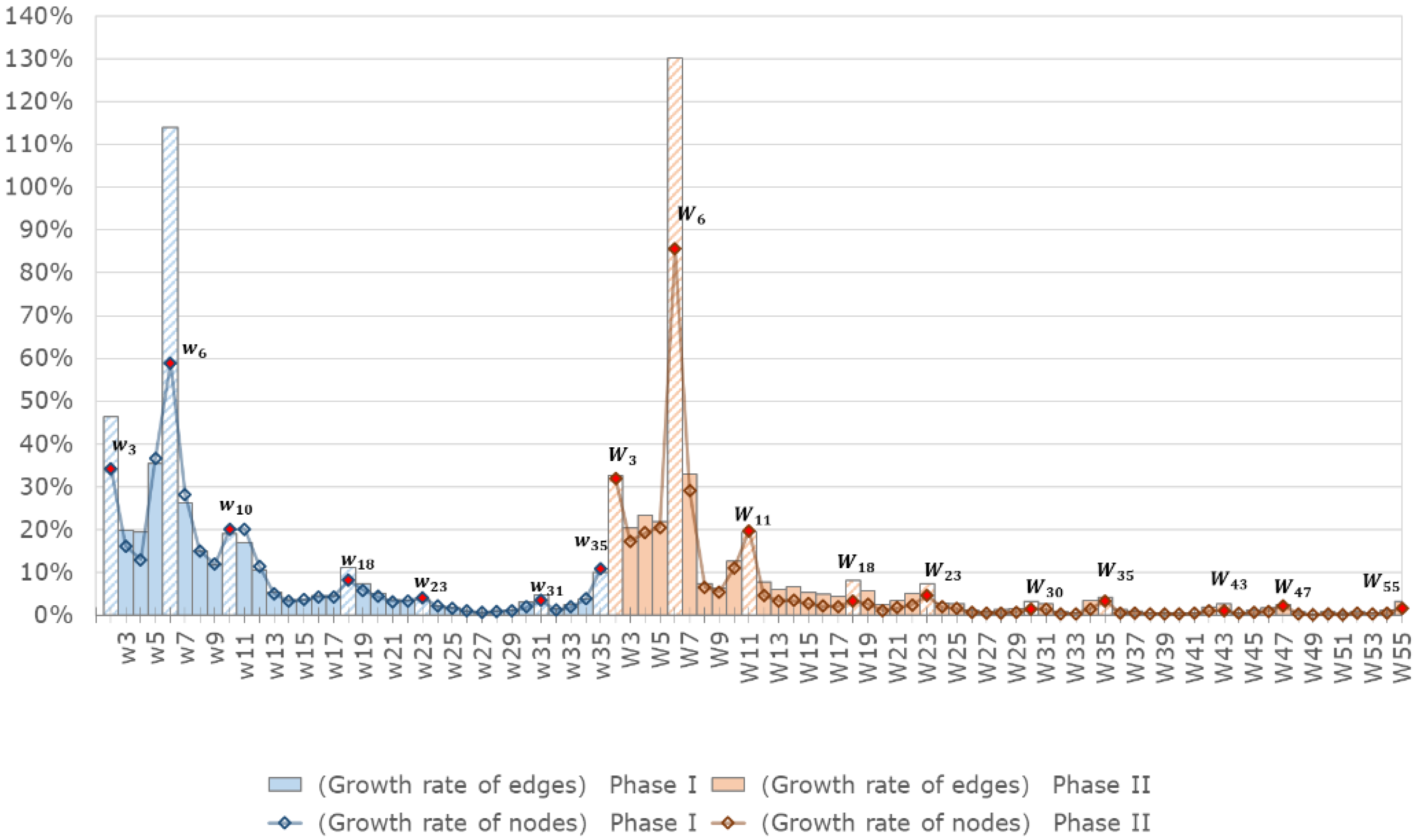
Figure 3 illustrates the growth rate of the nodes and edges, in which the extremum values are marked (red points and textured columns). For both nodes and edges, the extremum value of growth appears in the same periods, namely, , , , , , , and for Phase I, and , ,, , , ,, , and for Phase II.
Generally, the extremum values appear twice in each year: once around May, when firms are required to surrender allowances, and once around December, when most active future contracts expire. These are the periods when there are high levels of activity in carbon trading, and it can be seen that the size of the carbon trading network increased rapidly at those times. However, the growth rates of nodes and edges decreased significantly outside of those periods. The growth rate decreased to 5% after the first surrender (label of Phase I or label of Phase II), and decreased even further to 1% after the second surrender (label of Phase I or label of Phase II). These decreases in growth rates imply that the scale of the markets became increasingly stable. It is also notable that the nodes and edges grew rapidly in the last 2 months of Phase I (label and ), when the Phase I market was about to be closed. Once the Phase I market was closed, the value of the Phase I allowances would disappear; hence, lots of firms swarmed into the market to sell their remaining allowances as fast as they could.
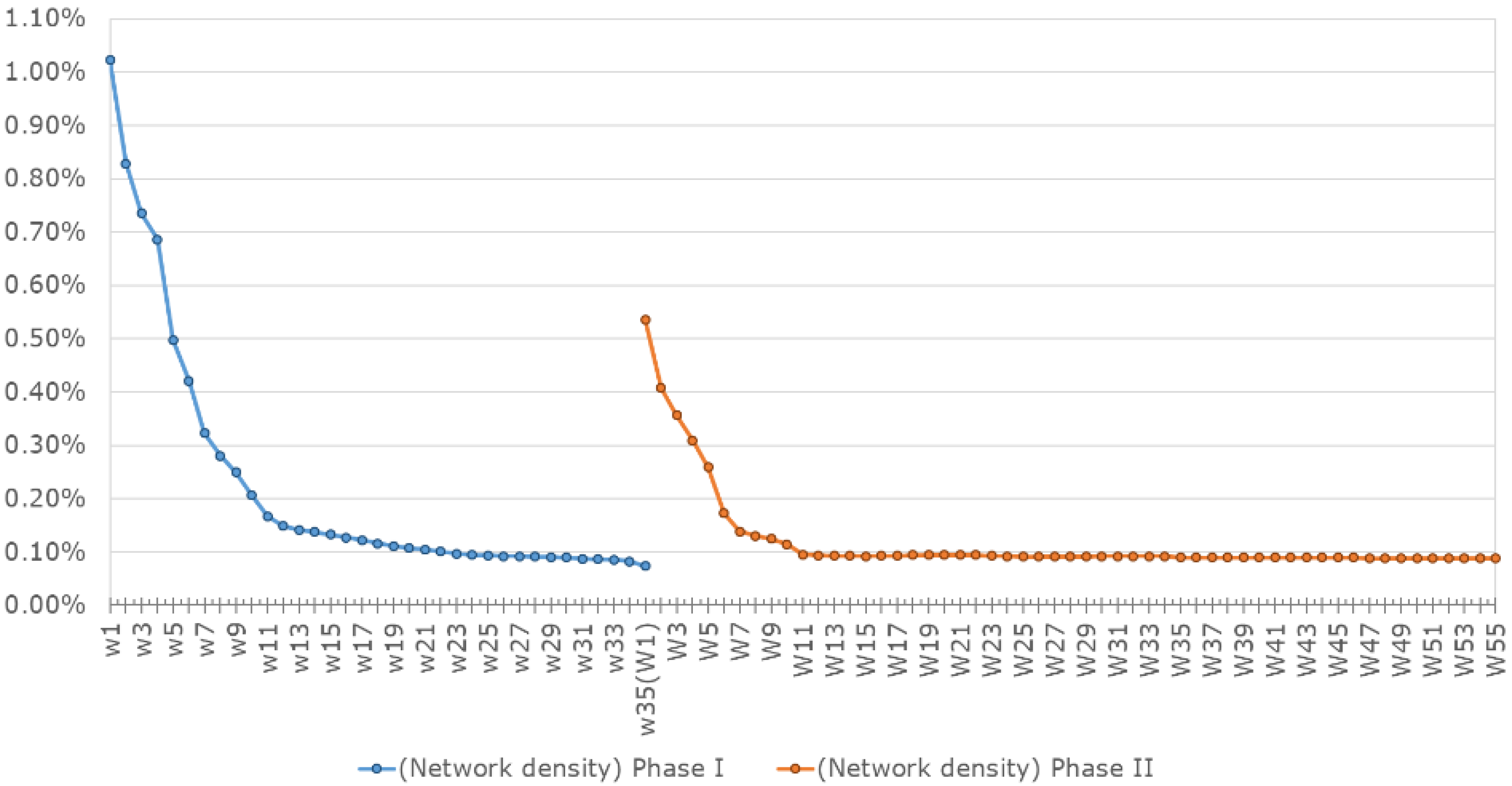
Figure 4 illustrates the network densities of the carbon trading network. As is shown, network density decreased rapidly at the beginning of both phases, but then the decrease became steadier over time. Specifically, network density converged at the level of 0.1% after the second surrender of Phase I (label ), as well as following the first surrender of Phase II (label ), thus proving that the market structures were stabilizing.
It can also be noticed that in both phases, the levels of network density were very low, even when the market structures were stable. For example, in Phase I, there were 4605 firms in the time window . According to Equation (1), these firms represented a potential for more than 21 million relationships. However, only 19,393 relationships were built, representing a very low network density value of 0.074%. It can therefore be concluded that the connection of the network was far from complete.
4.2. Structural Features of the Carbon Trading Network
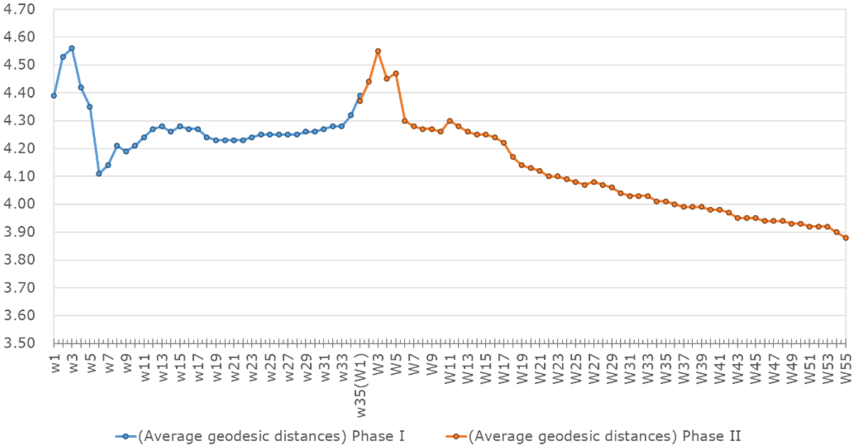
As discussed in Section 3.2, average geodesic distance measures the difficulty of finding trade partners. Therefore, it can be used as an indicator of market efficiency in terms of information and allowance transfers.
Figure 5 illustrates the changes over time in average geodesic distance for the carbon trading networks. In Phase I, the average geodesic distance fluctuated sharply at the beginning of the phase but was then confined to a range of 4.2 to 4.3 after the first allocation, when the market structures became stable, before sharply increasing in the last 2 months when the market was about to close. In Phase II, the average geodesic distance also fluctuated significantly at the beginning of the phase; however, the value then decreased gradually over time from 4.3 to 3.88. From this it can be concluded that the carbon market became increasingly efficient over time in terms of information and allowance transfers, as finding trading partners became increasingly easy for firms. However, this quantitative change did not lead to a qualitative change, because on average each firm needed at least 2 “bridge firms” in order to find an appropriate trading partner.
As previously explained, the clustering coefficient describes market efficiency in terms of competitiveness. Figure 6 shows that the average clustering coefficient gradually increased during both phases, indicating that the firms were inclined to cluster together in carbon trading. As more firms clustered together, the power of firms with a dominant trading position was weakened by the extensiveness of trading relationships. It can therefore be concluded that the competitiveness and efficiency of the market were increasing.
4.3. Scale-Free Features of the Carbon Trading Network
In complex network theory, if the distribution of a network satisfies the power law (see Equation (6)), then the network is said to be a scale-free network. To test whether carbon trading is a scale-free network, we apply both linear and segmented linear modeling to the trading data from both phases. The time windows of and are chosen for modeling the networks because the market is more stable at the end of each period.
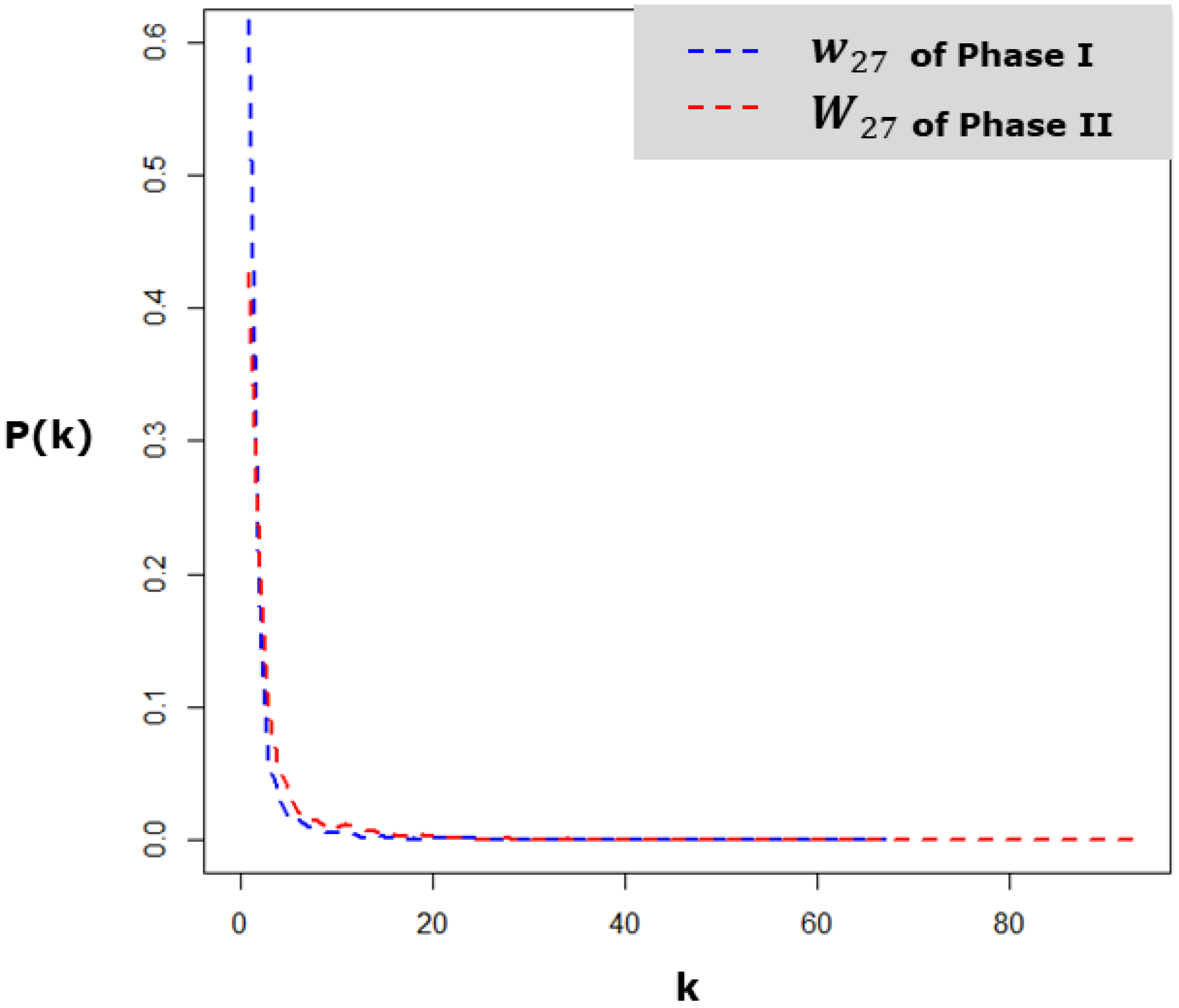
Figure 7 illustrates the degree distribution of both networks. As is shown, the probability density of degree decreases sharply towards zero as degree grows. This reveals that most firms in the EU ETS have only few trading partners, but a few firms have a vast number of trading partners. Notably, the density curve of is steeper than the density curve of . In the time window of , about 61% of firms had only one trading partner, while about 4.5% of firms had more than 10 trading partners. By contrast, in the time window of , only 42% of firms had only one trading partner, but about 10% of firms had more than 10 trading partners.
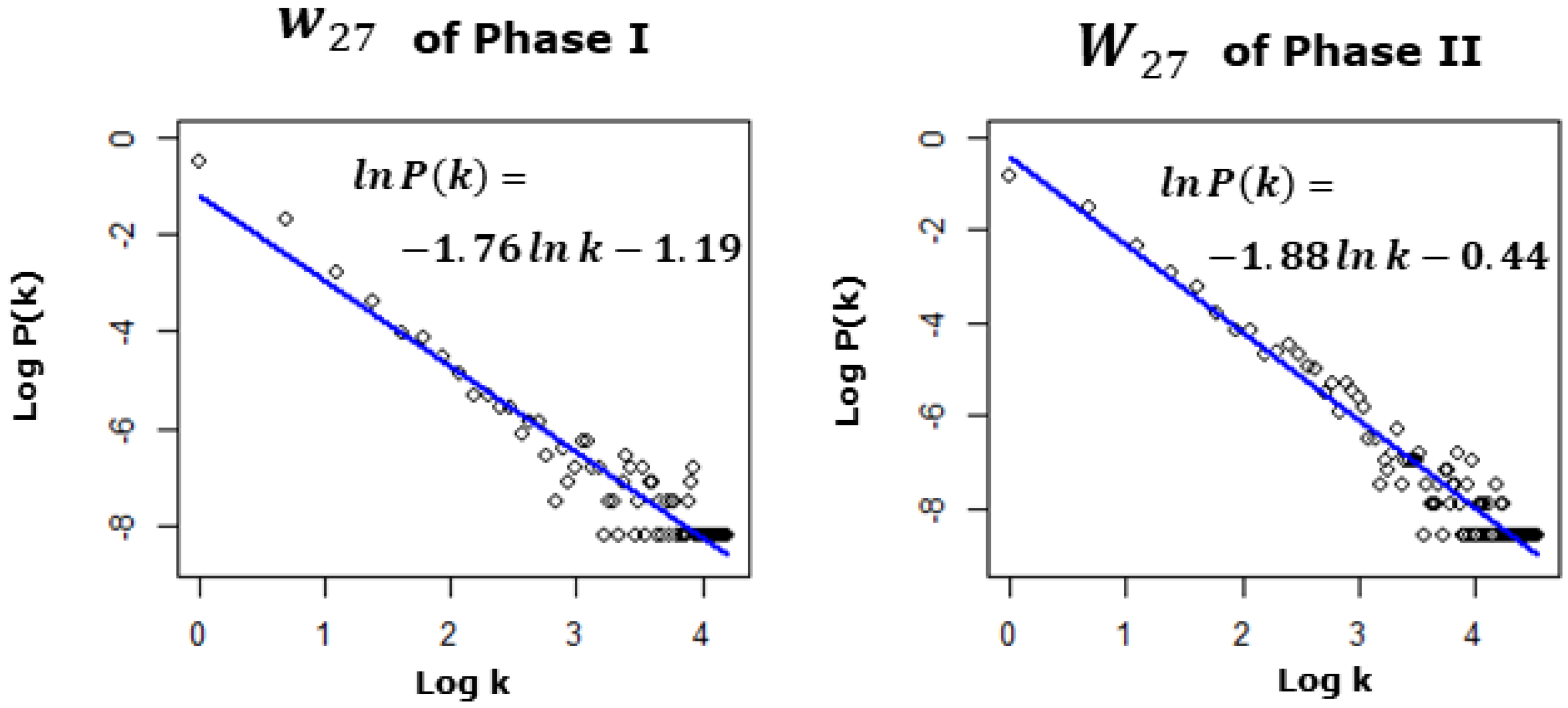
When logarithms are taken of both and , their relationship becomes linear, as shown in Figure 8. As an essential characteristic of power law, the linear relationship between and can be modeled by the following model:
where and respectively indicate the scaling and intercepting exponents. The linear least square method has been commonly used in previous research to estimate the exponents. Therefore, we separately estimate the exponents for the two networks of and . As shown in Table 4, the estimated values of are both significant at a 1% level for both datasets, and the goodness of fit values are both above 90%. However, the residuals analysis shows that the linear model of Equation (10) is invalid (Table 4) for both networks. For the network, the insignificance of Shapiro-Wilk implies that the residuals obey the normal distribution, but the significance of Durbin-Watson implies the residuals exhibit heteroscedasticity. Therefore, the linear model is invalid for . For Phase II, the model is also invalid because the residuals exhibit heteroscedasticity.
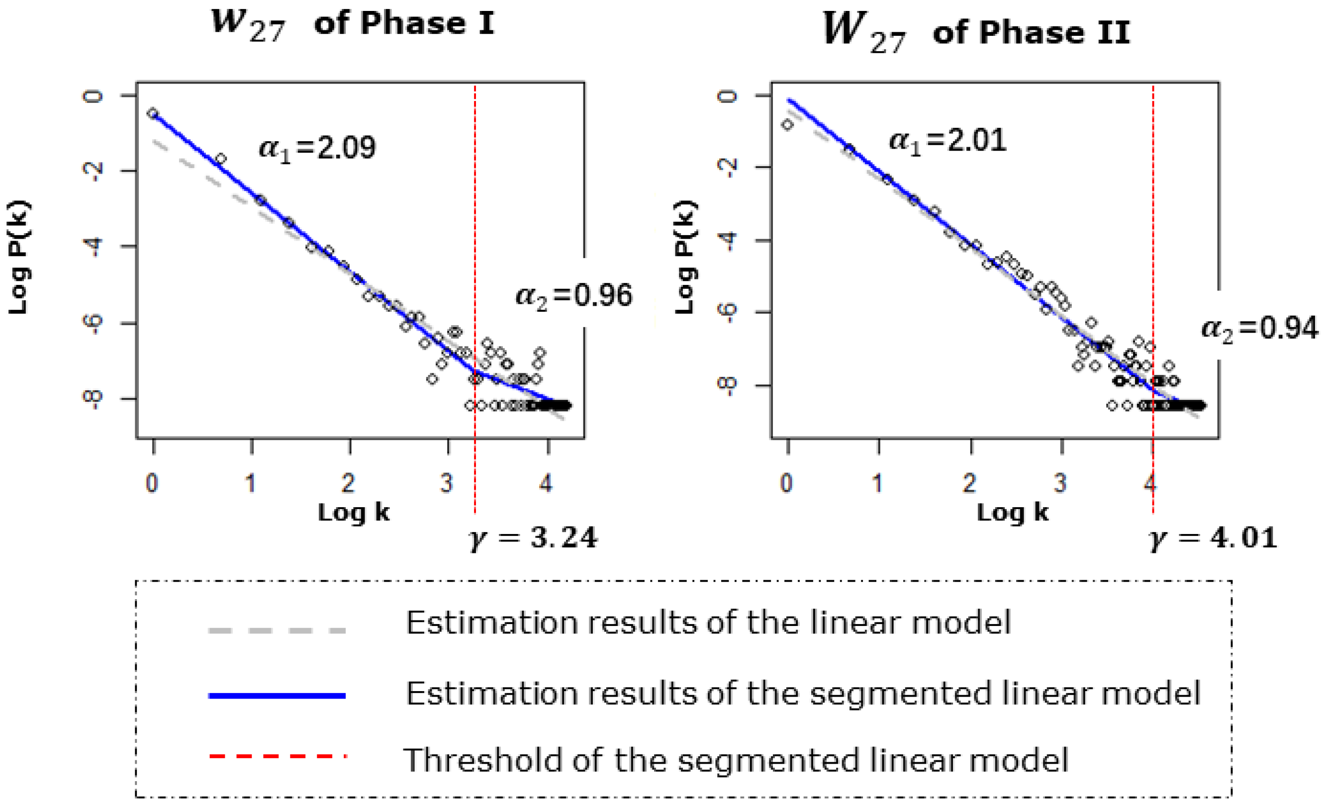
Since the linear model is invalid, we try to model the data using the broken power law. By performing logarithmic transformations on Equations (7) and (8), segmented linear models can be built as follows:
In the segmented linear model, , , and are the exponents which can be estimated by segmented linear regression. is the threshold of the broken power law.
As shown in Table 5, for both networks, all the estimated exponents were significant at a 1% level, and the goodness of fit () values are higher than 90%. The residuals analysis shows that both the Shapiro-Wilk test and the Durbin-Watson test of the residuals are insignificant at a 5% level, which indicates that the broken power law model is valid. As shown in Figure 9, the form of the broken power law was similar for the two networks. Therefore, while we only discuss the results of , the same conclusions can be drawn for the other.
In the network, the estimated value of the exponent is 3.24, so the threshold of the broken power law is about 25. If the nodes degree is less than 25, then the degree distribution obeys a power law of which the exponent is 2.10; otherwise, the degree distribution follows another power law of which the exponent is 1.18. According to Equation (6), the density function of the former power law is steeper than the latter, which brings a higher heterogeneity to the network.
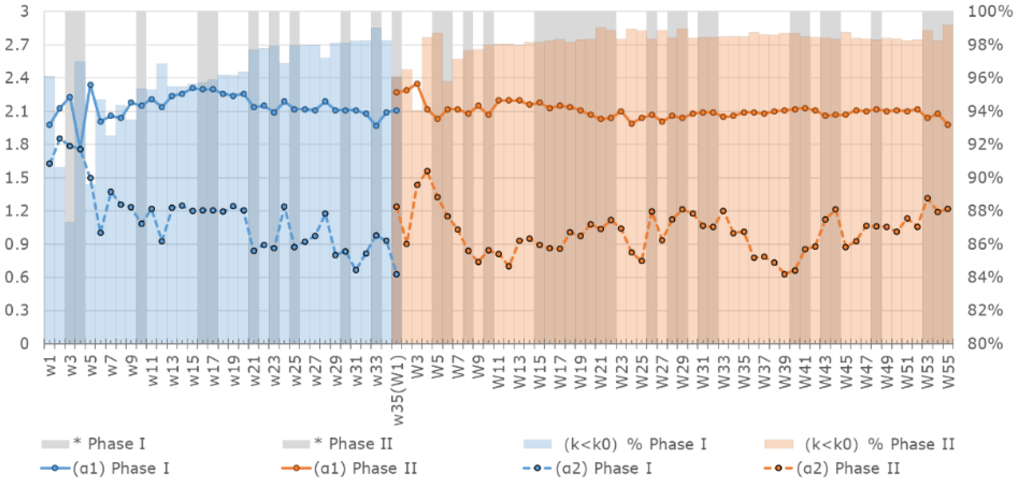
By applying the broken power law model to each time window, we illustrate the changes in the exponents and validity of the broken power law model (Figure 10). First, the broken power law distribution is invalid around the periods when firms and trading relationships increased rapidly (e.g., and for Phase I or and for Phase II). Second, for the firms whose degree was below the threshold, the heterogeneity in trading relationships is higher and stable. Third, for the firms whose degree is above the threshold, the heterogeneity in trading relationships is lower and unstable. Fourth, the degree distribution of the overall carbon trading network can be approximately described as the first part of the broken power law distribution (the power law in Equation (7)), because more than 95% of the firms had trading partners below the threshold of the broken power-law (see the colored columns in Figure 10). Compared to the approximated power law model, the broken power law model is flatter in the lower tail of the distribution, which leads to a long tail effect on the data.
5. Conclusions
Using firm-level carbon trading data from the EU carbon market, this paper has constructed an unweighted network model for carbon trading. As tested in our previous work, the data contains all firms and carbon trades in Phase I and Phase II of the EU ETS. Therefore, this network presents a full picture of the trading relationships in the EU carbon market. By integrating time windows into the network model, we are able to analyze the growth, structural, and scale-free features of the market from an evolutionary perspective. Some meaningful results are concluded as follows:
- (1)
- We analyze the growth features of the carbon trading network for both Phase I and Phase II. Because the EU carbon market is an emerging market, the size of the market became increasingly larger with the development of the market. Over the long term, the growth rate decreased gradually over time, implying that there is a growth for the market. However, in the short run, the growth rate of the market is accelerated in May and December of each year. As the growth rate cooled down, the market structure become stable.
- (2)
- We calculate the average geodesic distances and average clustering coefficients for the network model. Both metric indicators reveal that the market structures are evolving towards efficiency. First, the average geodesic distances are gradually decreasing, showing that over time the firms find it easier to find appropriate trading partners in the carbon trading network. Therefore, the market become more efficient in terms of transferring information and allowances. Second, the average clustering coefficients gradually increase over time, implying that firms are inclined to cluster together. Firms’ clustering behavior will potentially weaken the market power of firms with a dominant position in the trading networks, leading to a more structurally efficient market. Third, although the metric indicators’ trends are ideal, the actual changes were too small to significantly increase market efficiency.
- (3)
- Both a power law model and a broken power law model are built to test whether the carbon trading network is a scale-free network. Through a residuals analysis, the power law model is found to be invalid for the carbon trading network, although the estimation results are significant. By contrast, the significance and validity of the broken power law model prove that the degree distribution of the carbon trading network consisted of two power laws. The steeper degree distribution is suitable for modeling the heterogeneity of firms with fewer trading partners, which apply to more than 95% of all firms. Therefore, the broken power law can be approximately understood as a traditional power law, but the long tail effect should be noted when using the approximate power law model.
- (4)
- Finally, we test the network with the broken power law model in each time window. The results show that, for most of the time, the relationships between firms in the EU carbon market obey a similar broken power law as the one that apply to the overall market. The model only invalid when the market approaches a high growth rate.
Author Contributions
Y.L. carried out the analysis for research question. He wrote most of the manuscript and conducted the data processing. X.G. contributed to the establishment of the network model and he wrote part of the introduction regarding to the modelling. J.G. supervised the work and contributed to the discussions of the results, he also contributed to revising the paper.
Acknowledgments
This work is financially supported by National Natural Science Foundation of China (No. 71671180), Chinese Key Research Plan Project (No. 2016ZX05040-001), Beijing Natural Science Foundation (No. 9174041). We would like to thank the weekly CEEP-CAS Seminar, which acted as fertile ground for this research idea.
Conflicts of Interest
The authors declare no conflict of interest.
References
- Trotignon, R.; Delbosc, A. Allowance Trading Patterns During the EU ETS Trial Period: What Does the CITL Reveal? Eur. Environ. 2008, 13, 1–36. [Google Scholar]
- Zaklan, A. Why Do Emitters Trade Carbon Permits? DIW Discuss. Pap. 2013, 1275, 32. [Google Scholar]
- Ellerman, A.D.; Convery, F.J.; de Perthuis, C. Pricing Carbon: The European Union Emissions Trading Scheme; Cambridge University Press: Cambridge, UK, 2010. [Google Scholar]
- Benz, E.; Trück, S. Modeling the Price Dynamics of CO2 Emission Allowances. Energy Econ. 2009, 31, 4–15. [Google Scholar] [CrossRef]
- Conrad, C.; Rittler, D.; Rotfuß, W. Modeling and Explaining the Dynamics of European Union Allowance Prices at High-Frequency. Energy Econ. 2012, 34, 316–326. [Google Scholar] [CrossRef]
- Koch, N.; Fuss, S.; Grosjean, G.; Edenhofer, O. Causes of the EU ETS price drop: Recession, CDM, renewable policies or a bit of everything? New evidence. Energy Policy 2014, 73, 676–685. [Google Scholar] [CrossRef]
- Chan, H.S.R.; Li, S.; Zhang, F. Firm competitiveness and the European Union emissions trading scheme. Energy Policy 2013, 63, 1056–1064. [Google Scholar] [CrossRef]
- Crossland, J.; Li, B.; Roca, E. Is the European Union Emissions Trading Scheme (EU ETS) informationally efficient? Evidence from momentum-based trading strategies. Appl. Energy 2013, 109, 10–23. [Google Scholar] [CrossRef]
- Martino, V.; Trotignon, R. Back to the Future: A Comprehensive Analysis of Carbon Transactions in Phase 1 of the EU ETS. Available online: https://www.chaireeconomieduclimat.org/en/publications-en/information-debates/id-27-a-comprehensive-analysis-of-carbon-transactions-in-phase-1-of-the-eu-ets/ (accessed on 8 June 2018).
- Balietti, A.C. Trader types and volatility of emission allowance prices. Evidence from EU ETS Phase I. Energy Policy 2016, 98, 607–620. [Google Scholar] [CrossRef]
- Bushnell, J.B.; Chong, H.; Mansur, E.T. Profiting from Regulation: Evidence from the European Carbon Market. Am. Econ. J. Econ. Policy 2013, 5, 78–106. [Google Scholar] [CrossRef]
- Oestreich, A.M.; Tsiakas, I. Carbon Emissions and Stock Returns: Evidence from the EU Emissions Trading Scheme. J. Bank. Financ. 2015, 58, 294–308. [Google Scholar] [CrossRef]
- Mizrach, B.; Otsubo, Y. The market microstructure of the European climate exchange. J. Bank. Financ. 2014, 39, 107–116. [Google Scholar] [CrossRef] [Green Version]
- Newman, M.E.J. The structure and function of complex networks. Siam Rev. 2003, 45, 167–256. [Google Scholar] [CrossRef]
- De Andrade, R.L.; Rêgo, L.C. The use of nodes attributes in social network analysis with an application to an international trade network. Phys. A Stat. Mech. Appl. 2018, 491, 249–270. [Google Scholar] [CrossRef]
- Sun, Q.; Gao, X.; Zhong, W.; Liu, N. The stability of the international oil trade network from short-term and long-term perspectives. Phys. A Stat. Mech. Appl. 2017, 482, 345–356. [Google Scholar] [CrossRef]
- Liang, S.; Feng, Y.; Xu, M. Structure of the Global Virtual Carbon Network: Revealing Important Sectors and Communities for Emission Reduction. J. Ind. Ecol. 2015, 19, 307–320. [Google Scholar] [CrossRef]
- Tian, X.; Geng, Y.; Sarkis, J.; Zhong, S. Trends and features of embodied flows associated with international trade based on bibliometric analysis. Resour. Conserv. Recyc. 2018, 131, 148–157. [Google Scholar] [CrossRef]
- Liu, Y.P.; Guo, J.F.; Fan, Y. A big data study on emitting companies’ performance in the first two phases of the European Union Emission Trading Scheme. J. Clean. Prod. 2017, 142, 1028–1043. [Google Scholar] [CrossRef]
- Fan, Y.; Liu, Y.P.; Guo, J.F. How to explain carbon price using market micro-behaviour? Appl. Econ. 2016, 48, 4992–5007. [Google Scholar] [CrossRef]
- Liu, Y.; Zhao, C.; Wang, X.; Huang, Q.; Zhang, X.; Yi, D. The degree-related clustering coefficient and its application to link prediction. Phys. A Stat. Mech. Appl. 2016, 454, 24–33. [Google Scholar] [CrossRef]
- Bauke, H. Parameter estimation for power-law distributions by maximum likelihood methods. Eur. Phys. J. B 2007, 58, 167–173. [Google Scholar] [CrossRef] [Green Version]
- Virkar, Y.; Clauset, A. Power-law distributions in binned empirical data. Ann. Appl. Stat. 2014, 8, 89–119. [Google Scholar] [CrossRef]
- Jóhannesson, G.; Björnsson, G.; Gudmundsson, E.H. Afterglow Light Curves and Broken Power Laws: A Statistical Study. Astrophys. J. 2006, 640, L5–L8. [Google Scholar] [CrossRef]
- Muggeo, V.M.R. Estimating regression models with unknown break-points. Stat. Med. 2003, 22, 3055–3071. [Google Scholar] [CrossRef] [PubMed]
- Muggeo, V.M.R. Segmented: An R package to fit regression models with broken-line relationships. R News 2008, 8, 20–25. [Google Scholar]
- Watts, D.J. Networks, dynamics, and the small-world phenomenon. Am. J. Sociol. 2016, 105, 493–527. [Google Scholar] [CrossRef]
- Choromański, K.; Matuszak, M.; MiȩKisz, J. Scale-Free Graph with Preferential Attachment and Evolving Internal Vertex Structure. J. Stat. Phys. 2013, 151, 1175–1183. [Google Scholar] [CrossRef] [Green Version]
- Barabási, A.-L.; Albert, R. Emergence of scaling in random networks. Science 1999, 286, 509–512. [Google Scholar] [PubMed]
- Pachon, A.; Sacerdote, L.; Yang, S. Scale-free behavior of networks with the copresence of preferential and uniform attachment rules. Phys. D Nonlinear Phenom. 2018, 371, 1–12. [Google Scholar] [CrossRef] [Green Version]
Figure 1.
Visualization of the carbon trading networks.

Figure 2.
The number of nodes and edges. Note: in the oriental axis, and are the labels for the time windows of Phase I and Phase II, respectively.
Figure 2.
The number of nodes and edges. Note: in the oriental axis, and are the labels for the time windows of Phase I and Phase II, respectively.

Figure 3.
The growth rate of nodes and edges. Note: in the oriental axis, and are the labels for the time windows of Phase I and Phase II, respectively.
Figure 3.
The growth rate of nodes and edges. Note: in the oriental axis, and are the labels for the time windows of Phase I and Phase II, respectively.

Figure 4.
Network density. Note: in the oriental axis, and are the labels for the time windows of Phase I and Phase II, respectively.
Figure 4.
Network density. Note: in the oriental axis, and are the labels for the time windows of Phase I and Phase II, respectively.

Figure 5.
Average geodesic distances. Note: in the oriental axis, and are the labels for the time windows of Phase I and Phase II, respectively.
Figure 5.
Average geodesic distances. Note: in the oriental axis, and are the labels for the time windows of Phase I and Phase II, respectively.

Figure 6.
Average clustering coefficient. Note: in the oriental axis, and are the labels for the time windows of Phase I and Phase II, respectively.
Figure 6.
Average clustering coefficient. Note: in the oriental axis, and are the labels for the time windows of Phase I and Phase II, respectively.

Figure 7.
Degree distribution of networks during and .

Figure 8.
Degree distribution in log–log coordinates and estimation results of the linear model.

Figure 9.
Estimation results of the linear and segmented linear models.

Figure 10.
Evolution of scale-free features. Note: In the horizontal axis, and are labels of the time windows for Phase I and Phase II, respectively; the series “( ) %” is the proportion of firms whose trading partners are below the threshold of the broken power law. The vertical axis on the left is for the exponents of and; the vertical axis on the right is for the series “() %”; the shadow column indicates that the broken power law model was invalid in the period.


Table 1.
Features of the EUTL data.
| Features | Phase I | Phase II |
|---|---|---|
| Account-level data | ||
| OHA | 8214 | 13,408 |
| PHA | 782 | 4285 |
| Total account | 8996 | 17,693 |
| Trades | 48,931 | 311,314 |
| Firm-level data | ||
| Emitter | 4711 | 6349 |
| Financial institution | 15 | 332 |
| Total firms | 4726 | 6681 |
| Trades | 41,490 | 298,177 |
Table 2.
Time window settings.
| Phase I | Phase II | |
|---|---|---|
| Labels | ||
| 1 January 2005 | 1 January 2008 | |
| 1 May 2008 | 1 January 2013 | |
| 6 months | 6 months | |
| 1 month | 1 month | |
| From 1 to 35 | From 1 to 55 |
Table 3.
Overall size of the carbon trading networks.
| Phase I | Phase II | |
|---|---|---|
| Number of nodes— | 4605 | 6644 |
| Number of edges— | 7803 | 19,393 |
| Network density— | 0.074% | 0.088% |
Table 4.
Power law estimations.
| Estimated Results | of Phase I | of Phase II |
|---|---|---|
| 1.76 *** | 1.88 *** | |
| Goodness of fit () | 0.91 | 0.94 |
| Shapiro-Wilk test of the residuals | 0.97 | 0.96 ** |
| p-value of Shapiro-Wilk test | 6.2% | 1.1% |
| Durbin-Watson test of the residuals | 1.35 ** | 1.16 |
| p-value of Durbin-Watson test | 0.2% | 7.0% |
Note: *** and ** indicates the results significant at 0.1% and 1% level respectively.
Table 5.
Broken power-law estimations.
| Estimation Results | of Phase I | of Phase II |
|---|---|---|
| 2.09 *** | 2.01 *** | |
| 0.96 ** | 0.94 ** | |
| 3.24 | 4.01 | |
| 25.53 | 55.14 | |
| Goodness of fit () | 93% | 95% |
| % of nodes of which degree is smaller than | 98.0% | 98.9% |
| Residuals Analysis | ||
| Shapiro-Wilk test of the residuals | 0.98 | 0.98 |
| p-value of Shapiro-Wilk test | 24.8% | 7.3% |
| Durbin-Watson test of the residuals | 1.83 | 1.94 |
| p-value of Durbin-Watson test | 14.0% | 26.5% |
Note: *** and ** indicates the results significant at 0.1% and 1% level respectively.
© 2018 by the authors. Licensee MDPI, Basel, Switzerland. This article is an open access article distributed under the terms and conditions of the Creative Commons Attribution (CC BY) license (http://creativecommons.org/licenses/by/4.0/).
Share and Cite
MDPI and ACS Style
Liu, Y.; Gao, X.; Guo, J. Network Features of the EU Carbon Trade System: An Evolutionary Perspective. Energies 2018, 11, 1501. https://doi.org/10.3390/en11061501
AMA Style
Liu Y, Gao X, Guo J. Network Features of the EU Carbon Trade System: An Evolutionary Perspective. Energies. 2018; 11(6):1501. https://doi.org/10.3390/en11061501
Chicago/Turabian StyleLiu, Yinpeng, Xiangyun Gao, and Jianfeng Guo. 2018. "Network Features of the EU Carbon Trade System: An Evolutionary Perspective" Energies 11, no. 6: 1501. https://doi.org/10.3390/en11061501
Note that from the first issue of 2016, this journal uses article numbers instead of page numbers. See further details here.